the Creative Commons Attribution 4.0 License.
the Creative Commons Attribution 4.0 License.
 | 14 Jun 2022
Quantifying the uncertainty of precipitation forecasting using probabilistic deep learning
Nengcheng Chen
Chao Yang
Hongchu Yu
Zeqiang Chen
Precipitation forecasting is an important mission in weather science. In recent years, data-driven precipitation forecasting techniques could complement numerical prediction, such as precipitation nowcasting, monthly precipitation projection and extreme precipitation event identification. In data-driven precipitation forecasting, the predictive uncertainty arises mainly from data and model uncertainties. Current deep learning forecasting methods could model the parametric uncertainty by random sampling from the parameters. However, the data uncertainty is usually ignored in the forecasting process and the derivation of predictive uncertainty is incomplete. In this study, the input data uncertainty, target data uncertainty and model uncertainty are jointly modeled in a deep learning precipitation forecasting framework to estimate the predictive uncertainty. Specifically, the data uncertainty is estimated a priori and the input uncertainty is propagated forward through model weights according to the law of error propagation. The model uncertainty is considered by sampling from the parameters and is coupled with input and target data uncertainties in the objective function during the training process. Finally, the predictive uncertainty is produced by propagating the input uncertainty in the testing process. The experimental results indicate that the proposed joint uncertainty modeling framework for precipitation forecasting exhibits better forecasting accuracy (improving RMSE by 1 %–2 % and R2 by 1 %–7 % on average) relative to several existing methods, and could reduce the predictive uncertainty by ∼28 % relative to the approach of Loquercio et al. (2020). The incorporation of data uncertainty in the objective function changes the distributions of model weights of the forecasting model and the proposed method can slightly smooth the model weights, leading to the reduction of predictive uncertainty relative to the method of Loquercio et al. (2020). The predictive accuracy is improved in the proposed method by incorporating the target data uncertainty and reducing the forecasting error of extreme precipitation. The developed joint uncertainty modeling method can be regarded as a general uncertainty modeling approach to estimate predictive uncertainty from data and model in forecasting applications.
- Article
(3380 KB) - Full-text XML
- BibTeX
- EndNote


Precipitation is a key hydrometeorological variable in earth system science and is the main driving factor of floods and droughts (Xu et al., 2019). In 2019 the flood disaster driven by extreme precipitation caused a direct economic loss of USD 29.6 billion in China, and the drought disaster led to a crop production loss of 2.36×10¹⁰ kg (http://www.mwr.gov.cn/sj/#tjgb, last access: 6 April 2022). Accurate precipitation forecasting is vital for the early warning of flood and drought, smart city management and agricultural water resources allocation (Van Den Hurk et al., 2012; Pozzi et al., 2013). However, the precipitation forecasting problem suffers from uncertainties from data, algorithms and random factors (Reeves et al., 2014; Kobold and Sušelj, 2005; Xu et al., 2020b). The predictive uncertainty is a measurement of the spread of precipitation forecasting and could indicate how much the forecasted precipitation values fluctuate around the mean (Papacharalampous et al., 2020). Therefore, the uncertainty range should be given when generating precipitation forecasting results.
The precipitation forecasting methods can be divided into two categories: numerical weather forecasting and statistical machine learning. Numerical models consider the physical process of earth system and could simulate the interactions between atmospheres, oceans and lands (Sikder and Hossain, 2016; Molinari and Dudek, 1992). Numerical models have strong physical meaning and are the dominant ways of operational precipitation forecasting. However, the forecasting ability of numerical models is limited due to the uncertainty in initial and boundary conditions, the imperfection of parameterization schemes, and the uncertainty in parameters (Reeves et al., 2014; Xu et al., 2021a). With the development of computer technology and machine learning algorithms, using random data-driven techniques for precipitation forecasting has become popular in recent years (Shi et al., 2015; Trebing et al., 2021; Sønderby et al., 2020). The accuracy of data-driven methods is comparable to currently advanced numerical models in short-term (e.g., from hours to weeks) precipitation forecasting. For example, the convolutional long-short term memory (LSTM) network is shown to outperform the physical optical flow method in precipitation nowcasting based on radar images (Shi et al., 2015). Another deep learning model called MetNet showed advantages over traditional numerical models in terms of the forecasting accuracy and running time for hourly precipitation prediction (Sønderby et al., 2020). The data-driven methods also exhibit appealing results in subseasonal to seasonal precipitation forecasting relative to numerical models (Boukabara et al., 2019; Chantry et al., 2021; Hwang et al., 2019). A key drawback of data-driven precipitation forecasting methods is the lack of physical meaning, also known as black-box model. Despite this feature, data-driven statistical machine learning methods have been widely used for parameter calibration, data processing, submodel replacement and process understanding among physical simulations (Ardabili et al., 2019; Sahoo et al., 2017; Reichstein et al., 2019). The data-driven learning techniques are strong complements to numerical models for the improvement of precipitation forecasting accuracy.
The predictive uncertainty in precipitation forecasting arises mainly from data and models (Gal, 2016). The data uncertainty comes from external observation conditions, instruments and processing algorithms. The data uncertainty is usually examined by perturbing initial conditions in numerical models and producing a perturbed multi-model ensemble, which is widely seen in hydrometeorological ensemble forecasting (Xu et al., 2019; Gneiting and Raftery, 2005; Duan et al., 2019; Vitart et al., 2017). The data uncertainty is rarely investigated in data-driven precipitation forecasting and is often assumed to be accurate without error. The model uncertainty is often represented by an ensemble of perturbed model physics and parameters in numerical weather forecasting (Vitart et al., 2017; Kirtman et al., 2014; Taylor et al., 2012). In data-driven models, the model uncertainty is generally modeled by random regularization of parameters (Gal, 2016; Kendall and Gal, 2017). For linear regression, the parametric uncertainty is indicated by the standard deviation of trained parameters. In deep learning, the network layers could be randomly abandoned to prevent overfitting and generate a forecasted ensemble by Monte Carlo sampling (Kendall and Gal, 2017; Srivastava et al., 2014; Loquercio et al., 2020; Ghahramani, 2015).
The data and model uncertainties should be considered jointly in an integrated modeling framework to get the predictive uncertainty, as the data and model uncertainties could both inflate the predictive spread considerably (Gal, 2016; Kendall and Gal, 2017). It is expected that the forecasting result would be more or less different if the used data and parameters are randomly sampled from the population. Data uncertainty is usually assumed as a constant or Gaussian distribution and could be propagated into final forecasting through error forward propagation (Loquercio et al., 2020; Xu et al., 2020a). If the data uncertainty is unknown, it can be learned from the training process by considering the data uncertainty as a trainable parameter (Kendall and Gal, 2017). However, the joint learning of data errors and model weights will increase the number of training parameters and may mix the error flow from data and parameters. A prior estimation of data uncertainty could help unravel the data error and facilitate the training process. On the other hand, previous forecasting studies usually model the input data uncertainty and ignore the uncertainty in the target (predictand) data (Kendall and Gal, 2017; Loquercio et al., 2020). The uncertainty in the target dataset also plays an important role in the parameter training process and could influence the forecasting accuracy.
There are two ways to estimate the data uncertainty. One is to use in situ ground stations to calculate the systematic and random errors within the data and the other is to use multisource datasets to compute random error by intercomparison (Xu et al., 2021b; Gruber et al., 2016; Sun et al., 2018). The in situ validation method is limited to the number and density of ground stations and is suitable for small areas with enough station coverage. The second method is independent of the in situ stations and requires multisource datasets with independent error distribution (Gruber et al., 2016). There are numerous precipitation datasets from various sensors and models and these could be used to calculate precipitation data error at a large spatial scale (Xu et al., 2020b; Sun et al., 2018). Three-cornered hat (TCH) and triple collocation (TC) are two commonly used methods to evaluate the random error among multisource datasets, which do not require ground measurements as references (Premoli and Tavella, 1993; Mccoll et al., 2014; Stoffelen, 1998). The basic assumption of the TCH and TC methods is the stationarity of both the raw dataset and its error, which may not always be satisfied for real-world data. Most of the existing studies assume that the used multisource datasets obey the stationarity condition when using the TCH or TC methods (Xu et al., 2020b; Gruber et al., 2016, 2017), which is useful for the determination of relative prior random error.
In this study, we aim to quantify the predictive uncertainty of data-driven precipitation forecasting by fully considering the uncertainty from data and models. The data uncertainty is estimated by the TCH method a priori and is assumed as Gaussian distribution. The data uncertainty is propagated within model training by the law of error propagation. The parametric uncertainty is modeled by randomly abandoning some network layers during the training process. The data and model uncertainties are jointly considered in the objective function within a deep learning encoder–decoder framework. The forecasting experiments are conducted to see whether the accuracy of precipitation forecasting can be improved by joint data–model uncertainty modeling relative to several uncertainty processing strategies from the existing studies.
The study area is located in southern and northern China, East Asia (Fig. 1). The annual rainfall decreases from the southeast to the northwest, with an approximate average rainfall of 1500 mm in the southeast regions and 300 mm in the northwest areas. Most of the southern areas feature a subtropical monsoon climate and the rainfall is relatively larger in summer and smaller in winter. From June to July in 2020, extreme precipitation hit southern China (Wei et al., 2020) and caused a direct economic loss of USD 13.2 billion. The precipitation forecasting in the southern area of China is very challenging and meaningful. Previous studies use numerical models for precipitation forecasting in this area and show some values (Yuan et al., 2012; Luo et al., 2017). The northern area of China features the temperate moon and continental climates, with an annual rainfall of 400–800 mm in the main rainy season of July and August. Here we would like to explore the possibility of weekly precipitation forecasting by a data-driven deep learning method.
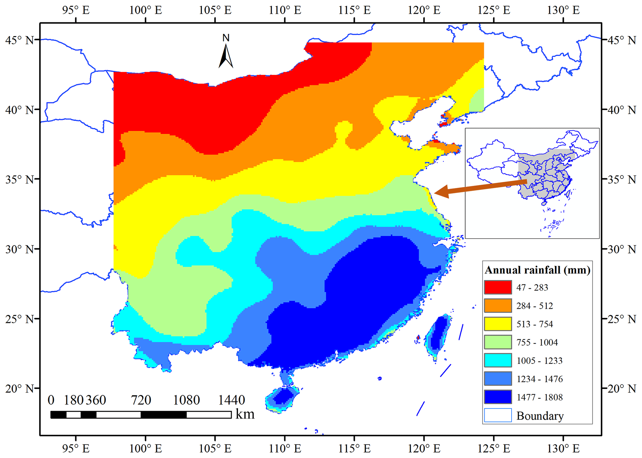
Figure 1The study area for short-term precipitation forecasting.
Multisource precipitation datasets are used to obtain the data error and to measure the precipitation forecasting ability of different uncertainty processing strategies, including datasets from 1980 to 2020 of the Modern-Era Retrospective Analysis for Research and Applications, version 2 (MERRA-2) (Gelaro et al., 2017), the National Centers for Environmental Prediction Reanalysis version 2 (NCEP R2) (Saha et al., 2014) and the European Centre for Medium-Range Weather Forecasts Reanalysis version 5 (ERA-5) (Hersbach et al., 2020). The datasets with 2 m surface temperature and geopotential height at 500 hPa are collected from the three datasets accordingly as predictors. All these daily datasets are converted to weekly data and are bilinearly interpolated into 0.25∘ resolution. In the forecasting process, the temperature and geopotential height predictors in the historical three consecutive weeks are used to forecast the precipitation in the target week. For example, the predictors in the first week (P1), second week (P2) and third week (P3) are used to forecast the total precipitation in the fourth week.
3.1 Estimation of data uncertainty
The TCH method (Xu et al., 2020b; Premoli and Tavella, 1993) is used to estimate the uncertainty in temperature, geopotential height and precipitation datasets. The collected three datasets are all reanalysis data, which are generated from different physical models and data assimilation algorithms. The different reanalysis datasets and their errors are generally not closely correlated and are regarded as collocated datasets for the uncertainty estimation, similar to existing studies (Xu et al., 2021b; Mccoll et al., 2014; Gruber et al., 2017). In the TCH algorithm, one arbitrary dataset is chosen as the reference among the three datasets, and then the differencing operation is conducted between the reference and the other two datasets to get the differencing series. The covariance of the differencing series is connected to the variance–covariance matrix of precipitation datasets through matrix transformation. The parameters of the variance–covariance matrix are iteratively resolved by minimizing the global correlation of the covariance of the differencing series. A detailed introduction of the TCH method could refer to Premoli and Tavella (1993) and Xu et al. (2020b).
Consider the data series . It can be generally expressed as
where Ptrue denotes the true predictor or predictand data in a specific area and is unknown, and εi is the measurement error. Choosing an arbitrary dataset as the reference, the differences of N−1 data and the reference data are calculated as
where PN is the reference series and the TCH result is independent of the selection of reference data. These N−1 differences are concatenated into an matrix
where the rows of D denote the differenced time series with M length. The variance/covariance of D is then obtained by
where represents the average of D. The covariance of D can be related to S by
where R is the N×N covariance matrix of and u represents the vector [1 ⋯1]T. The covariance matrix of D is regarded as the Allan covariance when TCH was initially proposed to evaluate the instability of clocks, which requires a filtering operation on the original time series before differencing. However, the covariance can also be the commonly mentioned sample variance. Equation (5) can be reformatted as
where is the matrix and r is the (N−1) vector grouping covariance estimates with the Nth time series and rNN denotes the variance of the Nth time series. This partitioning can help solve the underdetermined problem in Eq. (5) by isolating the N free parameters (r and rNN). When the free parameters are determined, the unknown elements in are obtained by
A suitable objective function is suggested by Galindo and Palacio (1999) based on the Kuhn–Tucker theorem to minimize the quadratic mean of covariances
subjected to a constraint
where . The initial conditions are selected as follows to meet the constraint (Torcaso et al., 1998):
Once the free parameters are determined, the unknown elements in R can be solved using Eq. (7).
The uncertainties of the predictors and predictands are estimated weekly using the TCH method. The weekly datasets are grouped according to the weekly climatology and then used to estimate the uncertainty. For example, all the precipitation datasets which belong to the first week of each year are concatenated to apply the TCH method in order to get the uncertainty of the datasets for the first week of each year. Similarly, the data uncertainty for the 2nd and 3rd week until the 52nd week is evaluated sequentially. This strategy enables a time-variant uncertainty estimation which is more reasonable as the precipitation climatology is different for different seasons. The NCEP R2 and ERA-5 data are used to assist the uncertainty estimation of MERRA-2 data by the TCH method, and the precipitation forecasting experiments are conducted based on MERRA-2 data to evaluate the proposed forecasting framework.
3.2 Variational Bayesian inference
Here we introduce the variational inference theory (Hoffman et al., 2013), which is a standard Bayesian modeling technique for the estimation of model uncertainty. Given the input data and the output data , the Bayesian regression is used to find suitable parameters within the function y=fw(x) which could generate the output Y according to the input X. The parameter w is assumed to obey a prior distribution p(w) before the observations are known. When the observed data are obtained, it is possible to determine which parameters are more suitable for the function according to the data. A likelihood distribution is defined to describe the probability of y generated by x and w. For example, a Gaussian likelihood function is defined as
where τ−1 is the observation noise and I is the identity matrix.
Given the input data X and the output data Y, the Bayesian theorem is applied to find the posterior distribution of parameters in the parameter space
where the numerator p(Y|X) is the normalization factor, also named as model evidence
The solution of Eq. (13) needs to marginalize the likelihood over w, which is analytically tractable for some simple models such as the Bayesian regression, but intractable for complex models such as deep learning methods (Gal, 2016).
Given the new input data x′, the forecasted value is generated by the integral of probability over the parameter space, which is called the inference process:
Since the posterior distribution of parameters cannot be obtained analytically, an approximate analytical distribution qθ(w) could be defined, with θ as the parameter to be estimated, being as close as the posterior distribution. The Kullback–Leibler (K–L) divergence (Kullback and Leibler, 1951) is an indicator to measure the similarity of two distributions, also known as relative entropy. The objective function is to minimize the K–L divergence between the two distributions:
The optimal variational distribution qθ′(w) is obtained when the K–L divergence is minimized. The estimated variational distribution could be regarded as the posterior distribution of parameters and then the predictive distribution could be generated:
The above inference process is the variational Bayesian inference. Variational inference replaces the integral of the likelihood with optimization, which simplifies the estimation of posterior distribution.
3.3 Monte Carlo sampling
The Monte Carlo method is a kind of stochastic simulation technology, proposed by Stanislaw Ulam and John von Neumann during the Second World War (Von Neumann and Ulam, 1951). Monte Carlo methods are used to estimate unknown parameters by random sampling and are widely applied in mathematics, physics, game theory and finance (Brooks, 1998; Jacoboni and Lugli, 2012; Metropolis and Ulam, 1949; Rubinstein and Kroese, 2016).
In Eq. (14), the posterior distribution cannot be solved analytically. Assume Ui as the weight matrix from i−1 layer to i layer, i.e., , a variational weight distribution q(w) is defined to randomly replace the columns with zero (dropout process):
where pi and Hi are variational parameters; zi,j is a binary variable, with a value of zero representing the abandoning of the jth unit in i−1 layer and a value of one the keeping, based on the Bernoulli distribution at the probability pi.
The predictive distribution is estimated after minimizing the K–L divergence:
The predictive mean and variance can be obtained after repeating the dropout process multiple times.
where ut, i is the forecasted value for the ith pixel and the tth ensemble. The calculation of predictive variance is based on the standard deviation of the ensemble which represents the spread of the forecasted values.
The above Monte Carlo sampling and dropout process is the Monte Carlo dropout technique which is used to obtain the model uncertainty here.
3.4 Joint data and model uncertainties modeling
Dropout is a Bayesian method to model the model uncertainty in forecasting (Srivastava et al., 2014). However, the data uncertainty also needs to be considered. Kendall and Gal (2017) regarded the data uncertainty as a trainable parameter and jointly considered data and model uncertainties. However, the predictand data uncertainty is ignored and the learning of data uncertainty increases the number of training parameters. Here we propose an integrated modeling framework to fully incorporate the data and model uncertainties during the training process (Fig. 2). First, the data uncertainties of predictors and predictands are estimated by the TCH method and are assumed as Gaussian distribution:
The sampling methods are used to obtain samples from the data distribution to produce ensemble forecasts. The sampling process is conducted for both predictor data and predictand data. The data uncertainty is randomly sampled T times to generate an ensemble of predictors and predictands. In the meantime, the parameters are randomly dropped out for T times to construct a parametric ensemble. The perturbed data and parameter values are jointly used to calculate the training loss. Obtained from the likelihood of a Gaussian process (Srivastava et al., 2014), the objective function is expressed as follows (Kendall and Gal, 2017):
where N is the sample size; p is the dropout probability; ; θ is the parameter to be estimated; σx and σy are the data uncertainty for predictor and predictand, respectively. The propagated data uncertainty for the lth network layer is represented by . The negative log-likelihood function can be deduced according to the objective function:
where σ is the regression noise, with the mean of zero in a Gaussian distribution.
The objective function consists of a mean square error (MSE) term adjusted by data uncertainty and a regularization term, which is the negative logarithm of the Gaussian likelihood function. The objective function includes an uncertainty parameter σ2, which is determined by the sum of propagated uncertainty and target data uncertainty. The minimization of the negative log-likelihood function could be reached by differentiating the optimization function and setting to zero:
where the minimum value of the negative log-likelihood function could be reached when the data variance equals the square of the difference between the forecasted value and the observation.
Once the network weights are determined according to the objective function, the new input data uncertainty is propagated and the weights are randomly sampled to produce the forecasted ensemble. The predictive mean and variance are calculated from the predictive ensembles:
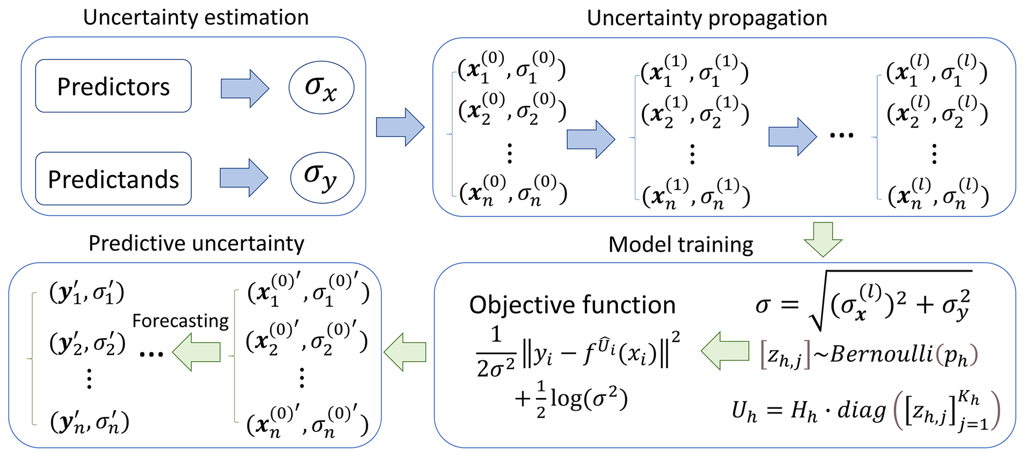
Figure 2The proposed integrated data–model uncertainty modeling framework in precipitation forecasting. σx and σy are the predictor and predictand uncertainty, respectively. and represent the propagated data value and uncertainty, respectively, for the lth network layer.
3.5 The deep learning forecasting framework
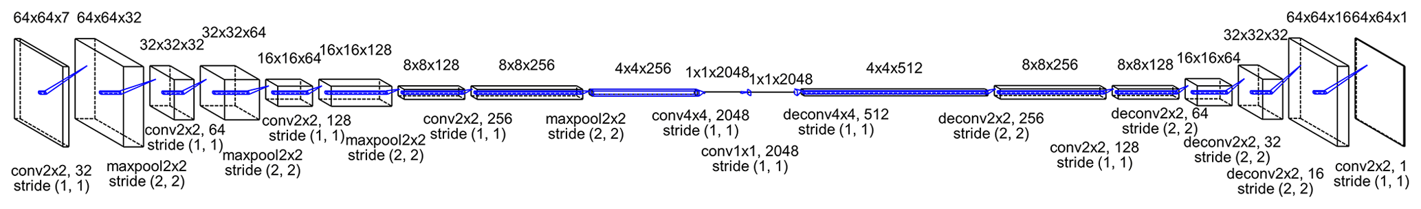
In deep learning, encoder–decoder is a commonly used forecasting model (Badrinarayanan et al., 2017; Cho et al., 2014). In the encoder process, an input signal is converted into a one-dimensional vector with fixed length. In the decoder process, the one-dimensional vector is transformed into the target data with variable length. The available networks used for encoder and decoder processes are arbitrary and depend on the specific problem, such as the convolutional neural network (CNN), recurrent neural network (RNN) and LSTM network (Hochreiter and Schmidhuber, 1997; Goodfellow et al., 2016). The CNN network is used in this study to construct the encoder–decoder forecasting model. Here we designed a deep learning encoder–decoder model for weekly precipitation forecasting (Fig. 3). The temperature and geopotential height data for the previous three weeks are regarded as inputs, with an image size of (including the land–sea mask). In the encoder process, the input image is down-sampled by a series of convolution, pooling and dropout operations, resulting in a one-dimensional vector (). In the decoder process, the one-dimensional vector is up-sampled by deconvolution, dropout and convolution operations, resulting in a forecasted precipitation image (). The down-sampling and up-sampling procedures are used to learn the nonlinear mapping relationships between predictors and predictands.
In the training process, the optimization algorithm is set to Adam (Kingma and Ba, 2014), which is a stochastic learning algorithm based on adaptive moment. The network learning rate is set to 0.001 and the stopping rule of iteration is that the validating error does not decrease for at least 100 times. The data uncertainty is propagated forward according to the law of uncertainty propagation and the dropout process is repeated 10 times with a dropout rate of 0.5. The random seed is set to 1 to enable the reproducibility of the experiment. The experimental data span from 1980 to 2020 (2139 weeks), of which 60 %, 20 % and 20 % of the data are used for training, validating and testing, respectively. The optimal model parameters are determined based on the minimal validating loss.
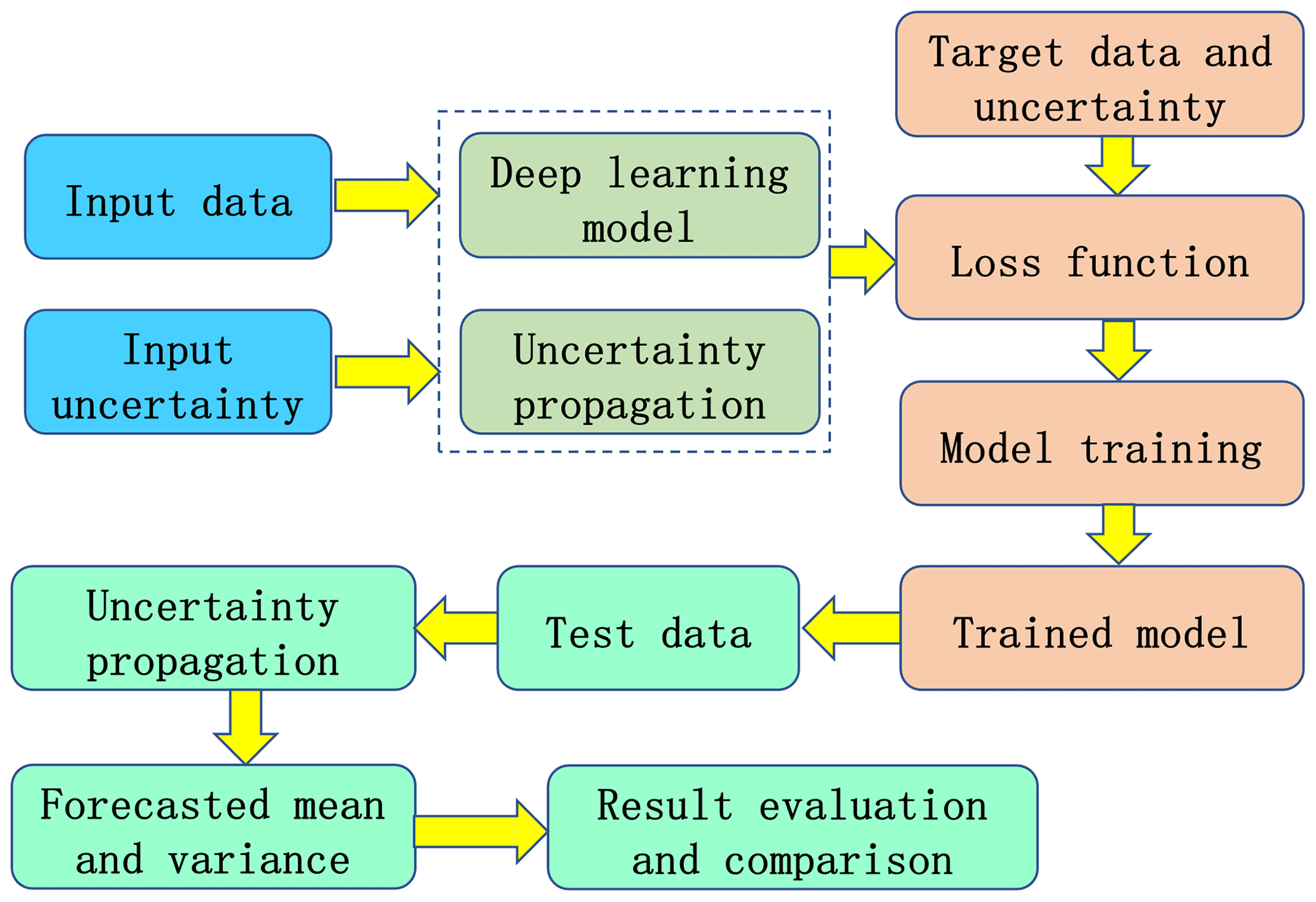
The proposed deep learning framework for precipitation forecasting is demonstrated in Fig. 4. The input data and its uncertainty are prepared and are considered as inputs for the forecasting model. The model weights are initialized and the input uncertainty is propagated forward according to the weights. The loss function value is calculated according to the forecasted value, the propagated uncertainty, target data and its uncertainty. The forecasting model is trained according to the optimization algorithm and then the trained model is obtained. Next the test data are used to produce the forecasted value and variance based on the model weights and uncertainty propagation. Finally, the forecasted value and variance are evaluated and compared with several precipitation forecasting methods.
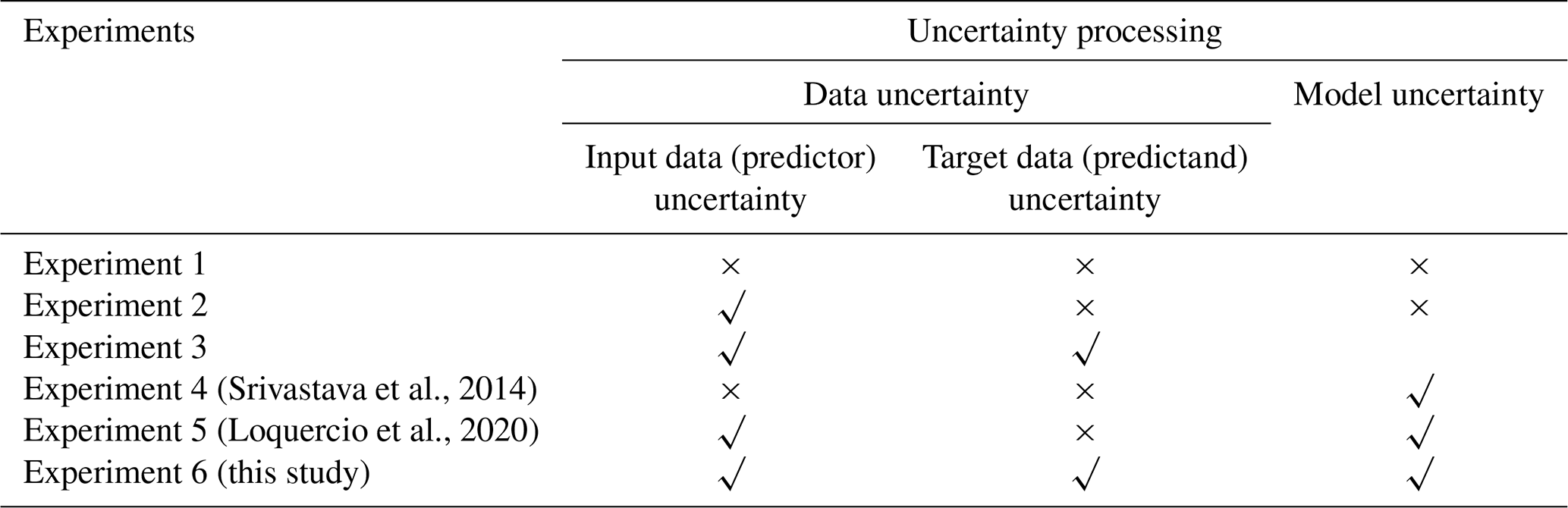
We designed a series of comparison experiments to investigate the effect of different uncertainty processing strategies on the forecasting performance (Table 1). The precipitation forecasting experiment without considering uncertainty is used as the baseline (Experiment 1). The MSE is used as the loss function, and the data and model uncertainties are not considered in Experiment 1. The uncertainty sources are incorporated differently into the experiments, including predictor uncertainty (Experiment 2), predictor and predictand uncertainties (Experiment 3), model uncertainty (Experiment 4) based on the method of Srivastava et al. (2014), data and model uncertainties (Experiment 5) based on the method of Loquercio et al. (2020) and data and model uncertainties (Experiment 6) based on the proposed framework here. The data uncertainty only includes the propagated uncertainty from the input data in Eq. (26) in Experiment 2, while the propagated uncertainty from the input data and the target data uncertainty are both included in Experiment 3. In Experiment 4, the data uncertainty is ignored and the model parameters are randomly sampled 10 times to get the model spread. In Experiment 5, the input data uncertainty is propagated and the model uncertainty is modeled by sampling the parameters. In Experiment 6, the input uncertainty is propagated and the target data uncertainty is included in Eq. (26) and the model uncertainty is represented by a multiple sampling process.
Table 1A summary of the experiment setup in this study. The √ and × symbols indicate that the specific factor is considered and omitted, respectively.
The root mean square error (RMSE) statistic is used to measure the difference between forecasted value and true value:
where yi is the true value or observation, is the forecasted value and n is the sample size.
4.1 The uncertainty of input and output datasets
The data uncertainty of predictors and predictand is calculated based on the TCH method and shown in Fig. 5. The precipitation data uncertainty is much higher than the temperature and geopotential height variables, with a median of ∼43 % relative uncertainty fraction for precipitation, ∼2 % for temperature and ∼1 % for geopotential height in the MERRA-2 data. This pattern is also seen in the ERA-5 and NCEP R2 datasets. Therefore, the precipitation data suffer from greater uncertainty relative to the input data and the predictand uncertainty should not be ignored in the training process. The combination of the propagated input uncertainty and the predictand uncertainty is used as the adjusted parameter to regularize the loss function, which is relatively reasonable as the data with larger uncertainty should contribute less to the total training loss. It should be noted that the predictor and predictand data are normalized to [0, 1] before uncertainty estimation to ensure a fair comparison of uncertainty value. The high uncertainty for precipitation data is related to strong spatiotemporal heterogeneity of precipitation and the high inconsistency among the reanalysis data (Xu et al., 2020b), while temperature and geopotential height data are much more homogeneous in space and time.
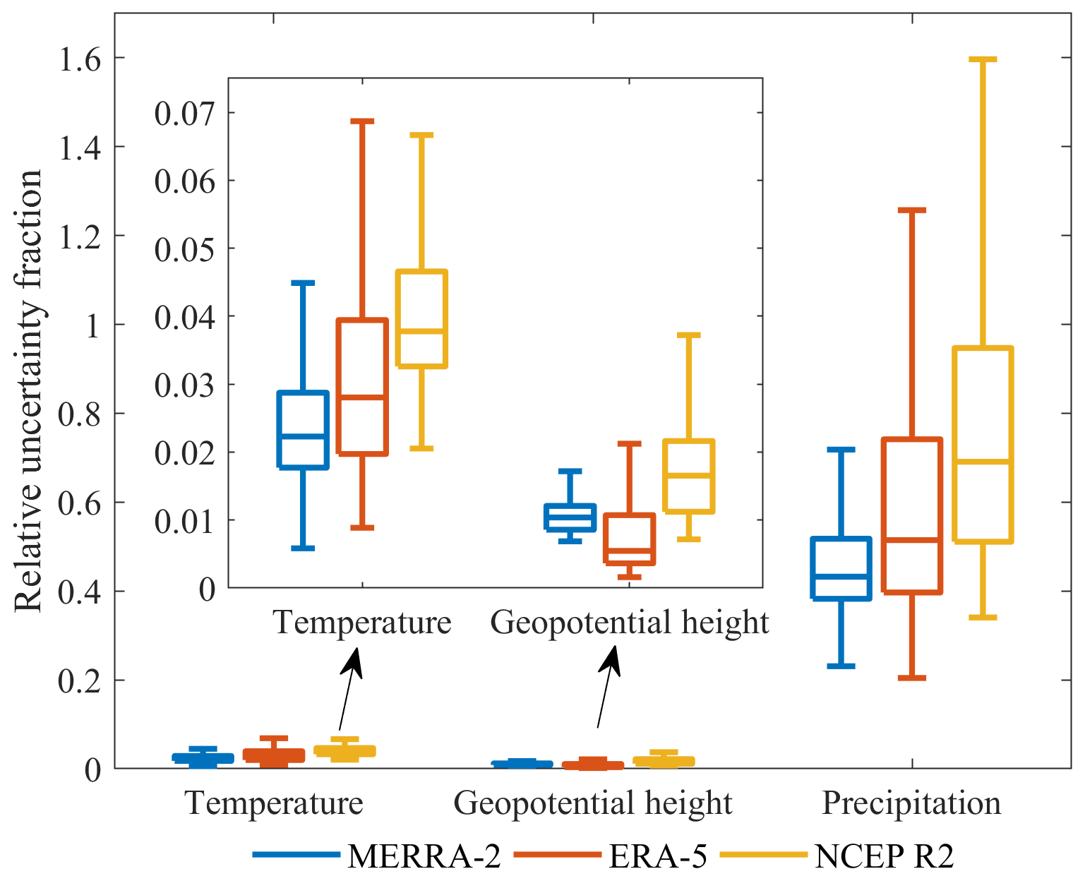
Figure 5The data uncertainty calculated by the TCH method. The uncertainty distribution is plotted according to the uncertainty over all the pixels of the study area.
4.2 Overall precipitation forecasting performance
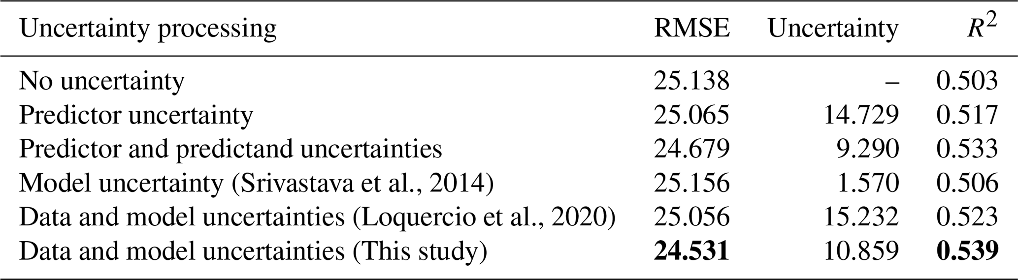
The RMSE and uncertainty in Table 2 are calculated based on the averaged values of all the grid cells. As for the predictive uncertainty, the forecasting method that only considers model uncertainty (Srivastava et al., 2014) obtains the minimum predictive uncertainty (Table 2). However, the data uncertainty is not considered when only sampling from the parameters and thus the impact of data error on forecasting is not evaluated. Loquercio et al. (2020) used the law of uncertainty propagation to propagate the data uncertainty and sampled the parameters randomly during training. In our proposed method, the input data uncertainty, target data uncertainty and model uncertainty are jointly coupled by uncertainty propagation and random parameter sampling. The average predictive uncertainty (10.859) based on the proposed method is smaller than that (15.232) based on the method of Loquercio et al. (2020), and the predictive R2 is higher (0.539) than the latter (0.523). In this regard, the proposed method could reduce the predictive uncertainty of precipitation forecasting to some extent, when jointly modeling data and model uncertainties. The proposed method could improve the precipitation forecasting performance and could improve the reliability of precipitation forecasting by reducing the uncertainty.
When only the input uncertainty is modeled in the forecasting model, the predictive uncertainty is 14.729. If the target data uncertainty is coupled with input uncertainty, the predictive uncertainty is reduced substantially (9.290). In Eq. (30), when the predictive error on the right side of the equation reaches a local minimum and remains unchanged basically, the left side of the equation includes the input uncertainty propagation and the target data uncertainty. When new data are used to make a prediction, the predictive uncertainty is generated by the input uncertainty and the law of error propagation. Thus, when only the input uncertainty is modeled in Eq. (30), the left side of this equation equals the propagated uncertainty from the input data. If the left side of Eq. (30) is replaced from the propagated input uncertainty with the combination of propagated input uncertainty and target uncertainty, the propagated input uncertainty after replacement will be smaller than that of no replacement, i.e., .
The predictive accuracy generally increases with the uncertainty processing procedures. The predictive RMSE decreases when incorporating the predictor uncertainty processing relative to the prediction without uncertainty handling. Further improvement is expected when considering the predictor and predictand uncertainties from the data aspect, relative to the sole predictor treatment. The R2 exhibits slight improvement when incorporating model uncertainty (Srivastava et al., 2014) relative to the prediction without uncertainty processing. In the method of Loquercio et al. (2020), the input data uncertainty and model uncertainty are both considered and the predictive performance increases relative to the no uncertainty and predictor uncertainty processing. In our method, the input data uncertainty, target data uncertainty and model uncertainty are jointly considered, reaching the lowest RMSE and the highest R2 relative to the above uncertainty processing methods.
Table 2The accuracy of precipitation forecasting based on different uncertainty processing strategies. The best RMSE and the highest R2 are shown in bold for each column.
4.3 Spatial patterns of precipitation forecasting
In Fig. 6, the spatial patterns of RMSE for precipitation forecasting demonstrate some similarities and differences between different uncertainty processing strategies. Overall, the spatial distribution of RMSE is similar and smaller in the northwest region but larger in the southeast region. In places where the annual rainfall is abundant, the water cycle process is accelerated and the precipitation observations may suffer from large uncertainty. The difficulty of forecasting extreme high precipitation volume also increases the average RMSE in the southeast region relative to the northwest region (Yuan et al., 2012; Huang et al., 2013). There are some differences in the forecasting error among different forecasting methods in local areas. For example, the forecasting performance based on our proposed method could outperform the methods in Experiments 1, 2, 4 and 5, and is comparable with the method in Experiment 3 for the local areas covered by black circles in Fig. 6.
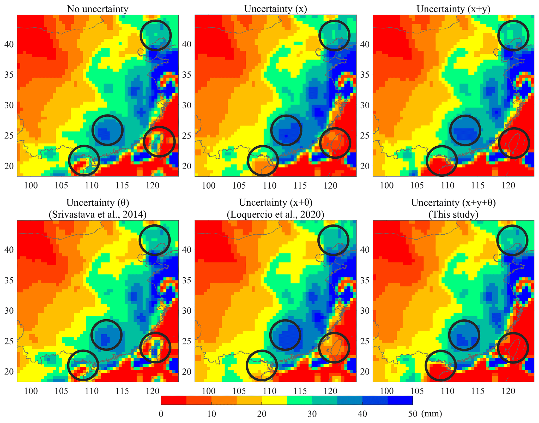
Figure 6The spatial patterns of RMSE for precipitation forecasting. In this figure, x means the modeling of input uncertainty; x+y represents the modeling of input and output uncertainty; indicates the modeling of input uncertainty, output uncertainty and model uncertainty. The black circles represent the highlighted areas.
Figure 7 demonstrates the difference of the predictive RMSE between other uncertainty processing approaches and the proposed method for precipitation forecasting. It can be seen that there is little difference of the predictive RMSE between the proposed method and other uncertainty processing approaches. However, RMSE is larger for some uncertainty processing methods relative to the proposed method in some areas, including the Hainan and Taiwan provinces and part of eastern China. It is likely that the predictive RMSE is reduced in the proposed method by improving the prediction performance in the areas with accelerated water cycle and abundant rainfall. The target data uncertainty is incorporated into the objective function to pay different attentions to space during the training process, leading to a different weight distribution of the forecasting model for the proposed method relative to others. The changing weight distribution improves the forecasting accuracy in the southeast areas by reducing the forecasting error of extreme precipitation.
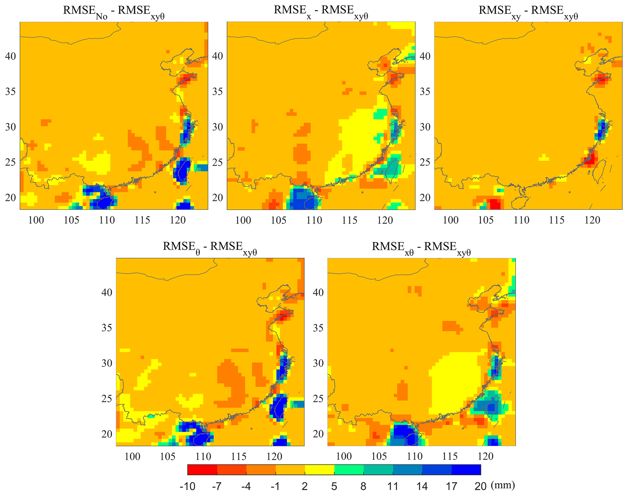
Figure 7The difference of the predictive RMSE between the proposed method and other uncertainty processing approaches for precipitation forecasting.
Figure 8 demonstrates the impact of different uncertainty processing methods on the predictive uncertainty of precipitation. The spatial patterns of predictive uncertainty indicate larger uncertainty in southern China relative to northern China, which is consistent with the knowledge that the water cycle in southern China is accelerated and precipitation forecasting may suffer from large uncertainty. If only the input uncertainty is considered in the forecasting model, the predictive uncertainty is large in the central and southeast regions. The predictive uncertainty could be substantially reduced when incorporating the target data uncertainty besides the input uncertainty. In the method of Loquercio et al. (2020), the predictive uncertainty is slightly higher than that of input uncertainty modeling in space, because the input and model uncertainties are jointly modeled. Our proposed method could include the input, target and model uncertainties jointly and could help reduce the predictive uncertainty to a large extent, relative to the method of Loquercio et al. (2020).

Figure 8The spatial patterns of uncertainty for precipitation forecasting.
4.4 Uncertainty analysis and discussion
In precipitation forecasting, data and model uncertainties both bring uncertainty to the forecasting result. The higher the data and model uncertainties, the more divergent and less reliable the forecasting. Therefore, the data and model uncertainties should be jointly considered in the forecasting process (Gal, 2016; Kendall and Gal, 2017; Loquercio et al., 2020; Parrish et al., 2012). Although the predictive errors are close to each other among different forecasting methods in Fig. 6 and Table 2, the predictive uncertainty has some discrepancies. The modeling of input uncertainty only in the forecasting model would bring high predictive uncertainty and the target data uncertainty is ignored. The joint modeling of input and target uncertainties could reduce the predictive uncertainty substantially, which is related to the change of the variance in Eqs. (26) and (30), corresponding to the minimum value of the forecasting error term. The propagation of input uncertainty is constrained by refining the uncertainty representation in Eq. (26) after incorporating the target uncertainty term and thus changing the weight training process.
Figure 9 demonstrates the relationship between the predictive uncertainty by the proposed method and the summation of the predictive uncertainty from data and model. The predictive uncertainty by the proposed method (σxyθ) agrees well with the summation of the predictive uncertainty from data and model, with a regressed slope of 1.004 and a R2 of 0.98, indicating the good consistency of the predictive uncertainty between joint and separate uncertainty modeling. The median predictive uncertainty is 8.04, 1.40 and 9.49 mm for data, model and joint data–model uncertainty modeling, respectively, in the precipitation forecasting experiments (Fig. 10). The data and model uncertainty account for ∼85 % and ∼15 % of the total predictive uncertainty by the proposed method, respectively. The model structure is fixed in this study and thus the model uncertainty comes from mainly the parameters. The dropout method enables the random abandoning of network parameters over the specific layer and prevents the overfitting of the forecasting model. The distributions of model weights are changed when incorporating the data uncertainty into the objective function (Fig. 11). The model weights become larger and more dispersive relative to the prediction without uncertainty processing or with model uncertainty consideration. The data uncertainty is propagated into the prediction through model weights and thus the data uncertainty contributes more to the predictive uncertainty than model uncertainty. Although the model weights appear more scattered, the predictive accuracy exhibits small improvement due to the uncertainty consideration in the objective function.
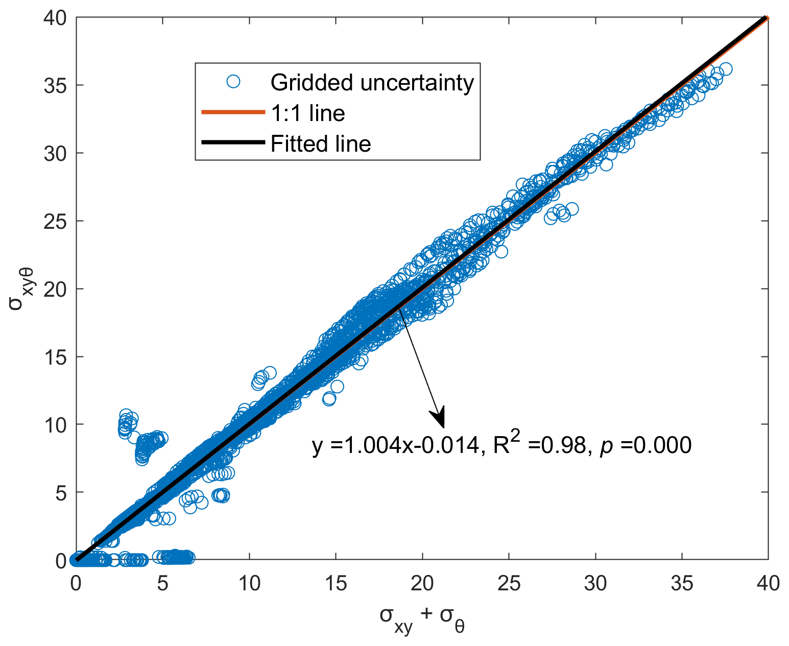
Figure 9The relationship between the summation of predictive uncertainty from data (input and target data) and model and the predictive uncertainty from joint consideration of data (input and target data) and model.
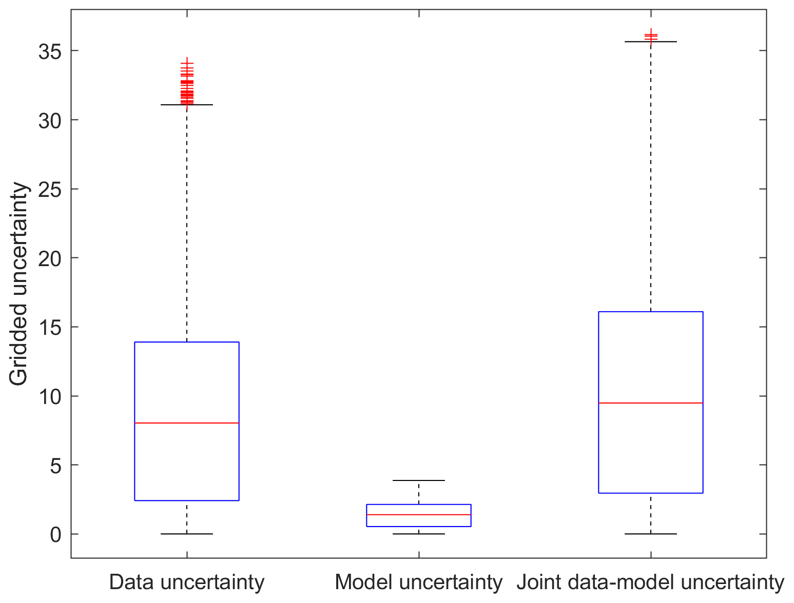
Figure 10The distributions of the predictive uncertainty from data, model and joint data–model modeling methods for precipitation forecasting.
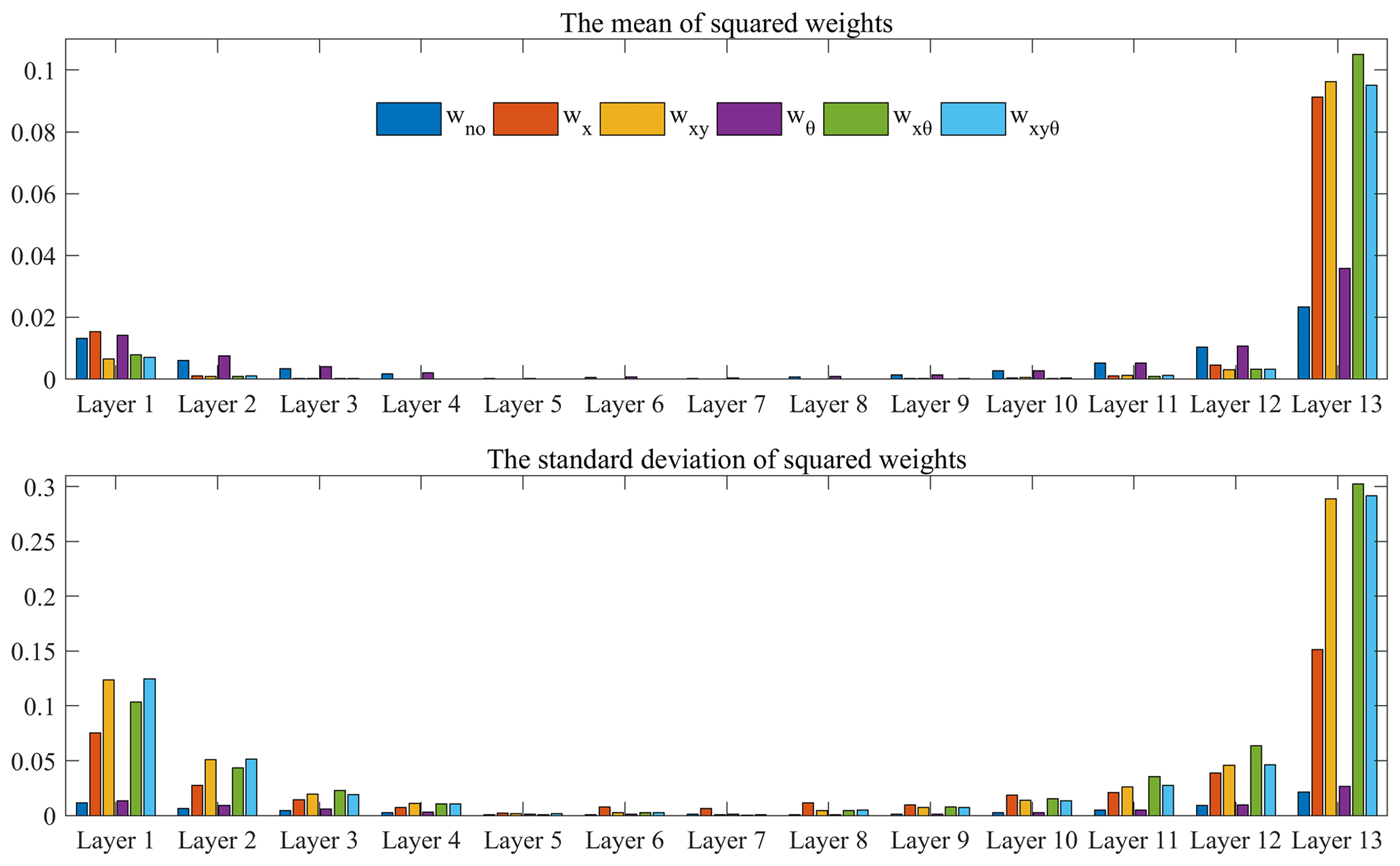
Figure 11The mean and standard deviation of squared weights of the precipitation forecasting model.
The predictive uncertainty is closely related to the input data uncertainty and model weights. In Fig. 2, the input data uncertainty is propagated into predictive uncertainty through model parameters, while the target data uncertainty is incorporated into the training process by the objective function. The incorporation of uncertainty processing changes the training process and the distributions of model weights (Fig. 11). The weights of the last CNN layer (Layer 13) of the precipitation forecasting model are generally higher than the other layers, which may contribute largely to the predictive uncertainty by propagating the data uncertainty. The mean and standard deviation of the squared weights of the last CNN layer for the method of Loquercio et al. (2020) are higher than other uncertainty processing methods, suggesting an overall larger and more dispersive weight distribution for this method than the others. This could partly explain the high uncertainty of the method of Loquercio et al. (2020) in Table 2.
The proposed method in this study could model the input uncertainty, target uncertainty and model uncertainty jointly and could reduce the predictive uncertainty relative to the method of Loquercio et al. (2020). The developed method does not increase the training parameter and is a general forecasting uncertainty method for geophysical applications such as temperature forecasting, runoff forecasting and wind speed forecasting, especially for data-driven forecasting models (Ham et al., 2019; Zheng et al., 2020; Hossain et al., 2015).
In numerical precipitation forecasting systems, ensemble forecasting is commonly used to quantify the predictive uncertainty (Duan et al., 2019). In ensemble forecasting, the model parameters and data are perturbed to produce a forecasted ensemble and thus the data and model uncertainties are both considered. However, it would be time-consuming and cost-expensive to conduct large-sample sampling for complex physical models. In our developed method, the law of error propagation is used to propagate the data uncertainty. The uncertainty propagation of convolution, max-pooling and deconvolution in the deep learning forecasting model is tractable in an analytical form. However, the uncertainty propagation process is generally analytically intractable for complex statistical or physical models. Therefore, the theory and implementation technology for uncertainty modeling require further development, such as surrogate modeling, Monte Carlo methods, polynomial chaos expansions and Bayesian approaches (Linde et al., 2017; Sudret et al., 2017; Zhu and Zabaras, 2018; Schiavazzi et al., 2017; Nitzler et al., 2020).
In this study, we proposed a data–model uncertainty coupling framework to estimate the predictive uncertainty of precipitation forecasting. In this framework, the predictor and predictand uncertainties are estimated a priori by the TCH method and are assumed as Gaussian distribution. The predictor uncertainty is propagated forward during training and testing processes by the law of error propagation. The model uncertainty is represented by randomly abandoning model weights from deep learning layers. The data and model uncertainties are jointly modeled in the objective function during training and are also used during the testing process. The loss function is constructed by the MSE statistic adjusted by data uncertainty and a regularization term based on logarithmic data uncertainty. In the loss function, the adjusting parameter is determined by the combination of the square of predictor and predictand uncertainties. The forecasted ensembles are used to calculate the predictive mean and variance to estimate the predictive uncertainty of precipitation.
The weekly precipitation forecasting in southern and northern China is used as an example to examine the effectiveness of the proposed joint uncertainty modeling framework. Temperature and geopotential height data in the previous three weeks are used to forecast the precipitation in the target week. The forecasting model is developed based on an encoder–decoder CNN deep neural network, with multivariate spatiotemporal predictor data as input and spatiotemporal precipitation data as output. The experimental results indicate that the proposed joint uncertainty modeling framework for precipitation forecasting exhibits better forecasting accuracy (improving RMSE by 1 %–2 % and R2 by 1 %–7 % on average) relative to several existing methods, and could reduce the predictive uncertainty by ∼28 % relative to the approach of Loquercio et al. (2020). The reduction of predictive uncertainty is significative for quantitative precipitation forecasting from a data-driven view. The predictive performance is improved in the proposed method by incorporating the target data uncertainty and reducing the forecasting error of extreme precipitation.
The data-driven precipitation forecasting method has limitations in the interpretation part relative to numerical weather prediction. The precipitation forecasting accuracy for numerical models could still be improved by improving the parameterization schemes and resolving the uncertainties in observations, parameters and models. The proposed uncertainty modeling framework may also provide some insights for the uncertainty quantification in numerical prediction models. For example, the uncertainty propagation for the input data and the coupling with target data uncertainty could be used in a data assimilation scheme to estimate the propagated uncertainty in weather forecasting.
Data-driven precipitation forecasting could be used as a tool to assist regional prediction and warning of extreme weather events together with numerical models. The proposed joint data–model uncertainty modeling framework could help to estimate the forecasting spread and is a general approach to derive predictive uncertainty for geophysical forecasting applications. Further research should focus on the non-Gaussian uncertainty modeling for complex integrated statistical–physical models.
The meteorological data are publicly available and can be obtained via the website https://gmao.gsfc.nasa.gov/reanalysis/MERRA-2/ (GMAO, 2015). for MERRA-2, https://psl.noaa.gov/data/gridded/data.ncep.reanalysis2.html (NOAA, 2022) for NCEP R2 and https://climate.copernicus.eu/climate-reanalysis (ECMWF, 2022). The code is available upon request from the authors.
LX conceptualized and wrote the paper. CY provided supervision of this study. NC gave support in developing the manuscript. HY and ZC reviewed and revised the manuscript.
The contact author has declared that neither they nor their co-authors have any competing interests.
Publisher's note: Copernicus Publications remains neutral with regard to jurisdictional claims in published maps and institutional affiliations.
This research has been supported by the National Key Research and Development Program for Young Scientists (grant no. 2021YFF0704400), the National Key R & D Program (grant no. 2018YFB2100500), the National Natural Science Foundation of China program (grant no. 41890822), the National Natural Science Foundation of China (grant no. 42101429), the Fundamental Research Funds for the Central Universities, China University of Geosciences (Wuhan) (grant no. 162301212687), the Open Fund of State Laboratory of Information Engineering in Surveying, Mapping and Remote Sensing, Wuhan University (grant no. 21S04) and the Fund of Sanya Science and Education Innovation Park of Wuhan University of Technology (grant no. 2021KF0026).
This paper was edited by Yue-Ping Xu and reviewed by two anonymous referees.
Ardabili, S., Mosavi, A., Dehghani, M., and Várkonyi-Kóczy, A. R.: Deep learning and machine learning in hydrological processes climate change and earth systems a systematic review, in: International Conference on Global Research and Education, 52–62, https://doi.org/10.1007/978-3-030-36841-8_5, 2019.
Badrinarayanan, V., Kendall, A., and Cipolla, R.: SegNet: A Deep Convolutional Encoder-Decoder Architecture for Image Segmentation, IEEE T. Pattern Anal., 39, 2481–2495, https://doi.org/10.1109/TPAMI.2016.2644615, 2017.
Boukabara, S.-A., Krasnopolsky, V., Stewart, J. Q., Maddy, E. S., Shahroudi, N., and Hoffman, R. N.: Leveraging modern artificial intelligence for remote sensing and NWP: Benefits and challenges, B. Am. Meteorol. Soc., 100, ES473–ES491, 2019.
Brooks, S.: Markov chain Monte Carlo method and its application, J. Roy. Stat. Soc. D-Sta., 47, 69–100, 1998.
Chantry, M., Christensen, H., Dueben, P., and Palmer, T.: Opportunities and challenges for machine learning in weather and climate modelling: hard, medium and soft AI, Philos. T. Roy. Soc. A, 379, 20200083, https://doi.org/10.1098/rsta.2020.0083, 2021.
Cho, K., Van Merriënboer, B., Bahdanau, D., and Bengio, Y.: On the properties of neural machine translation: Encoder-decoder approaches, arXiv [preprint], arXiv:1409.1259, 2014.
Duan, Q., Pappenberger, F., Wood, A., Cloke, H. L., and Schaake, J.: Handbook of hydrometeorological ensemble forecasting, Springer, ISBN 978-3-642-39925-1, https://doi.org/10.1007/978-3-642-39925-1, 2019.
ECMWF – Centre for Medium-Range Weather Forecasts: The ERA5 global reanalysis, https://climate.copernicus.eu/climate-reanalysis, last access: 5 March 2022.
Gal, Y.: Uncertainty in deep learning, PhD thesis, University of Cambridge, 1, 4, 2016.
Galindo, F. J. and Palacio, J.: Estimating the instabilities of N correlated clocks, in: Proceedings of the 31th Annual Precise Time and Time Interval Systems and Applications Meeting, 285–296, 1999.
Gelaro, R., McCarty, W., Suárez, M. J., Todling, R., Molod, A., Takacs, L., Randles, C. A., Darmenov, A., Bosilovich, M. G., and Reichle, R.: The modern-era retrospective analysis for research and applications, version 2 (MERRA-2), J. Climate, 30, 5419–5454, 2017.
Ghahramani, Z.: Probabilistic machine learning and artificial intelligence, Nature, 521, 452–459, 2015.
GMAO – Global Modeling and Assimilation Office: MERRA-2 tavg1_2d_slv_Nx: 2d, 1-Hourly, Time-Averaged, Single-Level, Assimilation, Single-Level Diagnostics, V5.12.4, GES DISC – Goddard Earth Sciences Data, Greenbelt, MD, USA, https://gmao.gsfc.nasa.gov/reanalysis/MERRA-2/ (last access: 10 June 2022), 2015.
Gneiting, T. and Raftery, A. E.: Weather forecasting with ensemble methods, Science, 310, 248–249, 2005.
Goodfellow, I., Bengio, Y., Courville, A., and Bengio, Y.: Deep learning, 2, MIT Press, Cambridge, ISBN 9780262035613, 2016.
Gruber, A., Su, C.-H., Zwieback, S., Crow, W., Dorigo, W., and Wagner, W.: Recent advances in (soil moisture) triple collocation analysis, Int. J. Appl. Earth Obs., 45, 200–211, 2016.
Gruber, A., Dorigo, W. A., Crow, W., and Wagner, W.: Triple collocation-based merging of satellite soil moisture retrievals, IEEE T. Geosci. Remote, 55, 6780–6792, 2017.
Ham, Y.-G., Kim, J.-H., and Luo, J.-J.: Deep learning for multi-year ENSO forecasts, Nature, 573, 568–572, 2019.
Hersbach, H., Bell, B., Berrisford, P., Hirahara, S., Horányi, A., Muñoz-Sabater, J., Nicolas, J., Peubey, C., Radu, R., and Schepers, D.: The ERA5 global reanalysis, Q. J. Roy. Meteor. Soc., 146, 1999–2049, 2020.
Hochreiter, S. and Schmidhuber, J.: Long short-term memory, Neural Comput., 9, 1735–1780, 1997.
Hoffman, M. D., Blei, D. M., Wang, C., and Paisley, J.: Stochastic variational inference, J. Mach. Learn. Res., 14, 1303–1347, 2013.
Hossain, M., Rekabdar, B., Louis, S. J., and Dascalu, S.: Forecasting the weather of Nevada: A deep learning approach, in: 2015 international joint conference on neural networks (IJCNN), 12–17 July 2015, Killarney, Ireland, 1–6, 2015.
Huang, Y., Xue, J., Wan, Q., Chen, Z., Ding, W., and Zhang, C.: Improvement of the surface pressure operator in GRAPES and its application in precipitation forecasting in South China, Adv. Atmos. Sci., 30, 354–366, 2013.
Hwang, J., Orenstein, P., Cohen, J., Pfeiffer, K., and Mackey, L.: Improving subseasonal forecasting in the western US with machine learning, in: Proceedings of the 25th ACM SIGKDD International Conference on Knowledge Discovery & Data Mining, 4–8 August 2019, Anchorage, AK USA, 2325–2335, 2019.
Jacoboni, C. and Lugli, P.: The Monte Carlo method for semiconductor device simulation, Springer Science & Business Media, ISBN 978-3-7091-6963-6, https://doi.org/10.1007/978-3-7091-6963-6, 2012.
Kendall, A. and Gal, Y.: What uncertainties do we need in bayesian deep learning for computer vision?, arXiv [preprint], arXiv:1703.04977, 2017.
Kingma, D. P. and Ba, J.: Adam: A method for stochastic optimization, arXiv [preprint], arXiv:1412.6980, 2014.
Kirtman, B. P., Min, D., Infanti, J. M., Kinter, J. L., Paolino, D. A., Zhang, Q., Van Den Dool, H., Saha, S., Mendez, M. P., and Becker, E.: The North American multimodel ensemble: phase-1 seasonal-to-interannual prediction; phase-2 toward developing intraseasonal prediction, B. Am. Meteorol. Soc., 95, 585–601, 2014.
Kobold, M. and Sušelj, K.: Precipitation forecasts and their uncertainty as input into hydrological models, Hydrol. Earth Syst. Sci., 9, 322–332, https://doi.org/10.5194/hess-9-322-2005, 2005.
Kullback, S. and Leibler, R. A.: On information and sufficiency, Ann. Math. Stat., 22, 79–86, 1951.
Linde, N., Ginsbourger, D., Irving, J., Nobile, F., and Doucet, A.: On uncertainty quantification in hydrogeology and hydrogeophysics, Adv. Water Resour., 110, 166–181, https://doi.org/10.1016/j.advwatres.2017.10.014, 2017.
Loquercio, A., Segu, M., and Scaramuzza, D.: A general framework for uncertainty estimation in deep learning, IEEE Robot. Autom. Mag., 5, 3153–3160, 2020.
Luo, Y., Zhang, R., Wan, Q., Wang, B., Wong, W. K., Hu, Z., Jou, B. J.-D., Lin, Y., Johnson, R. H., and Chang, C.-P.: The southern China monsoon rainfall experiment (SCMREX), B. Am. Meteorol. Soc., 98, 999–1013, 2017.
McColl, K. A., Vogelzang, J., Konings, A. G., Entekhabi, D., Piles, M., and Stoffelen, A.: Extended triple collocation: Estimating errors and correlation coefficients with respect to an unknown target, Geophys. Res. Lett., 41, 6229–6236, 2014.
Metropolis, N. and Ulam, S.: The monte carlo method, J. Am. Stat. Assoc., 44, 335–341, 1949.
Molinari, J. and Dudek, M.: Parameterization of convective precipitation in mesoscale numerical models: A critical review, Mon. Weather. Rev., 120, 326–344, 1992.
Nitzler, J., Biehler, J., Fehn, N., Koutsourelakis, P.-S., and Wall, W. A.: A generalized probabilistic learning approach for multi-fidelity uncertainty propagation in complex physical simulations, arXiv [preprint], arXiv:2001.02892, 2020.
NOAA: NCEP_Reanalysis 2 data provided by the NOAA/OAR/ESRL, PSL, Boulder, Colorado, USA [data set], https://psl.noaa.gov/data/gridded/data.ncep.reanalysis2.html, last access: 5 March 2022.
Papacharalampous, G., Tyralis, H., Koutsoyiannis, D., and Montanari, A.: Quantification of predictive uncertainty in hydrological modelling by harnessing the wisdom of the crowd: A large-sample experiment at monthly timescale, Adv. Water Resour., 136, 103470, https://doi.org/10.1016/j.advwatres.2019.103470, 2020.
Parrish, M. A., Moradkhani, H., and DeChant, C. M.: Toward reduction of model uncertainty: Integration of Bayesian model averaging and data assimilation, Water Resour. Res., 48, W03519, https://doi.org/10.1029/2011WR011116, 2012.
Pozzi, W., Sheffield, J., Stefanski, R., Cripe, D., Pulwarty, R., Vogt, J. V., Heim, R. R., Brewer, M. J., Svoboda, M., and Westerhoff, R.: Toward global drought early warning capability: Expanding international cooperation for the development of a framework for monitoring and forecasting, B. Am. Meteorol. Soc., 94, 776–785, 2013.
Premoli, A. and Tavella, P.: A revisited three-cornered hat method for estimating frequency standard instability, IEEE T. Instrum. Meas., 42, 7–13, 1993.
Reeves, H. D., Elmore, K. L., Ryzhkov, A., Schuur, T., and Krause, J.: Sources of uncertainty in precipitation-type forecasting, Weather Forecast., 29, 936–953, 2014.
Reichstein, M., Camps-Valls, G., Stevens, B., Jung, M., Denzler, J., and Carvalhais, N.: Deep learning and process understanding for data-driven Earth system science, Nature, 566, 195–204, 2019.
Rubinstein, R. Y. and Kroese, D. P.: Simulation and the Monte Carlo method, John Wiley & Sons, ISBN 9781118632161, https://doi.org/10.1002/9781118631980, 2016.
Saha, S., Moorthi, S., Wu, X., Wang, J., Nadiga, S., Tripp, P., Behringer, D., Hou, Y.-T., Chuang, H.-y., and Iredell, M.: The NCEP climate forecast system version 2, J. Climate, 27, 2185–2208, 2014.
Sahoo, S., Russo, T., Elliott, J., and Foster, I.: Machine learning algorithms for modeling groundwater level changes in agricultural regions of the US, Water Resour. Res., 53, 3878–3895, 2017.
Schiavazzi, D. E., Doostan, A., Iaccarino, G., and Marsden, A. L.: A generalized multi-resolution expansion for uncertainty propagation with application to cardiovascular modeling, Comput. Method. Appl. M., 314, 196–221, https://doi.org/10.1016/j.cma.2016.09.024, 2017.
Shi, X., Chen, Z., Wang, H., Yeung, D.-Y., Wong, W.-K., and Woo, W.-c.: Convolutional LSTM network: A machine learning approach for precipitation nowcasting, arXiv [preprint], arXiv:1506.04214, 2015.
Sikder, S. and Hossain, F.: Assessment of the weather research and forecasting model generalized parameterization schemes for advancement of precipitation forecasting in monsoon-driven river basins, J. Adv. Model. Earth Sy., 8, 1210–1228, 2016.
Sønderby, C. K., Espeholt, L., Heek, J., Dehghani, M., Oliver, A., Salimans, T., Agrawal, S., Hickey, J., and Kalchbrenner, N.: Metnet: A neural weather model for precipitation forecasting, arXiv [preprint], arXiv:2003.12140, 2020.
Srivastava, N., Hinton, G., Krizhevsky, A., Sutskever, I., and Salakhutdinov, R.: Dropout: a simple way to prevent neural networks from overfitting, J. Mach. Learn. Res., 15, 1929–1958, 2014.
Stoffelen, A.: Toward the true near-surface wind speed: Error modeling and calibration using triple collocation, J. Geophys. Res.-Oceans, 103, 7755–7766, 1998.
Sudret, B., Marelli, S., and Wiart, J.: Surrogate models for uncertainty quantification: An overview, 11th European Conference on Antennas and Propagation (EUCAP), 19–24 March 2017, 793–797, https://doi.org/10.23919/EuCAP.2017.7928679, 2017.
Sun, Q., Miao, C., Duan, Q., Ashouri, H., Sorooshian, S., and Hsu, K. L.: A review of global precipitation data sets: Data sources, estimation, and intercomparisons, Rev. Geophys., 56, 79–107, 2018.
Taylor, K. E., Stouffer, R. J., and Meehl, G. A.: An overview of CMIP5 and the experiment design, B. Am. Meteorol. Soc., 93, 485–498, 2012.
Torcaso, F., Ekstrom, C., Burt, E., and Matsakis, D.: Estimating frequency stability and cross-correlations, in: Proceedings of the 30th Annual Precise Time and Time Interval Systems and Applications Meeting, Reston, Virginia, 1–3 December, https://www.ion.org/publications/abstract.cfm?articleID=14124 (last access: 10 June 2022), 1998.
Trebing, K., Stańczyk, T., and Mehrkanoon, S.: Smaat-unet: Precipitation nowcasting using a small attention-unet architecture, Pattern Recog. Lett., 145, 178–186, 2021.
van den Hurk, B., Doblas-Reyes, F., Balsamo, G., Koster, R. D., Seneviratne, S. I., and Camargo, H.: Soil moisture effects on seasonal temperature and precipitation forecast scores in Europe, Clim. Dynam., 38, 349–362, 2012.
Vitart, F., Ardilouze, C., Bonet, A., Brookshaw, A., Chen, M., Codorean, C., Déqué, M., Ferranti, L., Fucile, E., and Fuentes, M.: The subseasonal to seasonal (S2S) prediction project database, B. Am. Meteorol. Soc., 98, 163–173, 2017.
Von Neumann, J. and Ulam, S.: Monte carlo method, National Bureau of Standards Applied Mathematics Series, 12, 1–48, 1951.
Wei, K., Ouyang, C., Duan, H., Li, Y., Chen, M., Ma, J., An, H., and Zhou, S.: Reflections on the catastrophic 2020 Yangtze River Basin flooding in southern China, The Innovation, 1, 100038, https://doi.org/10.1016/j.xinn.2020.100038, 2020.
Xu, L., Chen, N., and Zhang, X.: Global drought trends under 1.5 and 2 ∘C warming, Int. J. Climatol., 39, 2375–2385, 2019.
Xu, L., Abbaszadeh, P., Moradkhani, H., Chen, N., and Zhang, X.: Continental drought monitoring using satellite soil moisture, data assimilation and an integrated drought index, Remote Sens. Environ., 250, 112028, https://doi.org/10.1016/j.rse.2020.112028, 2020a.
Xu, L., Chen, N., Moradkhani, H., Zhang, X., and Hu, C.: Improving Global Monthly and Daily Precipitation Estimation by Fusing Gauge Observations, Remote Sensing, and Reanalysis Data Sets, Water Resour. Res., 56, e2019WR026444, https://doi.org/10.1029/2019WR026444, 2020b.
Xu, L., Chen, N., Chen, Z., Zhang, C., and Yu, H.: Spatiotemporal forecasting in earth system science: Methods, uncertainties, predictability and future directions, Earth-Sci. Rev., 222, 103828, https://doi.org/10.1016/j.earscirev.2021.103828, 2021a.
Xu, L., Chen, N., Zhang, X., Moradkhani, H., Zhang, C., and Hu, C.: In-situ and triple-collocation based evaluations of eight global root zone soil moisture products, Remote Sens. Environ., 254, 112248, https://doi.org/10.1016/j.rse.2020.112248, 2021b.
Yuan, X., Liang, X.-Z., and Wood, E. F.: WRF ensemble downscaling seasonal forecasts of China winter precipitation during 1982–2008, Clim. Dynam., 39, 2041–2058, 2012.
Zheng, G., Li, X., Zhang, R.-H., and Liu, B.: Purely satellite data–driven deep learning forecast of complicated tropical instability waves, Sci. Adv., 6, eaba1482, https://doi.org/10.1126/sciadv.aba1482, 2020.
Zhu, Y. and Zabaras, N.: Bayesian deep convolutional encoder–decoder networks for surrogate modeling and uncertainty quantification, J. Comput. Phys., 366, 415–447, https://doi.org/10.1016/j.jcp.2018.04.018, 2018.