Quantifying multi-year hydrological memory with Catchment Forgetting Curves

A climatic anomaly can potentially affect the hydrological behaviour of a catchment for several years. This article presents a new approach to quantifying this multi-year hydrological memory, using exclusively streamflow and climate data. Rather than providing a single value of catchment memory, we aim to describe how this memory fades over time. The precipitation–runoff relationship is analyzed through the concept of elasticity. Elasticity quantifies the change in one quantity caused by the change in another quantity. We analyze the elasticity of the relation between the annual anomalies of runoff yield and humidity index. We identify Catchment Forgetting Curves (CFC) to quantify multi-year catchment memory, considering not only the current year's humidity anomaly but also the anomalies of the preceding years.

The variability of CFCs is investigated on a set of 158 Swedish and 527 French catchments. As expected, French catchments overlying large aquifers exhibit a long memory, i.e., with the impact of climate anomalies detected over several years. In Sweden, the expected effect of the lakes is less clear. For both countries, a relatively strong relationship between the humidity index and memory is identified, with drier regions exhibiting longer memory. Taking into account the multi-year memory has significantly improved the elasticity analysis for 15 % of the catchments. Our work thus underlines the need to account for catchment memory in order to produce meaningful and geographically coherent elasticity indices.

1 Introduction

1.1 Catchment memory

A catchment receives precipitation from the atmosphere, a water amount that is either stored in soils, vegetation, snow/glaciers, lakes/wetlands, and aquifers, or returned to the atmosphere (evaporated), exported by the river (as streamflow), or exported to regional aquifers (as intercatchment groundwater flow). The relative distribution between these fluxes depends not only on the physical characteristics of the catchment, but also on the recent climatic sequence: the response of a catchment to incoming precipitation depends largely on its wetness (e.g., Andréassian and Perrin, 2012 for an explanation within the Turc-Budyko framework). One can thus talk of catchment memory, in that in its reaction to the incoming precipitation, a catchment remembers the past to some extent.

The objective of this paper is to characterize catchment memory, in order to understand the time during which one climatic anomaly will affect catchment response. We wish here to follow the experimental psychologist Ebbinghaus (1885) in proposing forgetting curves, which describe the decline of memory in time. To make this discussion of a complex matter simple, we distinguish short-term memory from long-term memory. We consider the short-term memory to be seasonal, and because we decided to work on an annual time step, this will not be addressed in this paper. We rather focus on the long-term (multi-year) memory effects, where instead of analyzing each year independently (e.g., Risbey and Entekhabi, 1996), we aim to take into account previous years to better explain inter-annual variability (following McDonnell, 2017).

In what follows, we will consider catchment memory from the point of view of annual precipitation yield (i.e., the ratio of annual discharge to annual precipitation) and will research the different climatic factors explaining its spatial variability. We aim in particular to assess the cumulative effect of wet and dry years, i.e., how successions of relatively wet or dry years within a climatic sequence affect the rainfall yield over subsequent years. Although catchment memory is obviously a function of catchment storage (in groundwater aquifers, wetlands, lakes or glaciers), the originality of this paper will be in the quantification of forgetting curves at catchment scale (rather than memory indices or a single value usually found in the literature, see Sect. 1.3). We will identify them from annual data series and, only then, attempt a physical interpretation.

1.2 Catchment memory vs. water age

A distinction that we believe is necessary from the onset to avoid any misunderstanding is the one between catchment memory and water age. Indeed, because catchment memory reflects a temporal aspect, the difference between these two notions might look tenuous, and it is important to clarify it:

• Water age describes the time that the water takes to travel through the catchment. It can describe the actual age of the water storage (residence time distribution) or the age of the water when it reaches the outlet (travel time distribution). This is a primary focus when it comes to water quality modeling, where flow paths and travel time have to be understood for tracking nutrients within the catchment (Hrachowitz et al., 2016). As summarized in the recent review by Sprenger et al. (2019), these investigations will generally rely on tracers and on a physical understanding that would explain how catchment storage is sampled by different hydrological processes to generate streamflow. Because we do not use any tracers in this study, we cannot check any hypothesis about water age and we will not provide any related interpretations in our analysis afterwards.

• Catchment memory, as defined in this paper, describes the period of time during which we manage to detect a significant dependency between two signals: the past climatic inputs and the current ability of the catchment to transform precipitation into river flow. In addition to the “memory” terminology, the scientific literature sometimes addresses this concept also through “flow persistence” (e.g., Svensson, 2015; Quinn et al., 2021) or “flow predictability” (e.g., Bierkens and van Beek, 2009; van Dijk et al., 2013). Compared with a description of water age, the ambition to physically understand the system is more limited and restricted to explaining catchment behavior from the perspective of an operational flow prediction model. Our study is thus more in line with conceptual modeling, where we focus on the concept of celerity (pressure wave propagation) rather than on velocity (mass flux of water) to describe the hydrological response (McDonnell and Beven, 2014).

This distinction may also be linked to the different perceptual forms of water storage in a catchment. “Mobile storage”, which controls transport in a catchment, is more linked to water age, whereas “dynamic storage”, which controls streamflow dynamics, is more in line with our definition of catchment memory (e.g., Staudinger et al., 2017).

1.3 How to describe catchment memory?

There is a broad body of literature dealing with catchment memory. Among the authors who have discussed related topics in the past, the contribution of Hurst (1951) is one of the earliest (see also the review by O'Connell et al., 2016). He was followed by many hydrologists who studied the auto-regressive properties of annual flows (e.g., Lins, 1985; Montanari et al., 1997; Vogel et al., 1998; Rao and Bhattacharya, 1999; Wang et al., 2007; Mudelsee, 2007; Szolgayova et al., 2013).

Spectral analysis can be used to provide insight into catchment memory. It is regularly used for stream chemistry (e.g., Kirchner et al., 2000), in order to understand travel time distributions. Despite being outside of the scope of this study (see Sect. 1.2), these spectral analyses generally highlight that catchments do not exhibit a particular flushing time of a contaminant, but instead a rapid flush followed by a low level of contamination that could be surprisingly long.

Simple correlations are a common method for quantifying the dependence on the past. Nippgen et al. (2016) studied the lag correlation between precipitation and runoff ratio, from monthly to annual time steps, and demonstrated that the precipitation of the previous year correlated equally with the year's runoff ratio in the five North Carolina catchments studied. Iliopoulou et al. (2019) computed a lagged seasonal correlation between selected river flow signatures and the average river flow in the antecedent months. They found higher correlations with low-flow signatures than with high-flow signatures.

Gharari and Razavi (2018) analyzed the memory of hydrological systems from the point of view of hysteretic systems, using “path-dependent systems” as a synonym of “systems with memory”, and precising that unlike a system in which the future state depends only upon its present state and forcings, the future of a path-dependent system depends on the sequence of states preceding the present state.

Catchment memory can also be approached by quantifying water storage. Creutzfeldt et al. (2012) used a 10-year time series of high-precision gravimetric measurements to follow the evolution of catchment-scale water storage, as well as the long-term recovery of a particularly strong drought event in 2003, and found that the catchment remembers the event over several years. Orth and Seneviratne (2013) explain streamflow and evapotranspiration memory as a propagation of soil moisture memory. Instead of quantifying memory using a lag correlation, they proposed calculating the mean time required to recover from anomalous conditions. This enabled them to highlight a longer memory for the more extreme anomalies.

Multi-year memory can also be analyzed through the residuals of annual water balance. Trask et al. (2017) proposed different statistical techniques to account for these residuals of the previous years. It enables one to improve each annual water balance evaluation and to account for inter-annual changes of water storage.

Any hydrological model must, in one way or another, conceptualize the hydrological memory by parameters that govern the behavior of model states. Kratzert et al. (2019) proposed a data-driven approach using Long Short-Term Memory networks (LSTMs) to simulate discharge. LSTM is a class of neural network where each cell has a memory coming from long-term dependencies between input and output features. This memory conceptualization is quite similar to a state in a hydrological model. Memory can also be derived from a digital filter applied to the hydrograph. Pelletier and Andréassian (2020b) introduced a memory-based approach for determining the parameters of a conceptual baseflow separation method.

In summary, it appears that most existing methods aiming to analyze memory either summarize the memory by a single value and/or provide an index that cannot be directly interpreted as duration. In this study, we seek to describe memory in the form of duration but also to understand how this memory fades over time, i.e., how the catchment forgets.

1.4 Why describe catchment memory?

The concept of catchment memory is used with intra-annual objectives to qualify the predictability linked with past precipitation and temperatures, leading to the hydrological storage states when a forecast is issued (e.g., Svensson, 2015; van Dijk et al., 2013; Quinn et al., 2021). So far, short-term memory (seasonal storage) has often been the main focus in these studies (e.g., Yossef et al., 2013; Shukla et al., 2013). Multi-year memory has been explicitly distinguished only recently with advances in decadal forecasting (Yuan and Zhu, 2018).

Catchment memory also has a long history when it comes to water quality modeling or tracer analysis, as past pollution inputs can influence water quality in rivers for several years or decades, creating a legacy that is often difficult to estimate (e.g., Hrachowitz et al., 2015; Van Meter et al., 2016). Thus, the time lag to achieve water quality goals, such as nitrogen reduction, has to be efficiently captured by the models (e.g., Ilampooranan et al., 2019). However, as discussed above, this definition of memory is more in line with the studies of travel time, which is not the direction adopted in this paper (see Sect. 1.2).

Catchment memory is sometimes seen as a way to understand the nonlinearity of streamflow response to precipitation (Risbey and Entekhabi, 1996), and some authors see a better characterization of catchment memory as essential for model structure improvement. For instance, Fowler et al. (2020) analyzed the slow dynamics observed in catchments and argued that streamflow may depend not only on the climatic conditions of the preceding weeks or months, but also on past years or even decades. They consider that hydrological models often lack an explicit description of these long-term effects. Grigg and Hughes (2018) analyzed memory effects caused by multidecadal changes in catchment groundwater storage and showed that the GR4J model requires a complexification to account for these effects. The modification they propose is shown to be coherent with groundwater observations.

Catchment memory is also studied to understand how catchments recover from climatic extremes, such as multiyear droughts (Creutzfeldt et al., 2012; Hughes et al., 2012; Yang et al., 2017). Merz et al. (2016) hypothesized that catchment memory, along with intra- to inter-annual climate variability, could be responsible for the temporal clustering of floods in Germany.

1.5 What drives catchment memory?

Several studies have linked catchment memory to catchment size, generally showing that memory increases with catchment size (e.g., Mudelsee, 2007; Hirpa et al., 2010; Szolgayova et al., 2013; Iliopoulou et al., 2019). This is usually explained by the increase in storage in larger catchments. Mudelsee (2007) also explained the Hurst index through catchment geomorphology and the cascade produced by spatial aggregation along the river network.

Other physical descriptors, such as topography, soil and geology, are regularly used to provide a physical explanation of catchment memory. Staudinger et al. (2017) found the largest dynamic and mobile storage estimates in high‐elevation catchments. Merz et al. (2016) noted that catchments with deep soils and/or saprolite zones and large aquifers have greater catchment state persistence and thus a longer memory. Orth and Seneviratne (2013) showed that soil moisture to some extent serves as an upper bound for streamflow and evapotranspiration memory.

Some authors also assessed whether memory can be identified through hydrological signatures. Szolgayova et al. (2013) found that the Hurst index generally increases with mean discharge, but decreases with specific discharge. Memory is often related to groundwater storage through indicators such as baseflow index (Grigg and Hughes, 2018; Fowler et al., 2020; Pelletier and Andréassian, 2020a). Several papers have shown that long seasonal predictability often correlates with the importance of baseflow (Harrigan et al., 2018; Lopez et al., 2021; Iliopoulou et al., 2019). Tomasella et al. (2008) described a strong memory effect in a small 6 km² Amazonian catchment that impacts the hydrological response of the catchment well beyond the time span of the seasonal climatic anomalies. The authors attribute this memory to storage in the groundwater and unsaturated zone, and warn against the impact of this memory effect on the closure of water balance by models. However, when it comes to short-term memory, Lo and Famiglietti (2010) showed that the presence of a groundwater aquifer can either increase or decrease land surface hydrological memory and this depends on the depth of the water table.

Memory is also often related to different dryness indices. Szolgayova et al. (2013) found that memory increases with mean air temperature. In dry regions, the past generally weighs more on the predictability of seasonal forecasting than it does in wet regions (Harrigan et al., 2018; Pechlivanidis et al., 2020; Lopez et al., 2021). Iliopoulou et al. (2019) showed that memory decreases with increased wetness conditions.

Humans also affect the memory of hydrological systems. One can cite, for instance, the Sahelian paradox where runoff has increased since the 1970s, despite decreases and sustained low levels of rainfall (e.g., Amogu et al., 2010; Descroix et al., 2009) probably due to land degradation and soil crusting resulting in Hortonian overland flow instead of infiltration. Similarly, tile drainage of arable land has had large effects on soil storage in Sweden, providing a shorter catchment memory (Andersson and Arheimer, 2003). When building reservoirs, on the contrary, the memory is extended.

1.6 Scope of the paper

A concept that seemed particularly handy to describe synthetically the relationship between two variables is elasticity. Taken from economics (Marshall, 1890), it has been applied in hydrology to describe the sensitivity of the changes in streamflow to changes in a climate input variable without requiring a precipitation–runoff model (Schaake and Liu, 1989; Andréassian et al., 2016). To our knowledge, it has never been applied with explicit consideration of catchment memory. The goal of our paper is threefold:

1. To present a method, based on the concept of elasticity, that not only can provide an index relevant to catchment memory, but can also characterize its dynamic in a manner analogous to a forgetting curve (Ebbinghaus, 1885);

2. To disentangle catchment memory and catchment elasticity;

3. To provide some physical indicators of the main drivers of memory and elasticity for France and Sweden.

2 Materials and methods

2.1 Catchments dataset

A total of 685 catchments are used in this study: 527 French catchments and 158 Swedish catchments.

In France, discharge series (Q) were extracted at a daily time step from the French Hydro database (Leleu et al., 2014). Only catchments that are not regulated (according to the classification within this database) were selected. Corresponding catchment areas vary between 5 km² and 26 900 km². Precipitation (P) and temperature (T) data were extracted from the SAFRAN atmospheric reanalysis produced by Météo-France (8×8 km and averaged over the catchment upstream areas; Vidal et al., 2010).

In Sweden, discharge series were extracted at a daily time step from the SMHI database. Only stations having less than 5 % of their area regulated are used (information extracted from https://www.smhi.se/, last access: 26 June 2019). The degree of regulation is the percentage of the volume of the mean annual flow that can be stored in reservoirs located upstream of the gauged catchment outlet. Catchment areas vary between 1 and 14 400 km². Precipitation and temperature data were extracted at a daily time step from the PTHBV database (4×4 km; Johansson, 2002).

For all stations, potential evaporation (E₀) was estimated from daily mean air temperature and daily extraterrestrial radiation following Oudin et al. (2005). Daily hydroclimatic data were aggregated on an annual scale for the purposes of this study, with the hydrological year starting on 1 October. By defining the start of the year in this way, rather than by a calendar year, we aim to minimize a water volume that could be carried over 2 calendar years. This start date is a compromise across our entire data set and a sensitivity analysis has shown little influence of choosing earlier or later start months. Moreover, as this study aims to emphasize, a water balance on an annual scale can seldom be comprehensive. We accepted a maximum of 10 % of missing data per year. The annual average can therefore be calculated over fewer days but is then rescaled to 365 d. All 685 stations also observe a period of at least 10 years of hydroclimatic data without any gaps to capture long-term memory. In the end, between 23 and 59 gauged years were available for our catchments.

2.2 Memory conceptualization

Our memory conceptualization starts discretely, i.e., on a year-by-year basis, and uses the concept of catchment elasticity (Schaake and Liu, 1989; Andréassian et al., 2016). Elasticity describes the sensitivity of the changes in streamflow related to changes in a climate input variable. More precisely for this study, we focus on the sensitivity of the changes in runoff yield ($Y=Q/P$) related to changes in the humidity index ($H=P/E_{\mathrm{0}}$) computed at the annual time step for each hydrological year i, as described by Eq. (1).

$$\begin{array}{}\text{(1)}& \begin{array}{rl}& {\displaystyle \frac{\mathrm{\Delta }{Y}_i}{\stackrel{\mathrm{‾}}{Y}}}={\mathit{\epsilon }}_{\mathrm{1}}{\displaystyle \frac{\mathrm{\Delta }{H}_i}{\stackrel{\mathrm{‾}}{H}}}\\ & \text{with }\mathrm{\Delta }{Y}_i=(Y_i-\stackrel{\mathrm{‾}}{Y})\text{ and }\mathrm{\Delta }{H}_i=(H_i-\stackrel{\mathrm{‾}}{H}),\end{array}\end{array}$$

where $\stackrel{\mathrm{‾}}{Y}$ and $\stackrel{\mathrm{‾}}{H}$ are long-term average values of catchment yield and humidity indices respectively, the operator Δ indicates the difference between a given annual value and its long-term average value, and ε₁ is the elasticity index.

In order to investigate memory effects, we need to add a temporal dimension i to the traditional relation defined in Eq. (1). Instead of trying to explain the yield anomaly of year i from the climatic anomaly of the same year i, we allow for the use of several past climatic anomalies. The influence of each past anomaly is quantified by an additional parameter ω_i, with i varying from 0 (the current year) to n preceding years (fixed to n=5). By estimating the different values of ω over past years, we will be able to construct the (discrete) Catchment Forgetting Curve (CFC), which describes how quickly a catchment forgets past anomalies and when it starts to behave independently from past years' events. The elasticity index ε₂ is still quantified (as in Eq. 1) and distinguished from catchment memory ω.

$$\begin{array}{}\text{(2)}& \begin{array}{rl}& {\displaystyle \frac{\mathrm{\Delta }{Y}_{\mathrm{0}}}{\stackrel{\mathrm{‾}}{Y}}}={\mathit{\epsilon }}_{\mathrm{2}}\sum _{i=\mathrm{0}}^n\left({\mathit{\omega }}_i\cdot {\displaystyle \frac{\mathrm{\Delta }{H}_i}{\stackrel{\mathrm{‾}}{H}}}\right)\\ & \text{with }\sum _{i=\mathrm{0}}^n{\mathit{\omega }}_i=\mathrm{1}\end{array}\end{array}$$

As we chose to work with dimensionless variables Y and H, one should notice that P appears on both sides of Eq. (2). However, they do have a different time index i. Moreover, in order to avoid the detection of a memory in the signal Y that would have been contained in the climatic input signal H, we checked that no highly significant auto-correlation was found in H.

Graphically, the memory effect can be visualized by a series of plots showing the runoff yield anomaly as a function of the climate anomaly of the preceding years (Fig. 1a). Figure 1b shows a real example with a rather peculiar behavior: a catchment where past climatic anomalies are much better related to the past yield anomaly ($i\in \mathit{\{}\mathrm{1},\mathrm{2},\mathrm{3}\mathit{\}}$) than the current year anomaly (i=0).

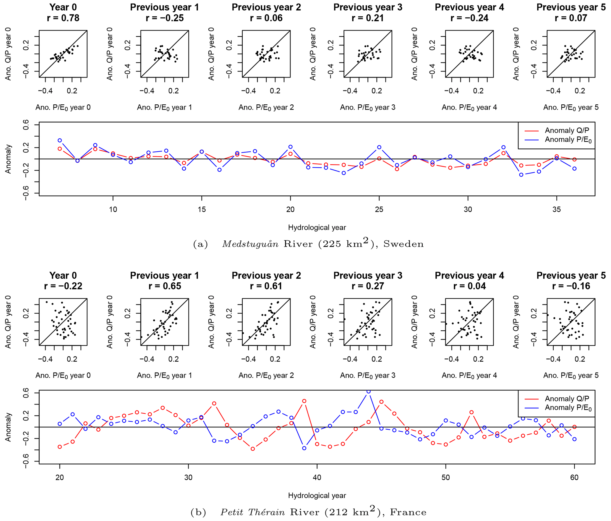
Figure 1 Elasticity analysis example of two catchments. No multi-year memory is detected on this Swedish catchment: a climatic anomaly $P/E_{\mathrm{0}}$ is directly affecting $Q/P$ of the same year but not later. In opposition, a multi-year memory is detected on this French catchment: the effect of a climatic anomaly $P/E_{\mathrm{0}}$ on the hydrology ($Q/P$) only starts after 1 year, before slowly decreasing (according to Pearson's r correlation values).

2.3 Parametrization of the CFCs

A CFC, as formulated in the Eq. (2), requires the calibration of n+1 values of ω. In order to limit the number of parameters and to avoid having to calibrate each ω value independently, we hypothesized (after many attempts that we cannot report here) that the shape of the CFC is similar to the shape of a Gamma distribution. This assumption is not uncommon among studies that focus on describing transit time distribution (see for instance: Kirchner et al., 2000, 2001; Dunn et al., 2010; Hrachowitz et al., 2010; Godsey et al., 2010; Tetzlaff et al., 2011; Heidbüchel et al., 2012; Berghuijs and Kirchner, 2017). This choice was also driven by visualizing all the plots obtained for our catchment set (e.g., Fig. 1). We found that a simple exponential parameterization would not be flexible enough because its maximum value will always be at the first time step, i.e., it does not allow to describe a lag between $Q/P$ and $P/E_{\mathrm{0}}$. A Gamma distribution (Eq. 3) requires the calibration of two parameters, a shape parameter α and a scale parameter β:

$$\begin{array}{}\text{(3)}& \mathit{\omega }\left(i\right)={\displaystyle \frac{i^{\mathit{\alpha }-\mathrm{1}}}{{\mathit{\beta }}^{\mathit{\alpha }}\mathrm{\Gamma }\left(\mathit{\alpha }\right)}}{e}^{-\frac{i}{\mathit{\beta }}},\end{array}$$

where Γ(α) is the Gamma function evaluated at α.

The different values of ω for each year i are estimated by integrating the Gamma density function between i and i+1. These ω values are rescaled so that their sum is equal to 1, according to the Eq. (2), and to provide the final values of the CFC. In summary, a CFC is built from the optimization of Eq. (2) using three parameters (ε₂, α and β).

For the sake of simplicity, before calibrating a CFC, we first fit a simple annual elasticity model (a zero-memory model), and use a statistical significance test (Student's t test with p value <0.01), to decide whether Eq. (2) improves significantly on Eq. (1). If the improvement is not significant, we conclude on the absence of multi-year memory for that catchment, and keep the simplest representation (that of Eq. 1). The objective function is a root mean square error (RMSE) of the $Q/P$ anomalies. It is used for the optimization of the parameter values and for this model selection. Parameters of both equations were calibrated using particle swarm optimization through the “hydroPSO” R package (Zambrano-Bigiarini and Rojas, 2013).

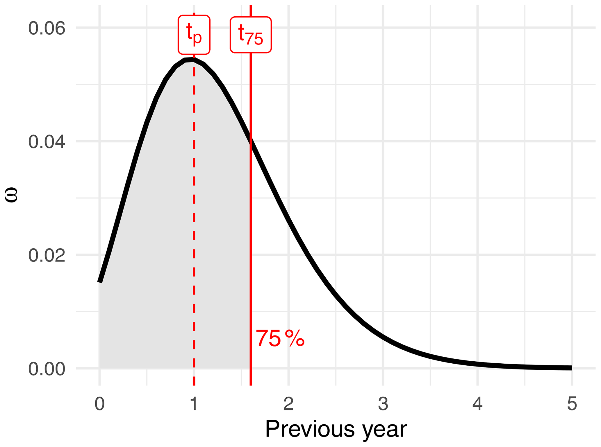
2.4 Summary of the CFCs

In order to quantify catchment memory, we assume that the Gamma distribution, from which ω values have been extracted, can be used to extrapolate a continuous temporal distribution of catchment memory. We extract two characteristic times from this temporal distribution (Fig. 2). Firstly, we extract the time when the temporal distribution is at its maximum value. This allows us to describe a possible lag between the climatic anomaly and the main resulting hydrological anomaly (called t_p). In addition, to describe the speed of memory loss, we extracted the time when the cumulative distribution reaches 75 % (called t₇₅), but any other percentage could be easily extracted in a similar way.

Figure 2 Extraction of two characteristic values from an example of a Gamma distribution.

2.5 Identification of hydroclimatic drivers of catchment memory

Based on the literature review of Sect. 1.5, we identified a few hydroclimatic descriptors that can explain catchment memory. Each catchment will be described with the average of the annual values of Q and P, E₀, $Q/P$ and $P/E_{\mathrm{0}}$. In addition, the percentage of the catchment area covered by lakes is used as a supplementary descriptor. This information is provided by SMHI for Swedish catchments (extracted from https://www.smhi.se/data/hydrologi/vattenwebb, last access: 26 June 2019). For France, the Lake Water Bodies according to the Water Framework Directive is used (extracted from https://geo.data.gouv.fr/fr/datasets/cc23e393dc05180892f2bf04f0be0423b62ebd86, last access: 25 May 2021). Finally, the contribution of groundwater is assessed by a baseflow index (BFI) calculated according to the work of Pelletier and Andréassian (2020a) where the baseflow is estimated from the outflow of a quadratic reservoir. The approach has two parameters (calibrated for each catchment): the reservoir capacity and the duration over which past effective precipitations filling this reservoir are taken into account. This baseflow filtering was performed with the associated “baseflow” R package (Pelletier et al., 2021).

The statistical distribution of each of these descriptors will be compared among three catchment memory classes: no multi-year memory, short multi-year memory and long multi-year memory. The first class corresponds to catchments for which the Student's t test (from Sect. 2.3) did not reveal a significant multi-year memory. The remaining catchments are split into two groups according to the median value of their memory in order to distinguish catchments with short multi-year memory and catchments with long multi-year memory.

3 Results and discussion

3.1 Is multi-year memory a rare phenomenon?

Approximately 80 % of the Swedish catchments and 89 % of the French catchments showed no significant multi-year memory (significant in terms of the aforementioned Student's t test): This shows that multi-year catchment memory is not the most common situation. We present in Fig. 3 the CFCs identified for the Swedish and French catchments separately. In Sweden, many of the catchments with multi-year memory exhibit a lag of 1 year (Fig. 3). This lag also appears in France where it sometimes reaches values of up to 3 years.

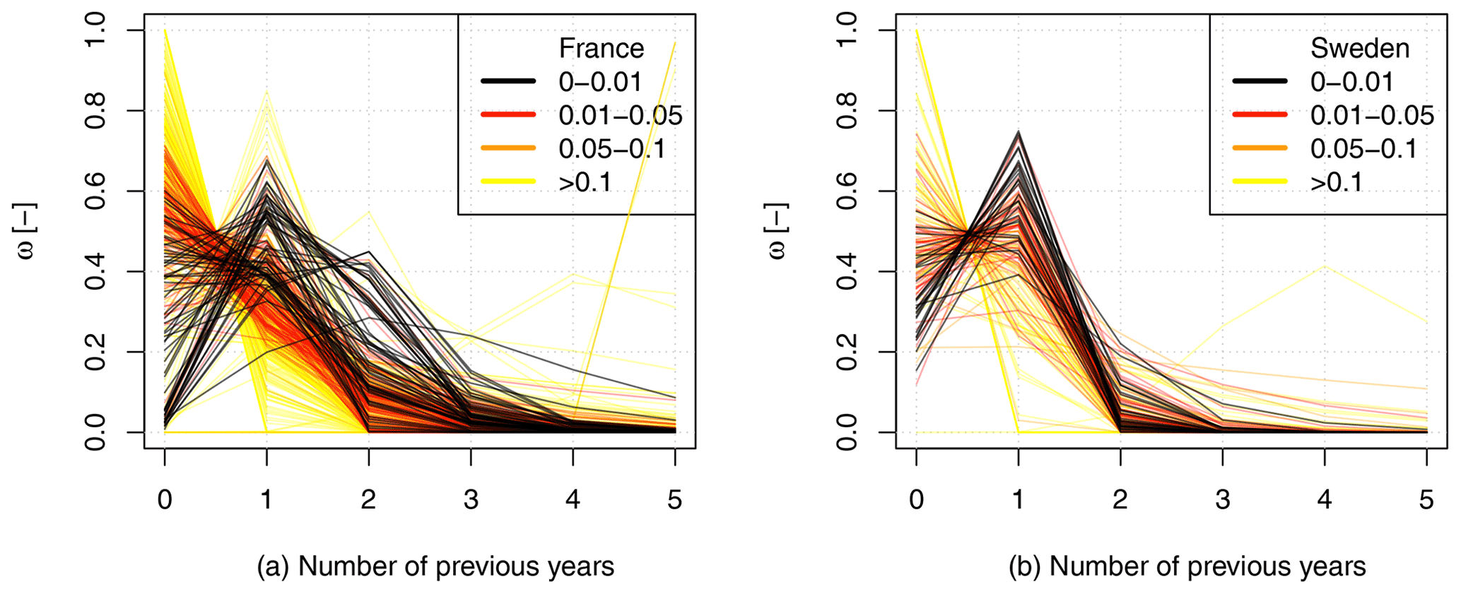
Figure 3 Catchment Forgetting Curves identified for the catchments on our French (a) and Swedish (b) dataset. The black lines represent the catchments where the multi-year CFC is very significant, and the color gradient represents, for the rest of the catchments, the p value of the t test.

In France, the weight of year 0 (ω₀) can frequently be equal to 0 (Fig. 3). This lag effect means that a climatic anomaly will not have an impact until the next year (as in the example presented in Fig. 1b). By contrast, Sweden rarely shows such an extreme temporal disconnection, and the climatic anomaly of year 0 is most of the time already affecting catchment yield during the current year.

In France, the calibration of the CFC sometimes yields a slow decrease, from year 0 to year 5, without any lag. But this shape does not really appear in Sweden, where the decrease in the memory is usually fast, with most ω values already becoming negligible after 2 or 3 years (Fig. 3). In France, the ω values become negligible after 4 or 5 years (which is why we retained 5 years as the maximum duration for the CFC).

3.2 Where do catchments exhibit a multi-year memory?

A spatial analysis of the catchments with significant multi-year memory already allows us to identify some spatial patterns (Fig. 4). In France, the Paris basin with its large chalk aquifer is the region where the most significant multi-year memory exists. In the rest of France, multi-year memory is generally not significant. In Sweden, long-term memory is mainly detected in the south of the country. Some hydroclimatic characteristics of these regions could explain these spatial patterns (see Sect. 3.3 below). No spatial pattern appears in snow-covered regions (e.g., the Alps and northern Sweden). This shows that snow melt affects mostly the seasonal memory with no significant impact on $Q/P$ over several years.

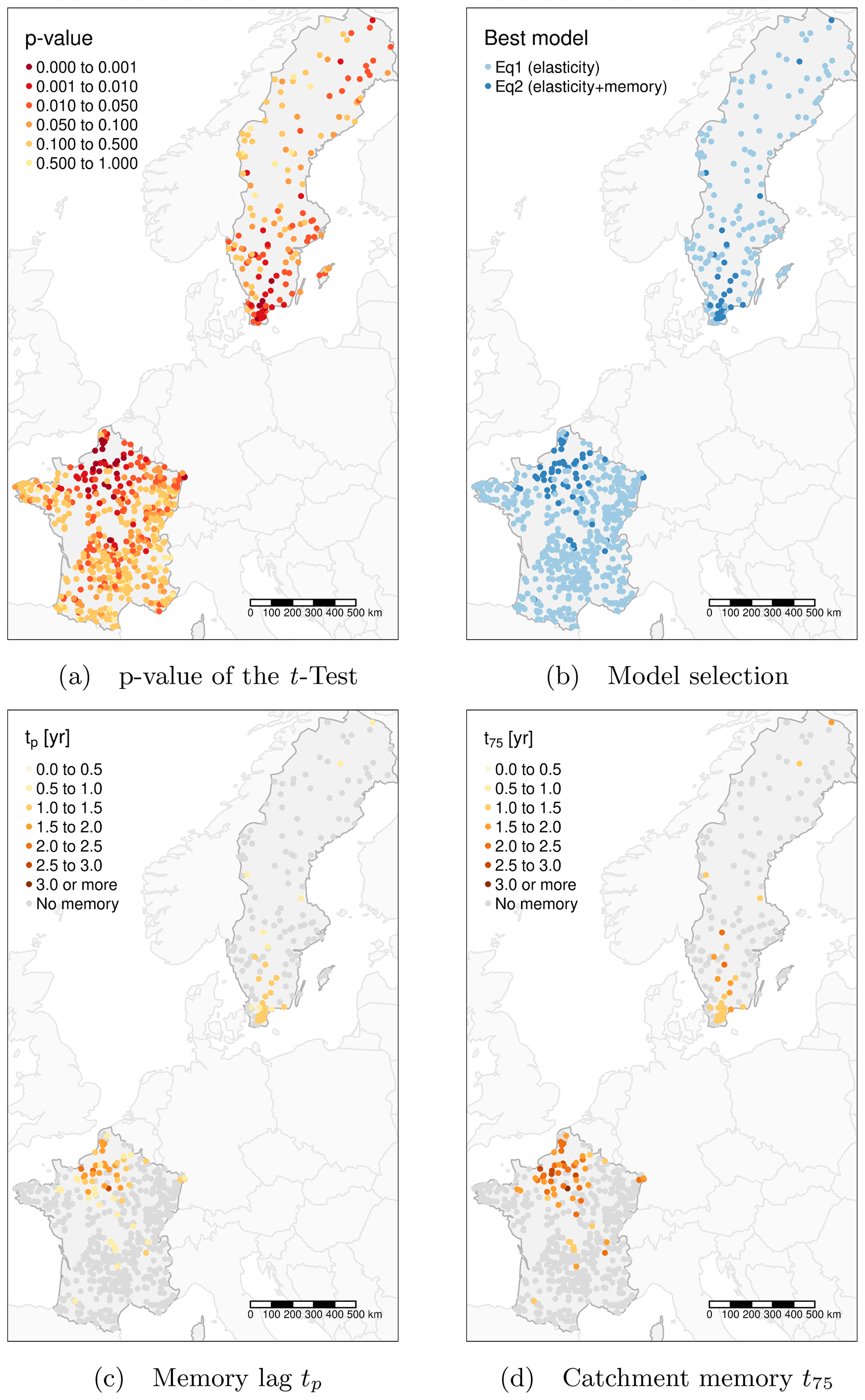
Figure 4 Spatial distribution of catchment memory over France and Sweden. Note that the model describing multi-year catchment memory (Eq. 2) is used only when the p value of the t test is below 0.01. Memory values are extracted from the Gamma distribution (see Sect. 2.4): t_p is the time when the Gamma density function is maximum, and t₇₅ is the time when the cumulative distribution reaches 75 %.

By extracting the quantile 75 % of the cumulated Gamma distribution (t₇₅, which we use to characterize the CFC, see Sect. 2.4), it is possible to quantify the duration of catchment memory. For these multi-year memory catchments, t₇₅ is often between 2 and 3 years in France, whereas it never exceeds 2 years in Sweden (Fig. 4).

3.3 Can multi-year memory be explained by hydroclimatic descriptors?

Figure 5 links catchment memory (t₇₅) to a few hydroclimatic characteristics commonly identified as the main drivers in the literature. Larger catchments tend to have longer memory in France, whereas in Sweden the memory does not seem to be related to catchment area.

For both countries, the memory increases under drier hydroclimatic conditions (as characterized by either lower discharge and precipitation, lower $Q/P$ or lower $P/E_{\mathrm{0}}$). However, the effect of potential evaporation does not appear to be clear. It thus seems that past climatic conditions have more influence on the hydrological behaviour of the driest catchments than on that of humid catchments. It can be hypothesized that under wetter conditions, water storage is renewed more often and the memory therefore tends to decrease.

In France, a higher BFI is associated with catchments with a longer memory. This confirms the predominant role of large aquifers in catchment memory. It also corroborates the spatial analysis of Fig. 4, where long memory is mainly located within the Paris basin where groundwater contributes significantly to total discharge. For France, this spatial organization is thus very consistent with the memory estimates of Pelletier and Andréassian (2020a).

In Sweden, the percentage of the catchment area covered by lakes (lake cover, Fig. 5) does not indicate a longer memory for catchments with larger lake cover. Compared with France, much of Sweden has thinner soils (as expressed by the available water capacity, Ballabio et al., 2016), which may account for a lower storage capacity and thus a shorter memory. Hydroclimatic characteristics with long memory in Sweden are consistent with catchments having higher seasonal prediction potential identified by Lopez et al. (2021) such as a high BFI and a low amount of precipitation.

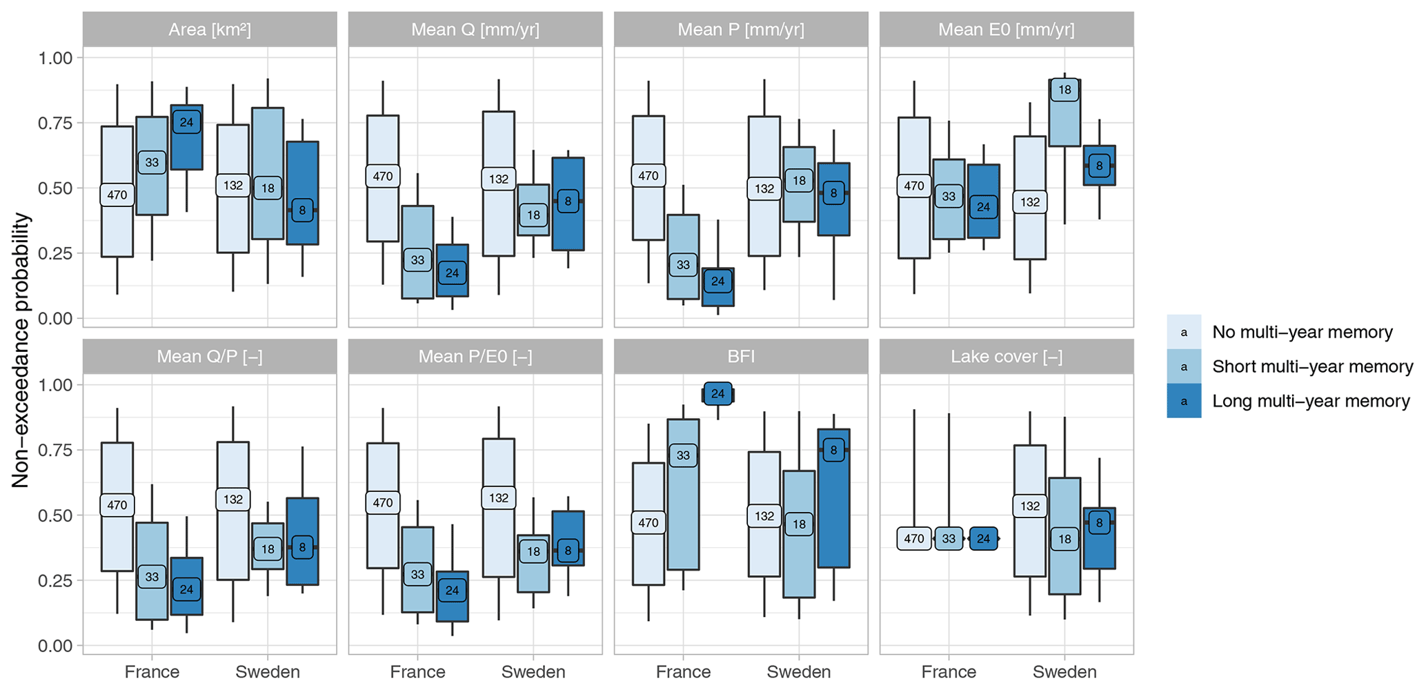
Figure 5 Distribution of hydroclimatic characteristics according to three classes of memory (described by t₇₅). The first class corresponds to catchments with no significant multi-year memory, the remaining catchments are split into two groups (shorter memory and longer memory) according to the median value of their memory. The numbers within each boxplot describe the number of catchments. The boxes are delimited by quantiles 0.25 and 0.75; whiskers by quantiles 0.1 and 0.9.

3.4 What do we miss in catchment elasticity analysis when not accounting for multi-year memory?

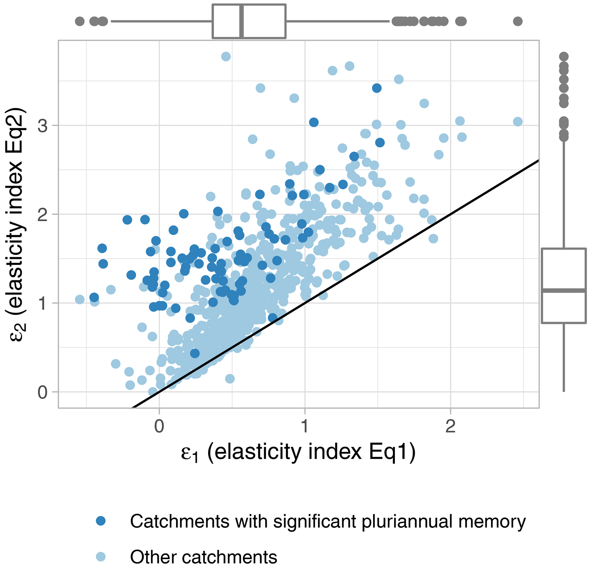
Equations (1) and (2) both quantify the elasticity ε in the relation between $Q/P$ and $P/E_{\mathrm{0}}$, but Eq. (1) does not account for multi-year memory effects, whereas Eq. (2) does. Figure 6 compares these two elasticity indices and highlights that the elasticity of Eq. (2) is always higher than the elasticity obtained with Eq. (1) and generally slightly exceeds the value of 1.

The numerical values of the elasticities obtained with Eqs. (1) and (2) should not be compared (the fact that one is lower than the other has no meaning). Equation (1) uses annual $P/E_o$ anomalies whereas Eq. (2) uses a weighted average value of past $P/E_o$ anomalies. The averaging of past $P/E_o$ anomalies will inevitably smooth the extremes and will give a value generally closer to zero (which is the long-term average value of $P/E_o$ anomalies). These lower anomalies of $P/E_o$ are logically compensated for by higher elasticity values during calibration (ε₂≥ε₁).

Figure 6 also shows that catchments with multi-year memory usually have higher relative differences between ε₁ and ε₂ (in the sense of distance to the bisector) than the rest of the catchments. This highlights the fact that, despite the numerical artifact previously discussed, the elasticity of catchments with multi-year memory is often under-estimated if this memory is not explicitly considered. A climatic anomaly will thus affect runoff yield more strongly than expected by Eq. (1), but with a delay.

By considering catchment memory, the elasticity values are thus changed. However, no strong relations were found between elasticity values and memory values (see Appendix A).

Figure 6 Comparison of elasticity indices found when ignoring multi-year memory effects (Eq. 1) and when explicitly accounting for them (Eq. 2) for all catchments (France and Sweden).

3.5 Can elasticity values be explained by hydroclimatic descriptors?

Similarly to catchment memory, we can try to link elasticity indices to some classic hydroclimatic characteristics. Figure 7 illustrates these relations for the elasticity indices of Eq. (2) (i.e., the equation accounting explicitly for the memory effect).

The relation between elasticity and catchment area is inverted between France and Sweden. In France, large catchments have greater elasticity, but in Sweden great elasticity is observed in smaller catchments. Our conclusion is that catchment size is not a first-order determining factor of memory and elasticity, and this likely reflects some more regional relation between catchment size and hydrology. For instance, specific discharge tends to increase with catchment size in Sweden, whereas it decreases in France (not shown here).

The stronger trends are found between catchment humidity and elasticity indices. Similarly to catchment memory (Fig. 5), elasticity increases with humidity-related indicators: lower humidity index $P/E_{\mathrm{0}}$, lower discharge and precipitation, higher E₀, lower $Q/P$. This suggests that water-limited catchments not only have a longer memory, but that their hydrological behavior is also more sensitive to climatic inputs. The low values of elasticity in wet areas can also be explained by the fact that the runoff yield, although generally higher, is less variable, thus leading to a lower slope in the $Q/P$ versus $P/E_{\mathrm{0}}$ relationship (Fig. 8).

Higher BFI values coincide with lower elasticity values in both France and Sweden. This suggests that a large contribution of groundwater attenuates the sensitivity to climatic anomalies. Even though these catchments have a longer memory of climatic anomalies, the impact of these anomalies is distributed and smoothed over the years. In Sweden, lakes also smooth the effect of climatic anomalies, but not as much as humid conditions or large baseflow contributions.

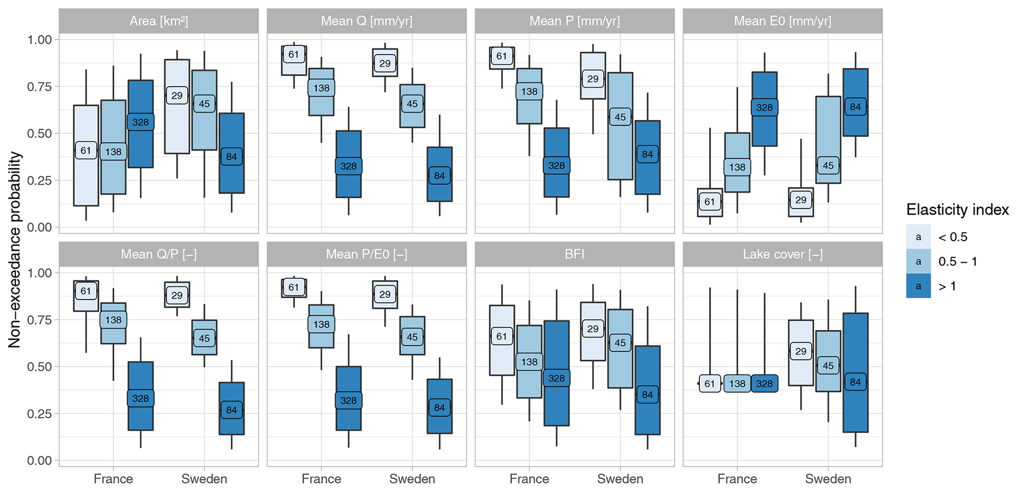
Figure 7 Distribution of hydroclimatic characteristics according to three classes of the elasticity index (ε₂) in Eq. (2). The numbers within each boxplot describe the number of catchments. The boxes are delimited by quantiles 0.25 and 0.75; whiskers by quantiles 0.1 and 0.9.

Figure 8 Comparison of the elasticity index (ε₂, Eq. 2) with the slope in the linear relation between $Q/P$ and $P/E_{\mathrm{0}}$ (a), and with inter-quartile differences of $Q/P$ values (b). Slopes can be visualized for each catchment through the segments. Segments are drawn between the two points defined by the first and third quartiles of these two ratios. A square root transformation is applied to both axes.

The elasticity is also quite well structured in space (Fig. 9). This spatial organization reflects the climatic conditions of each region, as already described by Fig. 7. The two elasticity indices (ε₁ and ε₂) generally have the same spatial patterns, except for the catchments with a significant multi-year memory. The very low elasticity values that they obtained with Eq. (1) (that can even be negative) were due to the impossibility of correctly linking $Q/P$ and $P/E_{\mathrm{0}}$ without considering the memory effect. Because it considers explicitly catchment memory, Eq. (2) yields elasticity values that are more coherent in space (and avoids the negative values that indicated a lack of hydrological understanding).

Figure 9 Comparison of elasticity index values obtained by optimizing Eq. (1) (which does not account for memory effects) and Eq. (2) (which does account for memory effects). The classes are delimited by quantile values to make a relative comparison of spatial patterns easier.

4 Conclusions

4.1 Synthesis

In this article, we proposed a new approach to quantifying catchment multi-year memory. We followed Ebbinghaus (1885) and defined Forgetting Curves, which represent how fast a catchment forgets past climatic inputs. These curves only require the knowledge of annual discharge data and climatic inputs: the precipitation–runoff relationship is analyzed through the classic concept of elasticity, linking the annual anomalies of runoff yield ($Q/P$) to the anomalies of humidity index ($P/E_{\mathrm{0}}$). In this work, we added a new dimension to the elasticity concept by also considering the past anomalies of the humidity index and by weighting these anomalies using a Gamma distribution, which shapes the CFC.

A first result is that only a limited percentage of catchments have a significant multi-year memory (about 15 % in our data set).

A second important result is that the catchments with significant multi-year memory are dominated by groundwater. In France, these “hypermnesic” catchments are underlain by well-known deep aquifer formations (e.g., the chalk aquifer of the northern part of the Paris basin). In Sweden, the expected effect of the lakes does not appear to be clear. As with snow, this memory seems to be essentially seasonal, with no detected multi-year impact. Catchment area does not seem to play a first-order role (we find different trends in France and Sweden).

A third meaningful result is that the humidity index appears to be one of the main drivers of catchment memory in both countries. This does not mean that dry catchments necessarily have a longer memory, but rather that a long memory only turns detectable on the drier catchments. Indeed, the memory requires dry periods to express itself. The elasticity indices were also well related to humidity, with humid catchments showing lower elasticity. Indeed, humid catchments tend not only to have a higher runoff ratio, but also a lower variance of this ratio, which leads to lower elasticity values.

Last, we show that not accounting for multi-year memory may yield elasticity indices with erratic values (that can even be negative). Introduction of the memory component produces a much more spatially coherent organization of the elasticity. Indeed, any analysis of the elastic relationship between precipitation and streamflow must take into account the potential lag between these two variables, even at the annual time step. If this temporal disconnection is not taken into account, the elasticity analysis may be biased and elasticity values tend to be underestimated.

4.2 Limits

Our methodology relies on a simplifying assumption where short-term and long-term memories are distinguished. It was thus tempting to quote Klemeš et al. (1981), who, at the end of their paper (where they discussed short- and long-memory models), wrote:

As a scientific hypothesis about streamflow series behavior, neither the short-memory nor the long-memory model can be falsified on the basis of historic flow records of a typical length. Hydrologically, they thus both remain, in Popper's sense, within the realm of metaphysics, and the choice between them is a matter of value judgment. The only arguments that can be advanced for either of them are operational and subjective: Occam's razor and lack of hard evidence to the contrary for short-memory models, hedging against a suspected possibility of a slightly higher risk for the long-memory ones.

In our case, we would argue that the behavior described in this paper contributes some “hard evidence” on the behavior of hydrological systems, without any unneeded complexity. We agree that a more comprehensive approach that would not need to distinguish between short and long memory (using a relatively arbitrary p value, Fig. 4) would probably be preferable, if it could be achieved with the same parsimony.

It would also be tempting to directly relate our CFC to distributions of travel time (see the discussion in Sect. 1.2). But this is clearly outside the scope of our method. We do not follow any water particle from its entry to its exit as a tracer would do. Thus, the values of memory that we obtained may not reflect water ages.

4.3 Perspectives

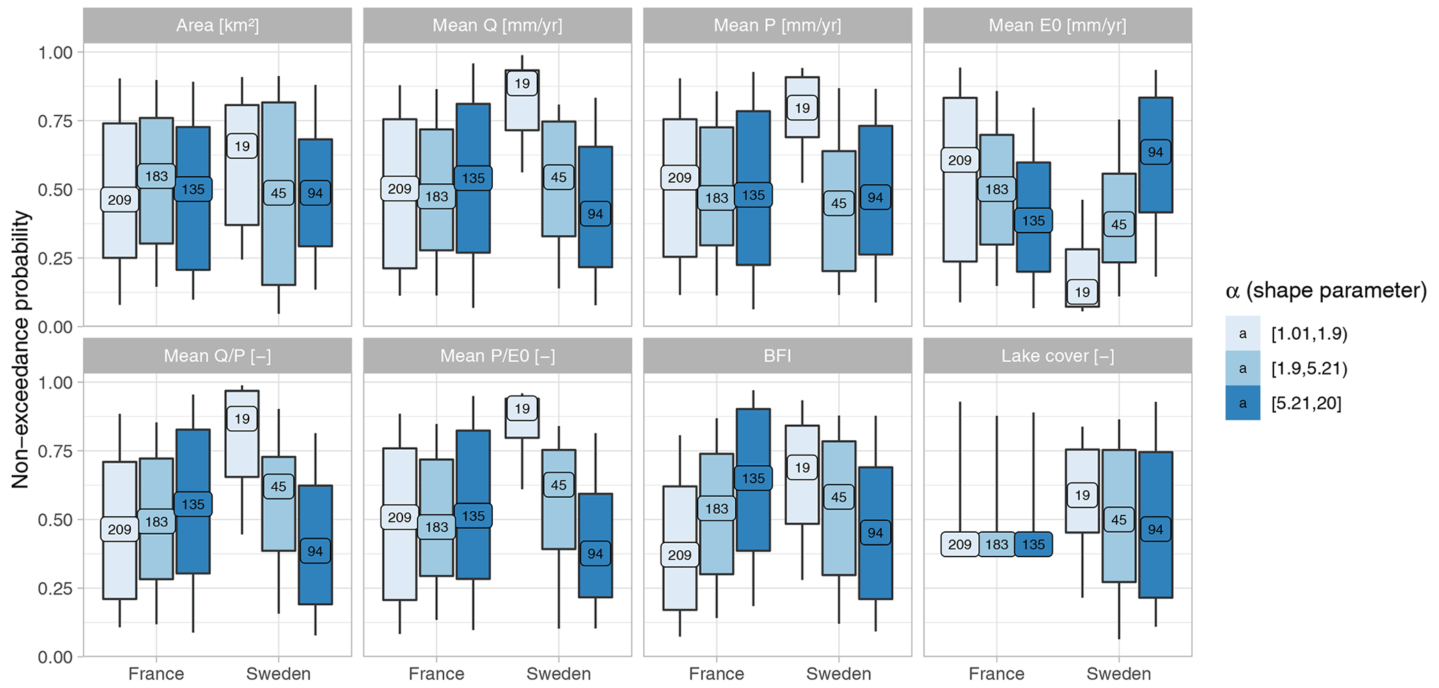
In order to be used operationally, it would be interesting to predict catchment memory without the need for model calibration against long time-series of discharge observation. An efficient regionalization of the approach could rely on defining relations between the characteristics of the CFC and hydroclimatic characteristics. This study shows that elasticity may be regionalized properly, as it is mainly driven by climatic conditions. However, the parameters of the Gamma distribution seem less easy to regionalize, especially the scale parameter β (see Appendix B). One perspective would be to better relate the two parameters of the Gamma distribution to catchment characteristics or to try other distribution assumptions that would allow for this more easily.

The parsimony of the proposed approach allows us to consider large-scale implementation on well-gauged territories. From a hydrological forecasting perspective, the maps thus produced can be used to better identify the predictability of the hydrological behavior of a catchment through the knowledge of past climatic inputs. From a changing climate perspective, they also provide an initial understanding of the sensitivity of watersheds to climatic anomalies and their effect on a multi-year time scale. Future work could also design dynamic CFCs by investigating how climate anomalies might change the shape of CFCs over time.

Catchment memory is fundamental for hydrological understanding, especially of regional hydrological processes. We need to learn more about this phenomenon for efficient water management and landscape planning. To better understand the causes of differences in catchment memory and elasticity, we recommend a more thorough analysis against physiographical conditions, including different catchment characteristics mentioned in Sect. 1.5. This could, for instance, be geomorphology, geology, vegetation, soil type and depth, aquifer interactions, groundwater levels, and human modifications (tile drainage, land degradation, reservoirs).

Appendix A: Relations between elasticity and catchment memory

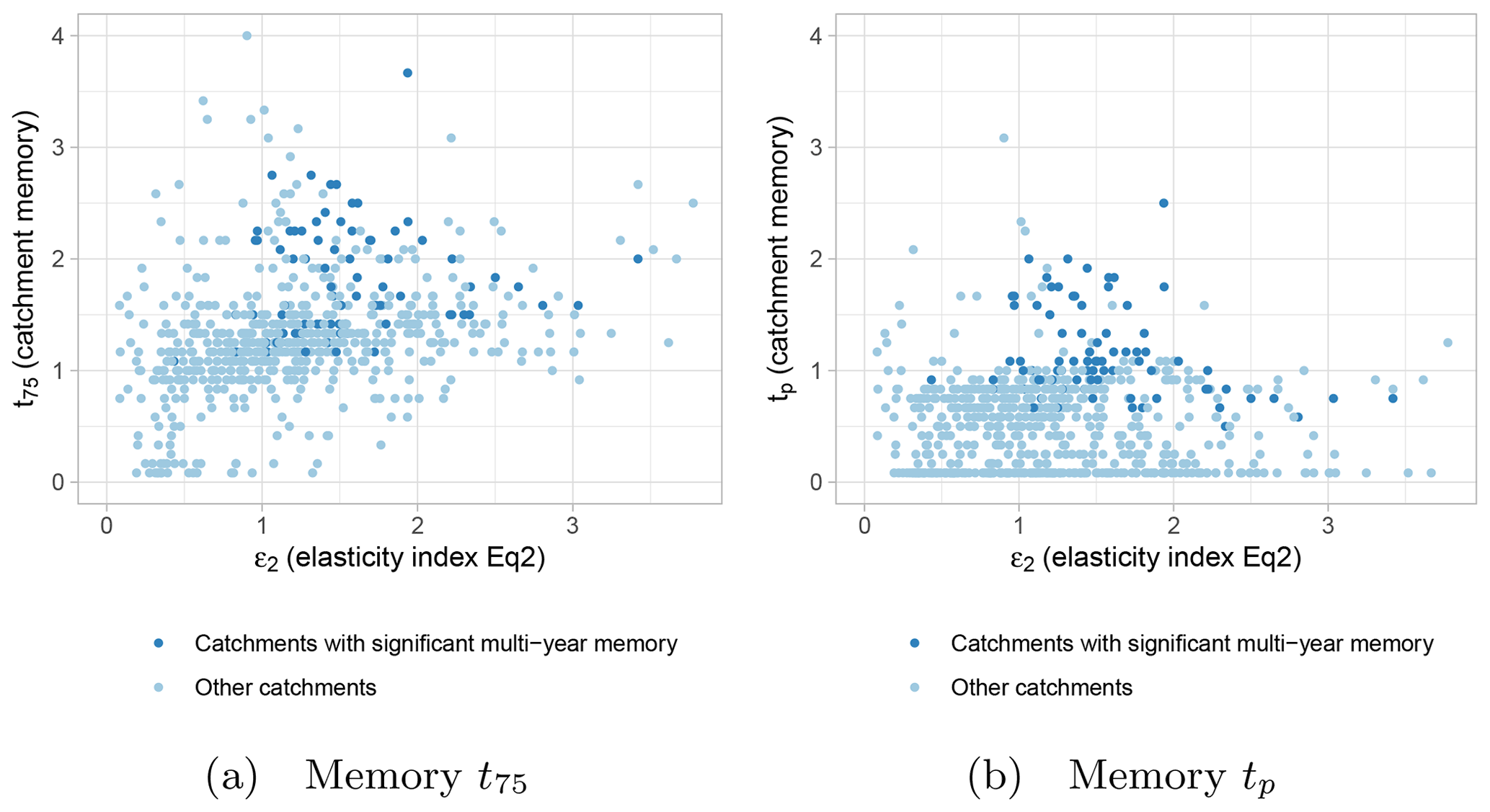
Figure A1 Relation between elasticity index (ε₂) of Eq. (2) and catchment memory assessed by t₇₅ and t_p.

One objective of this study is to disentangle catchment memory from catchment elasticity. This appendix illustrates that no strong relations were found between these two indexes, neither for catchments with nor for catchments without multi-year memory.

Appendix B: Regionalization of Gamma distribution parameters

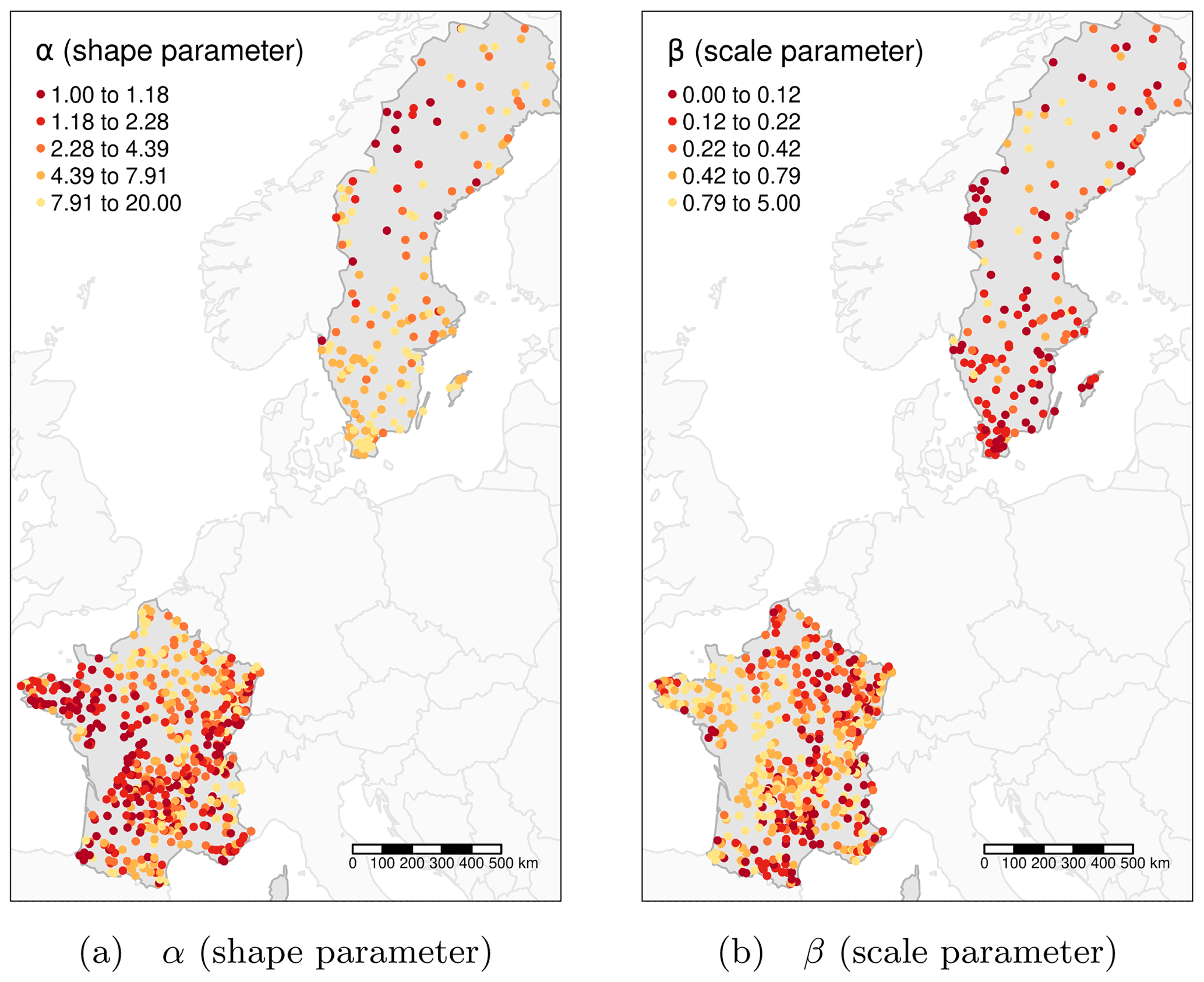
In this work, we assumed that the CFC can be described by a Gamma distribution. This appendix provides the spatial visualization of the two parameters of this Gamma distribution (α and β) optimized for each catchment (Fig. B1). Figures B2 and B3 illustrate the challenge of regionalizing these CFCs, with opposite relationships between France and Sweden when relating these parameters to hydroclimatic characteristics.

Figure B1 Map of the parameters of the Gamma distribution (Eq. 3) calibrated inside Eq. (2). The classes are delimited by quantile values.

Figure B2 Distribution of hydroclimatic characteristics according to three classes of the shape parameter α of the Gamma distribution (Eq. 3) calibrated inside Eq. (2). The classes are delimited by quantile values. The numbers within each boxplot describe the number of catchments.

Figure B3 Distribution of hydroclimatic characteristics according to three classes of the scale parameter β of the Gamma distribution (Eq. 3) calibrated inside Eq. (2). The classes are delimited by quantile values. The numbers within each boxplot describe the number of catchments.