the Creative Commons Attribution 4.0 License.
the Creative Commons Attribution 4.0 License.
 | 27 Apr 2022
Investigating the response of leaf area index to droughts in southern African vegetation using observations and model simulations
Stephen Sitch
Danica Lombardozzi
Julia E. M. S. Nabel
Hao-Wei Wey
Pierre Friedlingstein
Hanqin Tian
Bruce Hewitson
In many regions of the world, frequent and continual dry spells are exacerbating drought conditions, which have severe impacts on vegetation biomes. Vegetation in southern Africa is among the most affected by drought. Here, we assessed the spatiotemporal characteristics of meteorological drought in southern Africa using the standardized precipitation evapotranspiration index (SPEI) over a 30-year period (1982–2011). The severity and the effects of droughts on vegetation productiveness were examined at different drought timescales (1- to 24-month timescales). In this study, we characterized vegetation using the leaf area index (LAI) after evaluating its relationship with the normalized difference vegetation index (NDVI). Correlating the LAI with the SPEI, we found that the LAI responds strongly (r=0.6) to drought over the central and southeastern parts of the region, with weaker impacts (r<0.4) over parts of Madagascar, Angola, and the western parts of South Africa. Furthermore, the latitudinal distribution of LAI responses to drought indicates a similar temporal pattern but different magnitudes across timescales. The results of the study also showed that the seasonal response across different southern African biomes varies in magnitude and occurs mostly at shorter to intermediate timescales. The semi-desert biome strongly correlates (r=0.95) to drought as characterized by the SPEI at a 6-month timescale in the MAM (March–May; summer) season, while the tropical forest biome shows the weakest response (r=0.35) at a 6-month timescale in the DJF (December–February; hot and rainy) season. In addition, we found that the spatial pattern of change of LAI and SPEI are mostly similar during extremely dry and wet years, with the highest anomaly observed in the dry year of 1991, and we found different temporal variability in global and regional responses across different biomes.
We also examined how well an ensemble of state-of-the-art dynamic global vegetation models (DGVMs) simulate the LAI and its response to drought. The spatial and seasonal response of the LAI to drought is mostly overestimated in the DGVM multimodel ensemble compared to the response calculated for the observation-based data. The correlation coefficient values for the multimodel ensemble are as high as 0.76 (annual) over South Africa and 0.98 in the MAM season over the temperate grassland biome. Furthermore, the DGVM model ensemble shows positive biases (3 months or longer) in the simulation of spatial distribution of drought timescales and overestimates the seasonal distribution timescales. The results of this study highlight the areas to target for further development of DGVMs and can be used to improve the models' capability in simulating the drought–vegetation relationship.
- Article
(6245 KB) - Full-text XML
-
Supplement
(1681 KB) - BibTeX
- EndNote


Drought can be described as a natural occurrence whereby the natural accessibility of water for a region is beneath the normal state over a long period of time (Xu et al., 2015). Globally, it is considered one of the world's most important climate risks, with significant environmental, social, and ecological impacts on different sectors (e.g. agriculture, forestry, and hydrology) and human lives (Naumann et al., 2018). Increasing trends in the occurrence and severity of drought in West Africa and the Mediterranean have huge impacts on water resources and agriculture (Sultan and Gaetani, 2016). In southern Africa, a region regarded as a climate hotspot because of the projected impacts of climate change on its numerous endemic vegetation, an understanding of these impacts is important for mitigation options in managing future drought events. Therefore, it is important to examine drought impacts on vegetation and evaluate how this is simulated in models.
Drought is a frequent occurrence in southern Africa and has enormous impacts on vegetation in the region. For instance, drought has resulted in a significant loss of biomes and the death of plants (Masih et al., 2014; Hoffman et al., 2009). It is reported that there has been a significant loss of vegetation cover over the region over the last 30 years (Driver et al., 2012; DEA, 2015). Drought has also impacted the speciation of vegetation thereby causing significant changes to the region's rich biomes through the lack of formation of new species or even the growth of species with underdeveloped morphological and physiological characteristics (Hoffman et al., 2009). Drought-induced vegetation loss has both ecological and socioeconomic consequences for human lives. For instance, studies have shown that food security in the region is threatened due to the continual mortality of vegetation (FAO, 2000; Müller et al., 2011). Other studies (e.g. Wang, 2010; Khosravi et al., 2017) have also reported that southern Africa could lose more than USD 200 billion of its GDP (gross domestic product) from the effects of drought on vegetation. The enormous impacts on vegetation have thus made it imperative to investigate how vegetation might respond to different drought intensities at varying timescales.
In order to monitor and quantify drought characteristics, drought indices are used (Wilhite and Glantz, 1985). Drought indices, including the SPI (i.e. the Standardized Precipitation Index), standardized water-level index, and standardized anomaly index, are derived from a single hydrological variable, which is rainfall (Kwon et al., 2019). Other indices such as the Palmer drought severity index, multivariate standardized drought index, and standardized precipitation evapotranspiration index (SPEI) combine two or more variables related to other atmospheric or soil and environmental conditions that may predispose a plant to water stress (Palmer, 1965; Vicente-Serrano et al., 2010; Hao and AghaKouchak, 2013). Among the drought indices, the SPI is the most widely used because of the adjustable timescale and its relatively simple calculation (McKee et al., 1993). It is also recognized as appropriate for use in southern Africa (Hoffman et al., 2009). However, the SPI has a significant shortcoming, which is that its computation uses only rainfall without considering the effect of other meteorological variables in the development of drought occurrence (Teuling et al., 2013). In order to address this shortcoming, the SPEI was developed for drought monitoring, and it is regarded as being a more suitable drought index in the region to investigate the spatiotemporal scale of drought (Ujeneza and Abiodun, 2014). SPEI is computed from the difference between potential evapotranspiration (PET) and rainfall (Vicente-Serrano et al., 2010). PET can be computed using different methods such as the Hargreaves (HG) and Penman–Monteith (PM) methods. Although studies (e.g. Vicente-Serrano et al., 2010) have found that the PM method captures drought better than HG, other studies (e.g. Lawal et al., 2019a) showed that this difference is negligible over southern Africa.
Many studies have used different indices to quantify observed drought, characterize vegetation, and study drought effects on the productiveness of vegetation across different timescales. Several studies (e.g. Vicente-Serrano and National Center for Atmospheric Research Staff, 2015; Zhang et al., 2012; Lawal et al., 2019a, b) have shown that the satellite-derived normalized difference vegetation index (NDVI) is one the most important indicators of vegetation health and greenness. These studies applied NDVI in examining drought impacts on global vegetation biomes. However, other studies (Gitelson, 2004; Santin-Janin et al., 2009) have argued that, while the NDVI is a true proxy for vegetation trends, its potential saturation makes it difficult to fully estimate biomass. In addition, because the NDVI parameters are not well calibrated and often missing from the models, simulated NDVI can be biased. Due to its high correlation with NDVI, the leaf area index (LAI) is instead used to characterize vegetation conditions (Fan et al., 2008; Zhao et al., 2013). Although the LAI is an important vegetation proxy, it is rarely considered in the estimation of drought impacts on vegetation. Thus, quantifying the response of the LAI to drought over southern Africa is important for understanding the processes that modulate ecosystem services produced by vegetation which are crucial for human survival (Melillo, 2015).
Previous studies have also evaluated the performance of coupled climate models in simulating the response of vegetation to drought. For instance, Lawal et al. (2019a) reported that an ensemble of the Community Earth System Model (CESM) showed biases in response simulation of vegetation to drought. This was attributed to the parameterizations of the land component (i.e. community land model – CLM) which poorly simulated observed NDVI. Given the poor replication of the vegetation response to drought by a coupled climate model, there is a need to examine land-only models and whether they might better capture the drought–vegetation relationship when the atmospheric forcings are derived from observations. The present study used dynamic global vegetation models (DGVMs) to study the vegetation response to drought, as little is known about how the LAI response to drought is simulated by DGVMs. The choice of DGVMs is because of their capability to simulate a mostly accurate carbon exchange between the atmosphere and vegetation ecosystems (Lu et al., 2011).
The aim of this study is to investigate the response of LAI to droughts in southern African vegetation using observations. We also examined how well the responses are represented in model simulations. We used satellite-derived and simulated LAI to quantify vegetation responses to drought. We characterized the spatiotemporal extent of drought and its severity using the SPEI and then assessed the influence of drought using the LAI from satellite data and model simulations.
2.1 Data
In this study, we used satellite-calculated (hereafter, observed LAI/observation-based LAI) and simulated LAI and satellite-derived NDVI, with gridded observation and reanalysis climate data sets. The gridded observation climate data sets include precipitation and maximum, mean, and minimum temperature. These data were obtained from CRU (i.e. the Climate Research Unit; Mitchell and Jones, 2005; Harris et al., 2014). These are global monthly data which have as spatial resolution and span the 1901–2019 period. Here, we used the CRU data for the period 1982–2011 to compute observed drought indices (i.e. SPEI) to characterize the spatiotemporal severity of drought. CRU is a gridded observed data set, which was used because of its suitable spatial and temporal resolutions. Previous studies (e.g. New et al., 2000; Otto et al., 2018; Harris et al., 2020) have shown that there is a good and robust agreement between the observation network and CRU over most parts of southern Africa. We should note that sparseness and missing data generally affect the correlation between CRU and station data in the region. Furthermore, with respect to the interannual variability, CRU robustly captures the climate factors in southern Africa. The major exception is with the long-term trend of precipitation, particularly over the Western Cape province of South Africa and wetter than normal conditions over the same province. These limitations do not affect the validity of our results because we are looking at below-normal precipitation and temperature.
The reanalysis climate data we used are the CRUJRA, which is a combination of CRU and the Japanese Reanalysis data (JRA) (University of East Anglia Climatic Research Unit; Harris et al., 2020). It is a 6 h land surface, gridded data with a spatial resolution . CRUJRA was used to compute reanalysis drought indices and used for model simulations. Here we aggregated CRUJRA to monthly samples and used the data at the same spatial and temporal resolution as CRU.
For the satellite vegetation indices, first, we used the third generation of NDVI (hereafter, NDVI3g) from the Global Inventory Modelling and Mapping Studies (GIMMS), spanning the period from 1981–2015, with a biweekly temporal resolution and a spatial resolution of about 8 km (Pinzon and Tucker, 2014; National Center for Atmospheric Research Climate Data Guide, accessed 2019). Here, we used the data for the period 1982–2011. Furthermore, we used the third generation of the GIMMS LAI (LAI3g), which also spans the period 1981–2015 and has a biweekly temporal resolution and the same spatial resolution as GIMMS3g. The LAI data had been processed (at source) using a set of neural networks which were first trained on the highest quality and post-processed MODIS LAI and fraction of photosynthetically active radiation (FPAR) products and advanced very high resolution radiometer (AVHRR) GIMMS NDVI3g data for the overlapping period (2000 to 2009). The trained neural networks were then used to produce the LAI3g and FPAR3g data sets (Mao and Yan, 2019). For the study, LAI3g was also used for the period 1982–2011. We note that GIMMS LAI and the NDVI, used in this study, are two different indices. The LAI was post-processed using different data (MODIS LAI, FPAR, and AVHRR NDVI) for the period of 2000–2009. The GIMMS LAI product is superior here over the GIMMS NDVI, which is due to the information derived from the MODIS LAI. The additional properties on GIMMS LAI by MODIS differentiate the index from the NDVI. Thus, it was necessary to investigate how the two indices differ. In addition, other studies (Forkel et al., 2013; Schaefer et al., 2012; Rezaei et al., 2016; Lawal et al., 2019a) have investigated how well satellite-derived LAI estimates actual and ground-measured LAI.
The simulated monthly LAI data were obtained from 11 DGVMs which are part of the TRENDY version 7 model (Sitch et al., 2008; Le Quéré et al., 2014). These DGVMs are CABLE-POP (Haverd et al., 2018), CLM (Oleson et al., 2013), CLASS-CTEM (Melton and Arora, 2016), DLEM (Tian et al., 2015), JSBACH (Mauritsen et al., 2018), LPX (Lienert and Joos, 2018), OCN (Zaehle et al., 2011), ORCHIDEE (Goll et al., 2017), SURFEX (Joetzjer et al., 2015), JULES (Clark et al., 2011), and VISIT (Kato et al., 2013). LAI from the models have a monthly temporal resolution spanning the period from 1901–2017. We selected these DGVMs because they have been run with a similar protocol (S3 simulations) and forcing data sets (i.e. CRUJRA).
2.2 Methods overview
2.2.1 Evaluation of DGVMs and the relationship between NDVI and LAI
The relationship between the NDVI and LAI was evaluated by computing the grid cell spatiotemporal correlation between GIMMS NDVI and GIMMS LAI. The spatiotemporal correlation between GIMMS LAI and simulated LAI from individual DGVMs was also calculated. This was necessary to show whether LAI is an appropriate estimator of NDVI and how well the models simulate the LAI in the region. Furthermore, we made comparisons of the seasonal values of observed and modelled LAI. We note that the lack of available of data makes it difficult to compare GIMMS LAI and actual LAI. Nevertheless, the GIMMS LAI has been evaluated and agrees well with observations in other regions (Fan et al., 2019).
The climatology of observed and simulated climatic variables, as well as LAI over six major biomes in southern Africa for the period 1982–2011, were computed. These biomes are semi-desert, Mediterranean, dry savanna, moist savanna, temperate grassland, and tropical forest (Fig. 1; Sinclair and Beyers, 2015; Lawal et al., 2019a, b).
2.2.2 Description of drought
For the present study, we adopted the definition of meteorological drought, “which is described as a period (e.g. a season) during which there is a deficit in the magnitude of precipitation in a particular area compared to the long-term normal” (Palmer, 1965; Wilhite and Glantz, 1985). The deficit in magnitude of precipitation compared to the long-term normal is mostly accounted for by temperature and less by humidity, wind, or other variables. Here, we used meteorological drought because it does not make any presumptions about soil characteristics or runoff. In addition, it is acknowledged to be a primary component in the depletion of vegetation productiveness and the reduction in biomass (Vicente-Serrano et al., 2010). Previous studies (Vicente-Serrano et al., 2006; Vicente-Serrano, 2013) have also used meteorological drought in the investigation of drought impacts on biomass and vegetation productiveness.
2.2.3 Drought computation and correlation with LAI
The analyses include calculating drought (i.e. SPEI) using CRU data over a 30-year period (1982–2011) for different drought timescales. The drought timescale can be described as the aggregation of the temporal duration (Vicente-Serrano et al., 2010). SPEI is an index that is used to quantify drought (see Table 1). Therefore, the quantified values of the index give the state of drought in a space. Our definition and approaches follow numerous previous studies (Vicente-Serrano, 2013 Vicente-Serrano, 2013; Khosravi et al., 2017; Zhao et al., 2013; Hao and AghaKouchak, 2013).
Table 1Definition of drought thresholds based on the SPEI scale.
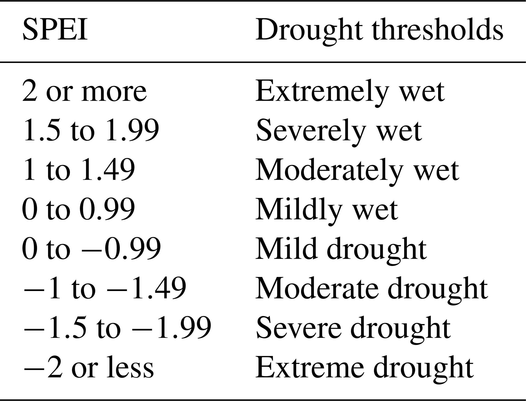
Sources: Wang et al. (2014) and modified as shown in Lawal (2018).
A time series of the evolution of drought for the 30-year period was plotted. The present study extends the time frame for understanding drought impacts from 1982 to 2011, mainly because there were frequent droughts in the 2005–2011 window (Masih et al., 2014). The time frame was then extended back to cover a 30-year period to be long enough to cover the impacts of climate change, which is particularly important considering that southern Africa experiences more frequent droughts with impacts exacerbated by climate change. This information is important for considering adaptation measures and understanding the role of climate change.
The drought index, SPEI, is calculated from the deduction between precipitation (P) and potential evapotranspiration (PET) as follows:
where D values represent a measurement of water deficit or surplus aggregated at different timescales. D values are obtained through aggregation over individual timescales which span 1 to 24 months (i.e. 1, 3, 6, 9, 12, 15, 18, 21, and 24 months). The timescales were calculated by including the past values of the variable. For example, a timescale of 15 months suggests that input from the preceding 15 months, which includes the present month, was used for calculating SPEI (Beguería et al., 2014). “For the 1-month timescale, only the current month data [are] used for the calculation. The D values were standardized by assuming a suitable statistical distribution (e.g. gamma, log-logistic). The log-logistic distribution was used to standardize the D values in this study” (see also Lawal et al., 2019a). For more details on the timescale computation, please see Vicente-Serrano et al. (2010; https://rdrr.io/cran/SPEI/man/spei.html, last access: January 2010). PET is computed from maximum temperature, minimum temperature, and mean temperature, using the HG technique (e.g. Vicente-Serrano et al., 2012; Beguería et al., 2014; Stagge et al., 2014).
We note that the PET in the SPEI was computed using the Hargreaves (HG) method rather than Penman–Monteith (PM) because the data (e.g. vapour pressure and maximum and minimum humidity) required for computing PM over southern Africa are sometimes missing or not available at the needed gridded spatial resolutions and time span. Although PM is considered better in most regions, Lawal et al. (2019a) showed that the variation between the PM and HG is negligible for the southern African region. The study only considered observed SPEI_PM, which was obtained from https://spei.csic.es/database.html (last access: January 2010), and not modelled SPEI_PM, due to the unavailability of simulated data required for its computation. Other studies (e.g. Beguería et al., 2014) have also found that there is an insignificant contrast in the strength of PM and HG for reproducing their divergence on measured variables such as vegetation indices. We should also note that the SPEI (unlike SPI or the Palmer drought severity index – PDSI) is the most appropriate index for measuring drought in southern Africa, as it accounts for the effect of the evaporative demand from the atmosphere in drought monitoring (Vicente-Serrano et al., 2010; Ujeneza, 2014). In addition, the SPEI is reported to be able to identify the geographical and temporal coverage of droughts (Vicente-Serrano et al., 2010; Ujeneza, 2014).
We deseasonalized GIMMS LAI by transforming the monthly LAI series per pixel to symbolize the standardized deviations from the extended mean. This was to make the sequence of LAI commensurate to SPEI (Vicente-Serrano, 2013) and eliminate the impact of periodicity on vegetation response. We note that the SPEI is intrinsically deseasonalized.
In order to reconcile the difference in the spatial resolutions of CRU and GIMMS, we regridded the data to the same spatial resolution using the bilinear interpolation method. We then computed the correlation per grid cell between SPEI (based on CRU) and deseasonalized LAI over the 30-year period at the different drought timescales using Pearson correlations. We then compared the spatial distribution of maximum (peak) correlation and the comparable timescales of drought for observed SPEI. Our analyses consider the periods at which LAI responds to the presence/absence and the severity of drought. This is referred to as the drought timescale in the study.
Next, we investigated correlations at each grid cell between the drought (from reanalysis – CRUJRA) and an ensemble median of deseasonalized modelled LAI from individual DGVMs. The peak (maximum) correlations and equivalent timescales from the complete 1- to 24-month timescales were mapped for the ensemble median over the 30-year period. We used the ensemble median because of its lower sensitivity to independent outliers (Reuter et al., 2013). In summary, we calculated the model ensemble drought from the median from individual members' drought indices. The interannual variation in drought impacts on LAI by individual DGVMs was also calculated for different timescales. We also examined the observed and ensemble mean of the simulated LAI response to drought across latitudes.
In summary, CRU was used to compute observed drought while CRUJRA was used to calculate modelled drought because it is what was used to force the models. This will allow for easy observation and model comparisons.
Similar to Lawal et al. (2019a), we calculated the seasonal mean for four seasons, i.e. (a) December, January, and February (DJF), (b) March, April, and May (MAM), (c) June, July, and August (JJA), and (d) September, October, and November (SON), from the correlations of monthly series of drought and LAI. These were computed from correlating the monthly series (12 series per year) per pixel of GIMMS LAI and each monthly series of a 1- to 24-month drought (SPEI) series over the 30-year period with the Pearson correlation. The same technique was used for the model ensemble. In simpler terms, we calculated the correlations (12 sequences in a year) of monthly LAI to the monthly sequences of a 1- to 24-month SPEI using 30 years of data. Subsequently, the seasonal mean of these correlations was calculated. The peak correlations and drought timescales of the models were calculated over six major biomes in southern Africa, namely (Fig. 1) temperate grassland, tropical forest, moist savanna, dry savanna, semi-desert, and Mediterranean vegetation. These regions were selected because of their relative importance and are most affected by drought.
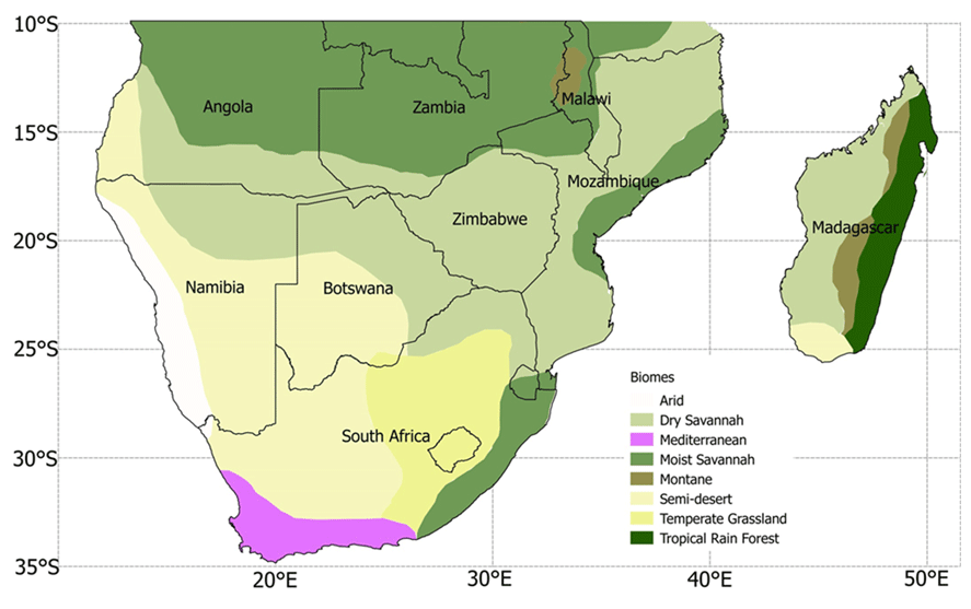
Figure 1Major vegetation biomes in southern Africa (adapted from UNEP, 2008, Sinclair and Beyers, 2015, and Lawal et al., 2019a, b). The black lines indicate political boundaries.
Finally, the impacts of extreme events (wet and dry years) at different time periods were compared, and the comparison of global and regional responses to drought across biomes for the period 1982–2011 was investigated.
3.1 Grid cell correlations between NDVI and LAI
Figure 2 illustrates the relationships between the NDVI and LAI for observations, as well as the comparison between observed and modelled LAI. There is a strong linear relationship between observed NDVI and LAI (Fig. 2a). The correlation (0.94) is high between both variables, and the standard deviation is low (0.005). The standard deviation being referred to is for GIMMS LAI and individual DGVMs, as well as GIMMS LAI and GIMMS NDVI. From the figure, a log-like shape can be seen, where NDVI grows faster when LAI is low (<0.2) and becomes saturated when LAI goes higher (>0.3). A linear regression of the data shows a slope of 2.15. The low standard deviation indicates that the values from the two indices are close. Although there is a good agreement between observed NDVI and LAI, the 1:1 line shows that the data sets are not exactly equal.
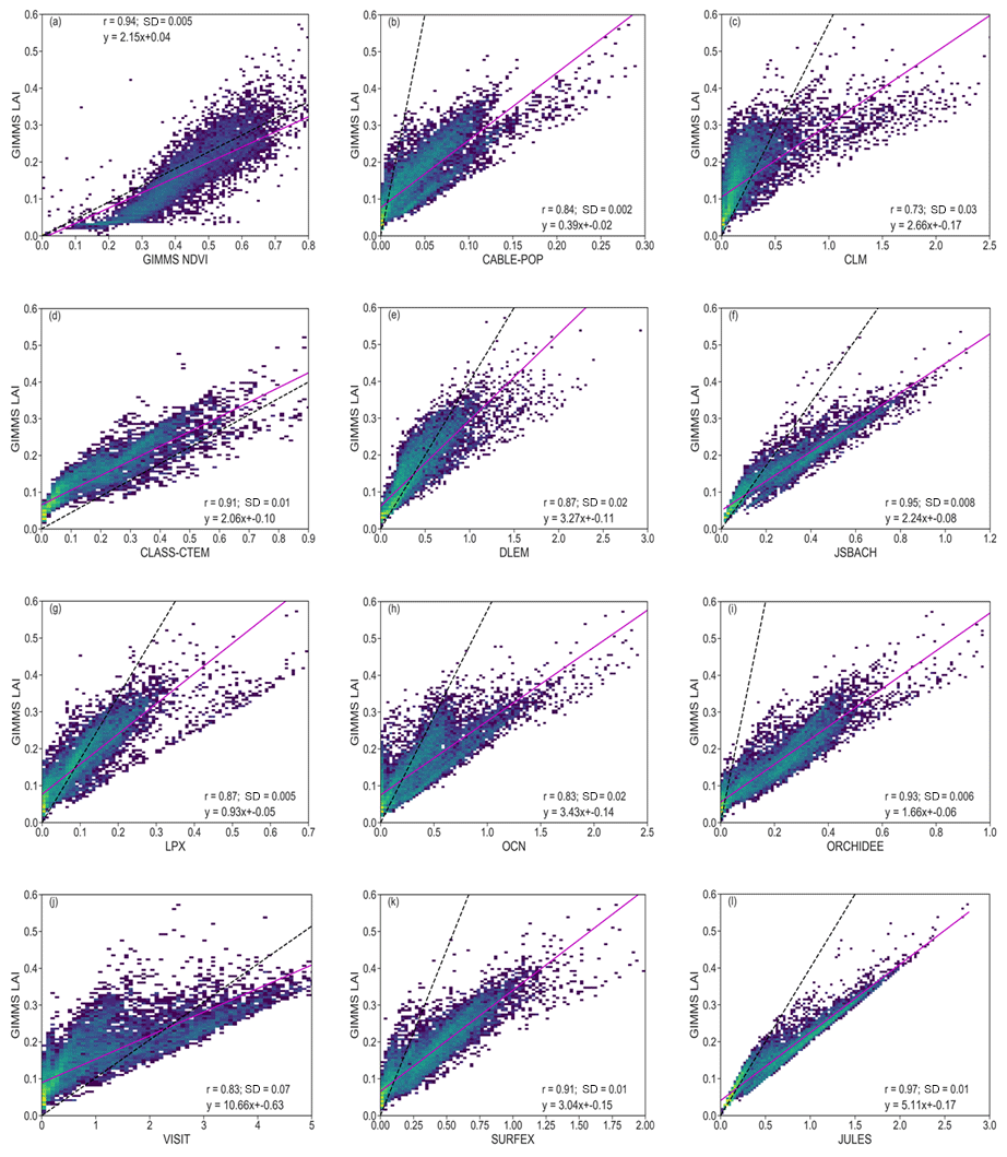
Figure 2Scatterplots of correlations between vegetation indices (observation and model) for the period 1982–2011 over southern Africa. Inset values indicate the correlation coefficient (r) and standard deviation (SD) between GIMMS LAI and GIMMS NDVI, as well as GIMMS LAI and modelled LAI. The colour represents each grid cell. The pink solid line is the linear regression, while the dashed black line shows the 1:1 line. The unequal x axes are to visualize the detailed data for the models.
Furthermore, there is good agreement between the observed and the simulated LAI (Fig. 2). JULES has the highest correlation (0.97) with observation (Fig. 2l). CLM has the weakest (0.73) correlation with the observations (Fig. 2c). DLEM and LPX have the same correlation coefficient value of 0.87 with the observation (Fig. 2e and g). The positive relationships between simulated and observed LAI indicate a general applicability in investigating the model's performance of vegetation response to drought. It also shows that the correlation is strong enough to compare how the LAI reacts to drought in the ensemble. An aggregation of the observation along the gradient of simulated LAI shows that most of the models have similar slopes to the observation.
3.2 Seasonal and interannual variations in observed and modelled LAI
The comparison of seasonal and interannual variation of the observed and modelled LAI is given in Fig. 3. The model shows a stronger positive bias in JJA and SON in comparison to the summer and winter months and a negative bias over the tropical forest region of Madagascar (Fig. 3a–d). In addition, the models mostly overestimate the seasonal patterns of LAI in some regions during DJF and JJA and underestimate LAI in MAM and SON (Fig. 3e–l). Over most parts of the region, there is a strong correlation and good agreement between the observed and modelled LAI in DJF, MAM, and JJA, although it is weaker in SON (Fig. 3m–t). The strong correlation is more prevalent in JJA than other seasons (Fig. 3s), while it is weakest in the southern parts of the region. However, the correlation is largely negative over Angola in DJF and SON (Fig. 3q and t). Furthermore, the correlations between the model and observed LAI is weaker in deseasonalized data (hereafter deseas. correlation; Fig. 3m–p) than in original data (hereafter orig. correlation; Fig. 3q–t), thereby showing the effects of seasonal patterns on time series data. With respect to the period, 1982–2011 (hereafter annual), the correlation between the modelled and observed LAI are different for deseasonalized and original data (Fig. 3u and v). For the former (Fig. 3u), there is a gradient in the correlation across the region, with higher values in central and southern parts than in Angola and Madagascar. However, with the original LAI data (Fig. 3v), the correlation is very high (about 0.85) and more prevalent, except in eastern Madagascar and the Western Cape province of South Africa.
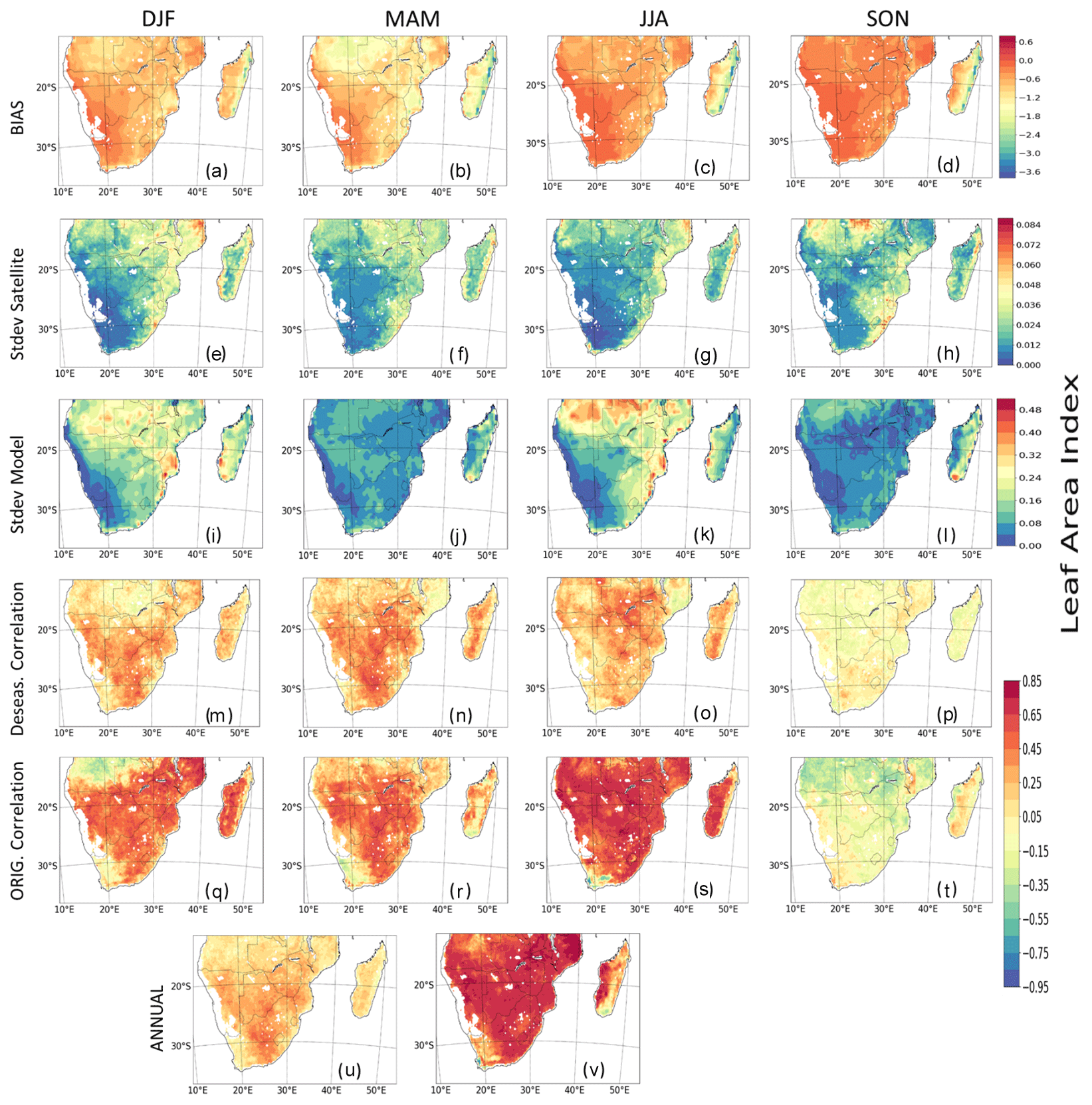
Figure 3Spatial seasonal distribution and interannual variability (IAV) of satellite-calculated and modelled LAI (multimodel mean) over southern Africa. Panels (a–d) show the difference (bias). Panels (e–h) and (i–l) show their standard deviation (SD). Panels (m–p) show the correlations between deseasonalized GIMMS LAI and modelled LAI. Panels (q–t) show their correlations for original GIMMS LAI and modelled LAI. Panels (u) and (v) show correlations between GIMMS LAI and modelled LAI but for the period 1982–2011. The interannual variability for observed and modelled LAI for the period 1982–2011 is shown in Fig. S8.
3.3 Climatology of observed and simulated climate variables and LAI
This section compares the seasonal cycle of observational (CRU and CRUJRA) climate variables and observed and simulated LAI from GIMMS LAI and TRENDY models, respectively. Precipitation and temperature are seasonally variable, and their climatologies are mostly similar. For example, precipitation is higher in MAM and DJF over many of the biomes, except in Mediterranean vegetation, where precipitation is higher in JJA (Fig. 4a, d, g, m, and p). The wettest month occurs over the TF (i.e. tropical forest biome) where the precipitation is about 350 mm. Conversely, during the dry season (JJA), there is little rainfall in the biome, although it experiences some precipitation June and July. Over the Mediterranean vegetation (Fig. 4j), a winter (JJA) rainfall region, rainfall variability is lower and is mostly dry in DJF and SON. Similarly, the highest minimum and maximum temperature in the region is observed in the DJF season, where the highest temperature value exceeds 30 ∘C. Over the tropical forest biome, although the distribution pattern of precipitation and temperature are similar for most months, they differ during June and July. The pattern of precipitation and temperature distribution generally differs over the Mediterranean vegetation. The pattern of temperature and precipitation from CRUJRA follows CRU, although the ensemble spread is much narrower (Fig. 4c, f, i, l, o, and r). The spatial patterns of the climate variables from CRU and CRUJRA are shown in Fig. 5. CRUJRA simulates the pattern of precipitation over southern Africa well (Fig. 5a and b) as CRU, although it shows some biases in magnitudes and for minimum temperature (Fig. 5g and h).

Figure 4Annual cycle of observed climate variables (precipitation in millimetres per month; maximum, minimum, and mean temperature in degrees Celsius) and LAI for observation and multimodel mean (TRENDY) across six southern African biomes for the period 1982–2011. The annual cycle of the LAI for individual models is shown in Fig. S5.
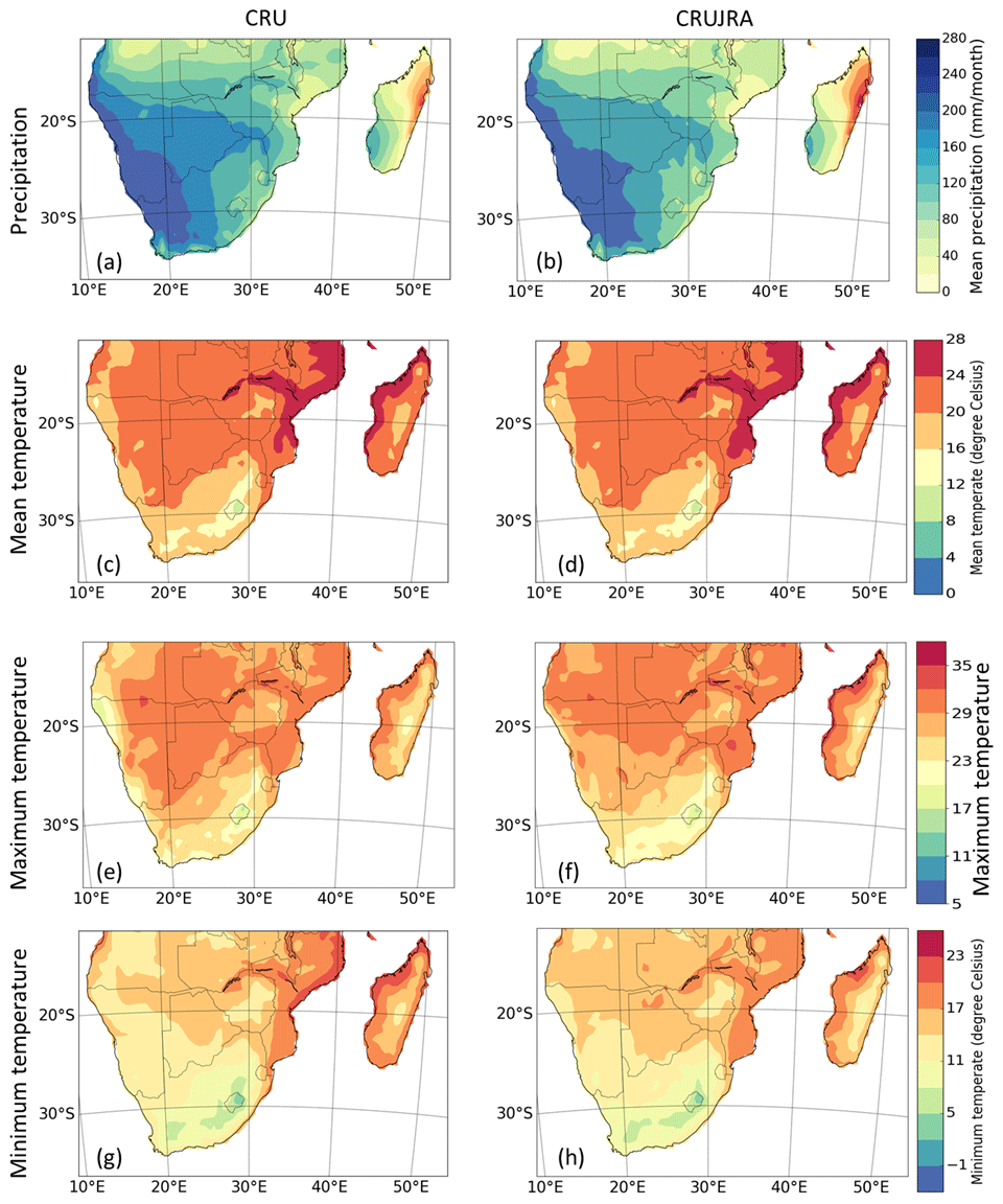
Figure 5Spatial distribution of precipitation, mean temperature, maximum temperature, and minimum temperature over southern Africa in CRU and CRUJRA for the period 1982–2011.
There is not a strong seasonality for LAI, with maximum observed LAI values being less than 4 in all biomes. The models reproduce the climatology of LAI over the southern African biomes well, with a few exceptions (Fig. 4b, e, h, k, n and q). For instance, the models simulate the drop in LAI over the semi-desert, temperate grassland, tropical forest, dry savanna, and moist savanna biomes in JJA. The highest increase in observed LAI occurs over the tropical forest in April, although the models simulate a decrease in LAI over tropical forest during this time. On the other hand, the lowest amount (less than 0.1) of LAI is observed in September, and this occurs over the semi-desert biome. Observations typically fall within the range of the model ensemble. In addition, the distribution pattern of the simulated LAI is similar to the observation in most biomes except in the Mediterranean and tropical forest biomes. The LAI pattern also follows that of the climatic variables, although the former lag. The lag effect is accounted for in this study and is known as the drought timescale.
3.4 The evolution of drought in southern Africa
Figure 6 shows the evolution of observed SPEI in southern Africa between 1982 and 2011. Here, drought indices from CRUJRA are not included because a preliminary investigation showed close magnitudes for drought indices computed from CRU and CRUJRA. We note that CRU was used to calculate SPEI for the observation, while simulated SPEI was computed with CRUJRA.
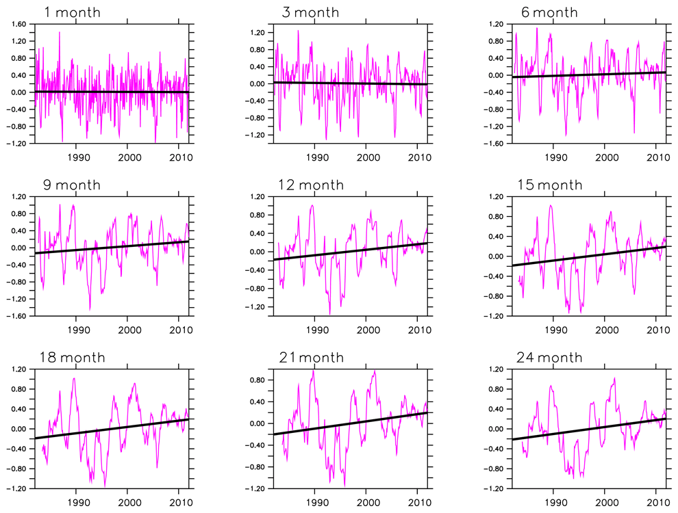
Figure 6Evolution of SPEI in southern Africa for the period 1982–2011. The trend is significant at the 90 % confidence interval for all timescales.
There is interannual, seasonal, and decadal variability in the drought indices during dry and wet conditions over southern Africa. Although 1-, 3-, and 6-month SPEI indicate no trend in wet or dry spells, they show the intensity of drought events for the 30-year period (Fig. 6a–c). The highest magnitude of the drought is captured by a 1-month SPEI while the lowest is shown in a 21-month SPEI. The severity of the drought intensity is similar for all SPEI (i.e. 1- to 24-month SPEI). The magnitude of the severity is on the y axis of the 1- to 24-month SPEI.
We note an increasing trend in SPEI (9 to 24 months). Tables 2 and 3 illustrate when droughts occurred and the severity of the droughts within the 30-year period. They also show, however, that droughts were most frequent and intense in the second decade, thus, indicating how climate change is expected to increase the frequency and severity of droughts.
Table 2Characteristics of drought occurrence for a 1- to 24-month drought timescale for the first decade (1982–1991), second decade (1992–2001), and third decade (2002–2011).
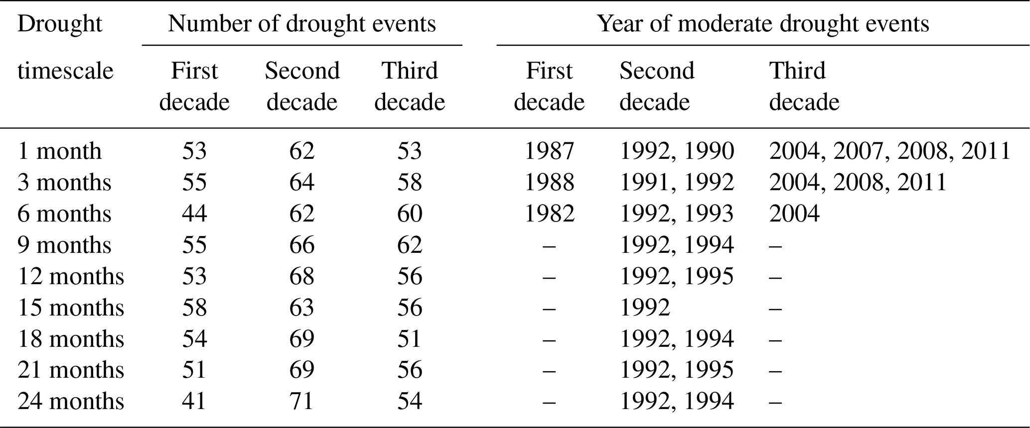
Table 3Statistics of the severity of drought for 1- to 24-month drought timescale for first decade (1982–1991), second decade (1992–2001), and third decade (2002–2011). SD is the standard deviation, and max is the highest magnitude of drought occurrence.

3.5 Spatial distribution of LAI response to drought and the timescales
Figure 7 presents the spatial distribution of the peak correlation between the SPEI and the LAI and the timescales at which the correlation occurs. This is to show the magnitude of response of LAI to drought in southern Africa and the length of the period for the response.

Figure 7Spatial distribution of peak correlation between drought (SPEI) and LAI over the region of southern Africa in the observation and in the model ensemble median for the period 1982–2011. Panels (a) and (c) show the peak correlation per pixel, which is independent of the timescale and the month of the year. Panels (b) and (d) indicate the timescales at which the peak correlation between SPEI and LAI is found. Areas with no significant correlation are white.
Observations show that southern African LAI can respond fairly strongly to droughts (peak correlation magnitudes of between 0.4 and 0.6), though the response is much weaker (r<0.4) in eastern Madagascar, Angola, and parts of South Africa (Fig. 7a). The TRENDY multimodel median generally overestimates the observed magnitude of the LAI to drought response (Fig. 7c). Peak correlations for the models seem to be much stronger, i.e. in the 0.6–0.8 range for most of the regions. In addition, over the arid areas of Namibia, models simulate a LAI, while observations depict no measurable LAI, indicating that models simulate the LAI in areas where observations show no measurable LAI.
The multimodel median has a drought timescale that is mostly longer than the observations (Fig. 7b and d). For instance, the drought response of simulated LAI occurs mostly over a longer time period (6- and 9-month timescale) than in the observation over eastern Madagascar. Over the southern areas of Madagascar and central Zambia, the multimodel median overestimates the drought timescale. Over the central areas of South Africa and Mozambique, simulated LAI responds at intermediate (9-month) timescales. In comparison, similar drought timescales for the observation and the model ensemble median are shown in parts of Angola.
3.6 Latitudinal distributions of LAI response to drought and the timescales
The present study investigated and discussed the implications of drought on different vegetation/biome types across latitudes in the region. Here, we stratified the LAI response to drought based on latitude because we intend to investigate and identify the shift in the response based on the vegetation types across the latitudinal belt.
While the pattern of the latitudinal distribution of the LAI response to drought is identical across different timescales, the magnitudes generally differ (Fig. 8). The response is much weaker (less than 0.15) for the 1-month timescale than for other timescales. The strongest response is observed at a 6-month timescale between latitudes of 25 and 30∘. The model ensemble mean generally agrees with the pattern of the observed LAI–SPEI correlations across all the timescales. However, the magnitudes differ from the observation. The modelled correlation is stronger than observations for the longer (6 months or more) timescales. This means that the models are oversimplifying how the LAI responds to drought by neglecting other climate factors, such that, in models, LAI only correlates to the water deficit (SPEI). Furthermore, there is an offset between the observation and model mean, which is consistent across most of the timescales, perhaps due to the strong memory of the some of the models.
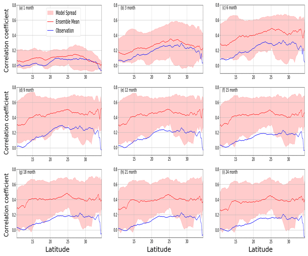
Figure 8Mean correlation (observed and multimodel ensemble) of annual LAI and SPEI for 1982–2011 across latitudes over southern Africa for 1- to 24-month timescales.
3.7 Response of LAI to droughts across seasons
Observations show similar correlations between LAI and drought across all seasons in the biomes (Fig. 9). For the dry savanna, which is one of the most climate-impacted biomes in the region, LAI response to drought is strong, the correlation is as high as 0.8 in MAM season, and it occurs at a 12-month timescale. The correlations between drought and LAI are also very strong in other seasons over the same biome and occur at 6- and 12-month drought timescale, except over the Mediterranean vegetation, where the response occurs at 18 months in the DJF season. Similarly, the peak correlations between drought and LAI are strong across the other biomes. With the exception of the tropical forest biome, the drought timescale is at longer time periods (>6 months).
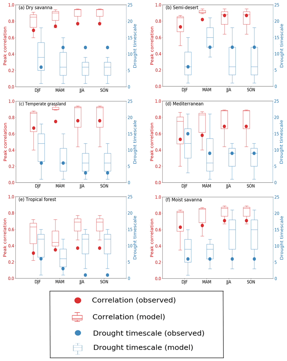
Figure 9Seasonal correlations of drought (SPEI) and LAI across six southern African biomes. The values on the left axis show the peak correlation in observation and TRENDY models. The values on the right axis indicate the corresponding drought timescale.
The model ensemble generally overestimates correlations across the biomes in different seasons. While the correlation magnitude remains mostly larger than the observation, models nonetheless simulate a closer correlation with observation in some biomes and seasons. For instance, over Mediterranean vegetation, models simulate a fairly good response of LAI to drought in all seasons. Furthermore, in nearly all other biomes, the ensemble spread overlaps with the observations. In addition, simulations mostly overestimate the drought timescale, except over dry savanna. A possible reason for why the difference in the timescale for dry savanna was underestimated may be because phenological triggers for dry savannah vegetation types respond differently to environmental variables, which the models do not capture. The African dry savanna region is characterized by rapid vegetation changes due to fire, land use, among others, and senescence for prolonged dry periods (Rahimzadeh-Bajgiran et al., 2012; Zhu and Liu, 2015), which may have contributed to the underestimation in the response of the models. Similarly, models have different representations of fire, which could also indirectly contribute to the underestimated model responses to drought.
3.8 Interannual variation in the model simulation of the drought impacts on LAI
Table 4 shows the correlations between observed mean SPEI and LAI for the period 1982 and 2011 and simulations by individual DGVMs across different timescales. Unlike Fig. 7, which shows the peak correlations, the table shows the mean correlation for the 30-year period.
Table 4Model simulation of mean SPEI and LAI correlations between 1982 and 2011. The asterisk (*) indicates the model with the lowest mean correlation.
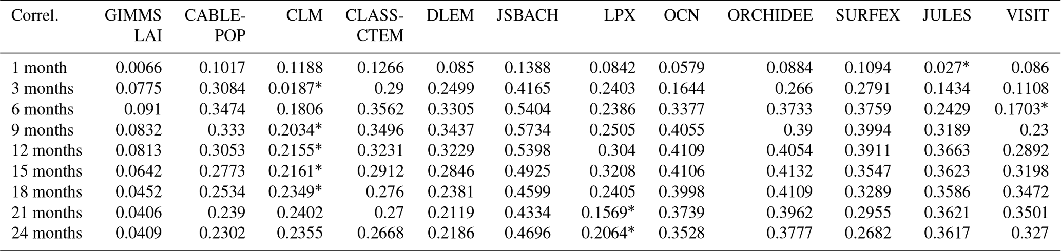
There is variation in the interannual simulation of LAI response to drought across different timescales by individual models. For instance, on the 1-month timescale, JULES simulates the lowest correlation value while JSBACH shows the highest correlation value. Furthermore, JSBACH simulates the highest correlation value for most of the timescales, while CLM simulates the lowest correlation values for most (3, 9, 12, 15, and 18 months) of the timescales. A possible reason for the weak performance of CLM may be its representation of the canopy construction of the plant functional types (PFTs) and of its foliage clumping representation. In addition, CLM is limited in its simulations of vegetation with regards to transpiration, due to the rooting depth, among others (Dahlin et al., 2020). Furthermore, CLM does not simulate savanna ecosystems well but instead uses a combination of grasses, shrubs, and trees. There are also some problems (such as an unusual green-up in the dry season) identified with deciduous stress responses (Dahlin et al., 2015).
3.9 Impacts of extreme events on LAI
The impacts of extreme events on LAI are shown in Fig. 10. The objective was to discuss the impacts and compound influences of extreme events on LAI during extremely hot/dry and wet years. Here, extreme events are the wet (2000, 2010, and 2011) years, i.e. the periods with precipitation higher than normal, and the dry (1983, 1984, and 1991) years, which include the periods of very high dry spells. To achieve this, we used the anomaly of precipitation, SPEI, and LAI relative to the long-term mean. The anomaly was computed as a difference between a particular extremely dry or wet year and 30-year mean representing dry and wet conditions. The anomaly is the magnitude of impacts added by the extreme event in a particular year. The spatial pattern of the changes in LAI, SPEI, and precipitation were then plotted. Our analyses follow Pan et al. (2015). Furthermore, we computed the pattern correlation coefficients (r) between the LAI and climate variables for each extremely dry and wet year. The statistical significance of the coefficients was also calculated. The goal of this is to ascertain whether the sign of the anomaly of the variables correspond in the same locations on two different maps. In order to determine the significance of correlation coefficient, we performed the linear regression t test (i.e. LinRegTTest). This finds the best line of fit among a set of data points. It also checks the quality of the fit by carrying out a t test on the slope, thus testing the null hypothesis that the best fitted line is 0, suggesting that there is no correlation between two variables, since an association with a slope of zero implies that one variable does not affect the other. Therefore, if the p value is not sufficiently low, then we do not have sufficient data to accept relationship between the variables. For this study, we used a significance level of 5 % i.e. α=0.05, which is the most commonly used value in life and biological sciences. We then tested the hypothesis on whether the p value is less than the significance level (α=0.05), which is our null hypothesis. In cases where that is the case, we rejected the null hypothesis and concluded that there is adequate evidence that there is a significant linear relationship between the variables i.e. LAI–SPEI and LAI–precipitation. In cases where the p value is greater, we do not reject the null hypothesis, since there is not enough evidence to conclude on the significance of correlation coefficients.
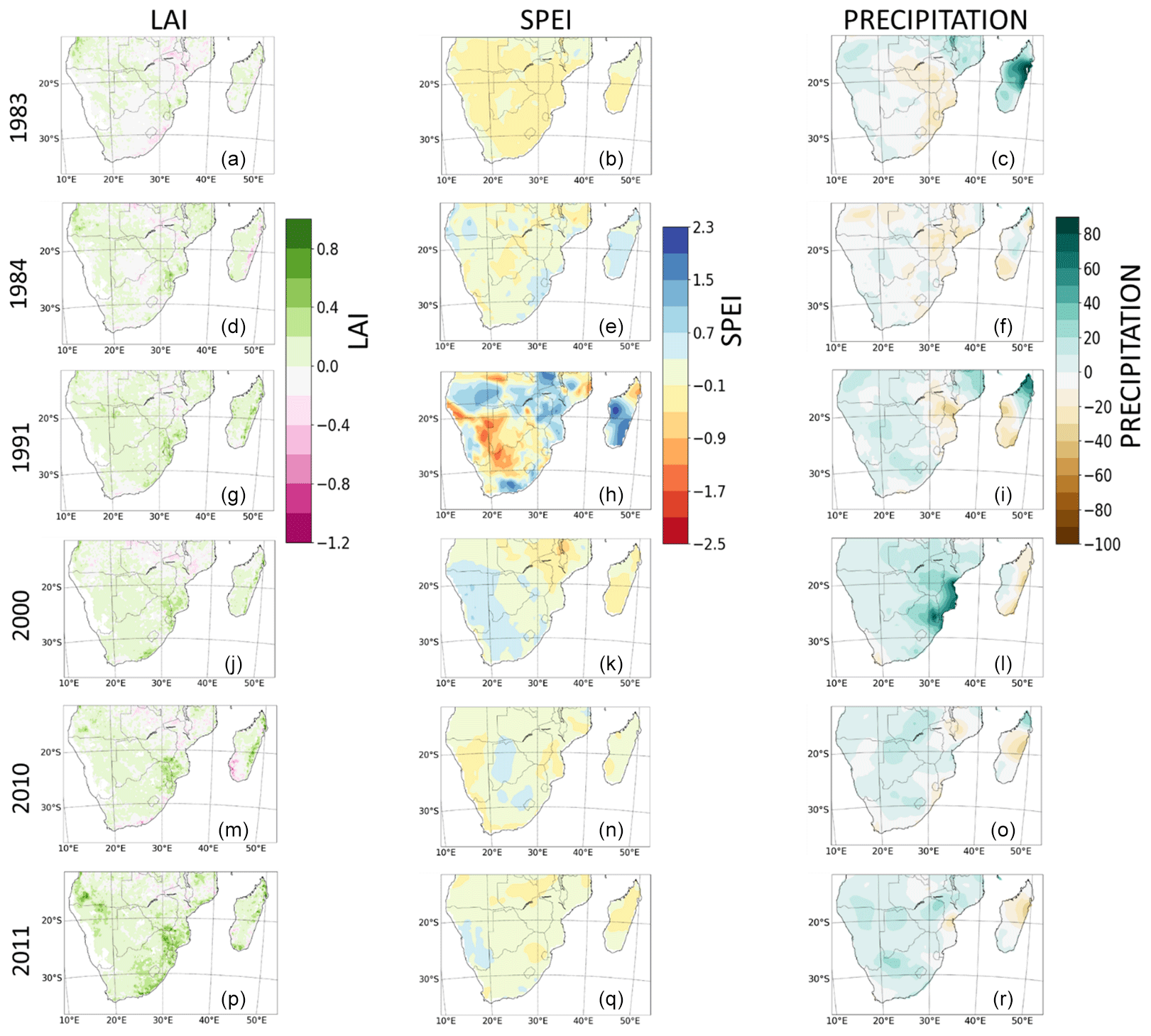
Figure 10Spatial pattern changes in satellite-calculated LAI, observed SPEI, and precipitation during extremely dry (1983, 1984, and 1991) and wet (2000, 2010, and 2011) years. For panels (a–i), the changes in LAI, SPEI, and precipitation were calculated as a difference between the dry year and the 30-year mean. For panels (j–r), changes in LAI, SPEI, and precipitation were calculated as the difference between the wet year and the 30-year mean. White areas indicate no correlation. The pattern correlation coefficients and the statistical significance of the coefficients between the variables are given in Table 5.
Note that, although the SPEI is a drought index, it was also considered in a wet year because the impact of drought usually lasts beyond a dry year, especially in semi-arid regions of southern Africa. In addition, the hot temperature has an influence on the worsening of the drought by causing water to evaporate from the soil. SPEI, as a drought index, considers temperature effects on moisture availability.
We considered only observation, i.e. CRU (precipitation and drought) and satellite-calculated LAI. The observed climate (CRU) data are not sub-monthly. Only the CRUJRA (reanalysis), which was used for model correlation, is sub-monthly. The model was not analysed in this section because our goal was simply to examine the observed impacts (or influence) of an extreme event.
The spatial pattern of change of LAI and SPEI are mostly similar during extreme dry and wet years (Fig. 10). For example, in 1983 (a dry year), the negative anomaly of LAI in some parts of the region largely follows the negative anomaly of the SPEI, except in the western and central parts (Fig. 10a and b). In 1984, both variables show a strong positive anomaly over Madagascar, Eswatini, and the KwaZulu-Natal province of South Africa (Fig. 10d and e). The pattern of change of both SPEI and LAI are also comparable during the extremely wet year. In the wet year of 2000, the positive anomaly of SPEI that is observed in Namibia and South Africa is also evident for the LAI (Fig. 10j and k). In a like manner, both variables show a negative anomaly over Malawi and Zambia. The strongest pattern (magnitudes) of change of the SPEI in the region is observed in the dry year of 1991 (Fig. 10h). However, the pattern of change of the LAI and SPEI are not similar over some regions in some periods. For instance, in 1991, while a negative anomaly of the SPEI is observed in northern Madagascar and central parts of southern Africa, LAI shows a positive anomaly (Fig. 10g and h). The opposite and decreasing relationship between the two variables in 1991 is also evident in the pattern correlation coefficient value of −0.16 (Fig. 10h). The variation in anomaly in these parts and period may be due to the exertion of a stronger influence by other factors such as residual soil moisture and precipitation (see Fig. 10i), with temperature having negligible impacts.
The influence of precipitation (as a standalone meteorological factor) on LAI during extreme events is limited. This is observed from the disparity in the spatial pattern of the LAI and precipitation over some regions and periods. For example, in 1984, the wide negative anomaly of precipitation that is shown over Zimbabwe, Mozambique, and southern Madagascar is opposite to the LAI, which shows positive anomaly (Fig. 10d and f). The LAI anomaly is more similar to that of the SPEI (Fig. 10e). Also, in wet year of 2000, while precipitation shows a preponderant increase over the northeastern parts of southern Africa, there is a decrease in the LAI, as is the case with SPEI (Fig. 10j–l). Nevertheless, precipitation plays a primary/major role in the pattern of change of LAI, as is observed over the most parts of the region during the years considered.
Generally, the pattern correlation coefficient values between the LAI and SPEI are higher than those between the LAI and precipitation in extremely dry and wet years (Table 5). Although the coefficients are small, they are mostly significant across the different extreme periods, except for 1983, an extremely dry year, where the p value is 0.58 for LAI–SPEI (Table 5). The extremely low statistical significance indicate low standard errors and a large number of grid sizes for the region.
Table 5Pattern correlation coefficients (r values) and significance of the coefficients calculated at a significance level of 5 % (α=0.05) between the LAI and SPEI for extremely dry and wet years, as well as between the LAI and precipitation during extremely dry and wet years. The correlation coefficients are significant when the p value is less than 0.05.
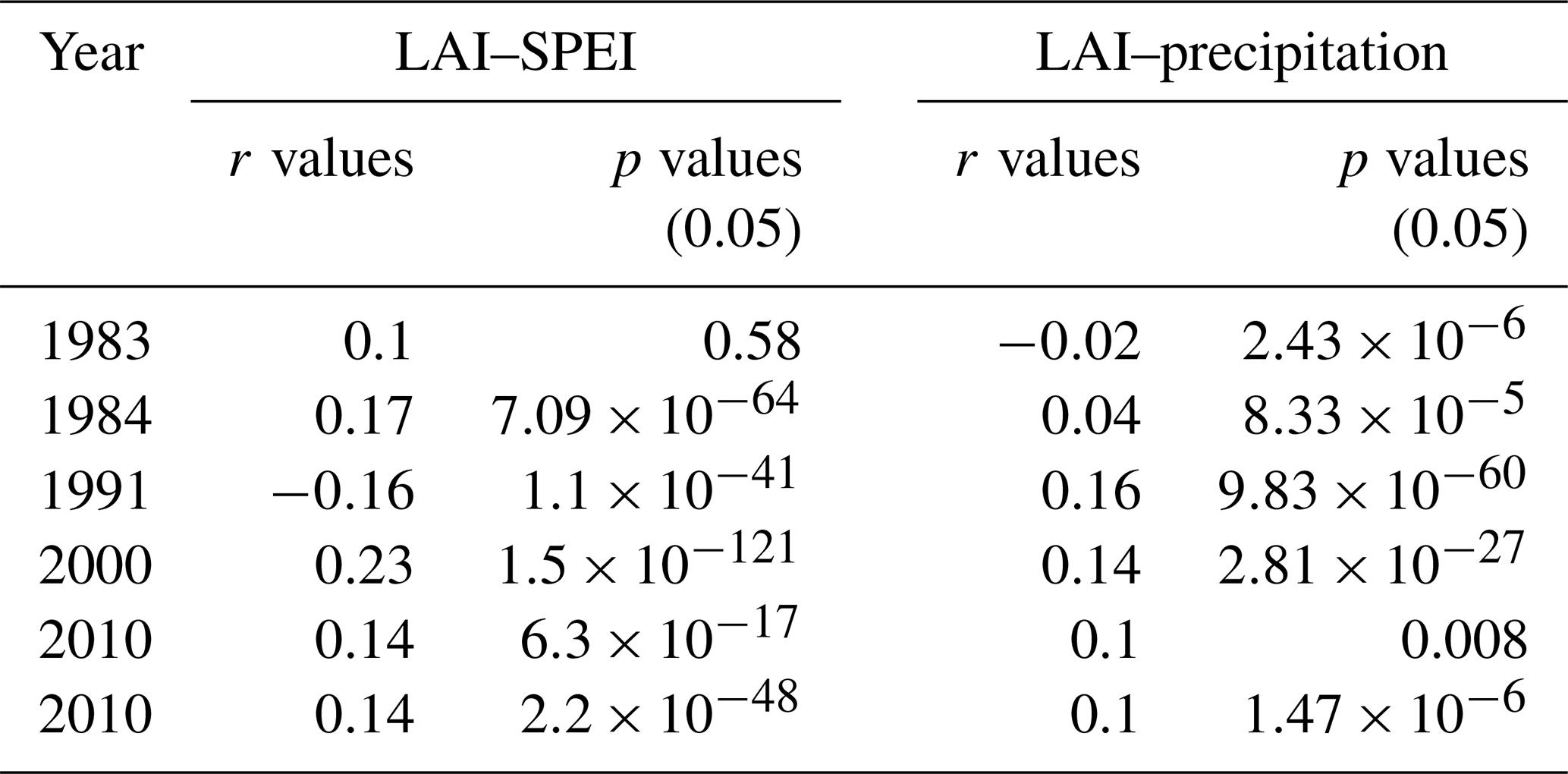
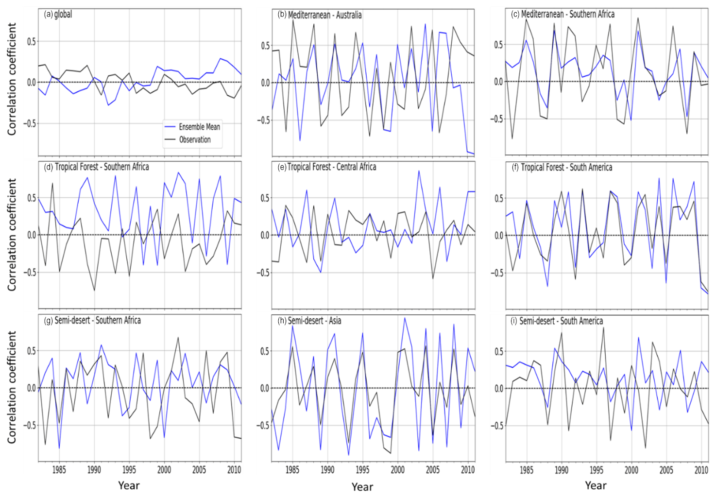
Figure 11Correlations between SPEI (12-month timescale) and the ensemble mean of LAI from TRENDY (blue line) and GIMMS LAI (black line) for (a) global vegetation, (b) Mediterranean vegetation over Australia, (c) Mediterranean vegetation over southern Africa, (d) a tropical forest over southern Africa, (e) a tropical forest over central Africa, (f) a tropical forest over South America, (g) a semi-desert biome over southern Africa, (h) a semi-desert over Asia, and (i) a semi-desert over South America.
3.10 Comparison of global and regional distribution of LAI response to droughts (1982–2011)
There is variability in the global and regional temporal distribution of the LAI response to drought (at a 12-month timescale) when global vegetation biomes are split into regional biomes (Fig. 11). The map of the global biomes is shown in Fig. S1 in the Supplement. The observed global response indicates a decreasing trend of the LAI response to drought, while the model mean shows an increasing estimate.
The semi-desert biome dominates the LAI response as higher drought–vegetation correlations are observed (Fig. 11g–i). Over the biome, there is a more marked interannual variability, which makes the biome an important player in the global carbon cycling (Poulter et al., 2014). The response over the semi-desert in southern Africa is, however, weaker in comparison to the other semi-desert biomes.
The response over the Mediterranean vegetation in Australia is stronger than the Mediterranean vegetation over the rest of inland southern Africa. Over the biome, the model simulates closer magnitudes in the latter than over Australia (Figs. 11b and 9c).
Over the tropical forest biomes, there is a weaker response in central Africa compared to southern Africa and South America; the model simulates the closest response in magnitude in South America (Fig. 11d and f).
4.1 Relationship of LAI to phenological changes
LAI is a variable that is needed for the global modelling of biogeochemistry, climate, ecology and hydrology, and different primary production models (e.g. Running and Coughlan, 1988; Sellers et al., 1996; Bonan et al., 2002). In view of the need to run biogeochemical models at regional and global scales, accurate LAI data at moderate to high resolutions are crucial (Wang et al., 2004). The relationship between NDVI and LAI is applied as a support algorithm in MODIS LAI. Thus, from the viewpoint of the availability of data, retrieving LAI from analysing the NDVI–LAI relationship remains the main perspective for high temporal resolution in regional and global studies (Wang et al., 2004).
LAI showed a linear relationship with NDVI. This suggests that the NDVI is associated with the phenological changes in plants, the parts of the surface cover class which contribute to the general reflectance, and the variations in the angle of solar zenith (Wang et al., 2004). Studies (e.g. Myoung et al., 2013) have, however, found that the relationship between NDVI and LAI varies intra- and interannually, and both vegetation indices differ temporally and seasonally over deciduous forests, which are sometimes not accounted for in models that test their relationship (Wang et al., 2004). For instance, while the relationship is strong during periods of leaf production and senescence, no relationship is observed during the period of leaf constant due to NDVI saturation above certain LAI values (Xue and Su, 2017).
Although the present study found a strong linear relationship between the NDVI and LAI in southern Africa, other studies (Potithep et al., 2010; Towers et al., 2019) have shown that the two indices are not always directly proportional. For example, both indices do not exhibit the same relationships over different ecoregions such as the evergreen broadleaf forest or deciduous needleleaf forest. Furthermore, other studies (Fan et al., 2008; Tian et al., 2017) found that the LAI may be a better indicator of plant biomass and health because of the saturation associated with the NDVI, particularly in the drylands. This makes the LAI more applicable in monitoring the vegetation response to drought. Evaluating how the LAI differs from the NDVI over different biomes (such as dry savanna, tropical forest, etc.), with regards to temporal difference, is shown in Fig. S7. Both the LAI and NDVI show similar annual cycles over southern Africa, except for the tropical forest and Mediterranean vegetation.
4.2 The importance of sub-monthly data in drought computation and monitoring
The data used to evaluate drought indices are CRUJRA. JRA is a reanalysis data set and has a 6 h temporal resolution. Additionally, CRUJRA have the data used to force the DGVMs, so the drought indices are being calculated based on the same data the models use for their simulations. JRA is a reanalysis data set, but the combined CRUJRA product uses the sub-monthly information from JRA and is constrained to the monthly CRU observations. The comparisons of the data are shown in Figs. 5 and S6. It is useful to use data with shorter times because the study focuses on an evaluation of drought impact, which is sensitive to the timescale. In the drylands, for instance, the uncertainties associated with monthly data in drought monitoring are reduced when sub-monthly data are used (Mukherjee et al., 20117). With regards to the precipitation and temperature fields, the difference is negligible.
We note that, over different parts of the world, CRU has been widely validated against station data (Harris et al., 2020), and there is a high accuracy of the validation. Therefore, observed SPEI gives a high accuracy of measured drought. Another major advantage of using the observational-based CRU data is its spatial and temporal coverage. Station data are available for very few points and for limited times in the region of interest. The few data that are available are fraught with missing data, rendering them an unreliable data source (Harris et al., 2020).
4.3 Annual cycle of climate and vegetation in southern Africa
Climatologies of meteorological variables show that precipitation drops in JJA and SON seasons over the biomes, except over the Mediterranean vegetation. The dry condition that is experienced during these seasons could be attributed to the subtropical high pressure system which suppresses rainfall by shifting the ITCZ (Intertropical Convergence Zone) away from these regions (Naik and Abiodun, 2016).
Observations also show low LAI over some parts of southern Africa (please see Fig. S2). The weak gradient in some parts of the region may be due to low winter rains produced by the frontal system, which is not sufficient for growth of expanse vegetation (Lange et al., 1999). The aridification of the western part of southern Africa may be attributed to the influence of cold sea surface temperatures (SSTs) of the Namibian upwelling system along the Namibian coasts (Ward et al., 1983). The aridification does not only result in the cessation of river discharge but also sediments that would have favoured the growth of drier vegetation (Dupont, 2006).
For Fig. S5, some of the models do not capture this peak around September over the Mediterranean and tropical biomes. One possible explanation is that the models do not reproduce the changes in the biomass and leaf area cover around that period well (due to phenological responses to environmental variables). For both biomes, spring rainfall contributes to vegetation growth in the region, which may not be reproduced well by the models. For Fig. 4, the magnitudes (<0.5) of the observation-based LAI over (southern Africa) semi-desert biome is quite high because the region is a pseudo-desert, which experiences very high summer temperatures but does receives some rainfall, and the Okavango River is flowing through it permanently. This region is rich in biodiversity such as Acacia spp. (trees) and Aristida and Schmidtia spp. (savanna; see WWF, 2001; Street and Prinsloo, 2013; Lawal, 2018) Thus, a 0.5 LAI in the biome, which may be higher than other desert biomes, is reasonable in this region.
4.4 LAI response to drought in observation
Drought is becoming frequent and more intense in southern Africa (Masih et al., 2014). The frequent and stronger dry spells are observed in Fig. 6. Climate change is expected to increase the frequency and severity of droughts (Tables 2 and 3). The severity and longer durations of drought have enormous impacts on the already endangered vegetation biomes in the region (Hoffman et al., 2009). The results show that drought impacts on vegetation occur across the different seasons in the region. The seasonal difference in the response of vegetation to drought across biomes is influenced by numerous factors, such as vegetation adaptive capacity and resilience, reproduction process, and growth stage, among others (Zeppel et al., 2014; Corlett, 2016). For instance, over the tropical forest biome, drought has the least impact on vegetation in the region, which could be because of the deeper rooting system of the vegetation which allows access to soil at the deeper water table (El-Vilaly et al., 2017). It is reported that major drivers of vegetation resilience and productivity are precipitation and temperature which control the evapotranspiration rate (Allen et al., 2010). It is worth noting that vegetation in southern Africa will be severely impacted if the trends continue in the same trajectory. For instance, the regions where there is a strong vegetation response to drought are experiencing wood encroachment and, thus, will likely worsen based on the current trajectory of drought occurrence.
We note that the performance of drought indices is not only limited by the variables used in their computation but also by biomes and locations where they are used (Xu et al., 2015). For example, SPI, which is calculated using simple methods and has adaptable timescales, performs better than SPEI in arid regions (Beguería et al., 2014). However, SPEI, which requires more variables for its computation, captures drought better in relatively humid zones (Beguería et al., 2014). SPEI is, however, limited by the potential evapotranspiration (PET) because of its sensitivity to the variable (Xu et al., 2015).
The vegetation situated at the borders of Botswana–Namibia and Mozambique–Zambia respond to droughts at an intermediate timescale (i.e. 9 months). The types of vegetation inhabiting these regions, which are well adapted to water shortages because of their physiological and morphological characteristics, take a prolonged period to respond to drought and, thus, do not easily shows symptoms of water strain (Vicente-Serrano, 2013). The activities through which the vegetation minimize water loss include a reduction in photosynthesis and reduced canopy cover (Schwinning et al., 2005). The capacity for vegetation to store water is one adaptation for low water ecosystems, as is reduced daytime stomatal conductance and crassulacean acid metabolism (CAM) photosynthesis. The disparity in the timescale's spatial distribution in models from observation might be because the parameters are represented and estimated in the models (Murray et al., 2011). In addition, the models are not similar in their drought timescale simulations.
The varying response of the tropical forests in different regions may be because of the interplay of precipitation and temperature at different longitudes. Ahlström et al. (2015) showed that temperature is a particularly a strong factor in the response of this vegetation. Wang et al. (2008) also reported that soil moisture variations play a key role in the magnitude of vegetation response. The weak response of LAI to drought over Madagascar and Angola may be attributed to the fact that the vegetation in these regions is able to store water for a long time which it uses during deficit periods (Chapotin et al., 2006). It may also be because rainfall is not the main regulatory component in the growth of vegetation in these regions (Fuller and Prince, 1996). In regions such as Botswana and Namibia, the vegetation is highly dependent on water availability for its ecosystem functions (Anyamba et al., 2003). Please see Fig. S3 for the observed correlations at different timescales.
The seasonal response of LAI to drought varies, and this could be attributed to many factors. For instance, the sensitivity of the semi-desert to water shortage makes them show a quick response to drought (New, 2015). The response of vegetation to drought is particularly stronger in the MAM season because it is during this period that fruit, leaves, and biomass are produced by vegetation (Zeppel et al., 2014). The critical water requirement by vegetation for these developmental activities in the MAM season is the reason for the vegetation's response to droughts at a short timescale (Zeppel et al., 2014). The strongest vegetation response (a correlation of about 0.92) is observed over the semi-desert biome (which is in the semi-arid environment) in the JJA season. This is a region with vegetation which is heavily dependent on water for all the ecosystems' functioning and without which they would not survive (New, 2015). The drought response of the tropical forest is weaker compared to all other biomes. Over the tropical forest biome, the fairly subtle drought response may be because the biome can be tolerant to drought, have a stronger, robust capacity, and is, therefore, not extremely impacted by droughts as the other biomes are (Gielen et al., 2005; Corlett, 2016).
The different responses by the global biomes in different geographical locations may be because of climate variations and the sensitivity of LAI to climate variations (Ahlström et al., 2015). The dominance of the LAI response to drought over the semi-desert biome could be attributed to the global bush encroachment and is in consonance with the increasing greenness (Donohue et al., 2009; Fensholt et al., 2012; Andela et al., 2013). Studies (Cai et al., 2014; Trenberth et al., 2014; Dai, 2013; Wang et al., 2014; Ahlström et al., 2015) have also found that increased and frequent El Niño–Southern Oscillation (ENSO) events due to climate change have not only led to the expansion of LAI but could increase the water demand by semi-desert vegetation. This comparison is particularly important because, until now, there has been little or no study on this.
4.5 How well the seasonal and interannual variations of LAI are captured in DGVM simulations
The models exhibit biases in the simulation of seasonal and interannual variations of LAI over southern Africa. There are two major factors that may be given for the performance of the models. First, the influence of precipitation forcing data largely affect the seasonal cycle of LAI and the interannual variability (see Figs. 3 and S8). Although the difference between the forcing data for observed and modelled LAI (i.e. CRU and CRUJRA, respectively) is small, it still influences the simulations by the DGVMs. The precipitation uncertainty has a larger influence in some regions and biomes than others. For instance, the overestimation of LAI by models in the arid biome of Namibia and the Mediterranean vegetation of South Africa may be due to the irregularity in precipitation, whereby the precipitation changes are too small to be identified (in CRUJRA), and due the large spatial variability (Fekete et al., 2004; Greve et al., 2014). On the other hand, over the savanna biome of Angola, the underestimation is likely because of the sparse distribution of precipitation data, which permeates to CRUJRA (Fekete et al., 2004). Second, the differences in observed and simulated LAI may be due to the impacts of land use and land cover change (LULCC) on the latter in the simulation through soil moisture and evapotranspiration (Piao et al., 2007). LULCC exerts a strong influence on water consumption, nutrient cycling, and root depth (Piao et al., 2007; Mango et al., 2011), and the extent of the influence also varies across biomes. For example, in MAM, over the temperate grassland biome of South Africa, where the model underestimates LAI, the bias is likely because the models fail to simulate the frequency of evapotranspiration, which is about 5 times less than the forest biome (Yang et al., 2015).
However, over most parts of the region, the correlation between observed and modelled LAI is strong, except in the JJA season. This means that the models generally simulate the pattern of LAI distribution in southern Africa. We also note that the lower correlations between observed and modelled LAI, when the data were deseasonalized, is due to the sensitivity of LAI to variability and seasonality. These differences between the observed and modelled system have impacts on how the vegetation response to drought is captured, which we discuss in Sect. 4.6.
4.6 How well drought and LAI response is represented in DGVM simulations
The observed LAI is simulated within the models and calculated by GIMMS, based on Mao and Yan (2019). Lu et al. (2011) found that DGVMs perform better against observations than Earth system models (ESMs) because they use observational-derived climate and can include more complex representations of vegetation processes. The ESM is a coupled model simulating its own climate, while the individual DGVMs models used in the present study are standalone models, i.e. are applied with observational-based meteorological forcing, and thus, we remove one uncertainty. Since offline studies target the DGVM itself, removing one possible issue (incorrect climate drivers), it became imperative to use DGVM to study drought impacts.
DGVMs simulate the vegetation characteristics and impacts of climate on them. The validation of DGVM simulations of variables such as LAI is quite difficult. This is because of the unavailability of data on a large spatiotemporal scale for the different vegetation classes (Potter and Klooster, 1998). Studies (e.g. Potter and Klooster, 1998) have also shown that errors present in the prediction of plant functional types (PFTs) tend to spread to biomass prediction in the model, thus possibly biassing estimates of carbon stored in terrestrial ecosystems. Nevertheless, the DGVMs used in this study simulate the spatial patterns of vegetation distribution with a magnitude bias, as shown in Fig. S2.
TRENDY models mostly simulate the temporal patterns in the global and regional distributions of LAI response to drought. The biases shown by the models have been attributed to the fact that the models do not factor in land use changes (Ahlström et al., 2015). This is evident in the simulation of LAI (please see Fig. S2).
The model's weaker simulations might also be because some of the DGVMs do not reproduce the LAI magnitude well. The negligible difference in the spatial distributions of the SPEI of the models could be due to fact that the model PET does not play a strong role in drought occurring in southern Africa and that precipitation is the main driver of drought in the region. The variations in the characterization of hydrological processes in the models are also a source of uncertainty because they reinforce the bifurcation in runoff outputs, which has cascading effects on biospheric changes and evapotranspiration (Murray et al., 2011; Stewart et al., 2004). Also see Fig. S4 for the correlations of the model ensemble median at different timescales. Another reason for the biases in the simulations may due be to the design of the DGVM experimental set up, which includes the flux deviation between simulations (Murray et al., 2011).
4.7 Variations in observed and simulated vegetation response to drought and implications on model development
The biases shown by models could be attributed to the different limitations of individual DGVMs, and addressing these shortcomings would improve the model's performance. For example, the sub-optimal performance of CLM may be partly due to the inability of the model to capture the foliage production and root system of vegetation for transpiration. The model is also unable to produce savanna ecosystems, which it simulates by approximating the vegetation of forest and grassland ecoregions (Dahlin et al., 2020). In addition, the ineffective simulation of deciduousness would have contributed to the model biases in response simulations. Therefore, targeting these limitations is important for improving the model's performance in simulating morphology and physiological functioning of vegetation biomes. Furthermore, the DGVMs (e.g. JULES and DLEM) used in the study poorly replicate important ecological and physiological processes that are critical for capturing the dynamics of savanna systems. Other DGVMs (e.g. JSBACH) poorly simulate significant environmental variables such as fire, which is very crucial for the vegetation growth cycle, particularly in the savanna biome (Thonicke et al., 2001; Romps et al., 2014; Kim et al., 2018; D'Onofrio et al., 2020). Also, over southern Africa, land use change (LUC) is a common and frequent occurrence and is an important factor for vegetation turnover. However, most models do not capture land management well, which is an important driver of land cover change in the region. Thus, there is a need for future model development to account for rapid LUC over different regions. However, the disparity in the observed and simulated response of vegetation to drought cannot be fully accounted by the DGVMs alone. The reanalysis (CRUJRA) has also shown some limitations in the simulation of climate variables. Compared to observation-based CRU, CRUJRA has closer magnitudes of maximum and minimum temperature, and addressing this would improve the simulated response.
Southern African vegetation is continually affected by drought. In this study, we estimated the spatiotemporal characteristics of meteorological drought in southern Africa using the Standardized Precipitation Evapotranspiration Index (SPEI) over a 30-year period (1982–2011). The severity of the drought and its impacts on vegetation production were examined at various drought timescales (1- to 24-month timescales) by correlating the drought index (SPEI) with GIMMS LAI at different timescales. We found that the LAI responds strongly (r=0.6) to drought over the central and southeastern parts of the region, with weaker impacts (r<0.4) over parts of Madagascar and Angola, mostly at a shorter time period (3- and 6-month timescale). We note that comparing CRU to flux tower precipitation in Skukuza (KwaZulu-Natal region) illustrates that CRU captures the timing of precipitation relatively well, though it underestimates the magnitude of dry season precipitation (Fig. S9). For seasonal responses, the semi-desert biome showed the strongest response (r=0.95) to drought at a 6-month timescale in the autumn season, while the tropical forest biome shows the weakest response (r=0.35) at a 6-month timescale in the DJF season.
We assessed the relationship between the NDVI and LAI by computing a grid cell correlation of NDVI and LAI and examined how well state-of-the-art dynamic global vegetation models (DGVMs) simulate LAI and its response to drought. The DGVM multimodel ensemble mostly overestimated the spatial and seasonal distribution of LAI response to drought in most parts of the region. The results also show the following:
-
The relationship between the NDVI and LAI is linear, implying that the vegetation index is connected to the changes in the phenology of the plant, reflectance, and the angle of zenith variations from the surface cover class.
-
The model ensemble simulates the correlation and timescale of LAI response to drought with biases.
-
The model ensemble overestimates observed responses on the seasonal distribution of vegetation–drought correlations across different biomes.
-
The spatial pattern of change of the LAI and SPEI are mostly similar during extremely dry and wet years, with the highest magnitudes of anomaly observed in the dry year of 1991. During this period, both variables also show an opposite and decreasing relationship, which is evident in their pattern correlation coefficient value of −0.16.
The present study has shown how the LAI responds to drought across the different southern African biomes. Given the present spatial coverage of space monitoring of the vegetation in the region, the methods used in the study may be extended towards monitoring and characterizing the impacts of droughts on land cover change, as this may permit real-time monitoring of extreme events on terrestrial vegetation (Yin et al., 2020; Moore et al., 2018). The findings of this study (e.g. timescales of the LAI response to drought) could also be used for the development of drought early warning systems in agriculture and forestry sectors. This could assist in the mitigation of direct and indirect costs associated with vegetation production.
Furthermore, this study has applied 11 DGVMs to study how well DGVMs can reproduce the response of LAI in southern African vegetation to drought. While this study may have provided an insight into the capability of DGVMs to simulate vegetation response to drought, the results of the study can, however, be improved in some ways. For example, we applied 11 models from the TRENDY DGVMs. For future studies, the number of models should be increased, perhaps from other model intercomparison experiments, because, by using more models and better quantification, this might capture uncertainty better in their simulation of the drought response by vegetation. The limitation of the DGVMs can be addressed by optimizing the models so that their capability for reproducing vegetation indices is enhanced and better quantified. In addition, there is a need to improve the mechanistic relationships in the models, which could be achieved by enhancing the model approximations, which had been done to achieve computational efficiencies (Transtrum and Qiu, 2016). Furthermore, the simple phenomenological model could be developed from the complex model. These simple models would use correlations among observations, unlike mechanistic relationships, which exploit causative individual constituent and suffer from over-fitting problems (Transtrum and Qiu, 2016). Last, there may be the need for hybridizing machine learning and mechanistic models (Fayyad et al., 1996; Mitchell, 1997) to simulate vegetation parameters. This is because machine learning models have shown a certain advantage in the prediction of outcomes of complex mechanisms by using databases of inputs and outputs for a given task (Fayyad et al., 1996; Mitchell, 1997).
The sources of data used in this work are provided in Sect. 2.1 and comprise the CRU (Mitchell and Jones, 2005; Harris et al., 2014), CRUJRA (University of East Anglia Climatic Research Unit; Harris et al., 2020), NDVI3g (Mao and Yan, 2019), and Trendy DGVMS (Sitch et al., 2008; Clark et al; 2011; Zaehle et al., 2011; Kato et al., 2013; Oleson et al., 2013; Le Quéré et al., 2014; Joetzjer et al., 2015; Melton and Arora, 2016; Goll et al., 2017; Haverd et al., 2018; Tian et al., 2015; Mauritsen et al., 2018; Lienert and Joos, 2018).
The supplement related to this article is available online at: https://doi.org/10.5194/hess-26-2045-2022-supplement.
SL was responsible for conceptualization, developing the initial content of the paper, including the literature search, data analysis, and writing of the paper. SS and DL provided model outputs and guided on data analysis. JN, HWW, PF, HT, and BH provided the model output and guidance in terms of the article structure and finalization of the paper.
The contact author has declared that neither they nor their co-authors have any competing interests.
Publisher's note: Copernicus Publications remains neutral with regard to jurisdictional claims in published maps and institutional affiliations.
The work has been supported by the South African National Research Foundation (NRF).
This paper was edited by Shraddhanand Shukla and reviewed by two anonymous referees.
Allen, C. D., Macalady, A. K., Chenchouni, H., Bachelet, D., McDowell, N., Vennetier, M., and Gonzalez, P.: A global overview of drought and heat-induced tree mortality reveals emerging climate change risks for forests, Forest Ecol. Manage., 259, 660–684, https://doi.org/10.1016/j.foreco.2009.09.001, 2010.
Ahlström, A., Raupach, M. R., Schurgers, G., Smith, B., Arneth, A., Jung, M., Reichstein, M., Canadell, J. G., Friedlingstein, P., Jain, A. K., Kato, E., Poulter, B., Sitch, S., Stocker, B. D., Viovy, N., Wang, Y. P., Wiltshire, A., Zaehle, S., and Zeng, N.: The dominant role of semi-arid ecosystems in the trend and variability of the land CO2 sink, Science, 348, 895–899, https://doi.org/10.1126/science.aaa1668, 2015.
Andela, N., Liu, Y. Y., van Dijk, A. I. J. M., de Jeu, R. A. M., and McVicar, T. R.: Global changes in dryland vegetation dynamics (1988–2008) assessed by satellite remote sensing: Comparing a new passive microwave vegetation density record with reflective greenness data, Biogeosciences, 10, 6657–6676, https://doi.org/10.5194/bg-10-6657-2013, 2013.
Anyamba, A., Justice, C. O., Tucker, C. J., and Mahoney, R.: Seasonal to interannual variability of Vegetation and fires at SAFARI 2000 sites inferred from advanced very high resolution Radiometer time series data, J. Geophys. Res., 10, 8507, https://doi.org/10.1029/2002JD002464, 2003.
Beguería, S., Vicente-Serrano, S. M., Reig, F., and Latorre, B.: Standardized precipitation evapotranspiration index (SPEI) revisited: parameter fitting, evapotranspiration models, tools, datasets and drought monitoring, Int. J. Climatol., 34, 3001–3023, https://doi.org/10.1002/joc.3887, 2014.
Bonan, G. B., Oleson, K. W., Vertenstein, M., Lewis, S., Zeng, X., Dai, Y., Dickinson, D. E., and Yang, Z.: The land surface climatology of the NCAR land surface model coupled to the NCAR community climate model, J. Climate, 11, 1307–1327, 2002.
Cai, W., Borlace, S., Lengaigne, M., van Rensch, P., Collins, M., Vecchi, G., Timmermann, A., Santoso, A., McPhaden, M. J., Wu, M., England, L. H., Wang, G., Guilyardi, E., and Jin, F.-F: Increasing frequency of extreme El Nino events due to greenhouse warming, Nat. Clim. Change, 4, 111–116, https://doi.org/10.1038/nclimate2100, 2014.
Chapotin, S. M., Razanameharizaka, J. H., and Holbrook, N. M.: Water relations of baobab trees (Adansonia spp L.) during the rainy season. Does stem water buffer daily water deficit, Plant Cell Enviro., 29, 1021–1032, 2006.
Clark, D. B., Mercado, L. M., Sitch, S., Jones, C. D., Gedney, N., Best, M. J., Pryor, M., Rooney, G. G., Essery, R. L. H., Blyth, E., Boucher, O., Harding, R. J., Huntingford, C., and Cox, P. M.: The Joint UK Land Environment Simulator (JULES), model description – Part 2: Carbon fluxes and vegetation dynamics, Geosci. Model Dev., 4, 701–722, https://doi.org/10.5194/gmd-4-701-2011, 2011.
Corlett, R. T.: The Impacts of Droughts in Tropical Forests, Trends Plant Sci., 21, 584–593, https://doi.org/10.1016/j.tplants.2016.02.003, 2016.
Dahlin, K. M., Fisher, R. A., and Lawrence, P. J.: Environmental drivers of drought deciduous phenology in the Community Land Model, Biogeosciences, 12, 5061–5074, https://doi.org/10.5194/bg-12-5061-2015, 2015.
Dahlin, K. M., Akanga, D., Lombardozzi, D. L., Reed, D. E., Shirkey, G., Lei, C., Abraha, M., and Chen, J.: Challenging a global land surface model in a local socio-environmental system, Land, 9, 1–21, https://doi.org/10.3390/land9100398, 2020.
Dai, A.: Increasing drought under global warming in observations and models, Nat. Clim. Change, 3, 52–58, https://doi.org/10.1038/nclimate1633, 2013.
DEA – Department of Environmental Affairs: Climate Change Adaptation Plans for South African Biomes, edited by: Kharika, J. R. M., Mkhize, N. C. S., Munyai, T., Khavhagali, V. P., Davis, C., Dziba, D., Scholes, R., van Garderen, E., von Maltitz, G., Le Maitre, D., Archibald, S., Lotter, D., van Deventer, H., Midgely, G., and Hoffman, T., DEA, Pretoria, 2015.
D'Onofrio, D., Baudena, M., Lasslop, G., Nieradzik, L. P., Wårlind, D., and von Hardenberg, J.: Linking vegetation-climate-fire relationships in subsaharan africa to key ecological processes in two dynamic global vegetation models, Front. Environ. Sci., 8, 136, https://doi.org/10.3389/fenvs.2020.00136, 2020.
Donohue, R. J., McVicar, T. R., and Roderick, M. L.: Climate-related trends in Australian vegetation cover as inferred from satellite observations, 1981–2006, Global Change Biol., 15, 1025–1039, https://doi.org/10.1111/j.1365-2486.2008.01746.x, 2009.
Driver, A., Sink, K. J., Nel, J. N., Holness, S., Van Niekerk, L., Daniels, F., Jonas, Z., Majiedt, P. A., Harris, L., and Maze, K.: National Biodiversity Assessment 2011: An assessment of South Africa's biodiversity and ecosystems, Synthesis Report, South African National Biodiversity Institute and Department of Environmental Affairs, Pretoria, 2012.
Dupont, L. M.: Late Pliocene vegetation and Climate and Namibia (Southern Africa) derived From Palynology of ODP site 1082, Geochem. Geophy. Geosy., 7, Q05007, https://doi.org/10.1029/2005GC001208, 2006.
El-Vilaly, M. A. S., Didan, K., Marsh, S. E., van Leeuwen, W. J., Crimmins, M. A., and Munoz, A. B.: Vegetation productivity responses to drought on tribal lands in the four corners region of the Southwest USA, Front. Earth Sci., 12, 37–51, https://doi.org/10.1007/s11707-017-0646-z, 2017.
Fan, L., Gao, Y., Brück, H., and Bernhofer, C.: Investigating the relationship between NDVI and LAI in semi-arid grassland in Inner Mongolia using in-situ measurements, Theor. Appl. Climatol., 95, 151–156, https://doi.org/10.1007/s00704-007-0369-2, 2008.
Fan, L., Wigneron, J. P., Ciais, P., Chave, J., Brandt, M., Fensholt, R., Saatchi, S. S., Bastos, A., Al-Yaari, A., Hufkens, K., Qin, Y., Xiao, X., Chen, C., Myneni, R. B., Fernandez-Moran, R., Mialon, A., Rodriguez-Fernandez, N. J., Kerr, Y., Tian, F., and Peñuelas, J.: Satellite observed pantropical carbon dynamics, Nat. Plants, 5, 944–951, 2019.
FAO: FAO/ESAF Handbook for Defining and Setting up a Food Security Information and Early Warning System (FSIEWS), FAO, Rome, 2000b.
Fayyad, U., Piatetsky-Shapiro, G., and Smyth, P. (Eds): From data mining to knowledge discovery Databases, AI Magazine, 17, 37, 1996.
Fekete, B. M., Vörösmarty, C. J.,Roads, J. O., and Willmott, C. J.: Uncertainties in precipitation and their impacts on runoff estimates, J. Climate, 17, 294–304, https://doi.org/10.1175/1520-0442(2004)017<0294:UIPATI>2.0.CO;2, 2004.
Fensholt, R., Langanke, T., Rasmussen, K., Reenberg, A., Prince, S. D., Tucker, C., Scholes, R. J., Le, Q. B., Bondeau, A., Eastman, R., Epstein, H., Gaughan, A. E., Hellden, U., Mbow, C., Olsson, L., Paruelo, J., Schweitzer, C., Seaquist, J., and Wessels, K.: Greenness in semi-arid areas across the globe 1981–2007 – an Earth Observing Satellite based analysis of trends and drivers, Remote Sens. Environ., 121, 144–158, https://doi.org/10.1016/j.rse.2012.01.017, 2012.
Forkel, M., Carvalhais, N., Verbesselt, J., Mahecha, M. D., Neigh, C. S. R., and Reichstein, M.: Trend Change Detection in NDVI Time Series: Effects of Inter-Annual Variability and Methodology, Remote Sens., 5, 2113–2144, https://doi.org/10.3390/rs5052113: 2013.
Fuller, D. O. and Prince, S. D.: Rainfall and foliar dynamics in tropical southern Africa: Potential impacts of global climatic change on savanna vegetation, Climatic Change, 33, 69–96, https://doi.org/10.1007/BF00140514, 1996.
Gielen, B., De Boeck, H, Lemmens, C. M. H. M., Valcke, R., Nijs, I., and Ceulemans, R.: Grassland species will not necessarily benefit from future elevated air temperatures: a chlorophyll fluorescence approach to study autumn physiology, Physiol. Plant, 125, 52–63, https://doi.org/10.1111/j.1399-3054.2005.00539.x, 2005.
Gitelson, A. A.: Wide dynamic range vegetation index for remote quantification of biophysical characteristics of vegetation, J. Plant Physiol., 161, 165–173, https://doi.org/10.1078/0176-1617-01176, 2004.
Goll, D. S., Vuichard, N., Maignan, F., Jornet-Puig, A., Sardans, J., Violette, A., Peng, S., Sun, Y., Kvakic, M., Guimberteau, M., Guenet, B., Zaehle, S., Penuelas, J., Janssens, I., and Ciais, P.: A representation of the phosphorus cycle for ORCHIDEE, Geosci. Model Dev., 10, 3745–3770, https://doi.org/10.5194/gmd-10-3745-2017, 2017.
Greve, P., Orlowsky, B. Mueller, J. Sheffield, M. Reichstein, and Seneviratne, S. I.: Global assessment of trends in wetting and drying over land, Nat. Geosci., 7, 716–721, https://doi.org/10.1038/ngeo2247, 2014.
Hao, Z. and AghaKouchak, A.: Multivariate standardized drought index: a parametric multi-index model, Adv. Water Resour., 57, 12–18, https://doi.org/10.1016/j.advwatres.2013.03.009, 2013.
Harris, I., Jones, P. D., Osborn, T. J., and Lister, D. H.: Updated high-resolution grids of monthly climatic observations – the CRU TS3.10 Dataset, Int. J. Climatol., 34, 623–642, https://doi.org/10.1002/joc.3711, 2014.
Harris, I., Osborn, T. J., Jones, P., and Lister, D.: Version 4 of the CRU TS monthly high-resolution gridded multivariate climate dataset, Scient. Data, 7, 109, https://doi.org/10.1038/s41597-020-0453-3, 2020.
Haverd, V., Smith, B., Nieradzik, L., Briggs, P. R., Woodgate, W., Trudinger, C. M., Canadell, J. G., and Cuntz, M.: A new version of the CABLE land surface model (Subversion revision r4601) incorporating land use and land cover change, woody vegetation demography, and a novel optimisation-based approach to plant coordination of photosynthesis, Geosci. Model Dev., 11, 2995–3026, https://doi.org/10.5194/gmd-11-2995-2018, 2018.
Hoffman, M. T., Carrick, P. J., and West, A. G.: Drought, climate change and vegetation response in the succulent karoo, South Africa, S. Afr. J. Sci., 105, 61–68, https://doi.org/10.4102/sajs.v105i1/2.40, 2009.
Joetzjer, E., Delire, C., Douville, H., Ciais, P., Decharme, B., Carrer, D., Verbeeck, H., De Weirdt, M., and Bonal, D.: Improving the ISBACC land surface model simulation of water and carbon fluxes and stocks over the Amazon forest, Geosci. Model Dev., 8, 1709–1727, https://doi.org/10.5194/gmd-8-1709-2015, 2015.
Kato, E., Kinoshita, T., Ito, A., Kawamiya, M., and Yamagata, Y.: Evaluation of spatially explicit emission scenario of landuse change and biomass burning using a process-based biogeochemical model, J. Land Use Sci., 8, 104–122, https://doi.org/10.1080/1747423X.2011.628705, 2013.
Khosravi, H., Haydari, E., Shekoohizadegan, S., and Zareie, S.: Assessment the effect of drought on vegetation in desert area using landsat data Egypt, J. Remote Sens. Space Sci., 2007, S3–S12, https://doi.org/10.1016/j.ejrs.2016.11.007, 2017.
Kim, J. B., Kerns, B. K., Drapek, R. J., Pitts, G. S., and Halofsky, J. E.: Simulating vegetation response to climate change in the Blue Mountains with MC2 dynamic global vegetation model, Clim. Serv., 10, 20–32, https://doi.org/10.1016/j.cliser.2018.04.001, 2018.
Kwon, M., Kwon, H. H., and Han, D.: Spatio-temporal drought patterns of multiple drought indices based on precipitation and soil moisture: a case study in South Korea, Int. J. Climatol., 39, 1–19, https://doi.org/10.1002/joc.6094, 2019.
Lange, C. B., Berger, W. H., Lin, H.-L., Wefer, G., and Shipboard Scientific Party Leg 175: The early Matuyama diatom maximum off SW Africa, Benguela current system (ODP Leg 175), Mar. Geol., 161, 93–114, https://doi.org/10.1016/S0025-3227(99)00081-X, 1999.
Lawal, S., Lennard, C., Jack, C., Wolski, P., Hewitsin, B., and Abiodun, B.: The observed and model-simulated response of southern African vegetation to drought, Agr. Forest Meteorol., 279, 107698, https://doi.org/10.1016/j.agrformet.2019.107698, 2019a.
Lawal, S., Lennard, C., and Hewitson, B.: Response of southern African vegetation to climate change at 1.5 and 2.0 degrees global warming above the pre-industrial level, Clim. Serv., 16, 100134, https://doi.org/10.1016/j.cliser.2019.100134, 2019b.
Lawal, S. A.: The response of southern African vegetation to drought in past and future climate, PhD Thesis, University of Cape Town, Cape Town, South Africa, 2018.
Le Quéré, C., Peters, G. P., Andres, R. J., Andrew, R. M., Boden, T. A., Ciais, P., Friedlingstein, P., Houghton, R. A., Marland, G., Moriarty, R., Sitch, S., Tans, P., Arneth, A., Arvanitis, A., Bakker, D. C. E., Bopp, L., Canadell, J. G., Chini, L. P., Doney, S. C., Harper, A., Harris, I., House, J. I., Jain, A. K., Jones, S. D., Kato, E., Keeling, R. F., Klein Goldewijk, K., Körtzinger, A., Koven, C., Lefèvre, N., Maignan, F., Omar, A., Ono, T., Park, G.-H., Pfeil, B., Poulter, B., Raupach, M. R., Regnier, P., Rödenbeck, C., Saito, S., Schwinger, J., Segschneider, J., Stocker, B. D., Takahashi, T., Tilbrook, B., van Heuven, S., Viovy, N., Wanninkhof, R., Wiltshire, A., and Zaehle, S.: Global carbon budget 2013, Earth Syst. Sci. Data, 6, 235–263, https://doi.org/10.5194/essd-6-235-2014, 2014.
Lienert, S. and Joos, F.: A Bayesian ensemble data assimilation to constrain model parameters and land-use carbon emissions, Biogeosciences, 15, 2909–2930, https://doi.org/10.5194/bg-15-2909-2018, 2018.
Lu, E., Luo, Y., Zhang, R., Wu, Q., and Liu, L.: Regional atmospheric anomalies responsible for the 2009–2010 severe drought in China, J. Geophys. Res., 116, D21114, https://doi.org/10.1029/2011JD015706, 2011.
Mango, L. M., Melesse, A. M., McClain, M. E., Gann, D., and Setegn, S. G.: Land use and climate change impacts on the hydrology of the upper Mara River Basin, Kenya: results of a modeling study to support better resource management, Hydrol. Earth Syst. Sci., 15, 2245–2258, https://doi.org/10.5194/hess-15-2245-2011, 2011.
Mao, J. and Yan, B.: Global Monthly Mean Leaf Area Index Climatology, 1981–2015, ORNL DAAC [data set], Oak Ridge, Tennessee, USA, https://doi.org/10.3334/ORNLDAAC/1653, 2019.
Masih, I., Uhlenbrook, S., Maskey, S., and Smakhtin, V.: Stream-flow trends and climate linkages in the Zagros Mountain, Iran, Climatic Change, 104, 317–338, https://doi.org/10.1007/s10584-009-9793-x, 2014.
Mauritsen, T., Bader, J., Becker, T., Behrens, J., Bittner, M., Brokopf, R., Brovkin, V., Claussen, M., Crueger, T., Esch, M., Fast, I., Fiedler, S., Popke, D., Gayler, V., Giorgetta, M., Goll, D., Haak, H., Hagemann, S., Hedemann, C., Hohenegger, C., Ilyina, T., Jahns, T., Jimenez Cuesta de la Otero, D., Jungclaus, J., Kleinen, T., Kloster, S., Kracher, D., Kinne, S., Kleberg, D., Lasslop, G., Kornblueh, L., Marotzke, J., Matei, D., Meraner, K., Mikolajewicz, U., Modali, K., Möbis, B., Müller, W., Nabel, J. E. M. S., Nam, C., Notz, D., Nyawira, S., Paulsen, H., Peters, K., Pincus, R., Pohlmann, H., Pongratz, J., Popp, M., Raddatz, T., Rast, S., Redler, R., Reick, C., Rohrschneider, T., Schemann, V., Schmidt, H., Schnur, R., Schulzweida, U., Six, K., Stein, L., Stemmler, I., Stevens, B., von Storch, J., Tian, F., Voigt, A., de Vrese, P., Wieners, K.-H., Wilkenskjeld, S., Roeckner, E., and Winkler, A Developments in the MPI-M Earth System Model version 1.2 (MPI-ESM1.2) and its response to increasing CO2, J. Adv. Model. Earth Syst., 11, 179–184, https://doi.org/10.1029/2018MS001400, 2018.
McKee, T. B., Doesken, N. J., and Kleist, J.: The relationship of drought frequency and duration to time scales, in: Proc. Eight Conf. on Applied Climatology, Amer. Meteor. Soc., Anaheim, CA, 179–184, 1993.
Melillo, J.: Climate change, risky business, and a call to action for ecologists, Ecosyst. Health Sustainabil., 1, 36, https://doi.org/10.1890/EHS14-0016.1, 2015.
Melton, J. R. and Arora, V. K.: Competition between plant functional types in the Canadian Terrestrial Ecosystem Model (CTEM) v. 2.0, Geosci. Model Dev., 9, 323–361, https://doi.org/10.5194/gmd-9-323-2016, 2016.
Mitchell, T. D. and Jones, P. D.: An improved method of constructing a database of monthly climate observations and associated high-resolution grids, Int. J. Climatol., 25, 693–712, https://doi.org/10.1002/joc.1181, 2005.
Mitchell, T. M.: Machine learning, in: McGraw-Hill Series in Computer Science, McGraw-Hill, Boston, MA, 1997.
Moore, B., Crowell, S. M. R., Rayner, P. J., Kumer, J., O'Dell, C. W., O'Brien, D., Utembe, S., Polonsky, I., Schimel, D., and Lemen, J.: The potential of the geostationary carbon cycle observatory (GeoCarb) to provide multi-scale constraints on the carbon cycle in the Americas, Front. Environ. Sci., 6, 109, https://doi.org/10.3389/fenvs.2018.00109, 2018.
Mukherjee, N., Zabala, A., Huge, J., Nyumba, T. O., Esmail, B. A., and Sutherland, W. J.: Comparison of techniques for eliciting views and judgements in decision-making, Meth. Ecol. Evol., 9, 54– 63, https://doi.org/10.1111/2041-210X.12940, 2017.
Müller, C., Cramer, W., Hare, W. L., and Lotze-Campen, H.: Climate change risks for African agriculture, P. Natl. Acad. Sci. USA, 108, 4313–4315, https://doi.org/10.1073/pnas.1015078108, 2011.
Murray, S. J., Foster, P. N., and Prentice, I. C.: Evaluation of global continental hydrology as simulated by the Land-surface Processes and eXchanges Dynamic Global Vegetation Model, Hydrol. Earth Syst. Sci., 15, 91–105, https://doi.org/10.5194/hess-15-91-2011, 2011.
Myoung, B., Choi, Y.-S., Hong, S., and Park, S. K.: Inter- and intra-annual variability of vegetation in the northern hemisphere and its association with precursory meteorological factors, Global Biogeochem. Cy., 27, 31–42, https://doi.org/10.1002/gbc.20017, 2013.
Naik, M. and Abiodun, B. J.: Potential impacts of forestation on future climate change in Southern Africa, Int. J. Climatol., 36, 4560–4576, https://doi.org/10.1002/joc.4652, 2016.
Naumann, G., Alfieri, L., Wyser, K., Mentaschi, L., Betts, R. A., Carrao, H., Spinoni, J., Vogt, J., and Feyen, L.: Global changes in drought conditions under different levels of warming, Geophys. Res. Lett., 45, 3285–3296, https://doi.org/10.1002/2017GL076521, 2018.
New, M.: Are semi-arid regions climate change hot-spots? Evidence from Southern Africa, African Climate and Development Initiative (ACDI) blog, 2015.
New, M., Hulme, M., and Jones, P. D.: Representing twentieth century space-time climate variability. II: development of 1901–1996 monthly grids of terrestrial surface climate, J. Climate, 13, 2217–2238, https://doi.org/10.1175/1520-0442(2000)013<2217:RTCSTC>2.0.CO;2, 2000.
Oleson, K., Lawrence, D., Bonan, G., Drewniak, B., Huang, M., Koven, C., Levis, S., Li, F., Riley, W., Subin, Z., Swenson, S., Thornton, P., Bozbiyik, A., Fisher, R., Heald, C., Kluzek, E., Lamarque, J., Lawrence, P., Leung, L., Lipscomb, W., Muszala, S., Ricciuto, D., Sacks, W., Tang, J., and Yang, Z.: Technical Description of version 4.5 of the Community Land Model (CLM), NCAR [model and code], http://www.cesm.ucar.edu/models/cesm1.2/clm/CLM45_Tech_Note.pdf (last access: May 2018), 2013.
Otto, F. E. L., Wolski, P., Lehner, F., Tebaldi, C., van Oldenborgh, G. J., Higesteeger, S., Singh, R., Holden, P., Fučkar, N. S., Odoulami, R., and New, M.: Anthropogenic influence on the drivers of the Western Cape drought 2015–2017, Environ. Res. Lett., 13, 24010, https://doi.org/10.1088/1748-9326/aae9f9, 2018.
Palmer, W. C.: Keeping track of crop moisture conditions, nationwide: the new Crop Moisture Index, Weatherwise, 21, 156–161, https://doi.org/10.1080/00431672.1968.9932814, 1965.
Pan, S., Dangal, S. R. S., Tao, B., Yang, J., and Tian. H..: Recent patterns of terrestrial net primary production in Africa influenced by multiple environmental changes, Ecosyst. Health Sustainabil., 1, 18, https://doi.org/10.1890/EHS14-0027.1, 2015.
Piao, S., Friedlingstein, P., Ciais, P., de Noblet-Ducoudre, N., Labat, D., and Zaehle, S.: Changes in climate and land use have a larger direct impact than rising CO2 on global river runoff trends, P. Natl. Acad. Sci. USA, 104, 15242–15247, https://doi.org/10.1073/pnas.0707213104, 2007.
Pinzon, J. E. and Tucker, C. J.: A Non-Stationary 1981–2012 AVHRR NDVI3g Time Series, Remote Sens., 6, 6929–6960, https://doi.org/10.3390/rs6086929, 2014.
Potithep, S., Nasahara, N., Muraoka, H., Nagai, S., and Suzuki, R.: What is the actual relationship between LAI and VI in a deciduous broadleaf forest, International Archives of the Photogrammetry, Remote Sensing and Spatial Information Science, 38, 609–614, 2010.
Potter, C. S. and Klooster, S. A.: Dynamic global vegetation modelling for prediction of plant types and biogenic trace gas fluxes, Global Ecol. Biogeogr., 8, 473–488, https://doi.org/10.1046/j.1365-2699.1999.00152.x, 1998.
Poulter, B., Frank, D., Ciais, P., Myneni, R. B., Andela, N., Broquet, G. J. B., Canadell, J. G., Chevallier, F., Liu, Y. Y., Running, S. W., Sitch, S., and van der Werf, G. R.: Contribution of semi-arid ecosystems to interannual variability of the global carbon cycle, Nature, 509, 600–603, 2014.
Rahimzadeh-Bajgiran, P., Omasa, K., and Shimizu, Y.: Comparative evaluation of the Vegetation Dryness Index (VDI), the Temperature Vegetation Dryness Index (TVDI) and the improved TVDI (iTVDI) for water stress detection in semi-arid regions of Iran, ISPRS J. Photogram. Remote Sens., 68, 1–12, https://doi.org/10.1016/j.isprsjprs.2011.10.009, 2012.
Reuter, M., Bösch, H., Bovensmann, H., Bril, A., Buchwitz, M., Butz, A., Burrows, J. P., O'Dell, C. W., Guerlet, S., Hasekamp, O., Heymann, J., Kikuchi, N., Oshchepkov, S., Parker, R., Pfeifer, S., Schneising, O., Yokota, T., and Yoshida, Y.: A joint effort to deliver satellite retrieved atmospheric CO2 concentrations for surface flux inversions: the ensemble median algorithm EMMA, Atmos. Chem. Phys., 13, 1771–1780, https://doi.org/10.5194/acp-13-1771-2013, 2013.
Rezaei, M., Sameni, A., Shamsi, S. R. F., and Bartholomeus, H.: Remote sensing of land use/cover changes and its effect on wind erosion potential in southern Iran, Peer J., 4, e1948, https://doi.org/10.7717/peerj.1948, 2016.
Romps, D. M., Seeley, J. T., Vollaro, D., and Molinari, J.: Projected increase in lightning strikes in the United States due to global warming, Science,, 346, 851–854, 2014.
Running, S. W. and Coughlan, J. C.: A general model of forest ecosystem processes for regional applications, Ecol. Model., 42, 124–154, https://doi.org/10.1016/0304-3800(88)90112-3, 1988.
Santin-Janin, H., Garel, M., Chapuis, J.-L., and Pontier, D.: Assessing the performance of NDVI as a proxy for plant biomass using non-linear models: a case study on the Kerguelen archipelago, Polar Biol., 32, 861–871, https://doi.org/10.1007/s00300-009-0586-5, 2009.
Schaefer, K., Schwalm, C. R., Williams, C., Arain, M. A., Barr, A., Chen, J. M., Davis, K. J., Dimitrov, D., Hilton, T. W., Hollinger, D. Y., Humphreys, E., Poulter, B., Raczka, B. M., Richardson, A. D., Sahoo, A., Thornton, P., Vargas, R., Verbeeck, H., Anderson, R., Baker, I., Black, T. A., Bolstad, P., Chen, J., Curtis, P. S., Desai, A. R., Dietze, M., Dragoni, D., Gough, C., Grant, R. F., Gu, L., Jain, A., Kucharik, C., Law, B., Liu, S., Lokipitiya, E., Margolis, H. A., Matamala, R., McCaughey, R. H., Monson, R., Munger, J. W., Oechel, W., Peng, C., Price, D. T., Ricciuto, D., Riley, W. J., Roulet, N., Tian, H., Tonitto, C., Torn, M., Weng, E., and Zhou X.: A model-data comparison of gross primary productivity: Results from the North American Carbon Program site synthesis, J. Geophys. Res., 117, G03010, https://doi.org/10.1029/2012JG001960, 2012.
Schwinning, S., Starr, B. I., and Ehleringer, J. R.: Summer and winter drought in a cold desert ecosystem (Colorado Plateau) part II: effects on plant carbon assimilation and growth, J. Arid Environ., 61, 61–78, https://doi.org/10.1016/j.jaridenv.2004.07.013, 2005.
Sinclair, R. E. A. and Beyers, R. L.: African Biomes, Ecology, 61, 61–78, 2015.
Sellers, P. J., Randall, D. A., Collatz, G. J., Berry, J. A., Field, C. B., Dazlich, D. A., Zhang, C., and Collelo, G. D., and Bounuoa, L.: A revised land surface parameterization (SIB2) for Atmospheric GCMs: Part I. Model formulation, J. Climate, 9, 676–705, https://doi.org/10.1175/1520-0442, 1996.
Sitch, S., Huntingford, C., Gedney, N., Levy, P. E., Lomas, M., Piao, S. L., Betts, R., Ciais, P., Cox, P., Friedlingstein, P., Jones, C. D., Prentice, I. C., and Woodward, F. I.: Evaluation of the terrestrial carbon cycle, future plant geography and climate-carbon cycle feedbacks using five Dynamic Global Vegetation Models (DGVMs), Global Change Biol., 14, 2015–2039, https://doi.org/10.1111/j.1365-2486.2008.01626.x, 2008.
Stagge, J. H., Tallaksen, L. M., Gudmundsson, L., van Looon, A. F., and Stahl, K.: Pan-European comparison of candidate distributions for climatological drought indices (SPI and SPEI) Hydrology in a Changing World: Environmental and Human Dimensions, in: Proceedings of FRIEND-Water 2014, October 2014, Montpellier, France, 15, EGU2013-9329, 2014.
Stewart, I. T., Cayan, D. R., and Dettinger, M. D.: Changes in snowmelt runoff timing in western North America under a `business as usual' climate change scenario, Climatic Change, 62, 217–232, https://doi.org/10.1023/B:CLIM.0000013702.22656.e8, 2004.
Street, R. A. and Prinsloo, G.: Commercially Important Medicinal Plants of South Africa: A Review, J. Chem., 2013, 205048, https://doi.org/10.1155/2013/205048, 2013.
Sultan, B. and Gaetani, M.: Agriculture in West Africa in the twenty-first century: Climate change and impacts scenarios, and potential for adaptation, Front. Plant Sci., 7, 1–20, https://doi.org/10.3389/fpls.2016.01262, 2016.
Teuling, A. J., van Loon, A., Seneviratne, S., Lehner, M., Aubinet, M., Heinesch, B., Bernhofer, C., Grunwald, T., Prasse, H., and Spank, U.: Spank Evapotranspiration amplifies European summer drought, Geophys. Res. Lett., 40, 2071–2075, https://doi.org/10.1002/grl.50495, 2013.
Thonicke, K., Venevsky, S., Sitch, S., and Cramer, W.: The role of fire disturbance for global vegetation dynamics: coupling fire into a Dynamic Global Vegetation Model, Global Ecol. Biogeogr., 10, 661–677, 2001.
Tian, F., Brandt, M., Liu, Y. Y., Rasmussen, K., and Fensholt, R.: Mapping gains and losses in woody vegetation across global tropical drylands, Global Change Biol., 23, 1748–1760, https://doi.org/10.1111/gcb.13464, 2017.
Tian, H. Q., Chen, G. S., Lu, C. Q., Xu, X. F., Hayes, D. J., Ren, W., Pan, S. F., Huntzinger, D. N., and Wofsy, S. C.: North American terrestrial CO2 uptake largely offset by CH4 and N2O emissions: toward a full accounting of the greenhouse gas budget, Climatic Change, 129, 413–426, https://doi.org/10.1007/s10584-014-1072-9, 2015.
Towers, P. C., Strever, A., and Poblete-Echeverría, C.: Comparison of Vegetation Indices for Leaf Area Index Estimation in Vertical Shoot Positioned Vine Canopies with and without Grenbiule Hail-Protection Netting, Remote Sens., 11, 1073, https://doi.org/10.3390/rs11091073, 2019.
Transtrum, M. K. and Qiu, P.: Bridging mechanistic and phenomenological models of complex biological systems, PLoS Comput. Biol., 12, e1004, https://doi.org/10.1371/journal.pcbi.1004915, 2016.
Trenberth, K. E., A. Dai, A., van der Schrier, G., Jones, P. D., Barichivich, J., Briffa, K. R., and Sheffield, J.: Global warming and changes in drought, Nat. Clim. Change, 4, 17–22, https://doi.org/10.1038/nclimate2067, 2014.
Ujeneza, E. and Abiodun, B. J.: Drought regimes in Southern Africa and how well GCMs simulate them?, Clim. Dynam., 44, 1595–1609, https://doi.org/10.1007/s00382-014-2325-z, 2014.
Ujeneza, E. L.: Simulating the Characteristics of Droughts in Southern Africa, MS Thesis, University of Cape Town, Cape Town, South Africa, 2014.
UNEP – United Nations Environmental Protection: Atlas of changing environment, Biomes of Africa, UNEP, Nairobi, Kenya, 2008.
Vicente-Serrano, S. M.: Spatial and temporal evolution of precipitation droughts in Spain in the last century, in: Adverse Weather in Spain, edited by: Martínez, C. C.-L. and Rodríguez, F. V., Consorcio de Compensación de Seguros, Madrid, Spain, 283– 296, ISBN 9788496709430, 2013.
Vicente-Serrano, S. M. and López-Moreno, J. I.: The influence of atmospheric circulation at different spatial scales on winter drought variability through a semi-arid climatic gradient in northeast Spain, Int. J. Climatol., 26, 1427–1453, https://doi.org/10.1002/joc.1387, 2006.
Vicente-Serrano, S. M., Beguería, S., López-Moreno, J, I., Angulo, M., and El Kenawy, A.: A new global 0.5∘ gridded dataset (1901–2006) of a multiscalar drought index: comparison with current drought index datasets based on the Palmer Drought Severity Index, J. Hydrometeorol., 11, 1033–1043, https://doi.org/10.1175/2010JHM1224.1, 2010.
Vicente-Serrnao, S. M., Gouvelia, C., Camarero, J. J,, Begueria, S., Trigo, R., Lopez-Moreno, J. I., Azorin-Molina, A., Pasho, E., Lorenzo-Lacruz, J., Revuelto, J., Moran-Tejeda, E., and Sanchez-Lorezo, A.: Response of vegetation to drought time-scales across global land biomes, P. Natl. Acad. Sci. USA, 110, 52–57, https://doi.org/10.1073/pnas.1207068110, 2012.
Vicente-Serrano, S. M. and National Center for Atmospheric Research Staff (Eds).: The Climate Data Guide: Standardized Precipitation Evapotranspiration Index (SPEI), https://climatedataguide.ucar.edu/climate-data/standardized-precipitation-evapotranspiration-index-spei (last access: January 2020), 2015.
Wang, A, Li, K. Y., and Lettenmailer, D. P.: Integration of the Variable Infiltration Capacity Model Soil hydrology scheme into the Community Land Model, Clim. Dynam., 113, D09111, https://doi.org/10.1029/2007JD009246, 2008.
Wang, Q., Tenhunen, J., Dinh, N. Q., Reichstein, M., Vesala, T., and Keronen, P.: Similarities in ground- and satellite-based ndvi time series and their relationship to physiological activity of a Scots pine forest in Finland, Remote Sens. Environ., 93, 225–237, https://doi.org/10.1016/j.rse.2004.07.006, 2004.
Wang, S.: Three characteristics of meteorological drought in southwest china, China Meteorol. News, 3, 3–4, 2010.
Wang, X., Piao, S., Ciais, P., Friedlingstein, P., Myneni, R. B., Cox, P., Heimann, M., Miller, J., Peng, S., Wang, T., Yang, H., and Chen, A.: A two-fold increase of carbon cycle sensitivity to tropical temperature variations, Nature, 506, 212–215, 2014.
Ward, J. D., Seely, M. K., and Lancaster, N.: On the antiquity of the Namib, S. Afr. J. Sci., 79, 175–183, 1983.
Wilhite, D. A. and Glantz, M. H.: Understanding the drought phenomenon: the role of definitions, Water Int., 10, 111–120, https://doi.org/10.1080/02508068508686328, 1985.
WWF: http://www.wwf.org.za/what_we_do/land/grasslands/grasslands_ecosystems_services/ (last access: 17 May 2018), 2001.
Xu, K., Yang, D., Yang, H., Li, Z., Qin, Y., and Shen, Y.: Spatio-temporal variation of drought in China during 1961–2012: a climatic perspective, J. Hydrol., 526, 253–264, https://doi.org/10.1016/j.jhydrol.2014.09.047, 2015.
Xue, J. and Su, B.: Significant remote sensing vegetation indices: a review of developments and applications, J. Sens., 2017, 1353691, https://doi.org/10.1155/2017/1353691, 2017.
Yang, H., Piao, S., Zeng, Z., Ciais, P., Yin, Y., Friedlingstein, P., Sitch, S., Ahlström, A., Guimberteau, M., Huntingford, C., Levis, S., Levy, P. E., Huang, M., Li, Y., Li, X., Lomas, M. R., Peylin, P., Poulter, B., Viovy, N., Zaehle, S., Zeng, N., Zhao, F., and Wang, L.: Multicriteria evaluation of discharge simulation in Dynamic Global Vegetation Models, J. Geophys. Res.-Atmos., 120, 7488–7505, https://doi.org/10.1002/2015JD023129, 2015.
Yin, Y., Byrne, B., Liu, J., Wennberg, P., Davis, K. J., Magney, T., Kohler, P., He., L., Jeyaram, R., Humphrey, V., Gerken, T., Feng, S., Digangi, J. P., and Frankenberg, C.: Cropland carbon uptake delayed and reduced by 2019 Midwest floods, AGU Advances, 1, e2019AV000140, https://doi.org/10.1029/2019AV000140, 2020.
Zaehle, S., Ciais, P., Friend, A. D., and Prieur, V.: Carbon benefits of anthropogenic reactive nitrogen offset by nitrous oxide emissions, Nat. Geosci., 4, 601–605, https://doi.org/10.1038/NGEO1207, 2011.
Zeppel, M. J. B., Wilks, J. V., and Lewis, J. D.: Impacts of extreme precipitation and seasonal changes in precipitation on plants, Biogeosciences, 11, 3083–3093, https://doi.org/10.5194/bg-11-3083-2014, 2014.
Zhang, L., Xiao, J., Li, J., Wang, K., Lei, L., and Guo, H.: The 2010 spring drought reduced primary productivity in southwestern China, Environ. Res. Lett., 7, 045706, https://doi.org/10.1088/1748-9326/7/4/045706, 2012.
Zhao, C., Deng, X., Yuan, Y., Yan, H., and Liang, H.: Prediction of drought risk based on the WRF model in yunnan province of China, Adv. Meteorol., 2013, 295856, https://doi.org/10.1155/2013/295856, 2013.
Zhu, X. and Liu, D.: Improving forest aboveground biomass estimation using seasonal Landsat NDVI time-series, ISPRS J. Photogram. Remote Sens., 102, 222–231, 2015.