the Creative Commons Attribution 4.0 License.
the Creative Commons Attribution 4.0 License.
 | 25 Apr 2022
Use of streamflow indices to identify the catchment drivers of hydrographs
Jeenu Mathai
Time irreversibility or temporal asymmetry refers to the steeper ascending and gradual descending parts of a streamflow hydrograph. The primary goal of this study is to bring out the distinction between streamflow indices directly linked with rising limbs and falling limbs and to explore their utility in uncovering processes associated with the steeper ascending and gradual descending limbs of the hydrograph within the time-irreversibility paradigm. Different streamflow indices are correlated with the rising and falling limbs and the catchment attributes. The key attributes governing rising and falling limbs are then identified. The contribution of the work is on differentiating hydrographs by their time irreversibility features and offering an alternative way to recognize primary drivers of streamflow hydrographs. A series of spatial maps describing the streamflow indices and their regional variability in the Contiguous United States (CONUS) is introduced here. These indices complement the catchment attributes provided earlier (Addor et al., 2017) for the CAMELS data set. The findings of the study revealed that the elevation, fraction of precipitation falling as snow and depth to bedrock mainly characterize the rising limb density, whereas the aridity and frequency of precipitation influence the rising limb scale parameter. Moreover, the rising limb shape parameter is primarily influenced by the forest fraction, the fraction of precipitation falling as snow, mean slope, mean elevation, sand fraction, and precipitation frequency. It is noted that falling limb density is mainly governed by climate indices, mean elevation, and the fraction of precipitation falling as snow; however, the recession coefficients are controlled by mean elevation, mean slope, clay, the fraction of precipitation falling as snow, forest fraction, and sand fraction.
- Article
(4935 KB) - Full-text XML
-
Supplement
(554 KB) - BibTeX
- EndNote


Hydrologists use data to understand the hydrologic system by identifying several unique catchment signatures and employ various flow descriptors independent of statistical assumptions yet capable of capturing signals that reflect the basin's long-term unique behavior. Hydrological indices, commonly referred to as hydrologic metrics, hydrologic signatures, or diagnostic signatures, are quantitative flow metrics that characterize statistical or dynamic hydrological data series (McMillan, 2021). Specifically, streamflow indices are flow descriptors derived from discharge time series data, and a considerable collection, of indices are available to aid in the better characterization of hydrological features, ranging from basic statistics like the mean to more sophisticated metrics (Addor et al., 2018; McMillan, 2021). In many cases, daily streamflow records are not permitted for redistribution; however, researchers have computed streamflow indices and made them publicly accessible.
Hydrological indices are increasingly used in emerging areas such as global scale hydrologic modeling and large-sample hydrology to extract relevant information and compare the different watershed processes (Addor et al., 2017, 2018; McMillan, 2021). These indices offer an indirect way to explore hydrologic processes as well as provide insights into hydrologic behavior in catchments where data other than streamflow are restricted and are widely used in process exploration, model calibration, model selection, and catchment classification (Addor et al., 2018; Clark et al., 2011; Kuentz et al., 2017; McMillan et al., 2011; Sawicz et al., 2011). McMillan (2021) presented a classification that differentiates between statistics and dynamics-based signatures and between signatures at different timescales.
The relevance of time irreversibility (or temporal asymmetry) of streamflow variability on a daily scale has been emphasized in recent studies (Koutsoyiannis, 2020; Mathai and Mujumdar, 2019; Serinaldi and Kilsby, 2016). The disparity in physical mechanisms driving the hydrograph's rising and falling limbs (Fig. 1) contributes to time irreversibility. Koutsoyiannis (2020) showed that irreversibility may be ignored at scales relevant to hydrological applications in atmospheric processes, but it is critical to include irreversibility in studies related to streamflow. Streamflow recessions convey valuable information about the basin storage properties and aquifer characteristics (Aksoy and Bayazit, 2000). High variability encountered in the recession behavior of individual segments is always a challenge in modeling the recession limb (Tallaksen, 1995). Recessions do not follow a simple form due to their nonlinear nature (Aksoy et al., 2001). Various segments of recession represent different stages in the flow process and there is a need to differentiate the recession to various segments and to characterize the recession rates separately. Such segmentation of recession curves enables us to reveal the nonlinear behavior of streamflow dynamics. Time irreversibility must therefore be acknowledged in streamflow analysis, accounting for the distinction of the recession into different segments, with a faster recession induced by high discharges caused by surface runoff and a slower recession caused by baseflow (Fig. 1), and the characterization of the recession rates separately (Mathai and Mujumdar, 2019). In this study, streamflow indices are chosen to better understand different hydrological processes by recognizing the streamflow hydrograph's temporal asymmetry. The novelty in the work presented here is to differentiate hydrograph limbs by their time irreversibility property and use their associated indices to provide an approach to derive insights into the primary drivers of streamflow hydrographs.
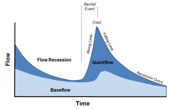
Figure 1Schematic representation of the rising limb and the falling limb (source: Environment Southland; https://www.es.govt.nz/environment/water/groundwater/groundwater-monitoring, last access: 2 April 2022).
The analysis employs a collection of indices drawn from hydrograph shape diagnoses, to extract information about the properties of rising and falling limbs of the hydrograph. The principle of time irreversibility is encapsulated by six streamflow indices that characterize the shape of a streamflow hydrograph.
The goals of this study are as follows: (i) to identify the key drivers of streamflow hydrograph (rising and falling limbs) in terms of catchment attributes (e.g., mean slope, aridity, fraction of precipitation falling as snow) using time-irreversibility-based indices; (ii) to present a spatial map-based attribute class based on streamflow indices for a large-sample hydrology dataset. The attribute class is a broad classification of attributes based on a particular aspect or feature. Topography, climate, and soil are examples of attribute classes. In this study, we present a new attribute class of streamflow indices related to rising and falling limbs, referred to as TI-streamflow indices (Time-irreversibility streamflow indices).
Hydrograph analysis is referred to as the investigation of the numerous factors that influence hydrograph shape (Rogers, 1972). The presence of hydrographs with a similar shape in long-term observation series of runoff suggests that the same conditions of runoff generation reoccur from time to time in the catchment of a river due to climate cyclicity and as a result of hydrological processes (Khrystyuk et al., 2017). Because climatic factors are dynamic in space and time, they seem to be the most significant factors influencing the hydrograph shape provided that changes in catchment conditions, such as land use are small. Khrystyuk et al. (2017) suggested that for the Desna river basin in Russia, temperature, snow water equivalent, and snowmelt conditions are the most critical factors influencing the shape of hydrographs; however, it is likely that these controls may not be equally important controls on hydrographs across all regions globally. The shape, timing, and peak flow of a streamflow hydrograph are influenced spatially and temporally by rainfall and watershed factors (Singh, 1997). One of the earlier studies by Roberts and Klingeman (1970) investigated the influence of meteorological and physiographic parameters on the runoff hydrograph using a physical laboratory model. Storm-related parameters (rainfall intensity, rainfall duration, storm movement) and basin surface conditions are among the inputs that could be experimentally modified in this model. The results revealed that each of these variables mentioned above has a substantial impact on the hydrograph shape where certain factors had a more considerable effect on the rising limb of the runoff hydrograph, whereas others were more important in terms of the flood crest (Roberts and Klingeman, 1970).
As shown in numerous studies in the literature, our notion of time-irreversibility and its indices could also be helpful in understanding the catchment drivers of streamflow hydrographs. This study presents an attribute class of hydrograph shape descriptors with temporal asymmetry. The significance of large-sample hydrology datasets in open hydrologic science and their potential to improve hydrologic study transparency is also underlined in this study.
Large-sample hydrology (LSH) gathers information from a large number of catchments to gain a more comprehensive understanding of hydrologic processes and to go beyond individual case studies. The LSH helps identify catchment behavior and leads one to derive precise conclusions regarding different hydrologic processes and models (Addor et al., 2020). Studies involving large-sample catchments help in understanding the drivers of hydrological change (Blöschl et al., 2019), in assessing hydrological similarity and classification (Berghuijs et al., 2014; Sawicz et al., 2014), in predictions in ungauged basins (Ehret et al., 2014), and in analyzing model and data uncertainty (Coxon et al., 2014) and foster hydrologic research by standardizing and automating the creation of large-sample hydrologic datasets worldwide (Addor et al., 2020). LSH assists in exploring interrelationships between numerous catchment attributes related to landscape, climate, and hydrology (Addor et al., 2017; Alvarez-Garreton et al., 2018; Gupta et al., 2014; Newman et al., 2015; Sawicz et al., 2011) and generalizing rules that can significantly improve the predictability of the water cycle (Alvarez-Garreton et al., 2018).
The primary challenges in fostering LSH are data availability and accessibility, which seriously hinder its use in data-scarce regions. Despite the fact that a few large-scale hydrologic studies have been undertaken, the number of publicly available large-scale datasets is still restricted (Addor et al., 2017, 2020; Coxon et al., 2020). Moreover, licensing restrictions and strict access policies make the datasets rarely available to the public (Coxon et al., 2020).
The model parameter estimation experiment (MOPEX) project dataset (Duan et al., 2006), the Canadian model parameter experiment (CANOPEX) database (Arsenault et al., 2016),the global streamflow indices and metadata archive (Do et al., 2018; Gudmundsson et al., 2018), global runoff reconstruction (Ghiggi et al., 2019), HydroATLAS (Linke et al., 2019) and the catchment attributes and meteorology for large-sample studies (CAMELS, Addor et al., 2017) are notable contributions of open and accessible large-sample catchment datasets (Coxon et al., 2020). The concept of time irreversibility-based streamflow indices is then applied to CAMELS catchments with the goal of encouraging large-sample hydrologic studies. The primary contribution of this study is to establish the distinction between signatures directly linked with rising limbs and falling limbs and their utility in uncovering processes associated with the hydrograph's steeply ascending and gradually descending limbs.
To facilitate an understanding of various hydrologic processes and streamflow hydrograph drivers, the study employs streamflow indices considering the streamflow hydrograph's temporal asymmetry. The descriptions of indices used in this study are tabulated in Table 1. Streamflow indices linked to each limb of the streamflow hydrograph within the time-irreversibility paradigm are distinguished since hydrographs have rising and falling limbs. The following indices are considered in the rising limb category: (1) rising limb density, (2) rising limb shape parameter, and (3) rising limb scale parameter. In contrast, (1) falling limb density (2) slope of upper recession (upper recession coefficient) (3) slope of lower recession (lower recession coefficient) are selected in the falling limb category. The next step is to compute these indices for a large number of catchments and correlate them with attributes such as climate, topography, vegetation, geology, and soil. The streamflow indices can be correlated explicitly since sub-categories are involved in each of the catchment attributes discussed above. Finally, the key attributes governing rising and falling limbs can be summarized and identified. The specifics of indices are explained further below.
Table 1Hydrologic descriptors with temporal asymmetry.
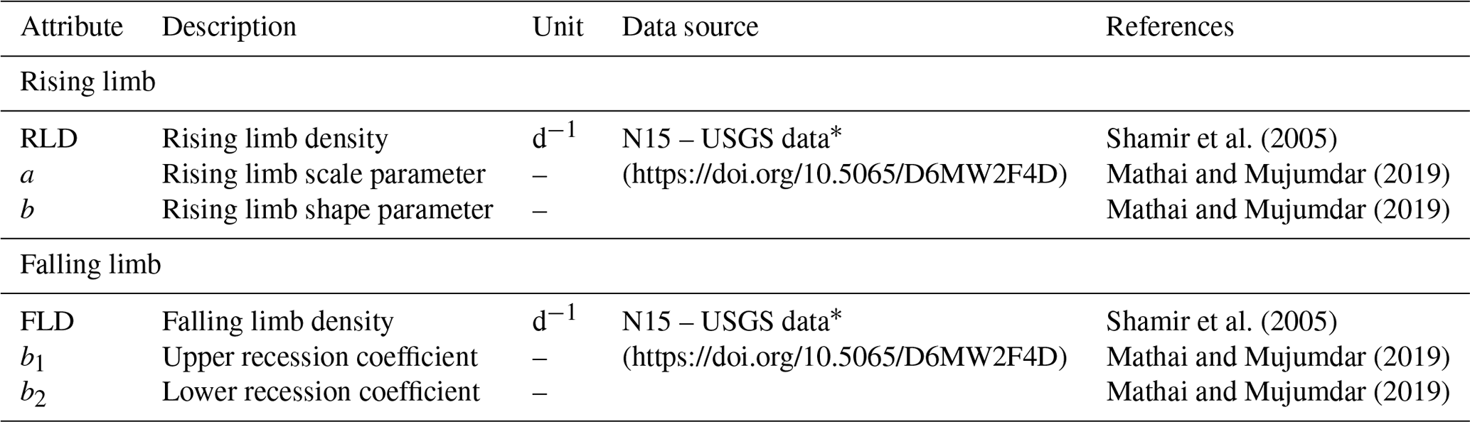
* N15 covers 671 catchments in the contiguous USA (CONUS), which provides daily meteorological forcing and daily streamflow measurements from the United States Geological Survey (USGS).
Rising limb density (RLD) is defined as the ratio of the number of rising limbs and the cumulative time of rising limbs (Shamir et al., 2005). The RLD is a hydrograph shape descriptor without considering the flow magnitude (Fig. 2) and the expression for RLD is given as:
The ratio of the number of falling limbs to the cumulative time of falling limbs is termed the falling limb density (FLD) (Fig. 2) (Shamir et al., 2005). The expression for FLD is given as:
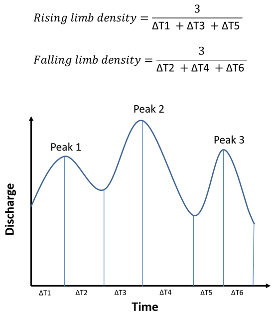
Figure 2Schematic example of rising limb density (RLD) and falling limb density (FLD) calculation (Shamir et al., 2005).
We first identify the hydrologic state of the stream (ascension and recession) (Mathai and Mujumdar, 2019). To determine the hydrologic state of a stream, increasing (wet) or decreasing (dry), on a given day, a time series of diurnal increments is extracted by differencing the original time series with its 1-day lagged time series. The positive increments are identified as diurnal increments for wet days (ascension limb).
To characterize the shape of the rising limbs occurring on wet days, the diurnal increments are fitted using an appropriate probability density function (PDF). The Weibull distribution satisfactorily reflects the diurnal increments of streamflow that occur on wet days (Mathai and Mujumdar, 2019; Stagge and Moglen, 2013; Szilagyi et al., 2006), and the scale “a” and shape “b” parameters of the Weibull distribution are computed for each catchment by using observed diurnal increments of streamflow (indicating δQ) of the ascension limb (Fig. 3a). The Weibull PDF is positive only for positive values of x, and is zero otherwise. For strictly positive values of the scale parameter a and shape parameter b, the density function is given by
where a>0, b>0. The shape and scale parameters of the Weibull distribution are estimated for each catchment from the observed diurnal increments of the streamflow. The scale parameter controls the magnitude of the rising limb, whilst the shape parameter reflects the flashiness of the rising limb. The scale parameter is related to the magnitude of storm events, which mirrors the general shape of flow in the stream. As a result, correlating these parameters with catchment attributes reveals which catchment attributes drive the magnitude and flashiness of rising limbs.
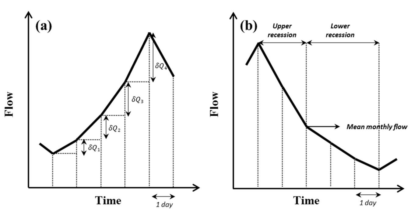
Figure 3Schematic representation of flow series (a) ascension limb and (b) recession limb (Mathai and Mujumdar, 2019).
In contrast, an exponential recession is used to capture the shape of the falling limbs on dry days of the daily hydrograph, representing the falling limbs' underlying dynamics (Mathai and Mujumdar, 2019). As the upper recession refers to the fast flow following a storm event and the lower recession refers to the base flow recession, falling limb modeling is done in two stages (Fig. 3b) (Aksoy, 2003; Aksoy and Bayazit, 2000). The steps to obtain recession coefficients b1 and b2 are explained below (Mathai and Mujumdar, 2019). To portray the shape of the recession limbs occurring on dry days of the daily hydrograph, an exponential recession is employed to capture the falling limbs' underlying dynamics (Mathai and Mujumdar, 2019). The expression for the exponential recession is given as follows:
where b is the recession coefficient, t is time, Qt is the flow t days after the peak and Q0 is the peak flow (Mathai and Mujumdar, 2019). Mean flow value is chosen as an appropriate measure (Sargent, 1979) to divide the recession into two stages. The limbs with a peak flow value greater than the observed mean flow value are considered as upper recessions and those with peak flow values smaller than the observed mean as lower recessions; however, it may be noted that using the mean monthly flow can lead to unusual situations if the peak flow for a given event is below the monthly mean. In such cases, the entire recession would be classified as a lower recession curve, and no upper part would exist. In those situations, there are still different driving processes for the first and second part of the recession, but these would all be lumped into one category in this case. Since we are dealing with the long-term time series, the recession slope will be nearly constant for a catchment and does not vary much with the recession separation technique used. In this study, we calculate recession slope at an annual scale. The upper recession is modeled as follows:
where b1 is the recession coefficient for the upper part of the recession limb, t is the number of days after the peak, Qt is flow t days after the peak, Q0 is the preceding peak flow (Mathai and Mujumdar, 2019). The lower recession is represented as:
where b2 is the recession coefficient for the lower part of the recession limb, t* is the time from the start of the lower recession and is the initial flow in the lower part of the recession (Mathai and Mujumdar, 2019). The recession expressions for upper and lower recessions are fitted by regressing ) versus t and versus respectively. These linear regressions are performed on each individual recession sequence. The average of the upper and/or lower recession parameters is taken as the upper or lower recession parameter of that catchment (on daily time series data).
The study uses indices related to rising limb (viz., RLD, rising limb scale parameter, rising limb shape parameter) and recession limb (viz., FLD, upper recession coefficient, lower recession coefficient) to summarize the characteristic shape of steeply ascending and gradually descending limbs and its application in understanding the role of various drivers of catchment attributes in streamflow generation.
Section 3 provides the description of the dataset used and the study area chosen. This study employs the CAMELS dataset, which encompasses daily discharge data and catchment attributes for 671 catchments (Fig. 4) across the continental United States, representing a diverse set of catchments with long streamflow time series covering a wide range of hydroclimatic conditions (Addor et al., 2017). The time frame chosen for the analysis is from 1 October 1989 to 30 September 2009 (Addor et al., 2017).
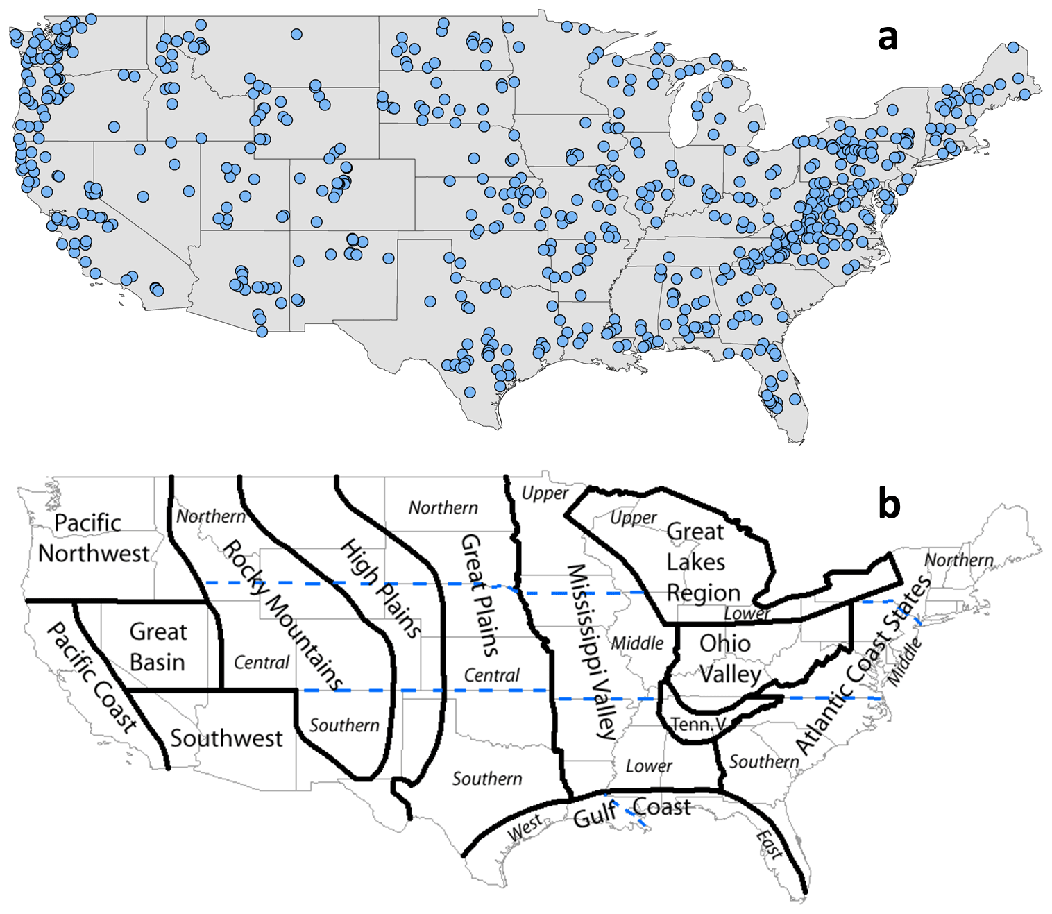
Figure 4(a) Map of 671 CAMELS catchments in the continental US considered in this study. (b) Geographical regions of the US according to NOAA National Centers for Environmental Information referred for the analysis (source: NOAA National Centers for Environmental Information; https://www.ncdc.noaa.gov/temp-and-precip/drought/nadm/geography, last access: 2 April 2022).
The topographic characteristics of the CAMELS dataset are represented in Fig. S1 in the Supplement. Except for the Appalachian Mountains, the eastern part of the continental United States is much flatter than the western portion, according to mean elevation and mean slope maps (Fig. S1a and b). Figure S1c depicts the spatial pattern of catchment size, highlighting the presence of some catchments with an area greater than 10 000 km2. The landscape of each catchment is described using multiple attributes, which can be divided into various classes as shown in Table S1 in the Supplement (Addor et al., 2017).
The regional variability of the streamflow indices is investigated by computing the rising limb density, falling limb density, rising limb scale parameter, rising limb shape parameter, upper recession coefficient, and lower recession coefficient for 671 CAMELS catchments and given as spatial maps. These spatial maps of streamflow indices complement CAMELS' six main classes of catchment attributes developed (Addor et al., 2017): topography, climate, streamflow, land cover, soil, and geology. The motivation for presenting streamflow indices in the form of spatial maps with respect to geographical regions is to align with spatial maps introduced by the CAMELS dataset. In addition, streamflow indices are also presented in hydrologic clusters to incorporate a more explicit spatial representation of catchment behavior across the CONUS. The hydrologic clusters are used to link the current study to the existing catchment classification literature undertaken in the CONUS region.
As catchment attributes cover a broad range of aspects of catchment hydrology such as land cover, soil, climate, geology, topography, and each of the attributes usually does not exist independently in space but is closely interlinked, resulting in various strongly correlated attributes in a catchment (Jehn et al., 2020; Stein et al., 2021), the association between these attributes and streamflow indices is discussed further in the subsequent section. The scope of this work is limited as it does not attempt to explain all interrelations between each attribute; instead, the main objective of the study is to establish the governing catchment attributes of streamflow indices.
Furthermore, previous studies revealed that climate attributes significantly influence catchment streamflow dynamics; hence, it is crucial to understand the role of different climatic zones on these six streamflow indices (Addor et al., 2018; Berghuijs et al., 2014; Jehn et al., 2020; Knoben et al., 2018; Stein et al., 2021). Since the chosen 671 catchments are distributed across the US in various climatic zones (Jehn et al., 2020; Knoben et al., 2018; Stein et al., 2021), the CAMELS dataset is ideal for addressing this question. With this motivation, the effect of climate attributes on streamflow indices associated with rising and falling limbs is also investigated in the last section.
4.1 Spatial variability in streamflow indices and relation of the streamflow indices with catchment attributes
Streamflow indices related to rising limbs and falling limbs are computed for the selected catchments and displayed in spatial maps as shown in Figs. 5 and 7, respectively. The spatial analysis is based on the US geographical areas (for details, refer to Fig. 4b) as defined by the NOAA National Centers for Environmental Information and is referred to in the following spatial maps. Furthermore, the clusters provided by Jehn et al. (2020) to represent the discrete hydrological behaviors of the continental United States are adopted in this study to understand the regional variability of catchment behavior. Figure S2 and Table S2 present the location map and details of the 10 clusters. Figure S3 shows boxplots of the catchment attributes of the clusters (after Jehn et al., 2020).
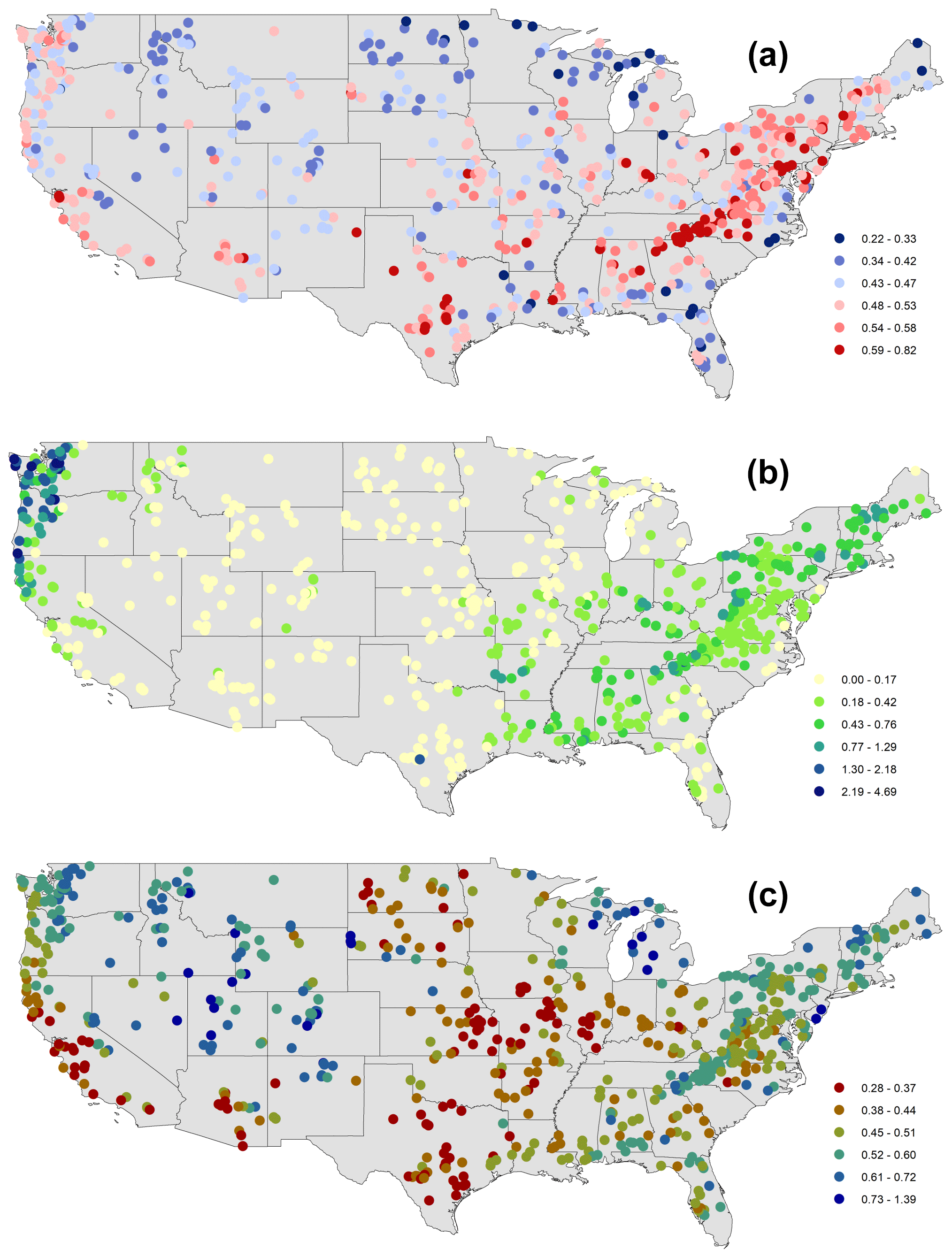
Figure 5Spatial maps of streamflow indices associated with a rising limb (a) rising limb density [d−1], (b) rising limb scale parameter, (c) rising limb shape parameter over the CONUS.
Even though a comprehensive dataset such as CAMELS provides an excellent overview of various catchments in contrasting climatic and topographic regions, it does not by itself provide insights to explain hydrologic behavior. We present here streamflow indices in clusters representing distinct hydrologic behavior, enabling an understanding of the hydrologic processes. Jehn et al. (2020) summarizes the characteristics of each catchment cluster in terms of climate, hydrology and location. The clusters presented by Jehn et al. (2020) are formed based on agglomerative hierarchic clustering with ward linkage on the principal components of the hydrologic signatures. The hydrolog signatures identified with the highest spatial predictability are used to cluster 643 catchments from the CAMELS dataset (Jehn et al., 2020). This facilitates straightforward interpretations of the observations to explain the hydrologic behavior in each cluster.
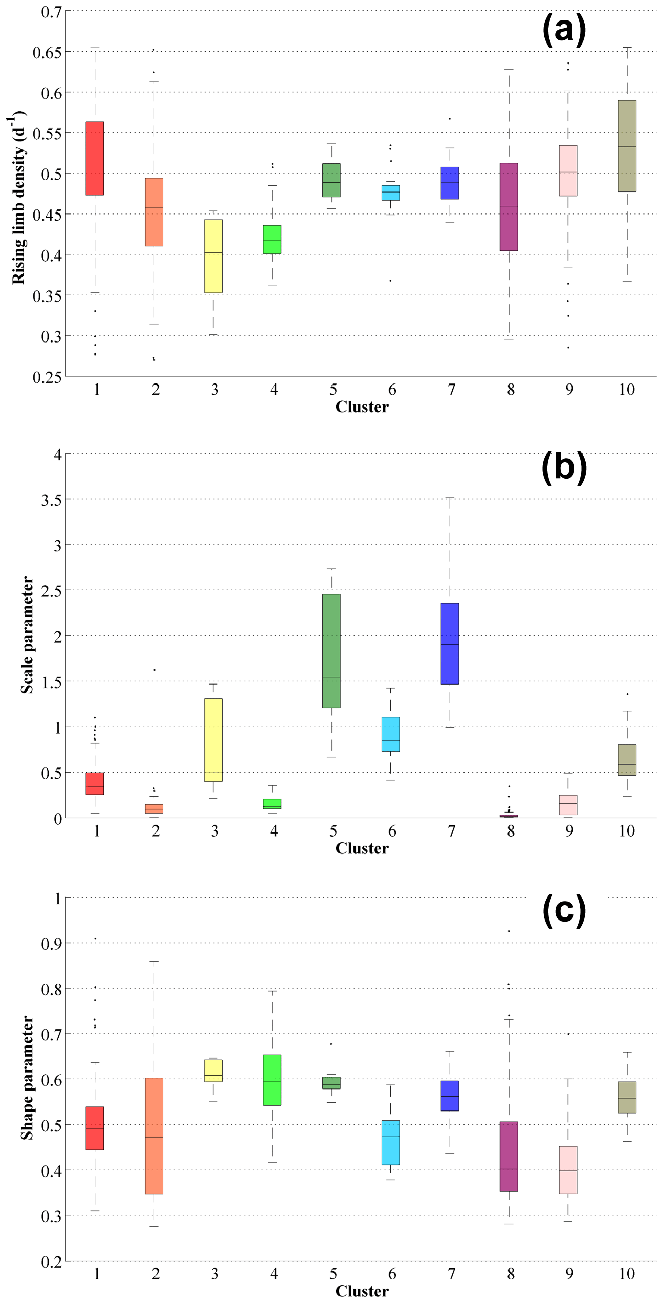
Figure 6Boxplots of the hydrological descriptors linked with the rising limb (a) rising limb density [d−1], (b) rising limb scale parameter, (c) rising limb shape parameter of the clusters over the CONUS.
In this paper, we first identify the regions in the US where high and low values of streamflow indices occur. The dominant catchment attributes of these regions are also identified using corresponding clusters. The streamflow indices and the dominant catchment attribute are then related to interpreting the findings obtained. In terms of geographical regions, the rising limb density is highest over the Atlantic Coast States, Ohio Valley, Lower Mississippi Valley, Southern Great Plains, Southwest and Pacific, and lowest along the Upper Great Lakes Region, Upper Mississippi Valley, Great Basin, and Northern Rocky Mountains, Northern Interior Plains, and the East Gulf Coast (Fig. 5a). Furthermore, in terms of hydrologic clusters, the Appalachian Mountains (cluster 10), Southeastern and Central plains (cluster 1), and all southernmost states of the US (cluster 9) witness high rising limb densities (Fig. 6a). Cluster 1 is characterized by high forest fraction and low elevation (Figure S3), resulting in little annual snowfall. Cluster 10 catchments are located in the Appalachian Mountains (Fig. S2), with a higher mean elevation than most other clusters, experiencing low aridity and high forest cover (Fig. S3); however, cluster 9 encompasses all of the southern US states, with negative precipitation seasonality (winter) and higher forest cover and green vegetation (Fig. S3). Furthermore, all of the catchments in cluster 9 are very near the sea (Fig. S2), with a low snow component and high evapotranspiration (Fig. S3). We used Spearman rank correlation for the correlation analysis, shown in Table 2. It can be seen that the rising limb density shows a negative correlation (Table 2) with the area (), elevation () fraction of precipitation falling as snow (), and depth to bedrock (). Northwestern forested mountains (clusters 3 and 4), located in the mountains of the western US, experience low values of rising limb density. The catchments of cluster 3 have a high fraction of precipitation falling as snow (Fig. S3). Cluster 4 is found in the western US mountains (Fig. S2), where there is a lot of snow, the same as cluster 3 (Fig. S3). Low values of rising limb density are observed due to a negative correlation with the fraction of precipitation falling as snow () (Table 2). The study indicates that rising limb density is mainly governed by elevation and fraction of precipitation falling as snow in the CONUS.
Table 2Correlation (r-values) between streamflow indices and the catchment attributes. Corresponding (p-values) are shown in brackets. Insignificant correlations (p>0.05) are marked in italics.
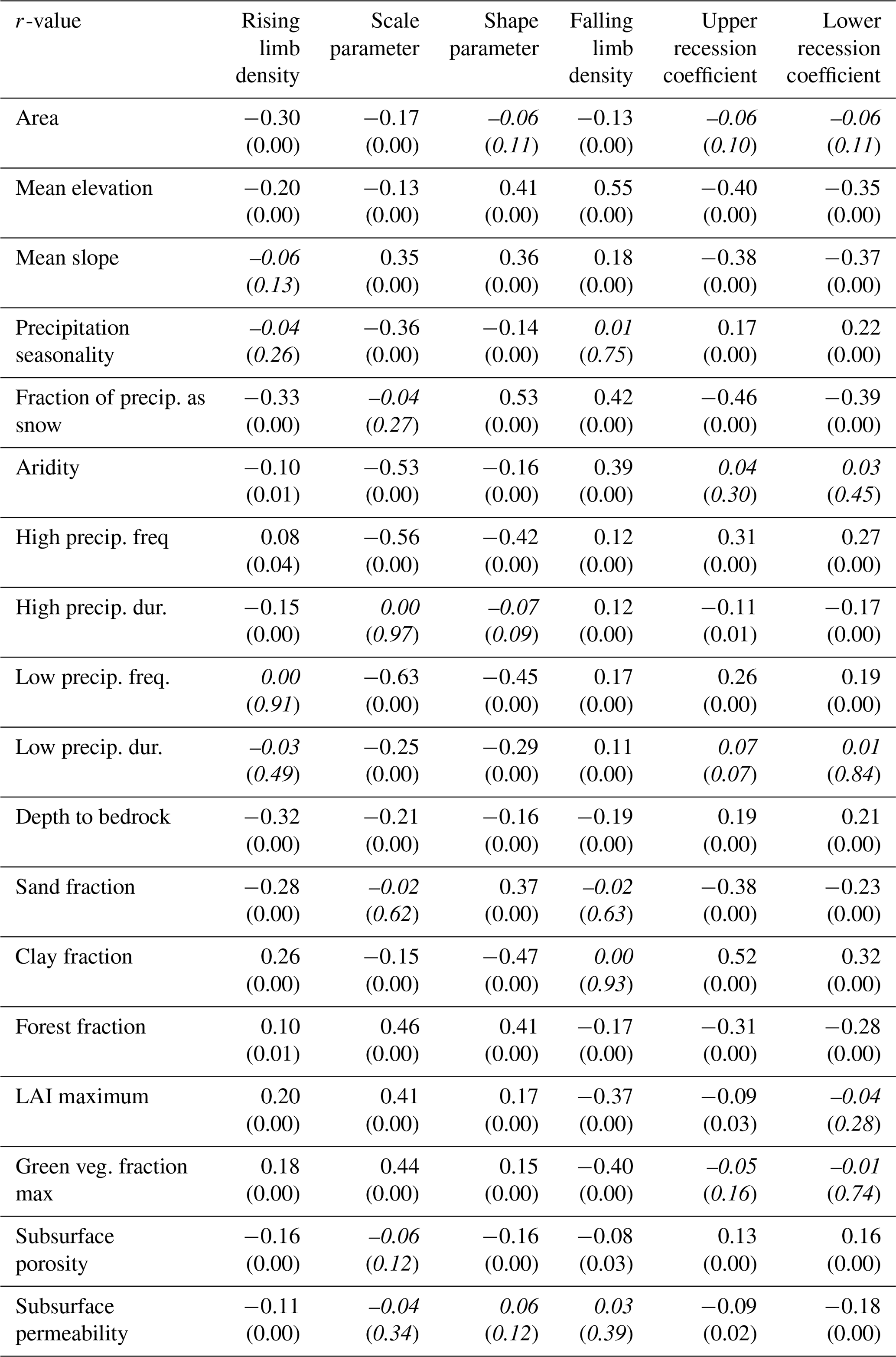
Considerably low values of rising limb scale parameters are experienced over the Rocky Mountains, High Plains, Great Plains, Upper Mississippi Valley, Great Basin, Southwest, and the Great Lakes Regions, whereas the Pacific Northwest shows high values of rising limb scale parameters (Fig. 5b). Clusters (5, 7) over the northwestern forested mountains of CONUS (Fig. S2) experience very high values of rising limb scale parameters (Fig. 6b). These catchments have the highest discharge, especially in the early summer, due to a combination of high precipitation and snowmelt (Jehn et al., 2020). Furthermore, the region in the continental US which receives the highest precipitation is included in cluster 5 (Jehn et al., 2020). Moreover, cluster 5 consists of a large proportion of forest (Fig. S3). Again, cluster 7 with high values of rising limb scale parameter (Fig. 6b) is characterized by reasonably high fraction of precipitation falling as snow (Fig. S3). High precipitation and snowmelt might result in a large discharge. Higher discharges can create higher values of rising scale parameters as the rising limb scale parameter regulates the magnitude of the rising limb. Low values of rising limb scale parameters are shown by clusters 2, 8, 9 (Fig. 6b). This is because of low water availability, low snow fraction precipitation falling as snow, and high evaporation experienced in these regions (Jehn et al., 2020). Low discharge and thus lower rising limb scale parameters can be caused by excessive evaporation, low water availability, and a low snow fraction of precipitation falling as snow. It is observed that the rising limb scale parameter (Table 2) shows a negative correlation with climate ( for aridity) and a positive association with the vegetation attributes (r=0.46 for forest fraction, r=0.41 for leaf area index (LAI) maximum, r=0.44 for green vegetation fraction maximum). Frequency of precipitation ( for high precipitation frequency, for low precipitation frequency) displays a strong negative association with the rising limb scale parameter (Table 2).
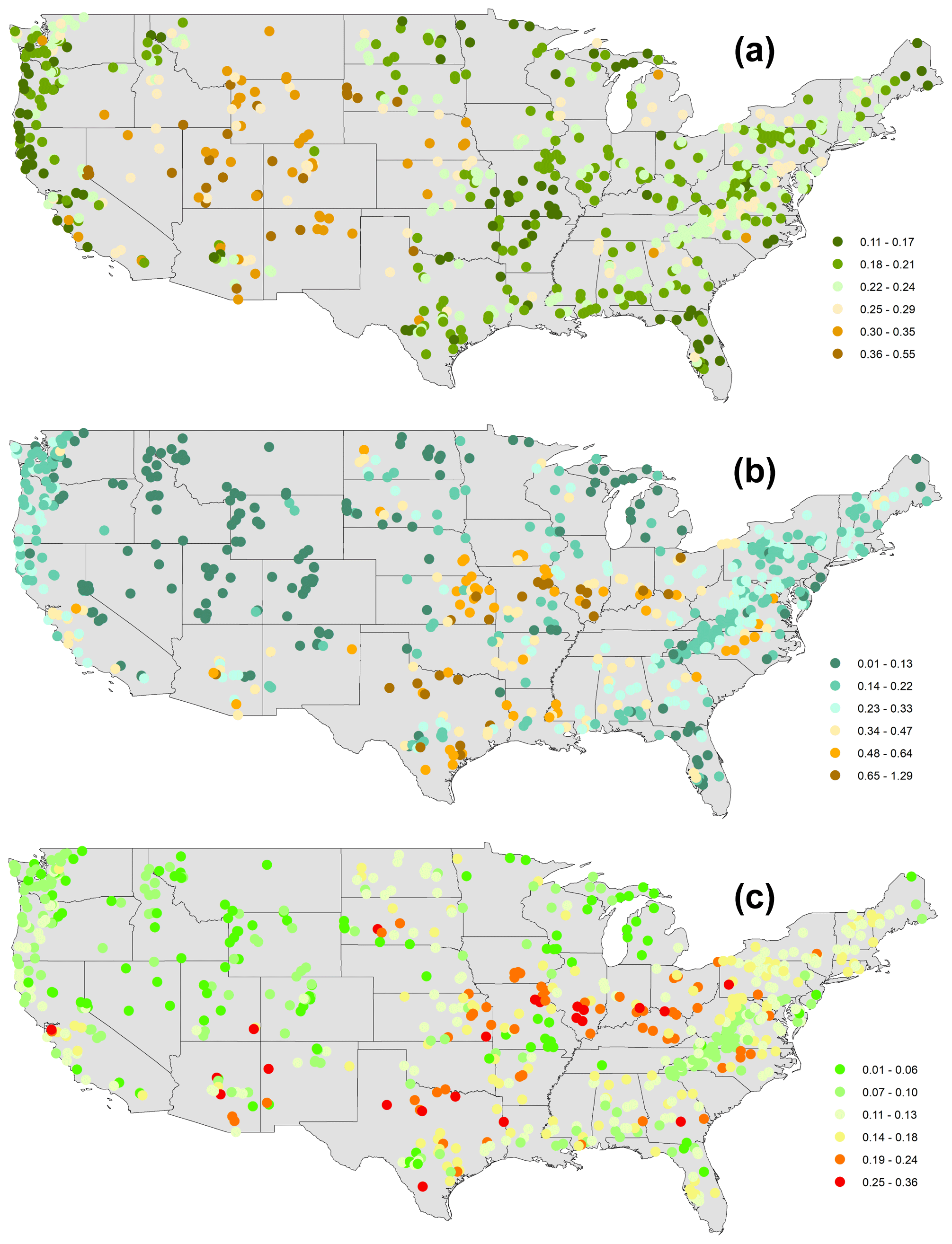
Figure 7Regional variability of streamflow indices associated with the falling limb (a) falling limb density [d−1], (b) upper recession coefficient, (c) lower recession coefficient over the CONUS.
Low rising limb shape parameter occurs along the Great Plains, Mississippi Valley, Pacific Coast, and the west of the Gulf Coast (Fig. 5c). In contrast, the shape parameter over the Rocky Mountains, High Plains, Great Basin, Pacific Northwest, and the Great Lakes Region witnesses the highest values of rising limb shape parameters (Fig. 5c). All the catchments located in the southern states of the US (cluster 9), Great Plains and North American deserts (cluster 8), and the Central Plains (cluster 2) characterize low values of rising limb shape parameters (Fig. 6c). This is due to low water availability, low snow fraction precipitation falling as snow, low leaf area index, and high evaporation experienced in these regions (Jehn et al., 2020). Excessive evaporation and a low snow fraction of precipitation falling as snow can contribute to low discharge and thus lower rising limb shape parameters. It is noted that the rising limb shape parameter indicates (Table 2) a positive correlation with vegetation attributes (r=0.41 for forest fraction) and the fraction of precipitation falling as snow (r=0.53), mean slope (r=0.36), mean elevation (r=0.41), and sand fraction (r=0.37) whereas, it negatively correlates with precipitation frequency ( for high precipitation frequency and for low precipitation frequency). High values of rising limb shape parameters are seen in clusters 3, 4 (Fig. 6c) located in the northwestern forested mountains of the western US (Fig. S2), dominant with a summer peak of discharge caused by rapid snowmelt. The rapid snowmelt can cause flashy hydrographs with high values of rising limb shape parameters.
Catchments with a high falling limb density are predominantly located along the Great Basin and the Rocky Mountains and in the High Plains region (Fig. 7a). This is due to less forest cover in these arid regions and falling limb density shows a positive association with the arid climate (r=0.39) (Table 2). Clusters 6, 7 (Fig. 8a) over marine West Coast forests and Western Cordillera (Table S2) experience smaller falling limb densities. We can see that falling limb density is mainly governed by climate indices and is negatively correlated with the land cover characteristics (for LAI maximum () and green veg. fraction max (), Table 2). Mean elevation (r=0.55) also strongly characterizes the nature of the falling limb density (Table 2). Besides, fraction of precipitation falling as snow (r=0.42) is also positively correlated with falling limb density (Table 2).
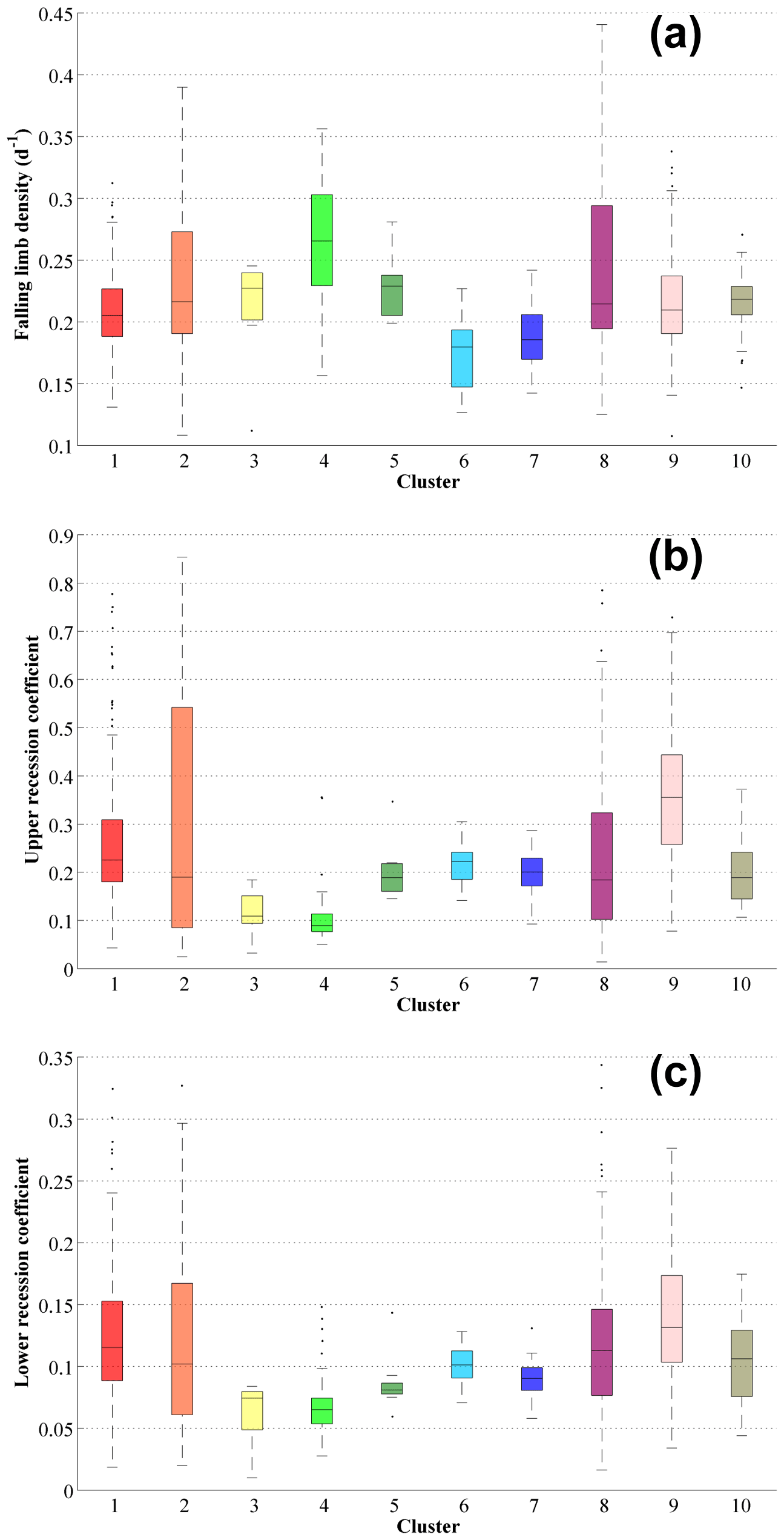
Figure 8Boxplots of the streamflow indices related with the falling limb (a) falling limb density [d−1], (b) upper recession coefficient, (c) lower recession coefficient of the clusters.
Similarities exist between the patterns of the upper recession coefficient and the lower recession coefficient (Fig. 7b and c). Clusters 3, 4 located in the northwestern forested mountains (Fig. S2), which have overall low discharge, show low values of upper and lower recession coefficients (Fig. 8b and c). Clusters 2 and 9, located in the eastern US, witness high values of recession coefficients; due to low slope inclinations (Jehn et al., 2020), water takes a long time to reach the outlet (Fig. 8b and c). Recession coefficients are negatively correlated (Table 2) with topographic indices (with mean elevation: upper_r = −0.40, lower_r = −0.35; with mean slope: upper_r = −0.38, lower_r = −0.37, where upper_r and lower_r corresponds to correlation values of upper and lower recession coefficients, respectively). Furthermore, the recession coefficients show a positive correlation with clay (upper_r = 0.52, lower_r = 0.32) and negative correlations with the fraction of precipitation falling as snow (upper_r = −0.46, lower_r = −0.39), forest fraction (upper_r = −0.31, lower_r = −0.28), and sand fraction (upper_r = −0.38, lower_r = −0.23, Table 2). Moreover, the geology attributes such as subsurface porosity (upper_r = 0.13, lower_r = 0.16) reveal a positive correlation to recession coefficients and a negative (upper_r = −0.09, lower_r = −0.18) with subsurface permeability (Table 2).
4.2 Influence of attributes of climate to streamflow indices
The climatic indices indicate a more substantial influence on hydrologic signatures than the topographic, soil, land cover, and geological attributes combined (Addor et al., 2018; Stein et al., 2021). Additionally, the findings of Jehn et al. (2020) highlighted that the climate appears to be the most critical factor influencing hydrologic behavior in the CAMELS dataset. Hence, the streamflow indices are examined in the climate index space (aridity along x-axis and fraction of precipitation falling as snow along the y-axis) to evaluate the main drivers of the catchments. Single dots show the catchments and are colored by their hydrological clusters (Fig. 9a).

Figure 9(a) Comparison of the hydrologic clusters of Jehn et al. (2020) with the climate index space (fraction of precipitation falling as snow vs. aridity). Single dots show the catchments and are colored by their hydrologic clusters. Comparison of the streamflow indices in climate index space, (b) rising limb density, (c) rising limb scale parameter, (d) rising limb shape parameter, (e) falling limb density, (f) upper recession coefficient, (g) lower recession coefficient for all catchments. Single dots show the catchments and are colored according to the value of the streamflow indices.
Clusters 1, 5, 6, 7, 10 are characterized by a low fraction of precipitation falling as snow and humid climate, whereas clusters 3, 4 have humid climates experiencing a high fraction of precipitation falling as snow (Fig. 9a). Clusters 2, 8, 9 are featured by a low fraction of precipitation falling as snow and arid climate (Fig. 9a). The three categories mentioned above are referred to as G1, G2, and G3, respectively.
Clusters G1 with a low fraction of precipitation falling as snow with humid climate show (clusters 1, 9, 10) high rising limb densities (Fig. 9b) and (clusters 5, 7) high rising limb scale parameters (Fig. 9c). This is because the rising limb density negatively correlates with the fraction of precipitation falling as snow (Table 2: , Fig. 9b), whereas the rising limb scale parameter negatively correlates with aridity (Table 2: , Fig. 9c). Moreover, these clusters G1 experience a low value of (clusters 6, 7) falling limb density (Fig. 9e). This is because the falling limb density positively correlates with the climate indices (Table 2: r=0.42 for fraction of precipitation falling as snow and r=0.39 for aridity, Fig. 9e).
As mentioned earlier, clusters G2 with humid climates and with a high fraction of precipitation falling as snow (clusters 3, 4) display low values of rising limb density as rising limb density correlates negatively with the fraction of precipitation falling as snow (Table 2: , Fig. 9b). Cluster G2 witnesses higher values of rising limb shape parameter due to its negative correlation with aridity () and positive correlation with the fraction of precipitation falling as snow (Table 2: r=0.53, Fig. 9d). Furthermore, the clusters of G2 (clusters 3, 4) show low values of recession coefficients as they depict a strong negative correlation with the fraction of precipitation falling as snow (Table 2: upper_r = −0.46, and lower_r = −0.39, Fig. 9f and g).
Low values of rising limb scale and shape parameters are noticed for the clusters 2, 8, 9 (clusters G3) with arid climate and low fraction of precipitation falling as snow (Fig. 9c and d) due to its negative correlation with aridity as stated earlier. Cluster 8 experiences the maximum values of falling limb density (Fig. 9e) where the region witnesses low fraction of snow and arid catchments, due to its strong positive correlates with the aridity (r=0.39, Table 2).
Streamflow hydrographs portray the time distribution of runoff at the point of measurement by a single curve, and the hydrographs are characterized by their time irreversibility property. In this study, the indices related to this characteristic feature are used to study the catchment drivers of streamflow hydrographs. The streamflow indices associated with the time irreversibility of hydrographs open new opportunities to investigate the interaction between topography, soil, climate, vegetation, geology that drive the hydrologic behavior of catchments. Moreover, most of the previously presented hydrologic indices are employed only for time-symmetric processes (McMillan, 2021); the importance of the time irreversibility of streamflow is highlighted in this study. The indices associated with rising and falling limbs are primarily correlated to distinct catchment attributes, establishing a relationship between the indices and catchment attributes, such as climate, topography, soil, geology, and vegetation to delineate the controlling drivers in corresponding hydrograph sections. A set of streamflow indices with temporal asymmetry for 671 catchments in the US is presented in this study. The regional variations among catchments over the US are compared and discussed using the spatial maps of streamflow indices. Such spatial maps of the streamflow indices supplement the hydrometeorologic time series and catchment attributes provided by Addor et al. (2017).
The study showed that the rising limb density is mainly governed by the elevation and fraction of precipitation falling as snow. Climate indices, mean elevation, and the fraction of precipitation falling as snow mainly influence falling limb density. In contrast, the aridity and frequency of precipitation drive the rising limb scale parameter. Furthermore, forest fraction, the fraction of precipitation falling as snow, mean slope, mean elevation, sand fraction, and precipitation frequency influence the rising limb shape parameter. Mean elevation, mean slope, clay, the fraction of precipitation falling as snow, forest fraction, and sand fraction all determine recession coefficients. Finally, streamflow indices are studied in the climate index space to isolate the leading drivers of runoff generation. High rising limb densities and rising limb scale parameters are observed in catchments with low precipitation falling as snow and a humid climate. It is observed that the catchments with a humid climate and a high fraction of precipitation falling as snow display low values of rising limb density, high values of the rising limb shape parameter, and low values of recession coefficients. The lowest values of rising limb scale and shape parameters, and the highest values of falling limb density, are seen in catchments of arid climates and a low fraction of precipitation falling as snow.
In general, the contribution of this work lies in differentiating hydrographs depending on their time irreversibility property and using the corresponding indices to provide an alternative methodology for identifying the drivers of streamflow hydrographs. In the context of large sample hydrologic research, the concept of time-irreversibility and the indices associated with it could also be used to describe the drivers at catchment scale. It must be noted that each attribute (e.g., climate vegetation, soil, geology) usually does not exist alone in space but is closely interwoven, resulting in strongly correlated attributes in a catchment (Jehn et al., 2020; Stein et al., 2021); however, it would be beyond the scope of this paper to describe all probable relationships between attributes. Keeping this in mind, the main focus of this study was constrained to only identify the controlling attributes of streamflow indices. Another limitation of the work is related with the characterization of recessions used. Future work may investigate using the inflection point or another recession separation technique to characterize recessions.
The CAMELS dataset can be found at https://doi.org/10.5194/hess21-5293-2017 (Addor et al., 2017). The hydrometeorologic time series (https://doi.org/10.5065/D6MW2F4D; Newman et al., 2014) used in this paper are freely available online.
The supplement related to this article is available online at: https://doi.org/10.5194/hess-26-2019-2022-supplement.
JM conceptualized the work, developed the methodology, and carried out the data curation, formal analysis, validation, and writing of the original draft. PPM reviewed the initial manuscript and provided the resources needed for this work.
The contact author has declared that neither they nor their co-author has any competing interests.
Publisher's note: Copernicus Publications remains neutral with regard to jurisdictional claims in published maps and institutional affiliations.
We would like to thank all the people who created the CAMELS dataset. We sincerely thank Elena Toth (editor), Wouter Knoben, and the anonymous reviewer for patiently reviewing the paper and offering valuable critical comments. Their suggestions have significantly improved the quality of our paper.
The funding received from the Ministry of Earth Sciences (MoES), Government of India, through the project, “Advanced Research in Hydrology and Knowledge Dissemination”, Project No.: MOES/PAMC/H&C/41/2013-PC-II, is gratefully acknowledged.
The Ministry of Earth Sciences, Government of India, has supported this research through the project “Advanced Research in Hydrology and Knowledge Dissemination” (grant no. MOES/PAMC/H&C/41/2013-PC-II).
This paper was edited by Elena Toth and reviewed by Wouter Knoben and one anonymous referee.
Addor, N., Newman, A. J., Mizukami, N., and Clark, M. P.: The CAMELS data set: catchment attributes and meteorology for large-sample studies, Hydrol. Earth Syst. Sci., 21, 5293–5313, https://doi.org/10.5194/hess-21-5293-2017, 2017.
Addor, N., Nearing, G., Prieto, C., Newman, A. J., Le Vine, N., and Clark, M. P.: A Ranking of Hydrological Signatures Based on Their Predictability in Space, Water Resour. Res., 54, 8792–8812, https://doi.org/10.1029/2018WR022606, 2018.
Addor, N., Do, H. X., Alvarez-Garreton, C., Coxon, G., Fowler, K., and Mendoza, P. A.: Large-sample hydrology: recent progress, guidelines for new datasets and grand challenges, Hydrolog. Sci. J., 65, 712–725, https://doi.org/10.1080/02626667.2019.1683182, 2020.
Aksoy, H.: Markov chain-based modeling techniques for stochastic generation of daily intermittent streamflows, Adv. Water Resour., 26, 663–671, https://doi.org/10.1016/S0309-1708(03)00031-9, 2003.
Aksoy, H. and Bayazit, M.: A Daily Intermittent Streamflow Simulator, Turkish J. Eng. Environ. Sci., 24, 265–276, 2000.
Aksoy, H., Bayazit, M., and Wittenberg, H.: Probabilistic approach to modelling of recession curves, Hydrolog. Sci. J., 46, 269–285, 2001.
Alvarez-Garreton, C., Mendoza, P. A., Boisier, J. P., Addor, N., Galleguillos, M., Zambrano-Bigiarini, M., Lara, A., Puelma, C., Cortes, G., Garreaud, R., McPhee, J., and Ayala, A.: The CAMELS-CL dataset: catchment attributes and meteorology for large sample studies – Chile dataset, Hydrol. Earth Syst. Sci., 22, 5817–5846, https://doi.org/10.5194/hess-22-5817-2018, 2018.
Arsenault, R., Bazile, R., Ouellet Dallaire, C., and Brissette, F.: CANOPEX: A Canadian hydrometeorological watershed database, Hydrol. Process., 30, 2734–2736, https://doi.org/10.1002/hyp.10880, 2016.
Berghuijs, W. R., Sivapalan, M., Woods, R. A., and Savenije, H. H. G.: Patterns of similarity of seasonal water balances: A window into streamflow variability over a range of time scales, Water Resour. Res., 50, 5638–5661, https://doi.org/10.1002/2014WR015692, 2014.
Blöschl, G., Hall, J., Viglione, A., Perdigão, R. A. P., Parajka, J., Merz, B., Lun, D., Arheimer, B., Aronica, G. T., Bilibashi, A., Boháč, M., Bonacci, O., Borga, M., Čanjevac, I., Castellarin, A., Chirico, G. B., Claps, P., Frolova, N., Ganora, D., Gorbachova, L., Gül, A., Hannaford, J., Harrigan, S., Kireeva, M., Kiss, A., Kjeldsen, T. R., Kohnová, S., Koskela, J. J., Ledvinka, O., Macdonald, N., Mavrova-Guirguinova, M., Mediero, L., Merz, R., Molnar, P., Montanari, A., Murphy, C., Osuch, M., Ovcharuk, V., Radevski, I., Salinas, J. L., Sauquet, E., Šraj, M., Szolgay, J., Volpi, E., Wilson, D., Zaimi, K., and Živković, N.: Changing climate both increases and decreases European river floods, Nature, 573, 108–111, https://doi.org/10.1038/s41586-019-1495-6, 2019.
Clark, M. P., McMillan, H. K., Collins, D. B. G., Kavetski, D., and Woods, R. A.: Hydrological field data from a modeller's perspective: Part 2: Process-based evaluation of model hypotheses, Hydrol. Process., 25, 523–543, https://doi.org/10.1002/hyp.7902, 2011.
Coxon, G., Freer, J., Wagener, T., Odoni, N. A., and Clark, M.: Diagnostic evaluation of multiple hypotheses of hydrological behaviour in a limits-of-acceptability framework for 24 UK catchments, Hydrol. Process., 28, 6135–6150, https://doi.org/10.1002/hyp.10096, 2014.
Coxon, G., Addor, N., Bloomfield, J. P., Freer, J., Fry, M., Hannaford, J., Howden, N. J. K., Lane, R., Lewis, M., Robinson, E. L., Wagener, T., and Woods, R.: CAMELS-GB: hydrometeorological time series and landscape attributes for 671 catchments in Great Britain, Earth Syst. Sci. Data, 12, 2459–2483, https://doi.org/10.5194/essd-12-2459-2020, 2020.
Do, H. X., Gudmundsson, L., Leonard, M., and Westra, S.: The Global Streamflow Indices and Metadata Archive (GSIM) – Part 1: The production of a daily streamflow archive and metadata, Earth Syst. Sci. Data, 10, 765–785, https://doi.org/10.5194/essd-10-765-2018, 2018.
Duan, Q., Schaake, J., Andréassian, V., Franks, S., Goteti, G., Gupta, H. V., Gusev, Y. M., Habets, F., Hall, A., Hay, L., Hogue, T., Huang, M., Leavesley, G., Liang, X., Nasonova, O. N., Noilhan, J., Oudin, L., Sorooshian, S., Wagener, T., and Wood, E. F.: Model Parameter Estimation Experiment (MOPEX): An overview of science strategy and major results from the second and third workshops, J. Hydrol., 320, 3–17, https://doi.org/10.1016/j.jhydrol.2005.07.031, 2006.
Ehret, U., Gupta, H. V., Sivapalan, M., Weijs, S. V., Schymanski, S. J., Blöschl, G., Gelfan, A. N., Harman, C., Kleidon, A., Bogaard, T. A., Wang, D., Wagener, T., Scherer, U., Zehe, E., Bierkens, M. F. P., Di Baldassarre, G., Parajka, J., van Beek, L. P. H., van Griensven, A., Westhoff, M. C., and Winsemius, H. C.: Advancing catchment hydrology to deal with predictions under change, Hydrol. Earth Syst. Sci., 18, 649–671, https://doi.org/10.5194/hess-18-649-2014, 2014.
Ghiggi, G., Humphrey, V., Seneviratne, S. I., and Gudmundsson, L.: GRUN: an observation-based global gridded runoff dataset from 1902 to 2014, Earth Syst. Sci. Data, 11, 1655–1674, https://doi.org/10.5194/essd-11-1655-2019, 2019.
Gudmundsson, L., Do, H. X., Leonard, M., and Westra, S.: The Global Streamflow Indices and Metadata Archive (GSIM) – Part 2: Quality control, time-series indices and homogeneity assessment, Earth Syst. Sci. Data, 10, 787–804, https://doi.org/10.5194/essd-10-787-2018, 2018.
Gupta, H. V., Perrin, C., Blöschl, G., Montanari, A., Kumar, R., Clark, M., and Andréassian, V.: Large-sample hydrology: a need to balance depth with breadth, Hydrol. Earth Syst. Sci., 18, 463–477, https://doi.org/10.5194/hess-18-463-2014, 2014.
Jehn, F. U., Bestian, K., Breuer, L., Kraft, P., and Houska, T.: Using hydrological and climatic catchment clusters to explore drivers of catchment behavior, Hydrol. Earth Syst. Sci., 24, 1081–1100, https://doi.org/10.5194/hess-24-1081-2020, 2020.
Khrystyuk, B., Gorbachova, L., and Koshkina, O.: The impact of climatic conditions of spring flood formation on hydrograph shape of the Desna River, Meteorol. Hydrol. Water Manage., 5, 63–70, https://doi.org/10.26491/mhwm/67914, 2017.
Knoben, W. J. M., Woods, R. A., and Freer, J. E.: A Quantitative Hydrological Climate Classification Evaluated With Independent Streamflow Data, Water Resour. Res., 54, 5088–5109, https://doi.org/10.1029/2018WR022913, 2018.
Koutsoyiannis, D.: Simple stochastic simulation of time irreversible and reversible processes, Hydrolog. Sci. J., 65, 536–551, https://doi.org/10.1080/02626667.2019.1705302, 2020.
Kuentz, A., Arheimer, B., Hundecha, Y., and Wagener, T.: Understanding hydrologic variability across Europe through catchment classification, Hydrol. Earth Syst. Sci., 21, 2863–2879, https://doi.org/10.5194/hess-21-2863-2017, 2017.
Linke, S., Lehner, B., Ouellet Dallaire, C., Ariwi, J., Grill, G., Anand, M., Beames, P., Burchard-Levine, V., Maxwell, S., Moidu, H., Tan, F., and Thieme, M.: Global hydro-environmental sub-basin and river reach characteristics at high spatial resolution, Sci. Data, 6, 283, https://doi.org/10.1038/s41597-019-0300-6, 2019.
Mathai, J. and Mujumdar, P. P.: Multisite Daily Streamflow Simulation With Time Irreversibility, Water Resour. Res., 55, 9334–9350, https://doi.org/10.1029/2019WR025058, 2019.
McMillan, H. K.: A review of hydrologic signatures and their applications, WIREs Water, 8, 1–23, https://doi.org/10.1002/wat2.1499, 2021.
McMillan, H. K., Clark, M. P., Bowden, W. B., Duncan, M., and Woods, R. A.: Hydrological field data from a modeller's perspective: Part 1. Diagnostic tests for model structure, Hydrol. Process., 25, 511–522, https://doi.org/10.1002/hyp.7841, 2011.
Newman, A., Sampson, K., Clark, M. P., Bock, A., Viger, R. J., and Blodgett, D.: A large-sample watershed-scale hydrometeorological dataset for the contiguous USA, UCAR/NCAR [data set], Boulder, CO, https://doi.org/10.5065/D6MW2F4D, 2014.
Newman, A. J., Clark, M. P., Sampson, K., Wood, A., Hay, L. E., Bock, A., Viger, R. J., Blodgett, D., Brekke, L., Arnold, J. R., Hopson, T., and Duan, Q.: Development of a large-sample watershed-scale hydrometeorological data set for the contiguous USA: data set characteristics and assessment of regional variability in hydrologic model performance, Hydrol. Earth Syst. Sci., 19, 209–223, https://doi.org/10.5194/hess-19-209-2015, 2015.
Roberts, M. C. and Klingeman, P. C.: The influence of landform and precipitation parameters on flood hydrographs, J. Hydrol., 11, 393–411, https://doi.org/10.1016/0022-1694(70)90004-1, 1970.
Rogers, W. F.: New concept in hydrograph analysis, Water Resour. Res., 8, 973–981, https://doi.org/10.1029/WR008i004p00973, 1972.
Sargent, D. M.: A simplified model for the generation of daily streamflows/Modèle simplifié pour la géénération des événements d'écoulement total journaliers, Hydrolog. Sci. J., 24, 509–527, https://doi.org/10.1080/02626667909491890, 1979.
Sawicz, K., Wagener, T., Sivapalan, M., Troch, P. A., and Carrillo, G.: Catchment classification: empirical analysis of hydrologic similarity based on catchment function in the eastern USA, Hydrol. Earth Syst. Sci., 8, 2895–2911, https://doi.org/10.5194/hess-15-2895-2011, 2011.
Sawicz, K. A., Kelleher, C., Wagener, T., Troch, P., Sivapalan, M., and Carrillo, G.: Characterizing hydrologic change through catchment classification, Hydrol. Earth Syst. Sci., 18, 273–285, https://doi.org/10.5194/hess-18-273-2014, 2014.
Serinaldi, F. and Kilsby, C. G.: Irreversibility and complex network behavior of stream flow fluctuations, Physica A, 450, 585–600, https://doi.org/10.1016/j.physa.2016.01.043, 2016.
Shamir, E., Imam, B., Morin, E., Gupta, H. V., and Sorooshian, S.: The role of hydrograph indices in parameter estimation of rainfall-runoff models, Hydrol. Process., 19, 2187–2207, https://doi.org/10.1002/hyp.5676, 2005.
Singh, V. P.: Effect of spatial and temporal variability in rainfall and watershed characteristics on stream flow hydrograph, Hydrol. Process., 11, 1649–1669, https://doi.org/10.1002/(SICI)1099-1085(19971015)11:12<1649::AID-HYP495>3.0.CO;2-1, 1997.
Stagge, J. H. and Moglen, G. E.: A nonparametric stochastic method for generating daily climate-adjusted streamflows, Water Resour. Res., 49, 6179–6193, https://doi.org/10.1002/wrcr.20448, 2013.
Stein, L., Clark, M. P., Knoben, W. J. M., Pianosi, F., and Woods, R. A.: How Do Climate and Catchment Attributes Influence Flood Generating Processes? A Large-Sample Study for 671 Catchments Across the Contiguous USA, Water Resour. Res., 57, 1–21, https://doi.org/10.1029/2020WR028300, 2021.
Szilagyi, J., Balint, G., and Csik, A.: Hybrid, Markov chain-based model for daily streamflow generation at multiple catchment sites, J. Hydrol. Eng., 11, 245–256, 2006.
Tallaksen, L. M.: A review of baseflow analysis, J. Hydrol., 165, 349–370, 1995.