the Creative Commons Attribution 4.0 License.
the Creative Commons Attribution 4.0 License.
 | 14 Jan 2022
Choosing between post-processing precipitation forecasts or chaining several uncertainty quantification tools in hydrological forecasting systems
Emixi Sthefany Valdez
François Anctil
Maria-Helena Ramos
This study aims to decipher the interactions of a precipitation post-processor and several other tools for uncertainty quantification implemented in a hydrometeorological forecasting chain. We make use of four hydrometeorological forecasting systems that differ by how uncertainties are estimated and propagated. They consider the following sources of uncertainty: system A, forcing, system B, forcing and initial conditions, system C, forcing and model structure, and system D, forcing, initial conditions, and model structure. For each system's configuration, we investigate the reliability and accuracy of post-processed precipitation forecasts in order to evaluate their ability to improve streamflow forecasts for up to 7 d of forecast horizon. The evaluation is carried out across 30 catchments in the province of Quebec (Canada) and over the 2011–2016 period. Results are compared using a multicriteria approach, and the analysis is performed as a function of lead time and catchment size. The results indicate that the precipitation post-processor resulted in large improvements in the quality of forecasts with regard to the raw precipitation forecasts. This was especially the case when evaluating relative bias and reliability. However, its effectiveness in terms of improving the quality of hydrological forecasts varied according to the configuration of the forecasting system, the forecast attribute, the forecast lead time, and the catchment size. The combination of the precipitation post-processor and the quantification of uncertainty from initial conditions showed the best results. When all sources of uncertainty were quantified, the contribution of the precipitation post-processor to provide better streamflow forecasts was not remarkable, and in some cases, it even deteriorated the overall performance of the hydrometeorological forecasting system. Our study provides an in-depth investigation of how improvements brought by a precipitation post-processor to the quality of the inputs to a hydrological forecasting model can be cancelled along the forecasting chain, depending on how the hydrometeorological forecasting system is configured and on how the other sources of hydrological forecasting uncertainty (initial conditions and model structure) are considered and accounted for. This has implications for the choices users might make when designing new or enhancing existing hydrometeorological ensemble forecasting systems.
- Article
(3692 KB) - Full-text XML
-
Supplement
(452 KB) - BibTeX
- EndNote


Reliable and accurate hydrological forecasts are critical to several applications such as preparedness against flood-related casualties and damages, water resources management, and hydropower operations (Alfieri et al., 2014; Bogner et al., 2018; Boucher et al., 2012; Cassagnole et al., 2021). Accordingly, different methods have been developed and implemented to represent the errors propagated throughout the hydrometeorological forecasting chain and improve operational forecasting systems (Zappa et al., 2010; Pagano et al., 2014; Emerton et al., 2016). The inherent uncertainty of hydrological forecasts stems from four main sources: (1) observations, (2) the hydrological model structure and parameters, (3) the initial hydrological conditions, and (4) the meteorological forcing (Schaake et al., 2007; Thiboult et al., 2016). Two traditional philosophies are generally adopted in the literature to quantify those uncertainties: statistical methods and ensemble-based methods (e.g., Boelee et al., 2019). The latter is increasingly being used operationally or pre-operationally (Coustau et al., 2015; Addor et al., 2011; Demargne et al., 2014) for short (up to 2–3 d), medium (up to 2 weeks), and extended (sub-seasonal and seasonal) forecast ranges (Pappenberger et al., 2019). It relies on issuing several members of an ensemble (possible future evolution of the forecast variable) or combining many scenarios of model structure and/or parameters, catchment descriptive states, and forcing data. Probabilistic guidance can be generated from the ensemble and provides useful information about forecast uncertainty to users (Zappa et al., 2019). Additionally, the contribution of each component of uncertainty quantification in a forecasting system can be assessed, which is not possible with the statistical philosophy since it evaluates total uncertainty (Demirel et al., 2013; Kavetski et al., 2006). A third philosophy is gradually growing in popularity in addition to the traditional methods: the hybrid statistical–dynamical forecasting systems, which combine the ability of physical models (e.g., ensemble numerical weather prediction – NWP) to predict large-scale phenomena with the strengths of statistical processing methods (e.g., statistical/machine learning model driven with dynamical predictions) to estimate probabilities conditioned on observations (Mendoza et al., 2017; Slater and Villarini, 2018).
The uncertainty of the observations stems from the fact that even though we have better and more extensive observations in the last few decades, data are unavoidably spatially incomplete and uncertain. Nevertheless, remote sensing of the atmosphere and surface by satellites has revolutionized forecasting and has provided valuable information around the globe with increased accuracy and frequency to forecasting systems. Therefore, satellite observations have been used in many hydrological applications as alternative data (Choi et al., 2021; Zeng et al., 2020; Kwon et al., 2020).
To represent the hydrological model structure and parameter uncertainty, the multimodel framework has become a viable solution (Velázquez et al., 2011; Seiller et al., 2012; Thiboult and Anctil, 2015; Thiboult et al., 2016). Model structure uncertainty has proven to be dominant compared to uncertainty in parameter estimation (Poulin et al., 2011; Gourley and Vieux, 2006; Clark et al., 2008) or to solely increasing the number of members of an ensemble (Sharma et al., 2019). Regarding the quantification of the initial condition uncertainty in hydrological forecasting, many data assimilation (DA) techniques have been proposed (Liu et al., 2012). The most common DA methods in hydrology are the particle filter (e.g., DeChant and Moradkhani, 2012; Thirel et al., 2013), the ensemble Kalman filter (e.g., Rakovec et al., 2012), and its variants (e.g., Noh et al., 2014). The use of DA techniques usually enhances performance comparatively to an initial model simulation without DA, especially in the short range and early medium range (Bourgin et al., 2014; Thiboult et al., 2016; DeChant and Moradkhani, 2011).
Meteorological forcing uncertainty is primarily tackled by ensembles of NWP model outputs (Cloke and Pappenberger, 2009), generated by running the same model several times from slightly different initial conditions and/or using stochastic patterns to represent model variations. Notwithstanding substantial improvements made in NWP, it is still a challenge to represent phenomena at sub-basin scales correctly, particularly convective processes (Pappenberger et al., 2005). Meteorological models also face difficulties predicting the magnitude, time, and location of large precipitation events, which are dominant flood-generating mechanisms in small and large river basins. Systematic biases affecting the accuracy and reliability of numerical weather model outputs cascade into the hydrological forecasting chain and may be amplified on the streamflow forecasts. Consequently, a meteorological post-processor (sometimes named pre-processor in hydrology as it refers to corrections to hydrological model inputs) is nowadays an integral part of many hydrological forecasting systems (Schaake et al., 2007; Gneiting, 2014; Yu and Kim, 2014; Anghileri et al., 2019), especially in the longer forecast ranges, for which the meteorological model resolution affecting the simulation of precipitation processes is generally coarser than the one used for short and medium ranges (Crochemore et al., 2016; Lucatero et al., 2018; Monhart et al., 2019). The degree of complexity of these precipitation post-processing techniques varies from simple systematic bias correction to more sophisticated techniques involving conditional distributions (see Li et al., 2017, and Vannitsem et al., 2020, for reviews).
While some studies based on medium-range forecasts suggested important improvements in the quality of streamflow forecasts after post-processing precipitation forecasts (Aminyavari and Saghafian, 2019; Yu and Kim, 2014; Cane et al., 2013), others indicate that improvements in precipitation and temperature forecasts do not always translate into better streamflow forecasts, at least not proportionally (Verkade et al., 2013; Zalachori et al., 2012; Roulin and Vannitsem, 2015). It is suggested that precipitation post-processing application should be carried out only when the inherent hydrological bias is eliminated or at least reduced. Otherwise, its value may be underestimated (Kang et al., 2010; Sharma et al., 2018). In other words, if the hydrometeorological forecasting system does not have components to estimate the other sources of uncertainties in the forecasting chain (e.g., model structure and initial condition uncertainty), a meteorological post-processor alone does not guarantee improvements in the hydrological forecasts. Therefore, hydrological post-processors (targeting bias correction of hydrological model outputs) are often advocated to deal with the bias and the under-dispersion of ensemble forecasts caused by the partial representation of forecast uncertainty (Boucher et al., 2015; Brown and Seo, 2013). Hydrological post-processing alone has been shown to be a good alternative for improving forecasting performance (Zalachori et al., 2012; Sharma et al., 2018), but it cannot compensate for weather forecasts that are highly biased (Abaza et al., 2017; Roulin and Vannitsem, 2015) unless it addresses the many sources of uncertainty in an integrated manner (Demirel et al., 2013; Kavetski et al., 2006; Biondi and Todini, 2018). For instance, precipitation biases towards underestimation could lead to missing events since the hydrological model will fail to exceed flood thresholds. In this regard, a common question in the operational hydrometeorological forecasting community is whether post-processing efforts should be applied to weather forecasts, hydrological forecasts, or both.
Recently, Thiboult et al. (2016, 2017) discussed the need for post-processing model outputs when the main sources of uncertainty in a hydrological forecasting chain are correctly quantified. Post-processing model outputs adds a cost to the system, may not substantially improve the outputs, and may even add additional sources of uncertainty to the whole forecasting process. For example, after the application of some statistical techniques, the spatiotemporal correlation (Clark et al., 2004; Schefzik et al., 2013) and the coherence (when forecasts are at least as skillful as climatology, Gneiting, 2014) of the forecasts can be destroyed. Nevertheless, quantifying “all” uncertainties may limit the operational applicability of forecasting systems, especially when there are limitations in data and computational time management (Boelee et al., 2019; Wetterhall et al., 2013). Considering several sources of uncertainty in ensemble hydrometeorological forecasting often implies an increase in the number of simulations. A larger number of members in an ensemble forecasting system could allow a closer representation of the full marginal distribution of possible future occurrences and yield better forecasts (Houtekamer et al., 2019). However, there is also additional uncertainty associated with the assumptions made in creating a larger ensemble. A plethora of methods exists to quantify each source of uncertainty, which implies ontological uncertainties (Beven, 2016). If the methodologies implemented to simulate the sources of forecast error and quantify various uncertainty sources are inappropriate, even a large ensemble size could be under- or over-dispersive and thus not represent the total predictive uncertainty accurately (Boelee et al., 2019; Buizza et al., 2005).
Trade-offs are inevitable when defining the configuration of an ensemble hydrometeorological forecasting system to be implemented in an operational context. The traditional sources of uncertainty (i.e., initial conditions, hydrological model structure and parameters, and forcings) are rarely considered fully and simultaneously. There are still gaps in understanding the way they interact with the dominant physical processes and flow-generating mechanisms that operate on a given river basin (Pagano et al., 2014). Meanwhile, operational weather forecasts have constantly been improving and will continue to evolve in the future. For example, improvements have been made on three of the key characteristics of the ensemble weather forecasts of the European Centre for Medium-Range Weather Forecasts (ECMWF): vertical and horizontal resolution, forecast length, and ensemble size (Buizza, 2019; Buizza and Leutbecher, 2015; Palmer, 2019). In May 2021, an upgrade of the ECMWF's Integrated Forecasting System (IFS) introduced single precision for high-resolution and ensemble forecasts, which is expected to increase forecast skill across different time ranges. Therefore, it is relevant for hydrologists to better understand under which circumstances they can directly use NWP outputs without compromising hydrological forecasting performance. It is necessary to evaluate how each component of a forecasting system interacts with the other and to understand how they contribute to forecast performance. This may give clues as to where to focus investments: should we favor a sophisticated system accounting for many sources of uncertainty or a simpler one endowed with post-processing for bias correction? Notably, several studies highlight in unison the need for further research regarding the incorporation of precipitation post-processing techniques and the evaluation of their interaction with the other components of the hydrometeorological modeling chain for diverse hydroclimatic conditions (Wu et al., 2020).
This study aims to identify under which circumstances the implementation of a post-processor of precipitation forecasts would significantly improve hydrological forecasts. For this, we investigate the interactions among several state-of-the-art tools for uncertainty quantification implemented in a hydrometeorological forecasting chain. More specifically, the following questions are addressed.
-
Does precipitation post-processing improve streamflow forecasts when dealing with a forecasting system that fully or partially quantifies other sources of uncertainty?
-
How does the performance of different uncertainty quantification tools compare?
-
How does each uncertainty quantification tool contribute to improving streamflow forecast performance across different lead times and catchment sizes?
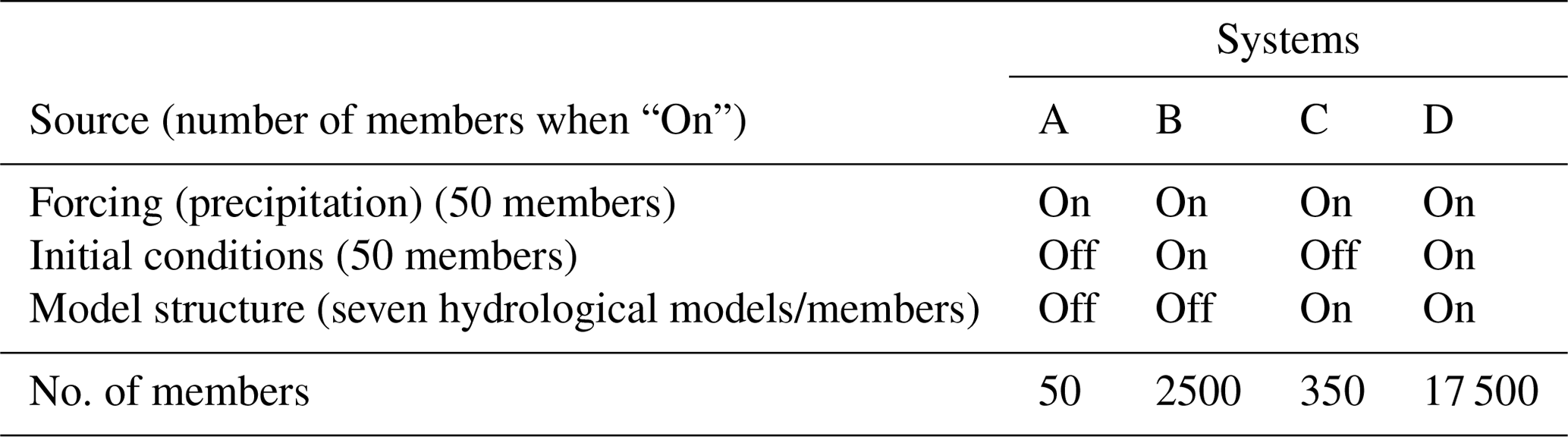
We created four hydrometeorological forecasting systems that differ by how uncertainties are estimated and propagated. They consider the following sources of uncertainty: system A, forcing, system B, forcing and initial conditions, system C, forcing and model structure, and system D, forcing, initial conditions, and model structure. We considered the ECMWF ensemble precipitation forecast over the period 2011–2016 and up to 7 d of forecast horizon, seven hydrological lumped conceptual models, and the ensemble Kalman filter as tools for uncertainty quantification. These three tools represent the forcing, model structure, and initial condition uncertainties, respectively. We investigated their performance across 30 catchments in the province of Quebec (Canada) for each system. Precipitation forecasts are post-processed by applying the censored, shifted gamma distribution proposed by Scheuerer and Hamill (2015).
This paper is structured as follows: Sect. 2 presents the methods, data sets, and case study. Section 3 presents the results, followed by a discussion in Sect. 4 and finally the conclusions in Sect. 5.
2.1 Tools for uncertainty quantification
The ensemble forecasting approach allows us to distinguish the part of uncertainty that comes from different sources. A specific source of uncertainty can be tracked through the modeling chain and along lead times (Boelee et al., 2019). Following Thiboult et al. (2016), we created four ensemble prediction systems that differ in how hydrometeorological uncertainties are quantified (Table 1). Ensembles were built from the HOOPLA (HydrOlOgical Prediction LAboratory; https://github.com/AntoineThiboult/HOOPLA, last access: 23 January 2021) modular framework (Thiboult et al., 2018), an automatic software that allows us to carry out model calibration and obtain hydrological simulations and forecasts at different time steps. They consider uncertainty coming from system A, forcing, system B, forcing and initial conditions, system C, forcing and model structure, and system D, forcing, initial conditions, and model structure. Each source contributes a number of members, from 7 to 50, to the forecasting system when it is turned on, as shown in Table 1. In systems for which hydrological modeling uncertainty is not considered (i.e., A and B), only one model is used, and it is the one presenting median performance during calibration. As shown in Table 1, all systems quantify the forcing (in our case, precipitation) uncertainty. Raw and post-processed ensemble precipitation forecasts drive the hydrological model(s).
In the following sections, we describe each tool that quantifies a different source of uncertainty as applied in this study. We include each technique's conceptual aspects and the reasons behind their selection.
Table 1Forecasting systems A, B, C, and D of the study and total number of members of the resulting ensemble streamflow forecast. On (off) indicates when uncertainty is (is not) quantified with the help of ensemble members.
2.1.1 Precipitation forecast uncertainty: ensemble forecast
Forcing uncertainty is characterized by precipitation ensemble forecasts issued by the European Centre for Medium-Range Weather Forecasts (ECMWF) (Buizza and Palmer, 1995; Buizza et al., 2008), downloaded through the TIGGE database for the 2011–2016 period. In this study, the set consists of 50 exchangeable members issued at 12:00 UTC, for a maximum forecast horizon of 7 d at a 6 h time step.
The database was originally provided with a 0.25∘ spatial resolution and was reduced to 0.1∘ by bilinear interpolation (Gaborit et al., 2013) to ensure that several grid points are situated within each catchment boundary. Additionally, when downscaling, we considered the contribution of the points close to the catchment boundaries, which allows us to have a better description of the meteorological conditions of the catchments and implicitly account for position uncertainty (Thiboult et al., 2016; Scheuerer and Hamill, 2015).
Forecasts and observations were temporally aggregated to a daily time step and spatially averaged to the catchment scale to match the common HOOPLA framework of the hydrological models. In order to isolate the effect of precipitation, observed air temperatures were used instead of the forecast ones. This allows us to focus on changes in streamflow forecast performance attributed only to precipitation post-processing, which is typically the most challenging variable to simulate and the one that mostly impacts hydrological forecasting (Hagedorn et al., 2008).
2.1.2 Precipitation post-processor: censored, shifted gamma distribution (CSGD)
The ECMWF ensemble precipitation forecasts were post-processed over the 2011–2016 period following a simplified variant of the CSGD method proposed by Scheuerer and Hamill (2015). The CSGD is based on a complex heteroscedastic, nonlinear regression model conceived to address the peculiarities of precipitation (e.g., its intermittent and highly skewed nature and its typically large forecast errors). This method yields full predictive probability distributions for precipitation accumulations based on ensemble model output statistics (EMOS) and censored, shifted gamma distributions. We selected the CSGD method because it has broadly outperformed other established post-processing methods, especially in processing intense rainfall events (Scheuerer and Hamill, 2015; Zhang et al., 2017). Moreover, its relative impact on hydrological forecasts has already been assessed at different scales and under various hydroclimatic conditions (Bellier et al., 2017; Scheuerer et al., 2017).
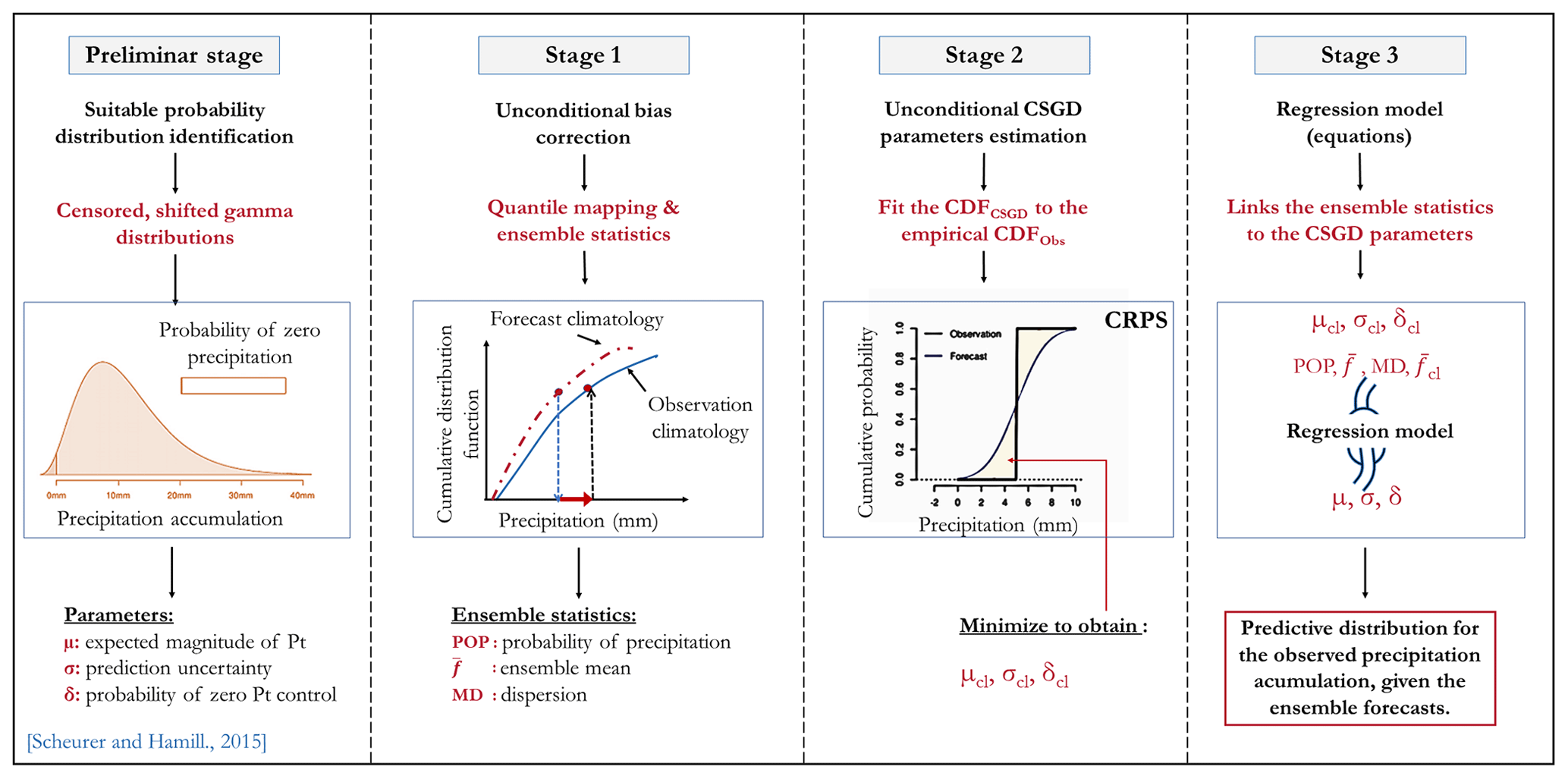
In this study, the original version of the CSGD method was adapted because the ensemble statistics had to be determined on the average catchment rainfall rather than at each grid point within the catchment boundaries. Figure 1 identifies the different stages necessary to apply the method. Briefly, the application of the CSGD was accomplished as follows.
-
Errors in the ensemble forecast climatology were corrected via the quantile mapping (QM) procedure advocated by Scheuerer and Hamill (2015). The QM method adjusts the cumulative distribution function (CDF) of the forecasts onto the observations. In this version, the quantiles were estimated from the empirical CDFs. See Scheuerer and Hamill (2015) for details about the procedure and extrapolations beyond the extremes of the empirical CDFs.
-
The corrected forecasts were condensed into statistics, used as predictors to drive a heteroscedastic regression model. The predictors were the ensemble mean (), the ensemble probability of precipitation (POPf), and the ensemble mean difference (MDf). The latter is a measure of the forecast spread.
-
The CSGD model with mean (μ), standard deviation (σ), and shift (δ; it controls POPf=0) parameters was fitted to the climatological distribution of observations to establish the parameters for the unconditional CSGD (μcl), (σcl), and (δcl). The ensemble statistics from step 1 and the unconditional CSGD parameters were linked to the CSGD model via
where log 1p(x) = log (1+x) and expm1(x) = exp (x)−1. The δ parameter accounts for the probability of zero precipitation. Both the unconditional CSGDs and the regression parameters are fitted by minimizing a closed form of the continuous ranked probability score (CRPS). We refer to Scheuerer and Hamill (2015) for more details about the equations, model structure, and fitting.
Considering that precipitation (and particularly intense events) does not have a temporal autocorrelation (memory) as strong as streamflow (Li et al., 2017), we adopted the standard leave-one-year-out cross-validation approach to estimate the CSGD climatological and regression model parameters. They were fitted for each month and lead time, using a training window of approximately 3 months (all forecast and observations from 90 d around the 15th day of the month under consideration), resulting in a training sample size of 91 × 5 pairs of observations and forecasts.
The CSGD method yields a predictive distribution for each catchment, lead time, and month. This distribution allows one to make a sample and construct an ensemble of any desired size M. As comparing ensembles of different sizes may induce a bias (Buizza and Palmer, 1998; Ferro et al., 2008), we drew ensembles of the same size as the raw forecasts (M=50). Similarly to Scheuerer and Hamill (2015), we sampled the full distribution by choosing the quantiles with level αm = for , which correspond to the optimal sample of the predictive distribution that minimizes the CRPS (Bröcker, 2012).
2.1.3 Reordering method: ensemble copula coupling
EMOS procedures, such as the CSGD method, destroy the spatiotemporal and intervariable correlation of the forecasts. Many studies stressed the importance of correctly reconstructing the dependence structures of weather variables for hydrological ensemble forecasting (Bellier et al., 2017; Scheuerer et al., 2017; Verkade et al., 2013). In this study, we use ensemble copula coupling (ECC) (Schefzik et al., 2013) to address this issue. This technique reconstructs the spatiotemporal correlation by reordering samples from the raw predictive marginal distributions to identify the dependence template. The ECC reasoning lies in the fact that the physical model can adequately represent the covariability between the different dimensions (i.e., space, time, variables). Furthermore, as the template is the raw ensemble, the ECC should have the same number of members as the raw ensemble. Accordingly, the predictive distribution sample with equidistant quantiles with levels αm = is reordered so that the rank order structure is the same as the raw ensemble values. We refer to Schefzik et al. (2013) for more details about the mathematical framework underlying the method.
2.1.4 Initial conditions. Uncertainty: ensemble Kalman filter
The ensemble Kalman filter (Evensen, 2003, EnKF) is used to provide hydrological model states at each time step. The EnKF is a sophisticated sequential and probabilistic data assimilation technique that relies on a Bayesian approach. It estimates the probability density function of model states conditioned by the distribution of observations. In this study, we use the same hyperparameters (EnKF settings) as Thiboult et al. (2016). They were identified after rigorous testing carried out by Thiboult and Anctil (2015) using model performance on reliability and bias as criteria of selection over the same hydrologic region as the present study.
The EnKF performance is highly sensitive to its hyperparameters (Thiboult and Anctil, 2015), which represent the uncertainty around hydrological model inputs and outputs. For precipitation, we used 50 % standard deviation of the mean value with a gamma law. For streamflow and temperature, we used 10 % and 2 ∘C standard deviation with normal distribution, respectively.
At every time step, the EnKF is tuned to optimize reliability and accuracy, per catchment and hydrological model, following two principal stages.
-
Forecasting: N forcing scenarios are propagated using the hyperparameters through the model to generate N members of state variables from the prior estimate of the state (, also called background or predicted state). From this ensemble of state variables, the model's error covariance matrix (Pt, the difference between the true state and the individual hydrological model realizations) is computed and used to calculate the Kalman gain (Kt). Then, the Kalman gain is calculated from Pt and Rt (the covariance of observation noise) according to a weighting coefficient used to update the states of the hydrological model. The Kalman gain is mathematically represented as
where the t indices refer to the time and H is the observation function that relates the state vectors and the observations.
-
Update (analysis): once an observation becomes available (zt), the state variables () are updated as a combination of the prior knowledge of the states (), the Kalman gain (Kt), and the innovation (i.e., the difference between the observed and prior simulated streamflow).
A full description of the EnKF scheme applied in this study is provided in Thiboult and Anctil (2015).
The work of Thiboult and Anctil (2015) demonstrated that EnKF performance is not as sensitive to the number of members as it is to the hyperparameters (at least for the catchments and models used in this study). Ensembles of 25 and 200 members presented similar performances. Therefore, we opted for 50 members as a trade-off between computational cost and stochastic errors when sampling the marginal distributions of the state variables.
2.1.5 Hydrological uncertainty: hydrological models, snow module, and evapotranspiration
To consider model structure and parametrization uncertainties, we use 7 of the 20 lumped conceptual hydrological models available in the HOOPLA framework. Keeping in mind parsimony and diversity as criteria (different contexts, objectives, and structures), Seiller et al. (2012) selected these 20 models, expanding from an initial list established by Perrin (2000).
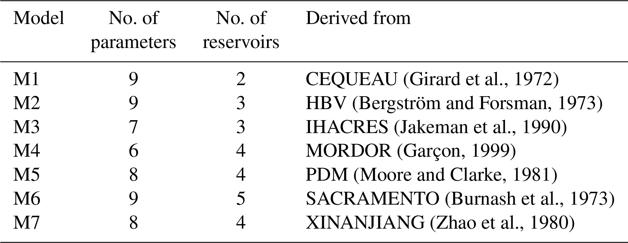
To maximize the benefits from the multimodel approach, with the constraint of low computational time and data management, we opted for seven models with particular attention paid to how they represent flow production, draining, and routing processes. The structures of the selected models vary from six to nine free parameters and from two to five water storage elements. All the hydrological models include a soil moisture accounting storage and at least one routing process. Diversity can be a useful feature for forecasting events beyond the range of responses observed during model calibration (Beven, 2012; Beven and Alcock, 2012) and for catchments that present strong heterogeneities (Kollet et al., 2017). Table 2 summarizes the main characteristics of the lumped models and identifies the original models from which they were derived.
(Girard et al., 1972)(Bergström and Forsman, 1973)(Jakeman et al., 1990)(Garçon, 1999)(Moore and Clarke, 1981)(Burnash et al., 1973)(Zhao et al., 1980)Table 2Main characteristics of the seven lumped models. Modified from Seiller et al. (2012).
All the hydrological models are individually coupled with the CemaNeige snow accounting routine (Valéry et al., 2014). This two-parameter module estimates the amount of water from melting snow based on a degree-day approach. Fed with total precipitation, air temperature, and elevation data, CemaNeige separates the solid precipitation fraction from the liquid fraction and stores it in a conceptual reservoir (snowpack). The model simulates two internal state variables of the snowpack: the thermal inertia of the snowpack Ctg (dimensionless; higher values indicate later snowmelt) and a degree-day melting factor Kf (mm ∘C−1; higher values indicate a faster rate of snowmelt). The latter determines the elapsed melt blade that will be added to the hydrological model. These parameters are optimized for each model.
All the hydrological models were forced with the same input data: daily precipitation and ETP based on a catchment's air temperature and the extraterrestrial radiation (Oudin et al., 2005).
To calibrate the hydrological models, we computed the modified Kling–Gupta efficiency (KGEm) as an objective function (Gupta et al., 2009; Kling et al., 2012) and used the shuffled complex evolution (SCE) as the automatic optimization algorithm (Duan et al., 1994), which is recommended for smaller parameter spaces, as is the case here (Arsenault et al., 2014).
2.2 Case study and hydrometeorological data sets
2.2.1 Study area
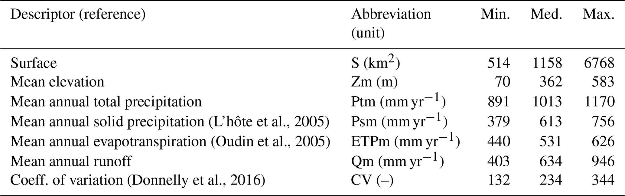
The study is based on a set of 30 Canadian catchments spread over the province of Quebec. These catchments' temporal streamflow patterns are primarily influenced by nivo-pluvial events (snow accumulation, melt, and rainfall dynamics) during spring and pluvial events during spring and fall. The prevailing climate is humid continental, Dfb, according to the Köppen classification (Kottek et al., 2006). Land uses are mainly dominated by mixed woods, coniferous forests, and agricultural lands. Figure 2 displays their location, and Table 3 summarizes physical features and hydrological signatures.
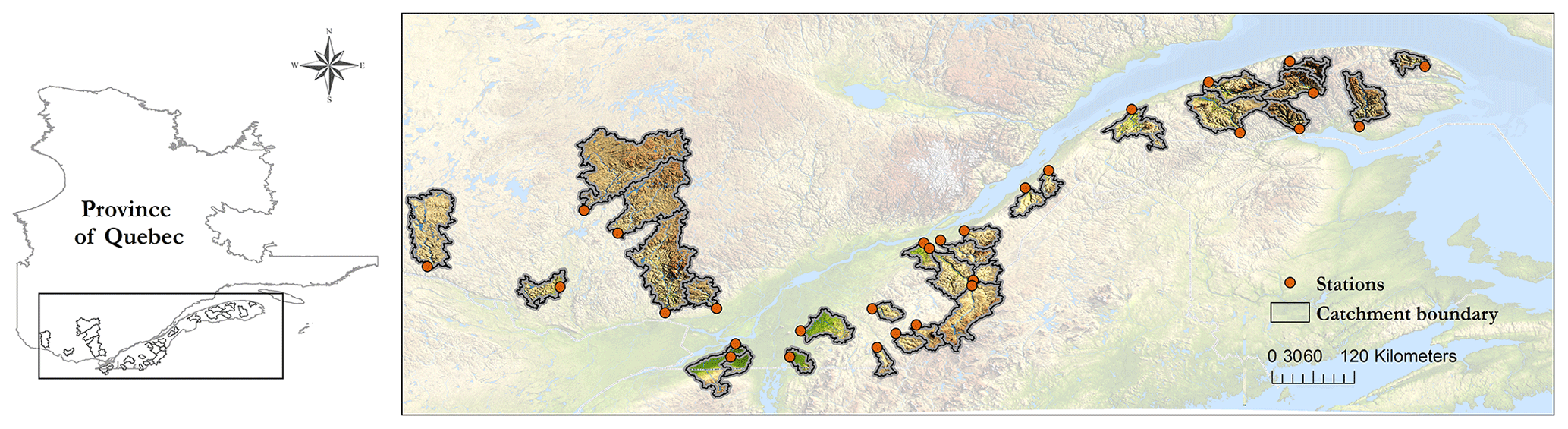
Figure 2Spatial distribution of the 30 studied catchments. Data layers: Direction d'Expertise Hydrique du Québec: catchment boundary, open hydrometric stations, province of Quebec delimitation. Generated by Emixi Valdez, 23 May 2021, using ArcGIS for Desktop Advanced, version 10.4. Redlands, CA: esri, 2015.
Table 3Main characteristics of the 30 catchments. Mean annual values and the coefficient of variation were computed over 1995–2016.
2.2.2 Hydrometeorological observations
The time series of observations extend over 22 years, from January 1995 to December 2016. They were provided by the Direction d’Expertise Hydrique du Québec (DEHQ). They consist of precipitation, minimum and maximum air temperature, and streamflow series at a 3 h time step. Climatological data stem from station-based measurements interpolated on a 0.1∘-resolution grid using ordinary kriging. For temperature, kriging is applied at the sea level using an elevation gradient of −0.005 ∘C m−1. The entire study area is located south of the 50th parallel, considered a region with higher-quality meteorological observations because of the density of the ground-based network (Bergeron, 2016).
Concerning the river discharge series, the DEHQ's hydrometric station network records data continuously, every 15 min, and transmits measurements each hour to an integrated collection system where they are subsequently processed and validated. However, despite constant monitoring and improvements in measurement strategies, these series have missing values during winter since river icing causes a time-varying redefinition of the flow conditions, resulting in highly unreliable measurements. Accordingly, the winter period (December–March) will not be included in the analysis.
In this study, we followed Klemeš (1986) by dividing the available series into two segments: 1997–2007 for calibrating model parameters and 2008–2016 for computing the goodness of fit. The 3 previous years of each period allowed for the spin-up of the models.
2.3 Forecast evaluation
A multi-criteria evaluation is applied to measure different facets contributing to the overall quality of the forecasts. We primarily consider scores commonly used in ensemble forecasting to evaluate accuracy, reliability, sharpness, bias, and overall performance (Brown et al., 2010; Anctil and Ramos, 2019). Verification was conditioned on lead time and catchment size over 2011–2016. To highlight the sensitivity of the results to catchment size, we defined three catchment groups: smaller (<800 km2: 11 catchments), medium (between 800 km2 and 3000 km2: 10 catchments), and larger (≥3000 km2: 9 catchments).
To increase the readability of the text, the equations for each of the selected metrics have been placed in Appendix A. Figure 3 proposes a graphical explanation for some of them.
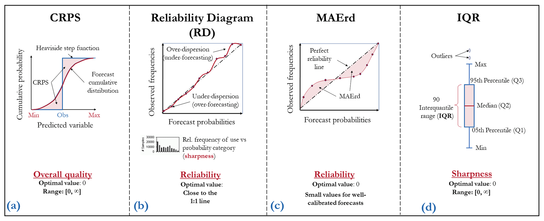
Figure 3Graphical representation of the CRPS, reliability diagram, MAE of the reliability diagram (MAErd), and IQR forecast evaluation criteria.
2.3.1 Evaluation criteria
The relative bias (BIAS) is used to measure the overall unconditional bias (systematic errors) of the forecasts (Anctil and Ramos, 2019). Mathematically, it is defined as the ratio between the mean of the ensemble average and the mean observation. BIAS is sensitive to the direction of errors: values higher (lower) than 1 indicate an overall overestimation (underestimation) of the observed values.
The CRPS is a common metric to measure the overall performance of forecasts (Fig. 3a). It represents the quadratic distance between the CDF of the forecasts and the empirical CDF of the observations (Hersbach, 2000). The CRPS shares the same unit as the predicted variable. A value of 0 indicates a perfect forecast, and there is no upper bound. As the CRPS assesses the forecast for a single time step, the mean continuous ranked probability score (MCRPS) is defined as the average CRPS over the entire evaluation period. We estimate the CRPS from the empirical CDF of forecasts.
Reliability is the alignment between the forecast probabilities and the frequency of observations. It describes the conditional bias related to the forecasts. In this study, it was evaluated using the reliability diagram (Wilks, 2011), a graphical verification tool that plots forecast probabilities against observed event frequencies (Fig. 3b). The range of forecast probabilities is divided into K bins according to the forecast probability (horizontal axis). The sample size in each bin is often included as a histogram. A perfectly reliable system is represented by a 1:1 line, which means that the probability of the forecast is equal to the frequency of the event.
In order to compare the reliability score of precipitation with the reliability score of streamflow forecasts (and for practical purposes and simplification), we use the mean absolute error from the reliability diagram (MAErd, Fig. 3c). In this case, the MAErd measures the distance between the predicted reliability curve and the diagonal (perfect reliability). To compute the MAErd, we calculate nine confidence intervals with a nominal confidence level of 10 %–90 %, with an increment of 10 % for each emitted forecast. Then, it was established whether or not each confidence interval covered the observation for each forecast and each confidence interval. In a well-calibrated distribution, the observation inside each confidence interval and its corresponding nominal confidence level should be close, taking the form of a linear relationship of 1:1 (as the reliability diagram).
To see the performance of the post-processor conditioned to precipitation amount, we decided to use the reliability diagram to evaluate the reliability of the forecast probability of precipitation for thresholds of different exceedance probabilities (EPs) in the sampled climatological probability distribution, namely, 0.05, 0.5, 0.75, and 0.95. We turn the ensemble forecast into binary predictions that have the value 1 if the precipitation amount exceeds the thresholds based on these quantiles and 0 otherwise.
To measure the degree of variability of the forecasts or the sharpness of the ensemble forecasts, we use the 90 % interquantile range (IQR). It is defined as the difference between the 95th and 5th percentiles of the forecast distribution (Fig. 3d). The narrower the IQR, the sharper the ensemble. As the sharpness is a property of the unconditional distribution of forecasts only (sharp forecasts are not necessarily accurate or reliable; sharp forecasts are accurate if they are also reliable), we use this attribute as a complement to the reliability (i.e., given two reliable systems, sharper is better) (Gneiting et al., 2007). The frequency of forecasts shown in the reliability histogram (Fig. 3b) gives information on sample size and sharpness as well. A sharp forecast tends to predict probabilities near 0 or 1.
2.3.2 Skill scores
Skill scores (SSs) are used to evaluate the performance of a forecast system against the performance of a reference forecast. The criteria described in Sect. 2.3.1 can be transformed into a SS by using the relationship described in Eq. (6):
where SScoreSyst and SScoreRef are the scores of the forecasting system and the reference, respectively. The SS values range from −∞ to 1. If SS is superior (inferior) to 0, the forecast performs better (worse) than the reference. When it is equal to 0, both systems have the same performance or skill.
Since our goal is to determine the value added by a precipitation post-processor in the quantification of streamflow forecasting uncertainty, we use the raw forecasts as a benchmark (Pappenberger et al., 2015).
Results are presented in three subsections. In Sect. 3.1, we present the performance of the raw and post-processed precipitation forecasts. In Sect. 3.2, we discuss the performance of the raw and post-processed streamflow forecasts and the contribution to the performance of the sources of uncertainty considered in each forecasting system analyzed, highlighting the interactions with the precipitation post-processor. Finally, the performance of the precipitation post-processor conditioned to catchment size is presented in Sect. 3.3.
3.1 Ensemble precipitation forecasts
This section assesses and compares the quality of the raw (blue) and post-processed (red) precipitation forecasts (average precipitation over the catchments). Values presented are average daily scores over the evaluation period (2011–2016). Verification metrics for the ensemble precipitation forecasts are shown in Figs. 4 and 5. Figure 4 presents BIAS, MCRPS, MAErd, and IQR scores as a function of lead time. Each box plot combines values from all the catchments. Figure 5 shows the reliability diagrams for the probability of precipitation forecasts exceeding the 0.05, 0.5, 0.75, and 0.95 quantiles for lead times 1, 3, and 6 d. The confidence bounds shown in the curves result from a bootstrap with 1000 random samples representing the 90 % confidence interval. The curves represent the median curve of the 30 catchments. The inset histograms depict the frequency with which each probability was issued. Values supporting the qualitative analysis represent the mean of the catchments.
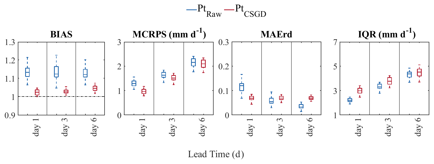
Figure 4BIAS, MCRPS, MAErd, and IQR of raw (blue) and post-processed (red) daily catchment-based precipitation forecasts for lead times of 1, 3, and 6 d over the evaluation period (2011–2016). Box plots represent the distribution of the scores over 30 catchments.
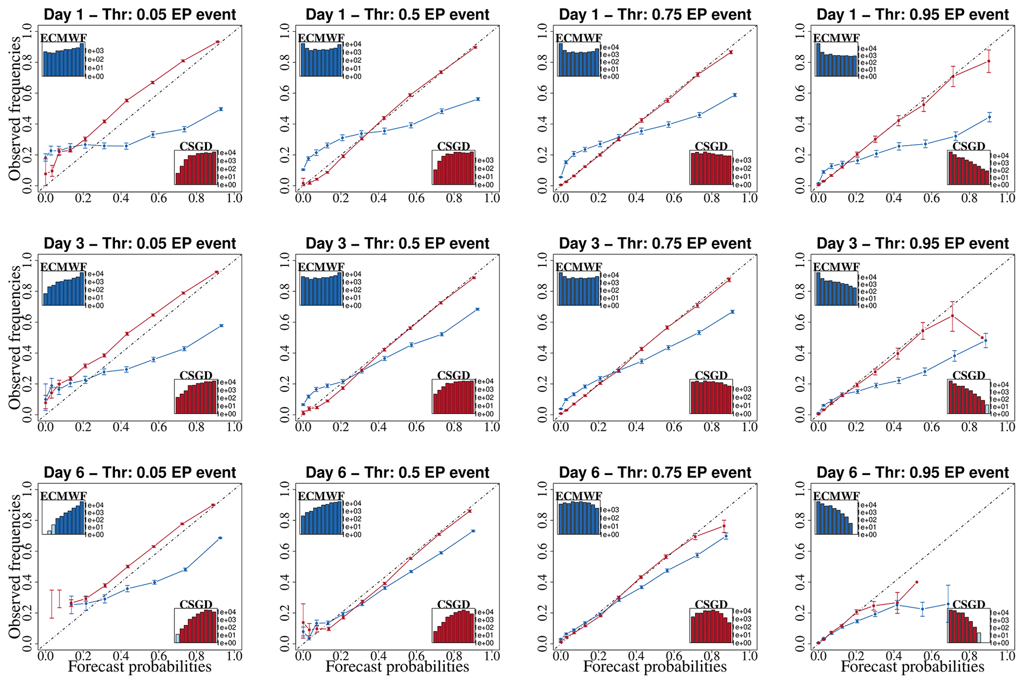
Figure 5Reliability diagrams of raw (blue) and CSDG post-processed (red) precipitation forecasts for lead times of 1, 3, and 6 d and different exceedance probability (EP) thresholds (, and 0.95 quantile of observations), calculated over the evaluation period (2011–2016). The lines correspond to the median curve of all 30 catchments. The bars indicate 90 % confidence intervals of observed frequencies from bootstrap resampling. The inset histograms depict the frequencies with which the category was issued.
3.1.1 Performance of raw precipitation forecasts
As expected, the quality of the raw forecasts generally decreases with increasing lead times. BIAS values range on average from 1.13 to 1.12 for lead times 1 and 6 d, respectively, indicating that the precipitation forecasts overestimate the observations. The MCRPS shows that the overall forecast quality decreases with lead time (from 1.29 to 2.14) while reliability improves (from 0.13 to 0.06), as revealed by the reliability diagram mean absolute error (MAErd). This is a general characteristic of weather forecasting systems, as the dispersion of members increases with the forecast horizon to capture increased forecast errors. Reliability improvement is reflected in BIAS, where a slight decrease in the overestimation is observed as the lead time increases. The typical trade-off between reliability and sharpness is also illustrated (the MAErd vs. IQR). IQR has an opposite behavior to the MAErd, indicating a less sharp forecast with increased lead time.
Regarding the reliability diagram, raw precipitation forecasts tend to under-forecast the low probabilities and over-forecast the high ones. Similarly, as shown in Fig. 4, raw precipitation reliability increases with lead time except for large precipitation amounts (0.95 EP event).
3.1.2 Performance of corrected precipitation forecasts
As illustrated in Fig. 4, the CSGD post-processor substantially reduces the relative bias of the meteorological forecasts since day 1, and its effectiveness is maintained over time and for all catchments. The BIAS of the post-processed precipitation forecasts ranges from 1.02 to 1.04 for lead times 1 and 6 d, respectively. When considering MCRPS, the performance of the CSGD post-processor decreases when increasing lead times. For example, at lead times 1 and 6 d, the MCRPS equals 1.29 and 2.14, respectively. This result is expected as the predictors use information from the raw forecasts (Scheuerer and Hamill, 2015), which also decreases in MCRPS quality with lead time.
In terms of MAErd, the post-processed and raw forecasts have an inverse behavior: while reliability increases rapidly with lead time for raw forecasts, it slightly decreases for post-processed forecasts. CSGD MAErd values range from 0.04 to 0.07 for lead times 1 and 6 d, respectively. On the other hand, the post-processor was unable to consistently improve the precipitation ensemble's reliability and sharpness. Rather, in contrast to the raw ensemble, the IQR increases regardless of whether precipitation reliability improves or not. However, on day 6, we note that raw forecasts are more reliable on median values over the catchments while also being sharper than post-processed forecasts.
The reliability diagram confirms the results in Fig. 4. In general, the performance of the CSDG post-processor in terms of reliability decreases with increasing lead times and precipitation thresholds. The CSGD post-processed precipitation forecasts are already reliable at short lead times (1 d) except for the EP event of 0.05, which in fact corresponds closely to the probability threshold of zero precipitation. The CSGD post-processor tends to generate forecasts that underestimate the observations for this threshold, although this trend decreases as lead time increases. This can be attributed to the fact that the CSGD post-processor retains the climatological shift parameter (δ=δcl) that tends to produce a bias in POPf estimates (Ghazvinian et al., 2020). Moreover, in both cases (raw and post-processed), the more reliable the forecast, the flatter the histogram. This indicates that the forecasts predict all probability ranges with the same frequency, and therefore the system is not sharp (a perfectly sharp system populates only 0 % and 100 %).
3.2 Ensemble streamflow forecasts
This section assesses the quality of the raw streamflow forecasts (blue) and the contribution of the precipitation post-processor (red) to forecast performance from quantifying different sources of uncertainty. Scores are presented for days 1, 3, and 6 in box plots representing all catchments. Figures 6 and 7 illustrate the main interactions of the precipitation post-processor with the hydrological forecasting systems. As summarized in Table 1, systems are ordered from the simplest (A: one source of uncertainty) to most complex (D: three sources of uncertainty). Values supporting the qualitative analysis represent the mean of the catchments.
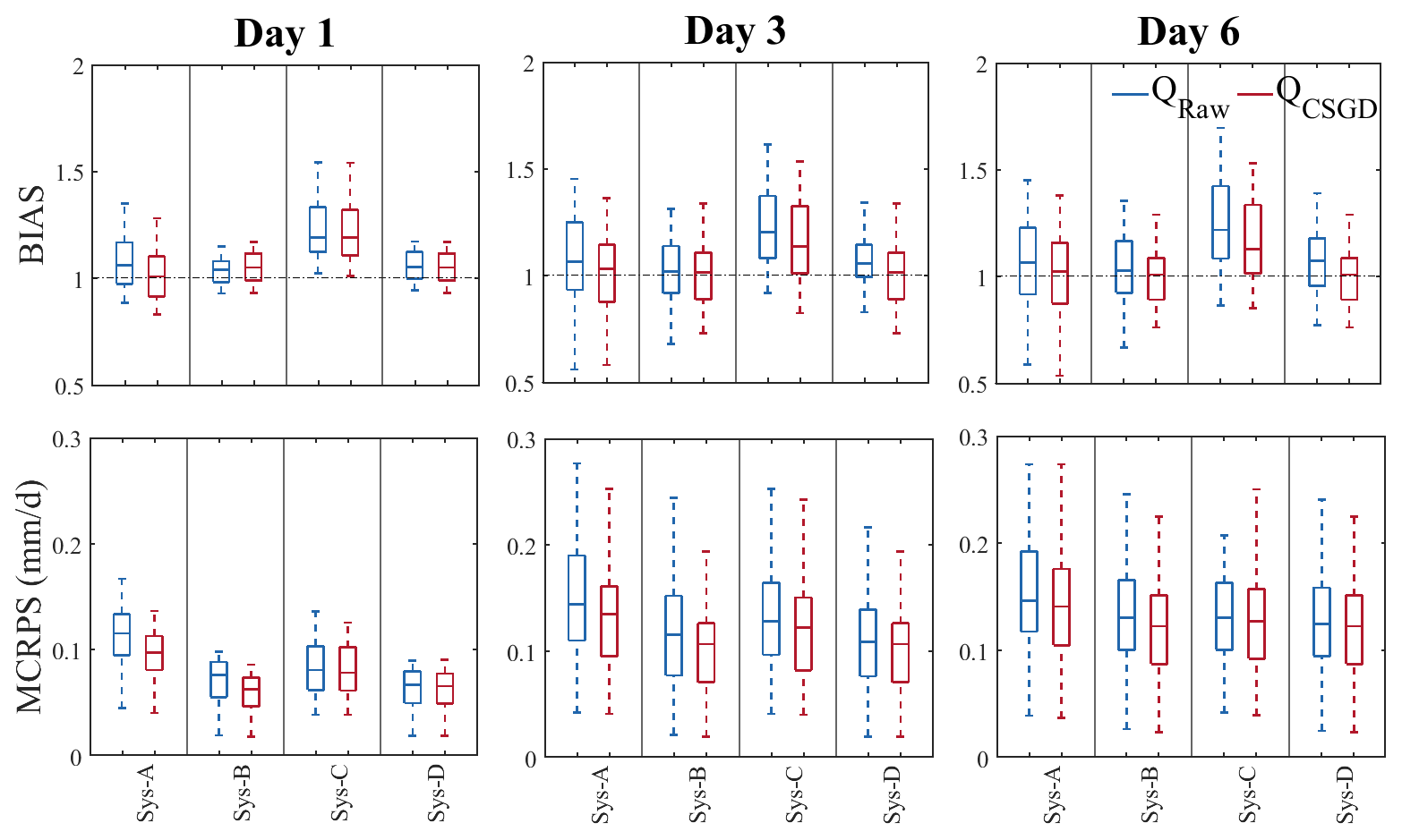
Figure 6Relative bias (BIAS) and MCRPS of the ensemble streamflow forecasts of the four hydrological prediction systems and lead times 1, 3, and 6 d when considering raw (blue) and post-processed (red) precipitation forecasts. Box plots represent the score variability over the 30 catchments.
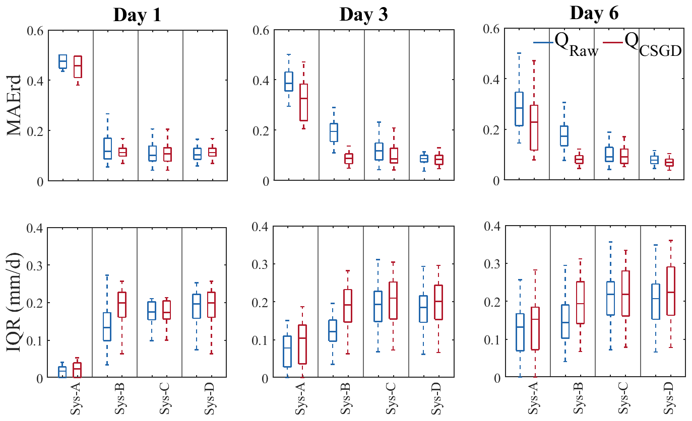
Figure 7MAE of the reliability diagram (MAErd) and interquantile range (IQR) of the ensemble streamflow forecasts of the four hydrological prediction systems and lead times 1, 3, and 6 d when considering raw (blue) and post-processed (red) precipitation forecasts. Box plots represent the score variability over the 30 catchments.
3.2.1 Performance of raw streamflow forecasts
BIAS indicates that systems B and C present the highest and lowest performances, respectively (Fig. 6, BIAS; blue box plots). For system B, BIAS values range on average from 1.04 to 1.03 for lead times 1 and 6 d, respectively. These values are 1.23 and 1.25 for system C. In fact, the systems that benefit from EnKF (i.e., B and D) show better performance, especially at the first lead times. For example, the BIAS values for system D increase from 1.05 to 1.06 for lead times 1 and 6 d, respectively. As the EnKF DA updates the hydrological model states only once (when the forecast is issued), its effects fade out over time. This explains why systems A and B tend to behave similarly as lead time increases. In the case of system A, the BIAS values decrease from 1.08 to 1.07 for lead times 1 and 6 d, respectively. This behavior is inherited from the precipitation forecast as explained in Sect. 3.1.1. System C, which exploits multiple models, overestimates the observations in most catchments, especially at the first lead time. This behavior is inherited from the hydrological models (see the Supplement). This behavior is not penalized as much in systems with a single model since they use the median during calibration. Although at first glance this seems like a better alternative, it is not realistic. In practice, it is difficult to predict which model will be the best predictor on any given day and basin. The BIAS evaluation also reveals that catchment diversity is one factor explaining differences in performance. As lead time increases, forecasts tend to underestimate the observations for some catchments.
As in BIAS, systems B and D are the ones that present the best MCRPS (Fig. 6, MCRPS; blue box plots). The values for the four systems range from 0.12, 0.08, 0.09, and 0.07 at lead time 1 d to 0.15, 0.14, 0.14, and 0.13 at lead time 6 d, respectively. The improvement brought by systems B and D could be attributed to the fact that these are the two systems with the largest number of members. Studies have shown that sample size influences the computation of some criteria, such as the CRPS (Ferro et al., 2008). However, Figs. 6 and 7 show that the effect of the quantification of uncertainty sources is more critical than the ensemble size since systems B, C, and D present a similar range of score when the contribution of EnKF is minimal (i.e., on day 6). These results are in agreement with those found by Thiboult et al. (2016) and Bourgin et al. (2014), who suggested that short-range forecasts benefit most from data assimilation. From Fig. 6 we can also see that system A presents the most unfavorable scenario, which is expected since it only carries meteorological forcing uncertainty with it, and the accuracy of weather forecasts tends to decrease with lead time (Fig. 4, MCRPS; blue box plots).
The MAErd and IQR, together, allow us to evaluate the contribution of each tool to uncertainty quantification in terms of their ability to capture the total uncertainty over time. The MAErd shows that system A follows a pattern similar to the weather forecasts (Fig. 4, MAErd), becoming more reliable with increasing lead times (their values range from 0.47 to 0.29 for lead times 1 and 6 d, respectively) but less sharp (values of IQR from 0.02 to 0.13). In general, when a system has an under-dispersion, it is sharper but unreliable.
System B loses reliability on day 3 (from 0.14 to 0.20) because the EnKF effects fade out over time. However, it becomes slightly more reliable on day 6 (from 0.20 to 0.18) because of the spread of the precipitation forecasts. This is also the case with system C, which also benefits from the meteorological ensemble. Unlike system B, its performance remains almost constant (∼0.11) over time, thanks to the hydrological multimodel. System D is less reliable on day 1. According to Thiboult et al. (2016), the combination of EnKF and the multimodel ensemble causes an over-dispersion since the EnKF indirectly quantifies uncertainty from the hydrological model structure and its parameters when performing DA with the estimation of initial condition uncertainty. Nevertheless, forecast over-dispersion is reduced as the EnKF effects vanish with lead time, and the system becomes more reliable on day 6 (MAErd values = 0.11, 0.08, and 0.07 for lead times 1, 3, and 6 d, respectively). Although the EnKF loses its effectiveness over time, the difference between systems C and D on day 6 reveals that its contribution to forecast performance is still important at longer lead times.
3.2.2 Interaction of the precipitation post-processor with the hydrological forecasting systems
In terms of BIAS (Fig. 6, BIAS; red box plots), we observe that post-processing precipitation forecasts has a much higher impact on the quality of precipitation forecasts (Fig. 4, BIAS; red box plots) over time than on the quality of streamflow forecasts. For example, the percentage improvement over the lead times in precipitation was 8.83 %, while the system with the greatest improvement (system A) was 5.11 %. On day 1, the CSGD post-processor does not have much effect on streamflow forecasts, except for system A, which is a system that depends exclusively on the ability of the ensemble precipitation forecasts to quantify forecast uncertainty. Even on the first day, the post-processor has a negative effect on system B, reducing its performance by 1.66 %, while systems C and D were improved by less than 1 %. However, these systems were improved by a higher percentage (6.13 % and 6.27 %, respectively) than systems A and B (4.87 % and 3.39 %, respectively) at the furthest lead times.
Additionally, the increased bias on days 3 and 6 in system A reveals that at these lead times forcing uncertainty does not represent the dominant source of uncertainty for some catchments. This implies that a simple chain with a precipitation post-processor may be insufficient to systematically provide unbiased hydrological forecast systems. At these lead times, in terms of BIAS, the performance of raw forecasts in systems B and D are generally similar to the performance of post-processed forecasts in system A. System C, which has the lowest performance, is also improved by the precipitation post-processor. However, this improvement still shows the worst performance (average BIAS = 1.18) compared to the other systems based on raw precipitation forecasts (average BIAS: A = 1.08, B = 1.03, and D = 1.06).
In terms of overall quality (MCRPS), the streamflow forecasts based on post-processed precipitation forecasts perform better for systems A and B, but only at the shorter lead times (Fig. 6, MCRPS). These systems improved by 13.91 % and 18.83 %, respectively, on day 1. In the longer lead times, the effect of the CSDG post-processor is reduced. For system A, the improvements fluctuate between 7.78 % and 6.11 % for lead times 3 and 6 d, respectively. These values are equal to 12.80 % and 10.06 % for system B. Systems C and D, on the other hand, appear to be unaffected by the post-processing of precipitation forecasts at the short lead times and slightly improved by the post-processor with increasing time. For system C, the improvements range from 2.12 % to 5.92 % for lead times 1 and 6 d, respectively, while for system D, these values are equal to 1.17 % and 3.46 %.
We also observe that the performance of raw forecasts in all systems, notably in systems B (average MCRPS = 0.11) and D (average MCRPS = 0.10), is generally better than post-processed forecasts in system A (average MCRPS = 0.13). Furthermore, differences are higher at shorter lead times and tend to decrease at longer lead times. This indicates that benefits are brought by quantifying more sources of uncertainty, especially at shorter lead times, instead of just relying on forcing uncertainty quantification through post-processed ensemble precipitation forecasts to enhance the overall performance of ensemble streamflow forecasting systems.
In terms of reliability (Fig. 7, MAErd), systems that use a single hydrological model (A and B) are the ones that benefit the most from post-processing precipitation forecasts. When a multimodel approach is used (C and D), the system becomes more robust, and differences in streamflow forecast quality from using or not a precipitation post-processor are small. The improvements of the four systems on day 1 are equal to 4.83 %, 19.7 %, 0.28 % and −6.43 %. On day 6, these values are 20.79 %, 55.20 %, 9.20 % and 9.46 %. These values suggest that the contribution of the CSGD precipitation post-processor is more important for system B (i.e., the post-processor has better interaction with the DA EnKF). The underlying reason for this is associated with the fact that the CSGD over-dispersion (Fig. 5, first column) compensates for the loss of dispersion from the use of EnKF DA, in contrast to system D, which is already over-dispersed. The reliability of system B decreased by 6.43 % on the first day with the post-processor.
It is interesting to note that, for systems B, C, and D, streamflow forecasts based on raw precipitation forecasts are always much better (average MAErd=0.17, 0.11, and 0.09, respectively) than streamflow forecasts based on post-processed precipitation forecasts in system A (average MAErd=0.32). Similarly to the bias and the overall performance, this indicates that forcing uncertainty only is not enough to deliver reliable streamflow forecasts, and quantifying other sources of hydrological uncertainty can be more efficient than only post-processing precipitation forecasts.
For the IQR (Fig. 7, IQR), we again see a trade-off with reliability. The increased dispersion that contributes to the reliability of the systems makes the forecasts less sharp. For example, system B, which shows the greatest benefit from the precipitation post-processing in terms of reliability, is also the one that is less sharp when compared to its raw forecast counterpart. Finally, although post-processed systems C and D display similar reliability scores, the more complex system does not display sharper forecasts. The gain in the system's complexity does not translate into an important gain in reliability/sharpness of the forecasts.
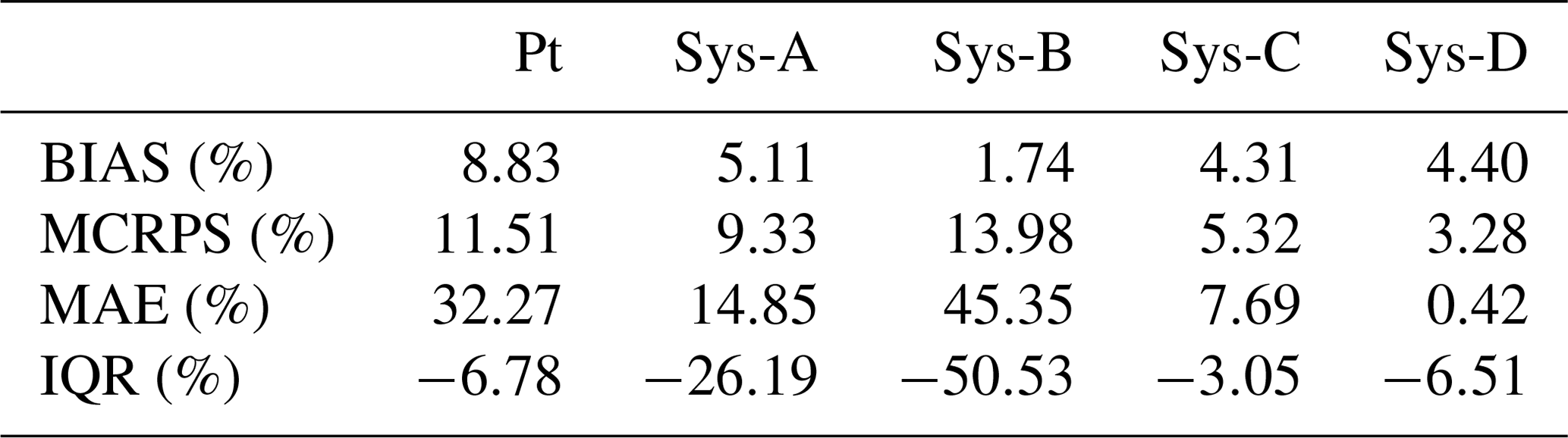
Table 4 summarizes the percentage of performance improvement (positive values) or deterioration (negative values) brought by the precipitation post-processor according to each criterion of forecast quality (BIAS, MCRPS, MAErd, IQR) when evaluating precipitation (Pt) and streamflow (Sys-A to Sys-D) forecasts.
Table 4Percentage of performance improvement (positive values) or deterioration (negative values) brought by the precipitation post-processor according to each criterion of forecast quality (BIAS, MCRPS, MAErd, IQR) when evaluating precipitation (Pt) and streamflow (Sys-A to Sys-D) forecasts.
3.3 Effect of catchment size
Figure 8 shows the MAErd of the median results of the catchments analyzed according to three groups (smaller, medium, and larger) and for the 7 d of lead time. The first column corresponds to the MAErd of precipitation forecasts and the rest to the MAErd of streamflow forecasts issued by the four hydrological prediction systems. In general, the performance of precipitation and streamflow forecasts increases with catchment size. This is particularly observed in the streamflow forecasts and may be related to the fact that larger catchments tend to experience lower streamflow variability (Sivapalan, 2003), and it is thus easier for the hydrological models to simulate their streamflows (Andréassian et al., 2004). Moreover, weather can differ substantially over a couple of kilometers, and the resolution of NWP models is often too coarse to capture these variations in smaller catchments. For example, extreme localized events can be missed in small catchments if the amount of precipitation is well predicted but in the wrong location. In larger catchments, a buffer effect can be generated, and displacements of precipitation may impact less the predictions of streamflow.
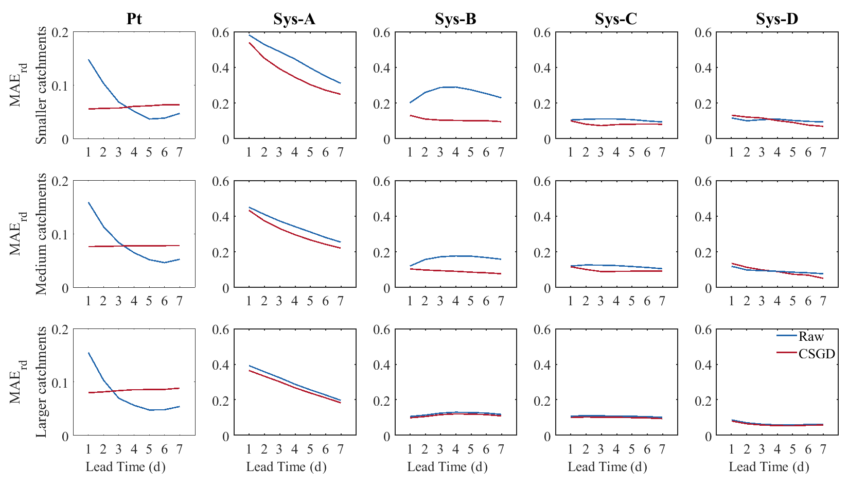
Figure 8MAErd for raw (blue) and precipitation post-processed (red) forecasts for precipitation (Pt) and streamflow forecasts as a function of forecast lead time. The first column represents the MAErd for the raw and post-processed precipitation forecasts. The remaining columns represent the four streamflow forecasting systems (A, B, C, and D). On top: the smaller catchment group. In the middle: the medium catchment group. On the bottom: the larger catchment group.
The effect of post-processing on precipitation forecasts remains practically constant over time, independently of the catchment size. Improvements from precipitation post-processing are greatest on the first 3 d for the three catchment groups. From day 4 onwards, the raw forecast becomes more reliable. When evaluating the streamflow forecasts, the groups that benefited most from the post-processor were those with the smaller- and medium-sized catchments (Fig. 8, top and middle panels). The effect of the precipitation post-processor for the group with the larger catchments is practically negligible, as we can see in Fig. 8, bottom panel, as the red and blue curves are superposed.
Concerning the systems, the most benefited are systems A and B, in contrast to systems C and D, whose improvements are reflected in the most distant lead times, corroborating the results obtained in Sect. 3.2. The gain in streamflow in the last few days comes from the fact that the CSGD compensates for the loss of dispersion of the systems in the last few lead times. This dispersion is not beneficial to the raw precipitation, as it increases with time. This explains why even though the raw precipitation is more reliable in the late lead times, the post-processor still generates gains in streamflow forecast performance.
The evolution of the MAErd of the raw forecasts illustrates the contribution of each of the tools used to quantify forecast uncertainty in the systems. For example, in system A, MAErd inherits the patterns of the meteorological forecasts: it becomes more reliable with increasing lead time. For system B, we see the contribution of EnKF DA for the first lead time and the decrease in performance until day 4, when the contribution from the spread of the precipitation ensemble forecast becomes dominant over the reduction of uncertainty from the DA and the hydrological forecasts start to spread again. In system C, the MAErd decreases with regard to the MAErd of systems A and B, and it remains constant over time, confirming that the multimodel is the source that contributes the most to the reliability of the ensemble streamflow forecasts. Finally, the results for system D show a peak of high spread on day 1. This over-dispersion is generated by combining the multimodel and the EnkF DA.
3.3.1 Gain in streamflow forecasts from the CSGD post-processing
Figure 9 presents the MCRPS skill scores of precipitation forecasts (Pt-MCRPS SS) against the skill scores of streamflow forecasts (Q-MCRPS SS) after application of the CSGD post-processor to the raw precipitation forecasts. The skill scores are computed using the raw forecasts as a reference. The results are presented for the three catchment groups and lead times 1, 3, and 6 d.
Figure 9 shows that, overall, improvements in precipitation forecasts are mostly associated with improvements in streamflow forecasts (points located in quadrant I; top right). In a few cases (Sys-B day 1; Sys-C and Sys-D days 3 and 6), however, improvements in precipitation forecasts are associated with negative gains in streamflow forecasts (points located in quadrant II; top left). In some cases, improvements in precipitation are negligible but streamflow forecasts deteriorate. These cases are mainly observed in smaller catchments, in longer lead times (day 6), and for the systems that include hydrological model structure uncertainty (Sys-C and Sys-D).
Figure 9 also reveals how the different forecasting systems interact with the precipitation post-processor to improve or deteriorate the performance of the streamflow forecasts. For example, on day 3, considering system A (Sys-A), the gain in precipitation for a catchment pertaining to the group of smaller catchments (blue circle in the red square) does not impact the skill score of the streamflow forecasts. However, when activating the EnKF DA (e.g., Sys-B), the streamflow forecast performance of the same catchment is improved. This improvement remains when evaluating system C and system D, although the skill score is lower (the example is indicated with red arrows in the figure). This illustrates the fact that the effect of a precipitation post-processor can be amplified when combined with the quantification of other sources of hydrological uncertainty.
A clear pattern related to catchment size is not evident, although smaller- to medium-sized catchments seem to display higher skill scores for streamflow forecasts.
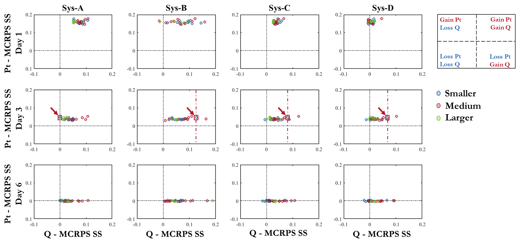
Figure 9MCRPS skill score of precipitation forecasts against the MCRPS skill score of streamflow forecasts after application of the CSGD precipitation post-processor. The skill scores are computed using raw forecasts as a reference. Results are shown for lead times of 1, 3, and 6 d and catchment group. The red box and arrows in the middle panels highlight the interaction of the precipitation post-processor with the different sources of uncertainty for the same catchment.
In this section, we discuss the questions of this study. Is precipitation post-processing needed in order to improve streamflow forecasts when dealing with a forecasting system that fully or partially quantifies many sources of uncertainty? How does the performance of different uncertainty quantification tools compare? Finally, how does each uncertainty quantification tool contribute to improving streamflow forecast performance across different lead times and catchment sizes?
Although the precipitation post-processor undeniably improves the quality of precipitation forecasts (Figs. 4 and 5), our results suggest that a modeling system that only tackles the quantification of forcing (precipitation) uncertainties (in our case, system A) with a precipitation post-processor is insufficient to produce reliable and accurate streamflow forecasts (Figs. 6–8). For example, in terms of bias, the improvement brought by the post-processor to the worst-performing systems (systems A and C) did not outperform the other systems based on the raw precipitation forecasts. Interestingly, our study also shows that considering a post-processor while quantifying all sources of uncertainty does not always lead to the best results in terms of streamflow forecast performance either (e.g., Fig. 8, system D), at least with the tools used in this study. With an in-depth analysis of various configurations of forecasting systems, our study confirms previous findings indicating that precipitation improvements do not propagate linearly and proportionally to streamflow forecasts. Although all systems benefit from precipitation post-processing, improvements are conditioned to many factors, the most important being (of those evaluated in this study) system configuration, catchment size, and forecast quality attribute.
The performance of the systems exploiting a multimodel (systems C and D) was less improved by the post-processor than the systems with DA and ensemble precipitation alone (systems A and B), notably for the first few days of lead times. However, the degree of improvement depends on the attribute evaluated. For example, systems A and B improved overall quality by 5.11 % and 1.74 %, respectively. In contrast, the percentages in reliability were 14.85 % and 45.35 %, representing a substantial difference with systems C and D (improved by 7.69 % and 0.42 %, respectively) (see Table 4). Several reasons can explain these differences. For example, the CSGD post-processor has a strong effect on the ensemble spread and tends toward over-dispersion. In systems where the ensembles are more dispersed than needed (e.g., system D), this specific combination produces a greater over-dispersion that affects the system's reliability. As shown in Fig. 7, the multimodel approach was the main contributor to increasing ensemble spread over lead time. In contrast, DA has a lesser effect on the spread of the ensemble members. The application of a DA procedure has more impact on the biases of the ensemble mean. This explains why, when post-processing is not applied to precipitation forecasts, systems endowed with DA present the lowest bias and the best overall performance and multimodel systems present the best reliability.
Table 5 summarized under which circumstances a simple system with a precipitation post-processor may be a better option than to quantify all (or at least the most important) known sources of uncertainty. It shows, for instance, that a user interested in better CRPS performance at longer lead times (here, day 6) should look forward to implementing a forecasting system that considers DA and a post-processing (Sys-B + CSGD). Combined with precipitation post-processing, less complex systems can be good alternatives, such as those considering forcing and initial condition uncertainty (Figs. 6 and 7, system B) and those considering forcing and multimodel uncertainty (Fig. 8, system C). If the priority is to achieve a reliable and accurate system, then system B with precipitation post-processor presents a better alternative than a system like D. This is important since current operational systems are often similar to systems B and C because they are less computationally demanding and more prone to producing information in a timely fashion. For example, for a potential end-user that seeks a fast system to explore policy actions in a very short term, system D is not appropriate.
Table 5Synthesis of the best options available for a forecast user when partial uncertainty quantification systems (A, B, and C) with a precipitation post-processor are compared against a full uncertainty quantification system D without a post-processor in terms of BIAS, overall quality, and reliability for days 1 and 6.
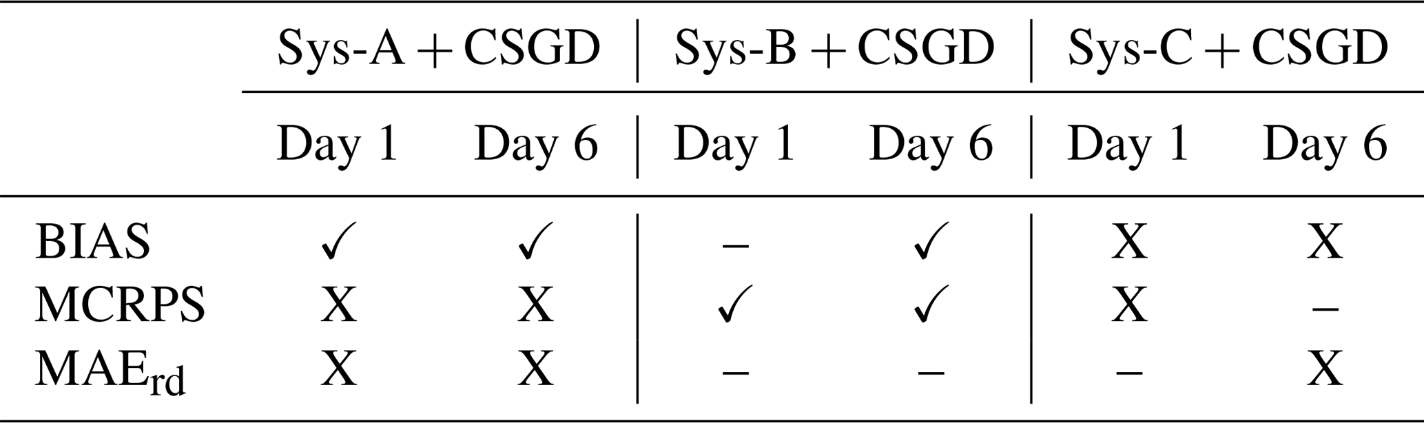
(✓): simple systems with post-processor outperform raw-system D. (X): simple systems with post-processor do not outperform raw-system D. (–): simple systems with post-processor have similar performance to raw-system D.
Although post-processing techniques in hydrology are quite mature, there are still some ambiguities as to how to use them and under which circumstances their application is most operationally advantageous. Based on our results, we cannot give a definitive answer if the precipitation post-processor is a mandatory step or not. However, under similar conditions to those studied here, there has been an indication that precipitation post-processing may be skipped when (1) the hydrological uncertainty is dominant and (2) its drawbacks are relevant for the end-user. In the first case, the improvements brought by the post-processor could not offset the hydrological errors and may even amplify them (e.g., systems C and D). Another example is in large basins, where the precipitation error is smaller and the errors of initial conditions are more significant. The second case is probably worth a whole discussion on its own. For example, the results of statistical post-processors are usually probability distributions that are disconnected in time and space. If the decisions depend on precipitation forecasts that must be very coherent (coherent traces in time and space), it is better to put efforts into a streamflow post-processor or in another component of the forecasting chain because the loss of space–time coherency brought by statistical precipitation post-processors is likely to generate a different response from the catchment (faster/slower flood and event duration, for instance). The need to apply, after the statistical post-processing, an effective reordering technique to retrieve coherent ensemble traces will then be crucial. Another situation is when a drawback is amplified by another component such as when the post-processor has tendencies to over-dispersion and is used in a system that is already over-dispersed. Another situation, not studied here, is when the effect of the post-processor is already accounted for by another element in the hydrometeorological forecasting chain. It is not worth the effort to apply a precipitation post-processor if a hydrological uncertainty processor that lumps all sources of uncertainty will be applied later.
The activation of post-processing and the system's component selection also depends on the most important features of the forecasting chain envisaged by the end-user. Likely the improvements experienced in a system such as D and the implementation of a complex and sophisticated correction technique will not be justified due to the time and computational and human resources that such improvements demand. Although syntheses of benchmarking performance studies can be helpful for deciding on investments, at least when resources are scarce, knowing the minimum percentage of improvement required of the post-processor for decision-making is also a crucial factor. From our study, for instance, in the hypothetical case that a system needs to improve BIAS by more than 10 %, applying a post-processor would not be sufficient (Table 4).
Concerning catchment size, the groups that benefited most from the post-processor were the ones with the smaller- and medium-sized catchments. In the case of the larger catchments, the effect was almost negligible. NWP forecasts of precipitation are usually more uncertain in small domains, where precipitation forcing is also generally the most dominant source of uncertainty. This means that the use of a conditional bias correction, such as the CSGD post-processor used here, based on predictors that can represent well the catchment's characteristics, becomes crucial. Missed or underestimated extreme precipitation events have a more critical impact on small catchments than on large ones, which typically present a more area-integrated hydrological response. Larger catchments generally have greater variability over their drainage area, so uncertainties associated with initial conditions may be more dominant than uncertainties associated with precipitation, and, therefore, the inclusion of the DA component in the forecasting chain might play a more critical role.
Finally, selection and implementation of techniques to quantify different sources of uncertainty have a larger impact on forecast performance over time than the ensemble size. Most studies conclude that increasing the ensemble size improves performance (Ferro et al., 2008; Buizza and Palmer, 1998) and may generate biases when comparing systems with different ensemble sizes. However, that was not always the case in our study. System B, with 2500 members, performed similarly to system C (350 members) in terms of MCRPS as the EnKF effect fades with increasing lead times. In terms of relative bias, system A (50 members) outperformed system C, as the models did not sufficiently compensate for the error. System D (17 500 members) presented an over-dispersion for the first few lead times, reducing forecast reliability. Even when using the Ferro et al. (2008) bias corrector factor for MCRPS (not shown here), the conclusions remain the same: that it is better to prioritize the diversity of ensemble members coming from the appropriate quantification of uncertainty sources than to increase the size of an ensemble where members come from a single source of streamflow forecast uncertainty. This conclusion is in line with Sharma et al. (2019), who found that, in a multimodel ensemble, the diversity of the models is predominant in the improvement of skill above an increased ensemble size. An ensemble dispersion that comes from considering several sources of uncertainty provides a more comprehensive estimate of future streamflow than a dispersion from a single source.
This study aimed to decipher the interaction of a precipitation post-processor with other tools embedded in a hydrometeorological forecasting chain. We used the CSGD method as the meteorological post-processor, which yielded a full predictability distribution of the observation given the ensemble forecast. Seven lumped conceptual hydrological models were used to create a multimodel framework and estimate the model structure and parameter uncertainty. Fifty members from the EnKF and 50 members from the ECMWF ensemble precipitation forecast were used to account, respectively, for the initial conditions and forcing uncertainties. From these tools, four hydrological prediction systems were implemented to generate short- to medium-range (1–7 d) ensemble streamflow forecasts, which vary from partial to total traditional uncertainty estimation: system A, forcing, system B, forcing and initial conditions, system C, forcing and model structure, and system D, forcing, initial conditions, and model structure. We assessed the contribution of the precipitation post-processor to the four systems for 30 catchments in the province of Quebec, Canada, as a function of lead time and catchment size over 2011–2016. The catchments were divided up into three groups: smaller (<800 km2), medium (between 800 and 3000 km2), and larger (>3000 km2). We assessed and compared the raw precipitation and streamflow forecasts with the post-processed ones. The evaluation of the forecast quality was carried out by implementing deterministic and probabilistic scores, which evaluate different aspects of the overall forecast quality.
The precipitation post-processor resulted in large improvements in the raw precipitation forecasts, especially in terms of relative bias and reliability. However, its effectiveness in hydrological forecasts was conditional on the forecasting system, lead time, forecast attribute, and catchment size. Considering only meteorological uncertainty along with a post-processor improved streamflow forecast performance but could still lead to non-satisfactory forecast quality performance. However, quantifying all sources of uncertainty and adding a post-processor may also result in worsened performance compared to using raw forecasts. In this study, the post-processor was shown to combine better with the EnKF DA than with the multimodel framework, revealing that if in the case all sources of uncertainties it cannot be quantified, then the use of DA and a post-processor is a good option, especially for longer lead times.
Our study also allowed us to conclude that a perfectly reliable and accurate precipitation forecast is not enough to lead to a reliable and accurate streamflow forecast. One must combine it with at least another source of uncertainty. It is however true that for a very short-term forecast targeting flood warning, having the right rainfall is crucial, but when the catchment has a very strong memory or variability, the use of past observations in a DA procedure is likely to be more useful and impactful at the end of the forecasting chain.
Future works could also be oriented in an adequacy-for-purpose evaluation (Parker, 2020) in addition to traditional metrics as presented here. In this way, we would be guaranteeing whether the systems can fulfill their purpose, under which circumstances it is not advisable to use them, where they are failing, and how they could be improved. In other words, we should use a system that fits decision-making. To achieve this, it is important to clearly identify the purpose of the hydrometeorological forecasting chain. This means obtaining information on what decisions will be made, at which point (at the output of the rainfall models or at the output of the streamflow models), and under which hydrological conditions. The question then shifts from using a post-processor or not in each system to which sources of uncertainties should be prioritized and quantified. Furthermore, such evaluation would allow us to know whether implementing each system (with raw and corrected precipitation forecasts) would result (or not) in a different decision and how the decision would (or not) be influenced by the quality (bias, reliability, accuracy, and sharpness) of the forecast (see, for instance, Thiboult et al., 2017; Cassagnole et al., 2021). In the end, the “perfect” system is not only the one that can represent the dominant hydrological processes and variability, but also the one that allows us to make the right decision at the right time and situation.
To the best of the authors' knowledge, no previous study has explored the impact of a precipitation post-processor on a modeling chain that considers all traditional hydrometeorological sources of uncertainty. We nonetheless recognize some limitations to this study. We calibrated the CSGD parameters with the operational forecast of the ECMWF, whose model underwent improvements during the study period. Modifications to the numerical model could change the error characteristics of the forecast, affecting the efficiency of the regression model. However, despite this, results showed that the precipitation post-processor improved BIAS of precipitation but did not influence hydrology in the same proportion. This reveals that even sophisticated post-processor techniques used in meteorology do not necessarily suit hydrological needs. Based on this experience, it would be interesting to consider the meteorological bias and dispersion thresholds at which hydrological predictions are affected (i.e., the meteorological error propagates significantly over the hydrology and is not mitigated by the rainfall-flow transformation process described by the hydrological models used).
Other future studies could also focus on determining whether calibrating the regression model parameters of the post-processor or calibrating the hydrological models with reforecast data would lead to better results. The latter case could also serve to determine whether the use of a post-processor may be avoided and how this compares to the use of a multimodel framework. Is a single calibrated model with reforecasts better than a multimodel approach? Since systems with multimodels provide better reliability, it would be interesting to determine whether this system with a hydrological post-processor that corrects the models' bias would improve the forecasting performance without resorting to sophisticated precipitation post-processor techniques.
A1 Relative bias (BIAS)
where (Fctavg(k), Obs(k)) is the kth of N pairs of deterministic forecasts and observations.
A2 Continuous ranked probability score
where Fk(x) is the cumulative distribution function of the kth realization, x is the predicted variable, and xobs is the corresponding observed value. H is the Heaviside function, which equals 0 for predicted values smaller than the observed value and 1 otherwise.
A3 IQR
where (Fct95(k),Fct05(k)) is the kth of N pairs of quantiles of the forecasts.
All the tools used in this study are open to the public. The software used to build the forecasting systems is available in a GitHub repository (https://github.com/AntoineThiboult/HOOPLA, Thiboult et al., 2019). ECMWF precipitation data used in this study can be obtained freely from the TIGGE data portal (https://apps.ecmwf.int/datasets/data/tigge/levtype=sfc/type=cf/, Bougeault et al., 2010). The observed data sets were provided by the Direction d'Expertise Hydrique de Québec and can be obtained on request for research purposes.
The supplement related to this article is available online at: https://doi.org/10.5194/hess-26-197-2022-supplement.
All the authors contributed to designing the experiment. ESV conducted the numerical experiments and led the results analysis and the production of the figures. FA and MHR supervised the study and contributed to the interpretation of results. FA was responsible for funding acquisition. ESV wrote the paper, and FA and MHR provided input on the paper for revision before submission.
The contact author has declared that neither they nor their co-authors have any competing interests.
Publisher’s note: Copernicus Publications remains neutral with regard to jurisdictional claims in published maps and institutional affiliations.
Funding for this work was provided to the first and second authors by FloodNet, an NSERC Canadian Strategic Network (grant no. NETGP 451456-13) and by NSERC Discovery Grant RGPIN-2020-04286. The authors thank the Direction d’Expertise Hydrique du Québec for providing hydrometeorological data and ECMWF for maintaining the TIGGE data portal and providing free access to archived meteorological ensemble forecasts. Special thanks go to Michael Scheuerer for sharing the R codes of the CSGD processor and offering many insights into CSGD. The authors also would like to thank the reviewers for their thoughtful and constructive comments towards improving the manuscript.
This research has been supported by the Natural Sciences and Engineering Research Council of Canada (grant nos. NETGP 451456-13 and RGPIN-2020-04286).
This paper was edited by Yue-Ping Xu and reviewed by two anonymous referees.
Abaza, M., Anctil, F., Fortin, V., and Perreault, L.: On the incidence of meteorological and hydrological processors: Effect of resolution, sharpness and reliability of hydrological ensemble forecasts, J. Hydrol., 555, 371–384, https://doi.org/10.1016/j.jhydrol.2017.10.038, 2017. a
Addor, N., Jaun, S., Fundel, F., and Zappa, M.: An operational hydrological ensemble prediction system for the city of Zurich (Switzerland): skill, case studies and scenarios, Hydrol. Earth Syst. Sci., 15, 2327–2347, https://doi.org/10.5194/hess-15-2327-2011, 2011. a
Alfieri, L., Pappenberger, F., Wetterhall, F., Haiden, T., Richardson, D., and Salamon, P.: Evaluation of ensemble streamflow predictions in Europe, J. Hydrol., 517, 913–922, https://doi.org/10.1016/j.jhydrol.2014.06.035, 2014. a
Aminyavari, S. and Saghafian, B.: Probabilistic streamflow forecast based on spatial post-processing of TIGGE precipitation forecasts, Stoch. Env. Res. Risk A., 33, 1939–1950, 2019. a
Anctil, F. and Ramos, M.-H.: Verification Metrics for Hydrological Ensemble Forecasts, in: Handbook of Hydrometeorological Ensemble Forecasting, edited by: Duan, Q., Pappenberger, F., Wood, A., and Cloke, H. L., and Schaake, J. C., Springer Berlin Heidelberg, 1–30, https://doi.org/10.1007/978-3-642-39925-1_3, 2019. a, b
Andréassian, V., Oddos, A., Michel, C., Anctil, F., Perrin, C., and Loumagne, C.: Impact of spatial aggregation of inputs and parameters on the efficiency of rainfall-runoff models: A theoretical study using chimera watersheds, Water Resour. Res., 40, W05209, https://doi.org/10.1029/2003WR002854, 2004. a
Anghileri, D., Monhart, S., Zhou, C., Bogner, K., Castelletti, A., Burlando, P., and Zappa, M.: The Value of Subseasonal Hydrometeorological Forecasts to Hydropower Operations: How Much Does Preprocessing Matter?, Water Resour. Res., 55, 10159–10178, https://doi.org/10.1029/2019WR025280, 2019. a
Arsenault, R., Poulin, A., Côté, P., and Brissette, F.: Comparison of stochastic optimization algorithms in hydrological model calibration, J. Hydrol. Eng., 19, 1374–1384, https://doi.org/10.1061/(ASCE)HE.1943-5584.0000938, 2014. a
Bellier, J., Bontron, G., and Zin, I.: Using Meteorological Analogues for Reordering Postprocessed Precipitation Ensembles in Hydrological Forecasting, Water Resour. Res., 53, 10085–10107, https://doi.org/10.1002/2017WR021245, 2017. a, b
Bergeron, O.: Guide d'utilisation 2016 – Grilles climatiques quotidiennes du Programme de surveillance du climat du Québec, version 1.2, Québec, Ministère du Développement durable, de l’Environnement et de la Lutte contre les changements climatiques, Direction du suivi de l’état de l’environnement, 33 pp., ISBN 978-2-550-74872-4, 2016. a
Bergström, S. and Forsman, A.: Development of a conceptual deterministic rainfall-runoff model, Hydrol. Res., 4, 147–170, https://doi.org/10.2166/nh.1973.0012, 1973. a
Beven, K.: Causal models as multiple working hypotheses about environmental processes, C. R. Geosci., 344, 77–88, https://doi.org/10.1016/j.crte.2012.01.005, 2012. a
Beven, K.: Facets of uncertainty: epistemic uncertainty, non-stationarity, likelihood, hypothesis testing, and communication, Hydrolog. Sci. J., 61, 1652–1665, https://doi.org/10.1080/02626667.2015.1031761, 2016. a
Beven, K. J. and Alcock, R. E.: Modelling everything everywhere: a new approach to decision-making for water management under uncertainty, Freshwater Biol., 57, 124–132, 2012. a
Biondi, D. and Todini, E.: Comparing Hydrological Postprocessors Including Ensemble Predictions Into Full Predictive Probability Distribution of Streamflow, Water Resour. Res., 54, 9860–9882, https://doi.org/10.1029/2017WR022432, 2018. a
Boelee, L., Lumbroso, D. M., Samuels, P. G., and Cloke, H. L.: Estimation of uncertainty in flood forecasts – A comparison of methods, J. Flood Risk Manag., 12, e12516, https://doi.org/10.1111/jfr3.12516, 2019. a, b, c, d
Bogner, K., Liechti, K., Bernhard, L., Monhart, S., and Zappa, M.: Skill of Hydrological Extended Range Forecasts for Water Resources Management in Switzerland, Water Resour. Manag., 32, 969–984, https://doi.org/10.1007/s11269-017-1849-5, 2018. a
Boucher, M. A., Tremblay, D., Delorme, L., Perreault, L., and Anctil, F.: Hydro-economic assessment of hydrological forecasting systems, J. Hydrol., 416-417, 133–144, https://doi.org/10.1016/j.jhydrol.2011.11.042, 2012. a
Boucher, M.-A., Perreault, L., Anctil, F., and Favre, A.-C.: Exploratory analysis of statistical post-processing methods for hydrological ensemble forecasts, Hydrol. Process., 29, 1141–1155, https://doi.org/10.1002/hyp.10234, 2015. a
Bougeault, P., Toth, Z., Bishop, C., Brown, B., Burridge, D., Chen, D. H., Ebert, B., Fuentes, M., Hamill, T. M., Mylne, K., Nicolau, J., Paccagnella, T., Park, Y.-Y., Parsons, D., Raoult, B., Schuster, D., Silva Dias, P., Swinbank, R., Takeuchi, Y., Tennant, W., Wilson, L., and Worley, S.: The THORPEX interactive grand global ensemble, B. Am. Meteorol. Soc., 91, 1059–1072, https://doi.org/10.1175/2010BAMS2853.1, 2010 (data available at: https://apps.ecmwf.int/datasets/data/tigge/levtype=sfc/type=cf/, last access: 11 January 2022). a
Bourgin, F., Ramos, M. H., Thirel, G., and Andréassian, V.: Investigating the interactions between data assimilation and post-processing in hydrological ensemble forecasting, J. Hydrol., 519, 2775–2784, https://doi.org/10.1016/j.jhydrol.2014.07.054, 2014. a, b
Bröcker, J.: Evaluating raw ensembles with the continuous ranked probability score, Q. J. Roy. Meteor. Soc., 138, 1611–1617, https://doi.org/10.1002/qj.1891, 2012. a
Brown, J. D. and Seo, D. J.: Evaluation of a nonparametric post-processor for bias correction and uncertainty estimation of hydrologic predictions, Hydrol. Process., 27, 83–105, https://doi.org/10.1002/hyp.9263, 2013. a
Brown, J. D., Demargne, J., Seo, D.-J., and Liu, Y.: Environmental Modelling & Software The Ensemble Verification System (EVS): A software tool for verifying ensemble forecasts of hydrometeorological and hydrologic variables at discrete locations, Environmental Modelling and Software, 25, 854–872, https://doi.org/10.1016/j.envsoft.2010.01.009, 2010. a
Buizza, R.: Introduction to the special issue on “25 years of ensemble forecasting”, Q. J. Roy. Meteor. Soc., 145, 1–11, https://doi.org/10.1002/qj.3370, 2019. a
Buizza, R. and Leutbecher, M.: The forecast skill horizon, Q. J. Roy. Meteor. Soc., 141, 3366–3382, https://doi.org/10.1002/qj.2619, 2015. a
Buizza, R. and Palmer, T.: The singular-vector structure of the atmospheric general circulation, Tech. Rep., 208, Shinfield Park, Reading, https://doi.org/10.21957/5k3hq6zqq, 1995. a
Buizza, R. and Palmer, T. N.: Impact of ensemble size on ensemble prediction, Mon. Weather Rev., 126, 2503–2518, 1998. a, b
Buizza, R., Houtekamer, P., Pellerin, G., Toth, Z., Zhu, Y., and Wei, M.: A comparison of the ECMWF, MSC, and NCEP global ensemble prediction systems, Mon. Weather Rev., 133, 1076–1097, https://doi.org/10.1175/MWR2905.1, 2005. a
Buizza, R., Leutbecher, M., and Isaksen, L.: Potential use of an ensemble of analyses in the ECMWF Ensemble Prediction System, Q. J. Roy. Meteor. Soc., 134, 2051–2066, https://doi.org/10.1002/qj.346, 2008. a
Burnash, R. J., Ferral, R. L., and McGuire, R. A.: A generalized streamflow simulation system, conceptual modeling for digital computers, US Department of Commerce, National Weather Service, and State of California, Department of Water Resources, 1973. a
Cane, D., Ghigo, S., Rabuffetti, D., and Milelli, M.: Real-time flood forecasting coupling different postprocessing techniques of precipitation forecast ensembles with a distributed hydrological model. The case study of may 2008 flood in western Piemonte, Italy, Nat. Hazards Earth Syst. Sci., 13, 211–220, https://doi.org/10.5194/nhess-13-211-2013, 2013. a
Cassagnole, M., Ramos, M.-H., Zalachori, I., Thirel, G., Garçon, R., Gailhard, J., and Ouillon, T.: Impact of the quality of hydrological forecasts on the management and revenue of hydroelectric reservoirs – a conceptual approach, Hydrol. Earth Syst. Sci., 25, 1033–1052, https://doi.org/10.5194/hess-25-1033-2021, 2021. a, b
Choi, J., Won, J., Lee, O., and Kim, S.: Usefulness of Global Root Zone Soil Moisture Product for Streamflow Prediction of Ungauged Basins, Remote Sensing, 13, 756, https://doi.org/10.3390/rs13040756, 2021. a
Clark, M., Gangopadhyay, S., Hay, L., Rajagopalan, B., and Wilby, R.: The Schaake shuffle: A method for reconstructing space–time variability in forecasted precipitation and temperature fields, J. Hydrometeorol., 5, 243–262, https://doi.org/10.1175/1525-7541(2004)005<0243:TSSAMF>2.0.CO;2, 2004. a
Clark, M. P., Rupp, D. E., Woods, R. A., Zheng, X., Ibbitt, R. P., Slater, A. G., Schmidt, J., and Uddstrom, M. J.: Hydrological data assimilation with the ensemble Kalman filter: Use of streamflow observations to update states in a distributed hydrological model, Adv. Water Resour., 31, 1309–1324, https://doi.org/10.1016/j.advwatres.2008.06.005, 2008. a
Cloke, H. and Pappenberger, F.: Ensemble flood forecasting: A review, J. Hydrol., 375, 613–626, https://doi.org/10.1016/j.jhydrol.2009.06.005, 2009. a
Coustau, M., Rousset-Regimbeau, F., Thirel, G., Habets, F., Janet, B., Martin, E., de Saint-Aubin, C., and Soubeyroux, J.-M.: Impact of improved meteorological forcing, profile of soil hydraulic conductivity and data assimilation on an operational Hydrological Ensemble Forecast System over France, J. Hydrol., 525, 781–792, https://doi.org/10.1016/j.jhydrol.2015.04.022, 2015. a
Crochemore, L., Ramos, M.-H., and Pappenberger, F.: Bias correcting precipitation forecasts to improve the skill of seasonal streamflow forecasts, Hydrol. Earth Syst. Sci., 20, 3601–3618, https://doi.org/10.5194/hess-20-3601-2016, 2016. a
DeChant, C. M. and Moradkhani, H.: Improving the characterization of initial condition for ensemble streamflow prediction using data assimilation, Hydrol. Earth Syst. Sci., 15, 3399–3410, https://doi.org/10.5194/hess-15-3399-2011, 2011. a
DeChant, C. M. and Moradkhani, H.: Examining the effectiveness and robustness of sequential data assimilation methods for quantification of uncertainty in hydrologic forecasting, Water Resour. Res., 48, W04518, https://doi.org/10.1029/2011WR011011, 2012. a
Demargne, J., Wu, L., Regonda, S. K., Brown, J. D., Lee, H., He, M., Seo, D.-J., Hartman, R., Herr, H. D., Fresch, M., , Schaake, J., and Zhu, Y.: The science of NOAA's operational hydrologic ensemble forecast service, B. Am. Meteorol. Soc., 95, 79–98, https://doi.org/10.1175/BAMS-D-12-00081.1, 2014. a
Demirel, M. C., Booij, M. J., and Hoekstra, A. Y.: Effect of different uncertainty sources on the skill of 10 day ensemble low flow forecasts for two hydrological models, Water Resour. Res., 49, 4035–4053, https://doi.org/10.1002/wrcr.20294, 2013. a, b
Donnelly, C., Andersson, J. C., and Arheimer, B.: Using flow signatures and catchment similarities to evaluate the E-HYPE multi-basin model across Europe, Hydrolog. Sci. J., 61, 255–273, https://doi.org/10.1080/02626667.2015.1027710, 2016. a
Duan, Q., Sorooshian, S., and Gupta, V. K.: Optimal use of the SCE-UA global optimization method for calibrating watershed models, J. Hydrol., 158, 265–284, https://doi.org/10.1016/0022-1694(94)90057-4, 1994. a
Emerton, R. E., Stephens, E. M., Pappenberger, F., Pagano, T. C., Weerts, A. H., Wood, A. W., Salamon, P., Brown, J. D., Hjerdt, N., Donnelly, C., Baugh, C. A., and Cloke, H. L.: Continental and global scale flood forecasting systems, WIRES Water, 3, 391–418, https://doi.org/10.1002/wat2.1137, 2016. a
Evensen, G.: The ensemble Kalman filter: Theoretical formulation and practical implementation, Ocean Dynam., 53, 343–367, https://doi.org/10.1007/s10236-003-0036-9, 2003. a
Ferro, C. A., Richardson, D. S., and Weigel, A. P.: On the effect of ensemble size on the discrete and continuous ranked probability scores, Meteorol. Appl., 15, 19–24, https://doi.org/10.1002/met.45, 2008. a, b, c, d
Gaborit, É., Anctil, F., Fortin, V., and Pelletier, G.: On the reliability of spatially disaggregated global ensemble rainfall forecasts, Hydrol. Process., 27, 45–56, https://doi.org/10.1002/hyp.9509, 2013. a
Garçon, R.: Overall rain-flow model for flood forecasting and pre-determination, Houille Blanche, 85, 88–95, https://doi.org/10.1051/lhb/1999088, 1999. a
Ghazvinian, M., Zhang, Y., and Seo, D.-J.: A Nonhomogeneous Regression-Based Statistical Postprocessing Scheme for Generating Probabilistic Quantitative Precipitation Forecast, J. Hydrometeorol., 21, 2275–2291, https://doi.org/10.1175/JHM-D-20-0019.1, 2020. a
Girard, G., Morin, G., and Charbonneau, R.: Modèle précipitations-débits à discrétisation spatiale, Cahiers ORSTOM, série hydrologie, 9, 35–52, 1972. a
Gneiting, T.: Calibration of medium-range weather forecasts. ECMWF Technical Memorandum No. 719, available at: https://www.ecmwf.int/en/elibrary/9607-calibration-medium-range-weather-forecasts, (last access: 7 January 2022), 2014. a, b
Gneiting, T., Balabdaoui, F., and Raftery, A. E.: Probabilistic forecasts, calibration and sharpness, J. R. Stat. Soc. B, 69, 243–268, https://doi.org/10.1111/j.1467-9868.2007.00587.x, 2007. a
Gourley, J. J. and Vieux, B. E.: A method for identifying sources of model uncertainty in rainfall-runoff simulations, J. Hydrol., 327, 68–80, https://doi.org/10.1016/j.jhydrol.2005.11.036, 2006. a
Gupta, H. V., Kling, H., Yilmaz, K. K., and Martinez, G. F.: Decomposition of the mean squared error and NSE performance criteria: Implications for improving hydrological modelling, J. Hydrol., 377, 80–91, https://doi.org/10.1016/j.jhydrol.2009.08.003, 2009. a
Hagedorn, R., Hamill, T. M., and Whitaker, J. S.: Probabilistic forecast calibration using ECMWF and GFS ensemble reforecasts. Part I: Two-meter temperatures, Mon. Weather Rev., 136, 2608–2619, https://doi.org/10.1175/2007MWR2410.1, 2008. a
Hersbach, H.: Decomposition of the continuous ranked probability score for ensemble prediction systems, Weather Forecast., 15, 559–570, https://doi.org/10.1175/1520-0434(2000)015<0559:DOTCRP>2.0.CO;2, 2000. a
Houtekamer, P. L., Buehner, M., and De La Chevrotière, M.: Using the hybrid gain algorithm to sample data assimilation uncertainty, Q. J. Roy. Meteor. Soc., 145, 35–56, https://doi.org/10.1002/qj.3426, 2019. a
Jakeman, A., Littlewood, I., and Whitehead, P.: Computation of the instantaneous unit hydrograph and identifiable component flows with application to two small upland catchments, J. Hydrol., 117, 275–300, https://doi.org/10.1016/0022-1694(90)90097-H, 1990. a
Kang, T.-H., Kim, Y.-O., and Hong, I.-P.: Comparison of pre- and post-processors for ensemble streamflow prediction, Atmos. Sci. Lett., 11, 153–159, https://doi.org/10.1002/asl.276, 2010. a
Kavetski, D., Kuczera, G., and Franks, S. W.: Bayesian analysis of input uncertainty in hydrological modeling: 2. Application, Water Resour. Res., 42, W03408, https://doi.org/10.1029/2005WR004376, 2006. a, b
Klemeš, V.: Operational testing of hydrological simulation models, Hydrolog. Sci. J., 31, 13–24, https://doi.org/10.1080/02626668609491024, 1986. a
Kling, H., Fuchs, M., and Paulin, M.: Runoff conditions in the upper Danube basin under an ensemble of climate change scenarios, J. Hydrol., 424, 264–277, https://doi.org/10.1016/j.jhydrol.2012.01.011, 2012. a
Kollet, S., Sulis, M., Maxwell, R. M., Paniconi, C., Putti, M., Bertoldi, G., Coon, E. T., Cordano, E., Endrizzi, S., Kikinzon, E., Mouche, E., Mügler, C., Park, Y.-J., Refsgaard, J. C., Stisen, S., and Sudicky, E.: The integrated hydrologic model intercomparison project, IH-MIP2: A second set of benchmark results to diagnose integrated hydrology and feedbacks, Water Resour. Res., 53, 867–890, 2017. a
Kottek, M., Grieser, J., Beck, C., Rudolf, B., and Rubel, F.: World map of the Köppen-Geiger climate classification updated, Meteorol. Z., 15, 259–263, https://doi.org/10.1127/0941-2948/2006/0130, 2006. a
Kwon, M., Kwon, H.-H., and Han, D.: A Hybrid Approach Combining Conceptual Hydrological Models, Support Vector Machines and Remote Sensing Data for Rainfall-Runoff Modeling, Remote Sensing, 12, 1801, https://doi.org/10.3390/rs12111801, 2020. a
L'hôte, Y., Chevallier, P., Coudrain, A., Lejeune, Y., and Etchevers, P.: Relationship between precipitation phase and air temperature: comparison between the Bolivian Andes and the Swiss Alps/Relation entre phase de précipitation et température de l'air: comparaison entre les Andes Boliviennes et les Alpes Suisses, Hydrolog. Sci. J., 50, null–997, https://doi.org/10.1623/hysj.2005.50.6.989, 2005. a
Li, W., Duan, Q., Miao, C., Ye, A., Gong, W., and Di, Z.: A review on statistical postprocessing methods for hydrometeorological ensemble forecasting, WIRES Water, 4, e1246, https://doi.org/10.1002/wat2.1246, 2017. a, b
Liu, Y., Weerts, A. H., Clark, M., Hendricks Franssen, H.-J., Kumar, S., Moradkhani, H., Seo, D.-J., Schwanenberg, D., Smith, P., van Dijk, A. I. J. M., van Velzen, N., He, M., Lee, H., Noh, S. J., Rakovec, O., and Restrepo, P.: Advancing data assimilation in operational hydrologic forecasting: progresses, challenges, and emerging opportunities, Hydrol. Earth Syst. Sci., 16, 3863–3887, https://doi.org/10.5194/hess-16-3863-2012, 2012. a
Lucatero, D., Madsen, H., Refsgaard, J. C., Kidmose, J., and Jensen, K. H.: On the skill of raw and post-processed ensemble seasonal meteorological forecasts in Denmark, Hydrol. Earth Syst. Sci., 22, 6591–6609, https://doi.org/10.5194/hess-22-6591-2018, 2018. a
Mendoza, P. A., Wood, A. W., Clark, E., Rothwell, E., Clark, M. P., Nijssen, B., Brekke, L. D., and Arnold, J. R.: An intercomparison of approaches for improving operational seasonal streamflow forecasts, Hydrol. Earth Syst. Sci., 21, 3915–3935, https://doi.org/10.5194/hess-21-3915-2017, 2017. a
Monhart, S., Zappa, M., Spirig, C., Schär, C., and Bogner, K.: Subseasonal hydrometeorological ensemble predictions in small- and medium-sized mountainous catchments: benefits of the NWP approach, Hydrol. Earth Syst. Sci., 23, 493–513, https://doi.org/10.5194/hess-23-493-2019, 2019. a
Moore, R. and Clarke, R.: A distribution function approach to rainfall runoff modeling, Water Resour. Res., 17, 1367–1382, https://doi.org/10.1029/WR017i005p01367, 1981. a
Noh, S. J., Rakovec, O., Weerts, A. H., and Tachikawa, Y.: On noise specification in data assimilation schemes for improved flood forecasting using distributed hydrological models, J. Hydrol., 519, 2707–2721, https://doi.org/10.1016/j.jhydrol.2014.07.049, 2014. a
Oudin, L., Hervieu, F., Michel, C., Perrin, C., Andréassian, V., Anctil, F., and Loumagne, C.: Which potential evapotranspiration input for a lumped rainfall–runoff model?: Part 2 – Towards a simple and efficient potential evapotranspiration model for rainfall–runoff modelling, J. Hydrol., 303, 290–306, https://doi.org/10.1016/j.jhydrol.2004.08.026, 2005. a, b
Pagano, T. C., Wood, A. W., Ramos, M.-H., Cloke, H. L., Pappenberger, F., Clark, M. P., Cranston, M., Kavetski, D., Mathevet, T., Sorooshian, S., and Verkade, J. S.: Challenges of operational river forecasting, J. Hydrometeorol., 15, 1692–1707, https://doi.org/10.1175/JHM-D-13-0188.1, 2014. a, b
Palmer, T.: The ECMWF ensemble prediction system: Looking back (more than) 25 years and projecting forward 25 years, Q. J. Roy. Meteorol. Soc., 145, 12–24, https://doi.org/10.1002/qj.3383, 2019. a
Pappenberger, F., Beven, K. J., Hunter, N. M., Bates, P. D., Gouweleeuw, B. T., Thielen, J., and de Roo, A. P. J.: Cascading model uncertainty from medium range weather forecasts (10 days) through a rainfall-runoff model to flood inundation predictions within the European Flood Forecasting System (EFFS), Hydrol. Earth Syst. Sci., 9, 381–393, https://doi.org/10.5194/hess-9-381-2005, 2005. a
Pappenberger, F., Ramos, M.-H., Cloke, H. L., Wetterhall, F., Alfieri, L., Bogner, K., Mueller, A., and Salamon, P.: How do I know if my forecasts are better? Using benchmarks in hydrological ensemble prediction, J. Hydrol., 522, 697–713, 2015. a
Pappenberger, F., Pagano, T. C., Brown, J. D., Alfieri, L., Lavers, D. A., Berthet, L., Bressand, F., Cloke, H. L., Cranston, M., Danhelka, J., Demargne, J., Demuth, N., de Saint-Aubin, C., Feikema, P. M., Fresch, M. A., Garçon, R., Gelfan, A., He, Y., Hu, Y. Z., Janet, B., Jurdy, N., Javelle, P., Kuchment, L., Laborda, Y., Langsholt, E., Le Lay, M., Li, Z. J., Mannessiez, F., Marchandise, A., Marty, R., Meißner, D., Manful, D., Organde, D., Pourret, V., Rademacher, S., Ramos, M.-H., Reinbold, D., Tibaldi, S., Silvano, P., Salamon, P., Shin, D., Sorbet, C., Sprokkereef, E., Thiemig, V., Tuteja, N. K., van Andel, S. J., Verkade, J. S., Vehviläinen, B., Vogelbacher, A., Wetterhall, F., Zappa, M., Van der Zwan, R. E., and Thielen-del Pozo, J.: Hydrological Ensemble Prediction Systems Around the Globe, edited by: Duan, Q., Pappenberger, F., Wood, A., Cloke, H. L., and Schaake, J. C., Springer Berlin Heidelberg, Berlin, Heidelberg, 1187–1221, https://doi.org/10.1007/978-3-642-39925-1_47, 2019. a
Parker, W. S.: Model Evaluation: An Adequacy-for-Purpose View, Philos. Sci., 87, 457–477, https://doi.org/10.1086/708691, 2020. a
Perrin, C.: Vers une amélioration d'un modèle global pluie-débit, PhD thesis, Institut National Polytechnique de Grenoble-INPG, Grenoble, France, 287 pp., 2000. a
Poulin, A., Brissette, F., Leconte, R., Arsenault, R., and Malo, J.-S.: Uncertainty of hydrological modelling in climate change impact studies in a Canadian, snow-dominated river basin, J. Hydrol., 409, 626–636, https://doi.org/10.1016/j.jhydrol.2011.08.057, 2011. a
Rakovec, O., Weerts, A. H., Hazenberg, P., Torfs, P. J. J. F., and Uijlenhoet, R.: State updating of a distributed hydrological model with Ensemble Kalman Filtering: effects of updating frequency and observation network density on forecast accuracy, Hydrol. Earth Syst. Sci., 16, 3435–3449, https://doi.org/10.5194/hess-16-3435-2012, 2012. a
Roulin, E. and Vannitsem, S.: Post-processing of medium-range probabilistic hydrological forecasting: Impact of forcing, initial conditions and model errors, Hydrol. Process., 29, 1434–1449, https://doi.org/10.1002/hyp.10259, 2015. a, b
Schaake, J. C., Hamill, T. M., Buizza, R., and Clark, M.: HEPEX: the hydrological ensemble prediction experiment, B. Am. Meteorol. Soc., 88, 1541–1548, https://doi.org/10.1175/BAMS-88-10-1541, 2007. a, b
Schefzik, R., Thorarinsdottir, T. L., and Gneiting, T.: Uncertainty Quantification in Complex Simulation Models Using Ensemble Copula Coupling, Stat. Sci., 28, 616–640, https://doi.org/10.1214/13-STS443, 2013. a, b, c
Scheuerer, M. and Hamill, T. M.: Statistical postprocessing of ensemble precipitation forecasts by fitting censored, shifted gamma distributions, Mon. Weather Rev., 143, 4578–4596, https://doi.org/10.1175/MWR-D-15-0061.1, 2015. a, b, c, d, e, f, g, h, i
Scheuerer, M., Hamill, T. M., Whitin, B., He, M., and Henkel, A.: A method for preferential selection of dates in the Schaake shuffle approach to constructing spatiotemporal forecast fields of temperature and precipitation, Water Resour. Res., 53, 3029–3046, https://doi.org/10.1002/2016WR020133, 2017. a, b
Seiller, G., Anctil, F., and Perrin, C.: Multimodel evaluation of twenty lumped hydrological models under contrasted climate conditions, Hydrol. Earth Syst. Sci., 16, 1171–1189, https://doi.org/10.5194/hess-16-1171-2012, 2012. a, b, c
Sharma, S., Siddique, R., Reed, S., Ahnert, P., Mendoza, P., and Mejia, A.: Relative effects of statistical preprocessing and postprocessing on a regional hydrological ensemble prediction system, Hydrol. Earth Syst. Sci., 22, 1831–1849, https://doi.org/10.5194/hess-22-1831-2018, 2018. a, b
Sharma, S., Siddique, R., Reed, S., Ahnert, P., and Mejia, A.: Hydrological Model Diversity Enhances Streamflow Forecast Skill at Short-to Medium-Range Timescales, Water Resour. Res., 55, 1510–1530, https://doi.org/10.1029/2018WR023197, 2019. a, b
Sivapalan, M.: Process complexity at hillslope scale, process simplicity at the watershed scale: is there a connection?, Hydrol. Process., 17, 1037–1041, https://doi.org/10.1002/hyp.5109, 2003. a
Slater, L. J. and Villarini, G.: Enhancing the Predictability of Seasonal Streamflow With a Statistical-Dynamical Approach, Geophys. Res. Lett., 45, 6504–6513, https://doi.org/10.1029/2018GL077945, 2018. a
Thiboult, A. and Anctil, F.: On the difficulty to optimally implement the Ensemble Kalman filter: An experiment based on many hydrological models and catchments, J. Hydrol., 529, 1147–1160, https://doi.org/10.1016/j.jhydrol.2015.09.036, 2015. a, b, c, d, e
Thiboult, A., Anctil, F., and Boucher, M.-A.: Accounting for three sources of uncertainty in ensemble hydrological forecasting, Hydrol. Earth Syst. Sci., 20, 1809–1825, https://doi.org/10.5194/hess-20-1809-2016, 2016. a, b, c, d, e, f, g, h, i
Thiboult, A., Anctil, F., and Ramos, M.: How does the quantification of uncertainties affect the quality and value of flood early warning systems?, J. Hydrol., 551, 365–373, https://doi.org/10.1016/j.jhydrol.2017.05.014, 2017. a, b
Thiboult, A., Seiller, G., Poncelet, C., and Anctil, F.: The hoopla toolbox: a hydrological prediction laboratory, Environ. Modell. Softw., submitted, 2018. a
Thiboult, A., Seiller, G., and Anctil, F.: HOOPLA, GitHub [code], available at: https://github.com/AntoineThiboult/HOOPLA, 2019. a
Thirel, G., Salamon, P., Burek, P., and Kalas, M.: Assimilation of MODIS Snow Cover Area Data in a Distributed Hydrological Model Using the Particle Filter, Remote Sensing, 5, 5825–5850, https://doi.org/10.3390/rs5115825, 2013. a
Valéry, A., Andréassian, V., and Perrin, C.: “As simple as possible but not simpler”: What is useful in a temperature-based snow-accounting routine? Part 2 – Sensitivity analysis of the Cemaneige snow accounting routine on 380 catchments, J. Hydrol., 517, 1176–1187, https://doi.org/10.1016/j.jhydrol.2014.04.058, 2014. a
Vannitsem, S., Bremnes, J. B., Demaeyer, J., Evans, G. R., Flowerdew, J., Hemri, S., Lerch, S., Roberts, N., Theis, S., Atencia, A., Bouallègue, Z. B., Bhend, J., Dabernig, M., Cruz, L. D., Hieta, L., Mestre, O., Moret, L., Plenković, I. O., Schmeits, M., Taillardat, M., den Bergh, J. V., Schaeybroeck, B. V., Whan, K., and Ylhaisi, J.: Statistical Postprocessing for Weather Forecasts – Review, Challenges and Avenues in a Big Data World, B. Am. Meteorol. Soc., 102, E681–E699, https://doi.org/10.1175/BAMS-D-19-0308.1, 2020. a
Velázquez, J. A., Anctil, F., Ramos, M. H., and Perrin, C.: Can a multi-model approach improve hydrological ensemble forecasting? A study on 29 French catchments using 16 hydrological model structures, Adv. Geosci., 29, 33–42, https://doi.org/10.5194/adgeo-29-33-2011, 2011. a
Verkade, J., Brown, J., Reggiani, P., and Weerts, A.: Post-processing ECMWF precipitation and temperature ensemble reforecasts for operational hydrologic forecasting at various spatial scales, J. Hydrol., 501, 73–91, https://doi.org/10.1016/j.jhydrol.2013.07.039, 2013. a, b
Wetterhall, F., Pappenberger, F., Alfieri, L., Cloke, H. L., Thielen-del Pozo, J., Balabanova, S., Daňhelka, J., Vogelbacher, A., Salamon, P., Carrasco, I., Cabrera-Tordera, A. J., Corzo-Toscano, M., Garcia-Padilla, M., Garcia-Sanchez, R. J., Ardilouze, C., Jurela, S., Terek, B., Csik, A., Casey, J., Stankūnavičius, G., Ceres, V., Sprokkereef, E., Stam, J., Anghel, E., Vladikovic, D., Alionte Eklund, C., Hjerdt, N., Djerv, H., Holmberg, F., Nilsson, J., Nyström, K., Sušnik, M., Hazlinger, M., and Holubecka, M.: HESS Opinions “Forecaster priorities for improving probabilistic flood forecasts”, Hydrol. Earth Syst. Sci., 17, 4389–4399, https://doi.org/10.5194/hess-17-4389-2013, 2013. a
Wilks, D. S.: Statistical methods in the atmospheric sciences, vol. 100, Elsevier, ISBN 978-0-12-815823-4, https://doi.org/10.1016/C2017-0-03921-6, 2011. a
Wu, W., Emerton, R., Duan, Q., Wood, A. W., Wetterhall, F., and Robertson, D. E.: Ensemble flood forecasting: Current status and future opportunities, WIRES Water, 7, e1432, https://doi.org/10.1002/wat2.1432, 2020. a
Yu, W. and Kim, S.: Accuracy improvement of flood forecasting using pre-processing of ensemble numerical weather prediction rainfall fields, Journal of Japan Society of Civil Engineers, Ser. B1 (Hydraulic Engineering), 70, 151–156, https://doi.org/10.2208/jscejhe.70.I_151, 2014. a, b
Zalachori, I., Ramos, M.-H., Garçon, R., Mathevet, T., and Gailhard, J.: Statistical processing of forecasts for hydrological ensemble prediction: a comparative study of different bias correction strategies, Adv. Sci. Res., 8, 135–141, https://doi.org/10.5194/asr-8-135-2012, 2012. a, b
Zappa, M., Beven, K. J., Bruen, M., Cofi, A. S., Kok, K., and Martin, E.: Propagation of uncertainty from observing systems and NWP into hydrological models : COST-731 Working Group 2, Atmos. Sci. Lett., 11, 83–91, https://doi.org/10.1002/asl.248, 2010. a
Zappa, M., van Andel, S. J., and Cloke, H. L.: Introduction to Ensemble Forecast Applications and Showcases, Springer Berlin Heidelberg, Berlin, Heidelberg, 1181–1185, https://doi.org/10.1007/978-3-642-39925-1_45, 2019. a
Zeng, T., Wang, L., Li, X., Song, L., Zhang, X., Zhou, J., Gao, B., and Liu, R.: A New and Simplified Approach for Estimating the Daily River Discharge of the Tibetan Plateau Using Satellite Precipitation: An Initial Study on the Upper Brahmaputra River, Remote Sensing, 12, 2103, https://doi.org/10.3390/rs12132103, 2020. a
Zhang, Y., Wu, L., Scheuerer, M., Schaake, J., and Kongoli, C.: Comparison of probabilistic quantitative precipitation forecasts from two postprocessing mechanisms, J. Hydrometeorol., 18, 2873–2891, https://doi.org/10.1175/JHM-D-16-0293.1, 2017. a
Zhao, R., Zuang, Y., Fang, L., Liu, X., and Zhang, Q.: The Xinanjiang model, IAHS Publications, 129, 351–356, 1980. a