Applying non-parametric Bayesian networks to estimate maximum daily river discharge: potential and challenges

Non-parametric Bayesian networks (NPBNs) are graphical tools for statistical inference widely used for reliability analysis and risk assessment and present several advantages, such as the embedded uncertainty quantification and limited computational time for the inference process. However, their implementation in hydrological studies is still scarce. Hence, to increase our understanding of their applicability and extend their use in hydrology, we explore the potential of NPBNs to reproduce catchment-scale hydrological dynamics. Long-term data from 240 river catchments with contrasting climates across the United States from the Catchment Attributes and Meteorology for Large-sample Studies (CAMELS) data set will be used as actual means to test the utility of NPBNs as descriptive models and to evaluate them as predictive models for maximum daily river discharge in any given month. We analyse the performance of three networks, one unsaturated (hereafter UN-1), one saturated (hereafter SN-1), both defined only by hydro-meteorological variables and their bivariate correlations, and one saturated network (hereafter SN-C), consisting of the SN-1 network and including physical catchments' attributes. The results indicate that the UN-1 network is suitable for catchments with a positive dependence between precipitation and discharge, while the SN-1 network can also reproduce discharge in catchments with negative dependence. The latter can reproduce statistical characteristics of discharge (tested via the Kolmogorov–Smirnov statistic) and have a Nash–Sutcliffe efficiency (NSE) ≥0.5 in ∼40 % of the catchments analysed, receiving precipitation mainly in winter and located in energy-limited regions at low to moderate elevation. Further, the SN-C network, based on similarity of the catchments, can reproduce discharge statistics in ∼10 % of the catchments analysed. We show that once a NPBN is defined, it is straightforward to infer discharge and to extend the network itself with additional variables, i.e. going from the SN-1 network to the SN-C network. However, the results also suggest considerable challenges in defining a suitable NPBN, particularly for predictions in ungauged basins. These are mainly due to the discrepancies in the timescale of the different physical processes generating discharge, the presence of a “memory” in the system, and the Gaussian-copula assumption used for modelling multivariate dependence.

1 Introduction

Strategies for water resources management and planning mostly rely on predictions from hydrological models (Hrachowitz and Clark, 2017). Such models are mathematical representations of the relationship between catchment structure and response behaviour (Wagener et al., 2007). In the history of hydrological modelling, two main model philosophies can be identified: models aiming at explicitly representing physical processes at different degrees of complexity, hereafter referred to as process-based models, and process-agnostic models relying on relationships between one or multiple system input and output variables, for example, precipitation and streamflow, without further assumptions on underlying mechanistic processes, hereafter data-driven models (Todini, 2011). A trade-off between what we defined process- and data-driven models is represented by the Data-Based Mechanistic approach (DPM; Young and Beven, 1994) for modelling complex systems in hydrology and in general. Such an approach looks for parametrically efficient, low-order, dominant-mode models identified and validated based on stochastic methods and associated statistical analysis (Young and Beven, 1994).

Data-driven models in general differ on the input–output technique implemented, which might not have a conventional physical interpretation (Todini, 2011), such as multilinear regression functions (e.g. Barbarossa et al., 2017), artificial neural network (e.g. Beck et al., 2015), long short-term memory networks (e.g. Kratzert et al., 2019), and probabilistic graphical models (e.g. Paprotny and Morales-Nápoles, 2017). For river discharge prediction at longer time resolutions, such as monthly, data-driven models are the predominant models found in the literature (e.g. Barbarossa et al., 2017; Sivakumar et al., 2001; Ren et al., 2020; Fathian et al., 2019; Anmala et al., 2000; Wei et al., 2012).

A wide range of scientific publications illustrates progress in formulations and implementations of both process-based and data-driven hydrological models, highlighting their respective potentials. However, among data-driven models, less attention has so far been given to explicitly representing the interdependence between inflow and outflow via high-dimensional probability functions. Bi- and multivariate probability functions, such as copulas, have been mostly implemented to derive critical flood design values when multiple flood characteristics are of interest (e.g. Salvadori and De Michele, 2004; Grimaldi and Serinaldi, 2006) or when flood events result from the interaction between multiple physical drivers (e.g. Moftakhari et al., 2017; Bevacqua et al., 2017). Recently, vine-copula-based models for high-dimensional probability, such as non-parametric Bayesian networks (NPBNs), have gained popularity in hydrological studies (e.g. Sebastian et al., 2017; Couasnon et al., 2018; Paprotny and Morales-Nápoles, 2017). Different applications of NPBNs can be found in the scientific literature (e.g. Morales-Nápoles et al., 2014a; Jesionek and Cooke, 2007; Hanea and Ale, 2009; Kosgodagan-Dalla Torre et al., 2017). In reliability studies, Morales-Nápoles and Steenbergen (2014) implemented NPBNs for modelling complex traffic systems and showed that they can be used for computing design values for individual axles, vehicle weight, and maximum bending moments of bridges within certain time intervals. In hydrological studies, Sebastian et al. (2017) adopted NPBNs for generating synthetic storm events along Galveston Bay (Texas) based on different tropical cyclone characteristics at landfall and demonstrated their ability to generate plausible boundary conditions for coastal riverine models for flood analyses. Similarly, Couasnon et al. (2018) applied NPBNs to model and assess the impact of flooding generated by the interaction between coastal and riverine drivers while accounting for the spatial dependence between river tributaries. Paprotny and Morales-Nápoles (2017) introduced the use of NPBNs for river discharge mean annual maximum and return period estimation and showed results comparable to physically based models.

In the scientific literature, Bayesian networks (BNs) have been implemented in multiple fields to model the probabilistic relationship between variables. Weber et al. (2012) reviewed BNs' applications in reliability, risk, and maintenance areas and showed that BNs are tools able to address industrial system modelling in relation to increase complexity. Aguilera et al. (2011) reviewed the implementation of BNs in environmental sciences and concluded that their application is still scarce due to the necessity of discretising continuous variables and the limited availability of software. In a more recent application of BNs on natural hazards' estimation, Vogel et al. (2014) showed their flexibility and applicability through three real case studies, highlighting their ability to express information flow and independence assumptions between candidate predictors.

NPBNs, similar to BNs, are probabilistic graphical models representing high-dimensional probability distribution functions of system properties with complex dependence structures (Hanea et al., 2015) and support probabilistic inference of system characteristic(s) by conditioning on known characteristics (Kurowicka and Cooke, 2002).The joint probability distribution is determined by defining the dependence between pairs of variables. Such a non-parametric joint probability distribution is then more flexible compared to a theoretical parametric multivariate distribution because the dependence between variables is not fixed by the theoretical parametric model, but it depends on how the variables (nodes of the network) are connected to each other (arcs and parenting order). NPBNs' potential resides in several characteristics: (i) the uncertainty quantification is embedded in the model given that all the variables included in the network and contributing to discharge generation are treated as random variables; (ii) all the variables, not only river discharge, can be inferred by conditioning on the remaining variables; (iii) causal relationships between variables from prior knowledge can be imposed in the network, but, at the same time, unknown relationships can be learned; (iv) information from different catchments can contribute to improve inference; (v) and the computational time is limited.

Starting from these premises, the main objective of this study is to further explore and test the suitability of NPBNs as a tool to reproduce catchment-scale hydrological dynamics and to explore challenges involved when inferring maximum daily river discharge in any given month. More specifically, long-term data from 240 river catchments across the United States from the Catchment Attributes and Meteorology for Large-sample Studies (CAMELS; Newman et al., 2015; Addor et al., 2017) data set will be used as actual means to test the utility of NPBNs as descriptive models and to evaluate them as predictive models for maximum daily river discharge considering the catchments individually and in a group, to explore catchment similarity.

2 Catchments and data

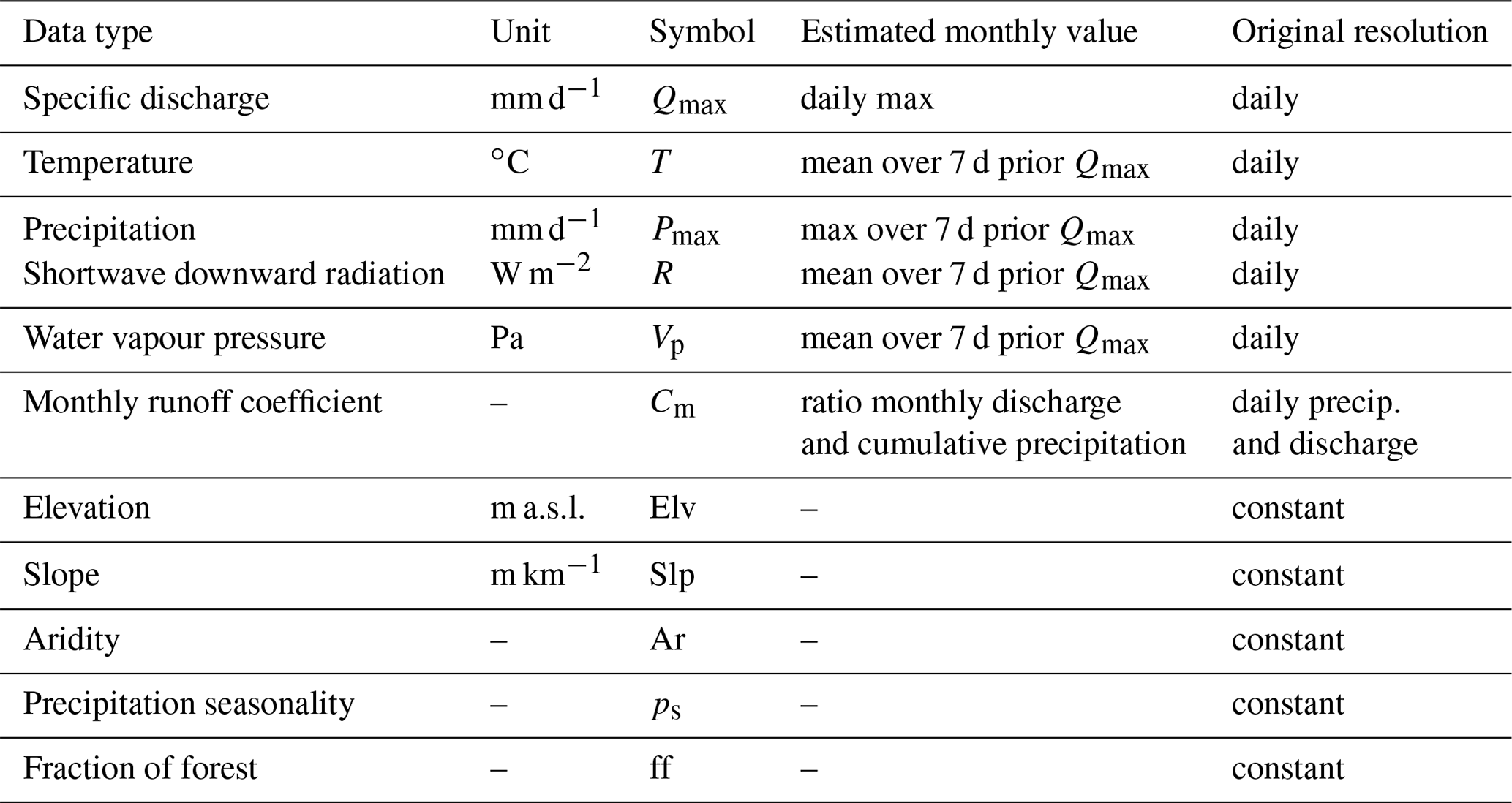
For this study, we make use of the CAMELS data set (Newman et al., 2015; Addor et al., 2017). CAMELS provides homogenised long-term hydro-meteorological data and catchment attributes of catchments across the contiguous United States. To limit potentially adverse effects of spatial heterogeneity, we analyse 240 catchments from the CAMELS data set with areas ≤200 km² (see Table S1 in the Supplement). For each selected catchment, we considered hydro-meteorological data and catchment attributes in Table 1. As the objective of this study is to model maximum daily river discharge in any given month from 1980 to 2013, we further process daily hydro-meteorological data as follows: (1) extract the maximum daily discharge for every given month from daily specific discharge; (2) extract maximum daily precipitation over the previous 7 d from the day of the occurrence of the maximum discharge, and (3) calculate the mean over the previous 7 d from the day of the occurrence of the maximum discharge value of the remaining daily variables. Consequently, we generate a multidimensional data set in which all the variables are related to the occurrence of the maximum daily discharge event in a given month. The selection of these concomitant variables came after a preliminary investigation of the strength of the correlation between maximum discharge and both maximum and cumulative precipitation over different time windows (Fig. S1 in the Supplement). In addition, we investigate whether the maximum precipitation event extracted over the 7 d prior to the maximum daily discharge is also the maximum precipitation event occurring that month. We observe that this is the case almost every month for stations at low to moderate altitude (Fig. S2 in the Supplement), supporting the assumption that in such catchments maximum daily discharge is mainly driven by maximum daily precipitation events in any given month. Such data pre-processing aims to generate a multivariate time series with independent and identically distributed (iid) observations. By selecting maximum daily discharge, we assume that such discharge peaks, and corresponding hydro-meteorological variables, result from different underlying weather events. However, in particular, discharge data do, inevitably and as a result of catchment memory effects, show some degree of autocorrelation (Fig. S3 in the Supplement), which might affect the correlation strength with the remaining variables. We will further discuss this aspect in the Discussion section.

Catchments' attributes from the CAMELS database were used without further processing. The attribute aridity, Ar[–], refers to the ratio of long-term means of potential evapotranspiration calculated using Priestley–Taylor formulation and precipitation, where values higher/lower than 1 indicate water-/energy-limited regions. The attribute precipitation seasonality p_s[–] (Woods, 2009) describes the temporal concentration of intra-annual precipitation occurrence and takes positive/negative values when precipitation peaks occur in summer/winter. For further details on catchment attributes and their derivation, the reader is referred to CAMELS database documentation (Addor et al., 2017).

Table 1 Hydro-meteorological data and catchment attributes used in this study.

Catchments located in the eastern and central-eastern United States (56 %) are characterised by an average size of about 94 km² and average daily specific discharge of 1.3 mm d⁻¹ (Fig. 1a). These catchments are mostly situated at moderate elevations (average altitude 304 m a.s.l.; Fig. 1d) and in energy-limited areas (Ar ∼0.77; Fig. 1b) with little precipitation seasonality (p_s∼0.09; Fig. 1c). In contrast, catchments located in the western and central-western United States (44 %) have an average size of about 61 km² and are on average located at higher elevations, with ∼760 m a.s.l. in the western United States and 2300 m a.s.l. in the central-western region, where precipitation falls mostly over winter (p_s between $\sim -\mathrm{0.9}$ and −0.2; Fig. 1d). While catchments in the western United States are on average located in energy-limited areas (Ar ∼0.6), they are located in water-limited regions in the central-western United States (Ar ∼1.7; Fig. 1b). This difference is reflected in the mean daily discharge, which is 3.1 and 0.64 mm d⁻¹ respectively (Fig. 1a). Catchments in the central-western United States, given their elevation, have the highest ratio of daily precipitation falling as snow in a day with temperatures below zero (∼0.5; Fig. 1e – daily fraction of snow).

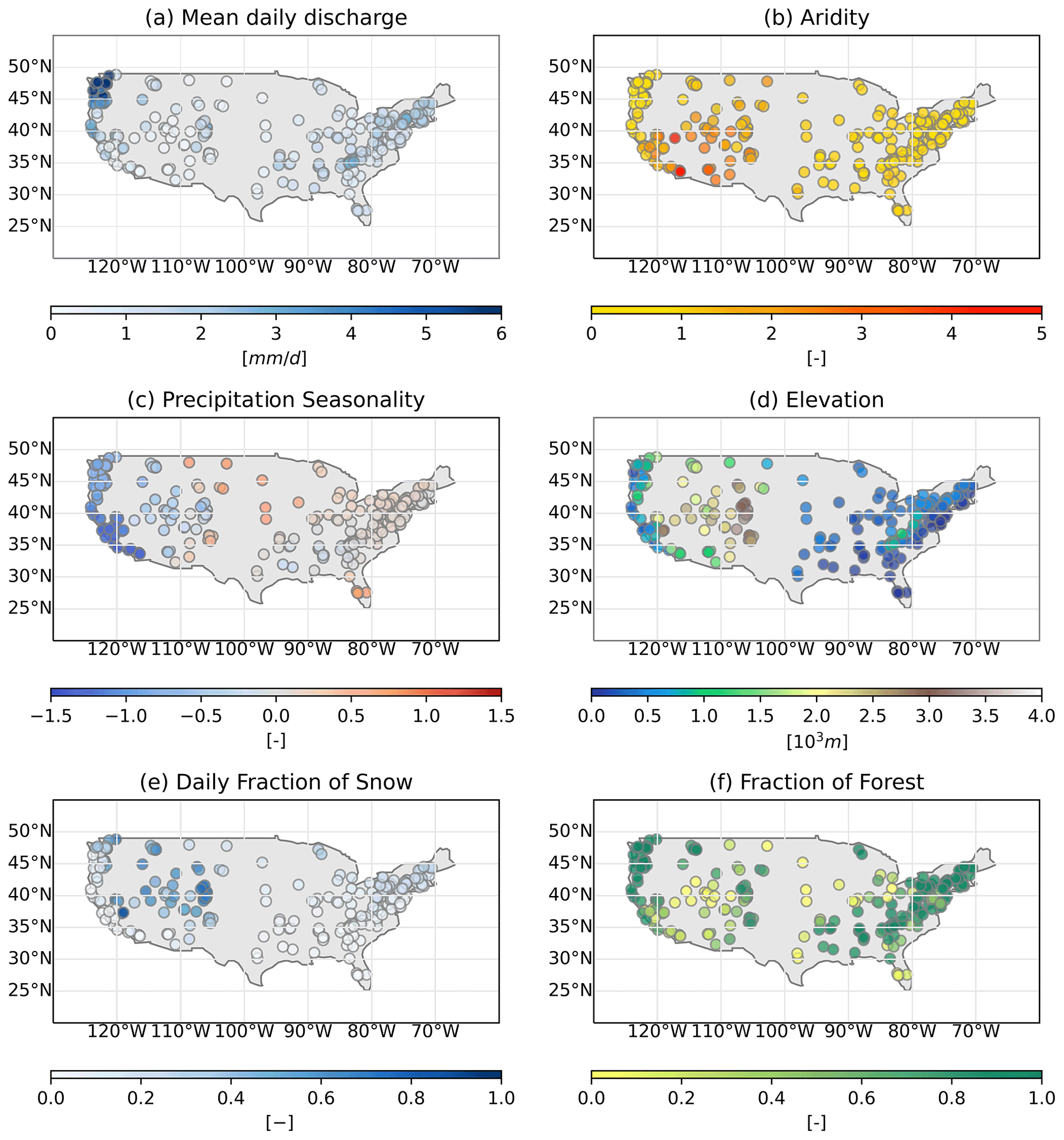
Figure 1 Catchment attributes extracted from the CAMELS database: (a) mean daily discharge (mm d⁻¹); (b) aridity as PET/P; (c) precipitation seasonality, where positive (negative) indicates precipitation peaks in summer (winter); (d) elevation (m a.s.l.); (e) daily fraction of snow indicates the fraction of precipitation falling as snow in the case of temperatures below zero; and (f) fraction of forest.

In the majority of the catchments selected (86 %), the correlation between maximum daily discharge (Q_max) and maximum precipitation over 7 d (P_max) is positive, meaning that discharge is mainly driven by precipitation runoff (Fig. 2a). Catchments with negative correlation are mostly located in water-limited regions (Fig. 2c) and at elevations above 1500 m a.s.l. (Fig. 2b). Furthermore, in such catchments, precipitation occurs mainly in winter, and the fraction of snow is greater than 0.4 (Fig. 2e, f).

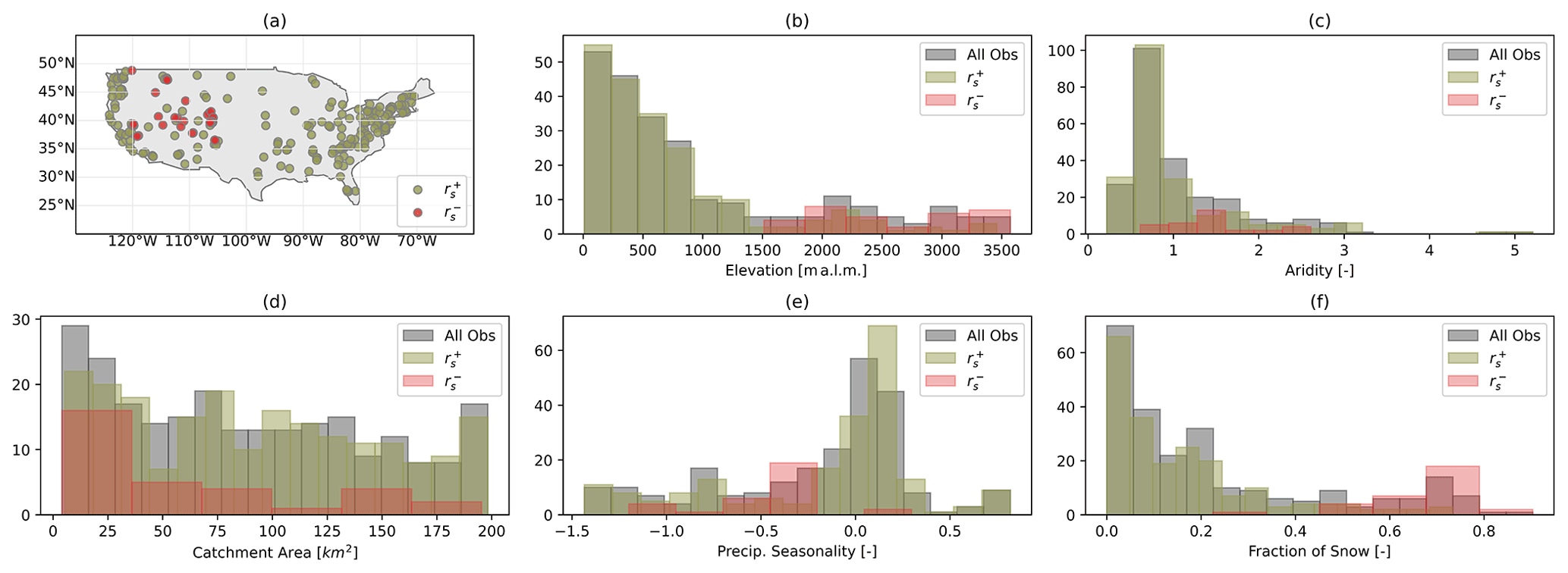
Figure 2 Catchment attributes based on the correlation between maximum daily discharge, Q_max, and maximum precipitation over the previous 7 d, P_max. Panel (a) shows the geographical location of catchments with negative correlation between Q_max and P_max (red dots) and catchments with positive correlation (green dots). Panel (b) shows the distribution of the attribute elevation of catchments with negative (red) and positive (green) correlation against the overall distribution (grey). Panels (c) to (f) show the same comparison as panel (b) but of the following attributes: aridity, area, precipitation seasonality, and fraction of snow respectively.

Hydro-meteorological variables and catchment attributes described so far are used in the following as input to reproduce catchment-scale hydrological dynamics via NPBNs.

3 Probabilistic graphical models: Bayesian networks

Pearl (1985) first formalised the term Bayesian network (BN) as a class of networks represented by influence diagrams or networks to model the probabilistic relationship between variables. Afterwards, BNs became a popular tool for dealing with uncertain domains (Aguilera et al., 2011).

A BN is defined by two components (Aguilera et al., 2011): a qualitative component, being a directed acyclic graph (DAG), where the nodes are the random variables of the model and the arcs connecting two nodes indicate their statistical dependence, and a quantitative component, being the conditional distribution of each variable (child) given its direct preceding variables (parents). Given a network of n nodes (variables) $\mathit{\{}{X}_{\mathrm{1}},\mathrm{\dots },X_n\mathit{\}}$ and a set of parent nodes S_i for node i, the joint density (mass in the discrete case) is defined as

$$\begin{array}{}\text{(1)}& f(x_{\mathrm{1}},\mathrm{\dots },x_n)=\prod _{i=\mathrm{1}}^n{f}_{x_i|S_i}\left(x_i\right|S_i).\end{array}$$

The (conditional) independence relationships embedded in the probabilistic model can be easily visualised in the graphical representation of the network (Pearl, 1985). Moreover, the absence of an arc guaranties the conditional independence between two “source” variables (Hanea et al., 2015), while the direction of the arc indicates the “flow of information” (Vogel et al., 2014). Strictly speaking, probabilistic dependence does not have a “direction”. However, when it can be easily related to causality, it is convenient to think of a flow of information.

BNs differ on how nodes and arcs are quantified, and the inference process depends on this quantification. Discrete BNs specify the source nodes, i.e. nodes without parents, as discrete random variables and conditional probability tables for child nodes (Hanea et al., 2006). Hybrid BNs (HBNs) involve both discrete and continuous variables. HBNs specify marginal distributions for nodes without parents and conditional distributions for child nodes. HBNs can be fully parametric, in which marginals and joint probabilities are from parametric families, or fully discrete, in which continuous variables are discretised (Hanea et al., 2015). Discretisation of continuous variables, however, has the drawback of requiring a very large number of partitions to guarantee a good approximation of the variables.

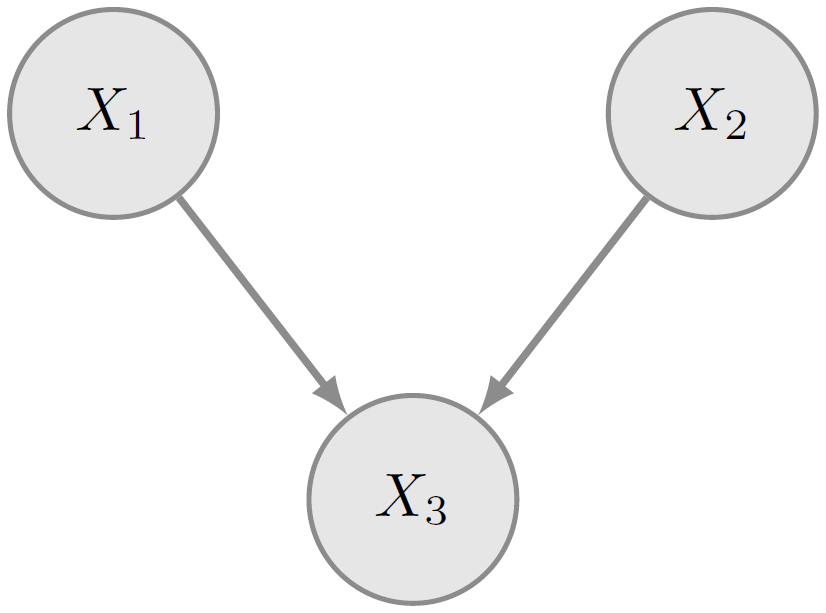
Figure 3 is an illustrative example of the qualitative component of a BN for the variables $\mathit{\{}{X}_{\mathrm{1}},X_{\mathrm{2}},X_{\mathrm{3}}\mathit{\}}$. The quantitative component is given by $f_{X_{\mathrm{1}}}\left(x_{\mathrm{1}}\right)$, $f_{X_{\mathrm{2}}}\left(x_{\mathrm{2}}\right)$, and $f_{X_{\mathrm{3}}|S_{\mathrm{3}}}\left(x_{\mathrm{3}}\right|S_{\mathrm{3}})$, where $S_{\mathrm{3}}=\mathit{\{}{X}_{\mathrm{1}},X_{\mathrm{2}}\mathit{\}}$ is a set containing the parents of node X₃. The joint probability resulting from the above information is $f(x_{\mathrm{1}},x_{\mathrm{2}},x_{\mathrm{3}})=f_{X_{\mathrm{1}}}\left(x_{\mathrm{1}}\right)\cdot f_{X_{\mathrm{2}}}\left(x_{\mathrm{2}}\right)\cdot f_{X_{\mathrm{3}}|S_{\mathrm{3}}}\left(x_{\mathrm{3}}\right|S_{\mathrm{3}})$. From Fig. 3, it is possible to determine the dependence relationships between the nodes. The absence of the arc connecting X₁ and X₂ implies their independence (X₁⟂X₂). However, X₁ and X₂ are conditional dependent on when information on X₃ becomes available; i.e. X₁ and X₂ are dependent given X₃ ($X_{\mathrm{1}}\cancel{⟂}{X}_{\mathrm{2}}|X_{\mathrm{3}}$).

Figure 3 Illustrative Bayesian network with three nodes.

3.1 Non-parametric Bayesian networks

Kurowicka and Cooke (2005) introduced a vine-copula-based approach for HBNs called non-parametric Bayesian networks (NPBNs). NPBNs specify the nodes as arbitrary invertible distribution functions and the arcs as (conditional) rank correlations realised by a chosen one-parameter bivariate copula (Kurowicka and Cooke, 2005). This construction has two main implications: the parent–child dependence is realised by bivariate pieces of dependence, and the information required to quantify the network reduces to a number of marginal distributions equal to the number of nodes and a number of (conditional) dependence parameters (parameterised by Spearman's rank correlation) equal to the number of arcs in the network (Hanea et al., 2015).

Hanea et al. (2015) demonstrated that the vine-copula-based approach determines a unique joint distribution of the n nodes given: (1) a DAG with n nodes specifying the conditional independence relationships; (2) n variables $\mathit{\{}{X}_{\mathrm{1}},\mathrm{\dots },X_n\mathit{\}}$ assigned to the nodes and described by invertible marginal distributions $\mathit{\{}{F}_{\mathrm{1}},\mathrm{\dots },F_n\mathit{\}}$; (3) arcs $i_{\mathrm{p}-k}\to i$ for the node i and its ordered set of p parent nodes $S_i=\mathit{\{}{i}_{\mathrm{1}},\mathrm{\dots },i_{\mathrm{p}}\mathit{\}}$ specified by the (conditional) rank correlation in Eq. (2); and (4) a copula realising the (conditional) correlations in (3), for which correlation 0 denotes independence. It is worth noting that the parent set S_i for node i does not have a unique order.

$$\begin{array}{}\text{(2)}& \left\{\begin{array}{ll}{r}_{i,i_{\mathrm{p}-k}},& k=\mathrm{0}\\ r_{i,i_{\mathrm{p}-k}|i_{\mathrm{p}},\mathrm{\dots },i_{\mathrm{p}-k+\mathrm{1}}},& \mathrm{1}\le k\le p-\mathrm{1}\end{array}\right.\end{array}$$

Considering the DAG in Fig. 1, the joint probability of the associated NPBN is uniquely quantified given invertible marginal distributions $\mathit{\{}{F}_{\mathrm{1}},F_{\mathrm{2}},F_{\mathrm{3}}\mathit{\}}$ and the (conditional) rank correlation for the two arcs r_1, 3 and $r_{\mathrm{2},\mathrm{3}|\mathrm{1}}$, or r_2, 3 and $r_{\mathrm{1},\mathrm{3}|\mathrm{2}}$ depending on the parent ordering for node 3.
The choice of the copula to quantify the arcs is arbitrary. However, only the joint normal copula allows for rapid calculation and inference for complex problems (Hanea et al., 2015). For this reason, in this study, we adopt the protocol presented in Hanea et al. (2006) based on the Gaussian-copula assumption. This protocol computes the joint distribution function of n variables $\mathit{\{}{X}_{\mathrm{1}},\mathrm{\dots },X_n\mathit{\}}$ with invertible marginal distributions $\mathit{\{}{F}_{\mathrm{1}},\mathrm{\dots },F_n\mathit{\}}$ by the following:

• The set of variables X is transformed in standard normal variables Y via the transformation $Y_i={\mathrm{\Phi }}^{-\mathrm{1}}\left(F_i\right(X_i\left)\right)$ for each node i, where Φ is the univariate standard normal distribution. The transformation is strictly increasing, so after the transformation the (conditional) rank correlation is unchanged.

• To each arc of the network, the quantity ${\mathit{\rho }}_{i,j|D}=\mathrm{2}\sin (\mathit{\pi }\cdot r_{j,i|D}/\mathrm{6})$ is assigned, where (i,j) and D are the conditioned and the conditioning set respectively, and $r_{j,i|D}$ and ${\mathit{\rho }}_{i,j|D}$ are the conditional rank correlation and the partial product moment of the normal variables respectively. A unique joint normal distribution, and so a unique correlation matrix, satisfying the partial correlation specification is determined.

• The correlation matrix R is computed recursively based on the partial correlations.

The joint distribution of the initial variables X and their specified dependence is then realised by sampling a sample $\stackrel{\mathrm{̃}}{Y}$ from the joint normal distribution with correlation matrix R and transforming it back to its original units via ${\stackrel{\mathrm{̃}}{X}}_i=F_i^{-\mathrm{1}}\left(\mathrm{\Phi }\right({\stackrel{\mathrm{̃}}{Y}}_i\left)\right)$ for every node i.

NPBNs based on the normal copula assumption are implemented in the open-source MATLAB toolbox BANSHEE (Paprotny et al., 2020), which is used in this study to carry out the analyses.

4 NPBNs as a model for river discharge generation

The aim of this study is to investigate the suitability of NPBNs to reproduce catchment-scale hydrological dynamics. The rationale adopted to identify suitable DAG consists of representing a catchment as a system in which discharge is generated by the interaction between the input of the system, for example, precipitation, the state of the system, for example, soil moisture, and the output of the system, for example, river discharge (Fig. 4a). This schematisation allows us to define, via the associated NPBN, the joint probability distribution function of the variables (nodes) representing the input, state, and output of the system catchment and subsequently infer the variable of interest, i.e. river discharge, via conditioning on the remaining variables. This schematisation, hereafter graph type I, can easily be extended to include additional variables, such as physical attributes (e.g. elevation) of the system catchment, resulting in the schematisation in Fig. 4b, hereafter graph type II. Graph type I determines the joint probability distribution of input (I), output (O), and state (S) of a catchment considered as a single element; i.e. the nodes are defined by the observations taken at one single catchment. Such joint distributions can be used to infer information on that single catchment. On the other hand, graph II defines the joint probability distribution of input (I), output (O), state (S), and attribute (A) of the catchments, and the nodes are defined by pooled observations derived by merging observations at multiple locations. This way of defining the nodes implies that also the attribute nodes, which are constant value in time for a given catchment, become random variables, and so they can be modelled as additional nodes in the network. From the joint distribution defined by graph type II, we can derive the joint probability distribution of the input, output, and state variables of one single catchment; i.e. graph type I, via conditioning on the attributes of that catchment, $F_{g-I}(I,O,S)=F_{g-II}(I,O,S|A_{g-I})$. $F_{g-I}(I,O,S)$, derived from conditioning $F_{g-II}(I,O,S,A)$, benefits from information provided by similar catchments. Graph type II can then be implemented for ungauged catchments by exploiting information from gauged catchments with similar attributes.

In graph type I, the following continuous hydro-meteorological variables will be considered here: P_max, T, R, V_p, (input), Q_max (output), and C_m (proxy for system state component). In graph type II, the following nodes are added: Elv, Slp, Ar, p_s, and ff (system attributes, Table 1). It is worth mentioning that in a preliminary analysis (not shown here), we tested the use of ESA CCI (https://esa-soilmoisture-cci.org/, last access: 27 November 2018) remote sensing soil moisture data since measurements are available from 1978, similarly to the CAMELS data set. However, the presence of missing values significantly affected the length of the multivariate data set of hydro-meteorological variables considered for training and testing the networks of interest. Moreover, the coarse spatial resolution and the time lag between the response of river discharge and soil moisture to external input, such as precipitation, led us to rather use the monthly runoff coefficient here as a proxy for system state. A more in-depth discussion is presented in Sect. 6 – Discussion and challenges.

Network selection, i.e. moving from a graph to a DAG by selecting arcs connecting a given set of nodes to model dependence, is challenging due to the high number of possible configurations describing a given set of variables. In this study, we selected two DAGs a priori: a DAG in which the variables are parent nodes, with one child being the variable Q_max, and a DAG in which all the variables are connected via arcs, resulting in a saturated network. We will refer to them as the unsaturated network (UN) and saturated network (SN) respectively. UN can be considered as a multilinear regression function in which the discharge is the dependent variable, and the remaining variables are the independent (explanatory) variables, with coefficients defined by the rank correlation between the variables and discharge. Such explanatory variables are assumed to be independent of each other. However, in such a network, discharge is inferred as a function of all the other variables, while the other variables, for example, P_max, T, R, V_p, and C_m, only depend on the discharge. This implies that this unsaturated network is suitable only if the variable to be inferred is determined a priori, as in this case discharge, since our interest is in reproducing river discharge. SN, on the contrary, accounts for the interdependence of all the variables and does not have a pre-defined variable of interest which can influence the design of the network structure, as in UN. However, network selection, i.e. number and direction of the arcs and parent nodes ordering, is to some extent arbitrary. In addition, the strength of the arcs, determined by the dependence between nodes, can be based entirely on observations, as in this study, but can also be elicited from experts (Morales et al., 2008; Hanea et al., 2010). Hence, network definition and selection will be further discussed in Sect. 6 – Discussion and challenges.

In this study, we investigate two networks, one unsaturated (hereafter UN-1), as shown in Fig. 4c, and one saturated (hereafter SN-1), as shown in Fig. 4d, to generate river discharge considering each catchment as a single element.

To further explore the applicability of NPBNs in hydrological studies, we investigate the potential of a single saturated network (hereafter SN-C, Fig. 4e) to reproduce maximum daily river discharge over many catchments and eventually also in ungauged basins. Such a network builds upon the SN-1 network and, in addition, includes attribute nodes. We implement the SN-C network on a subsample of the 240 catchments with a positive correlation between P_max and Q_max and Nash–Sutcliffe efficiencies (NSEs) ≥ 0.5, calculated using the SN-1 network. In doing so, we group catchments with a similar property and performance at the catchment level a priori. From the SN-C network, we only infer statistical characteristics of river discharge rather than specific events, as we do from UN-1 an SN-1.

The joint distribution function associated with each network (UN-1, SN-1, and SN-C) is derived following the protocol presented in Hanea et al. (2006) and discussed in the previous section. We assume a normal copula for quantifying (conditional) rank correlations and empirical cumulative distribution functions for describing the marginal distributions of the different nodes.

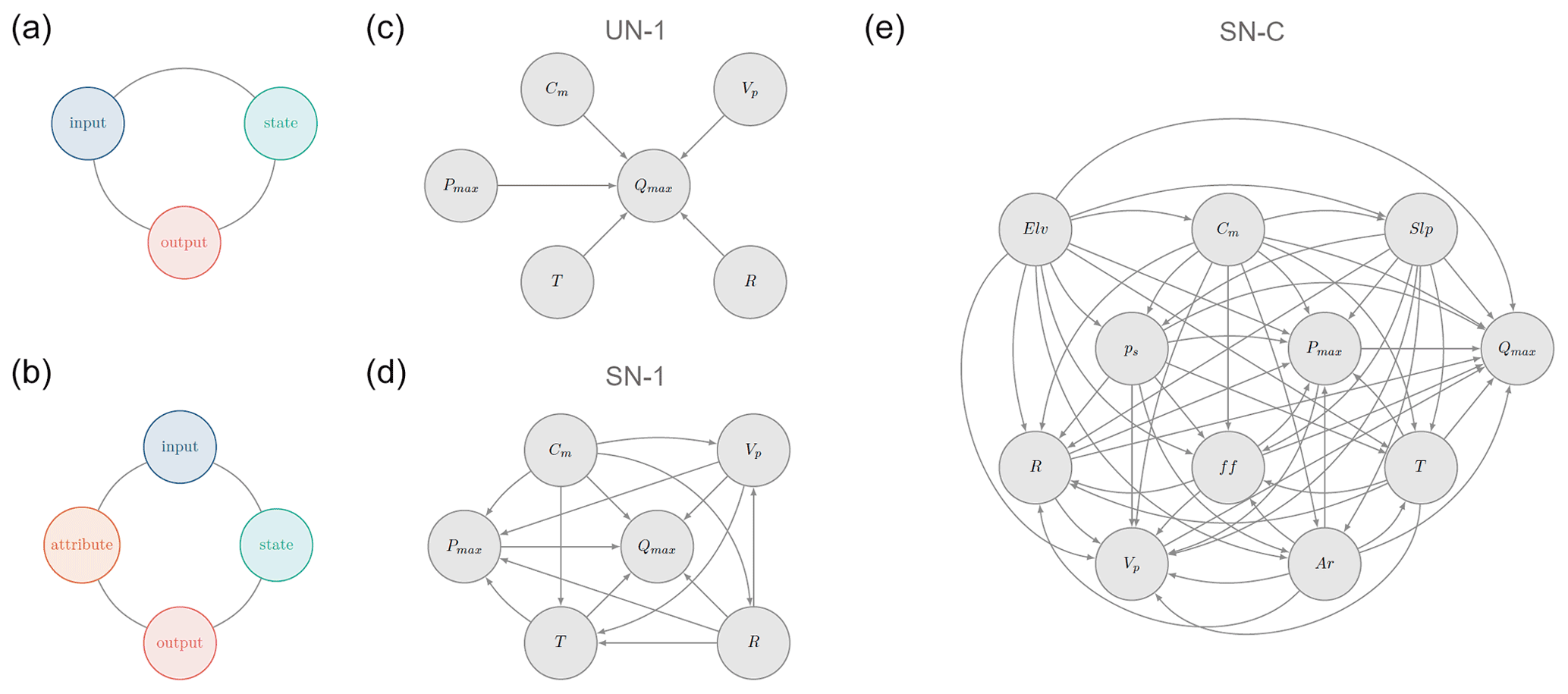
Figure 4 Graphs and qualitative networks (DAGs) used in this study. Panels (a) graph type I and (b) graph type II show the rationale underlying the selection of the variables in the networks. Panels (c) and (d) represent the networks for analysing catchments as single elements, UN-1 and SN-1 respectively. Panel (e) shows the network for analysing a group of catchments from contrasting climates, SN-C.

4.1 NPBN testing

To assess the potential of NPBNs as probabilistic models for catchment dynamics, we first test the networks (UN-1, SN-1, and SN-C) as descriptive models. Subsequently, we evaluate the networks as predictive models. In this study, the term testing process refers to analyses performed on the descriptive models, while the term evaluation process refers to analyses performed on predictive models. In the evaluation process, elsewhere also referred to as validation process, the data set used to determine the networks, i.e. quantification of the dependence between nodes, differs from the data set used to evaluate the performance of the network in estimating discharge. In the testing process, elsewhere also referred to as verification process (Hanea et al., 2015), the entire set of observations available is used to first determine the networks and then to test it via diagnostic metrics, such as the NSE and Kolmogorov–Smirnov (KS) test here. This approach implies that the minimum requirement for a network is to reproduce the observations used for quantifying the model itself. At the same time, it can happen that the limited number of available observations does not allow for the definition of a representative training set and a test set (Hanea et al., 2015), preventing the possibility of evaluating the predictive capabilities of the model. In the evaluation process, we perform a k-fold cross-validation by randomly selecting 10 years, between 1980 and 2013, as a test set, while the remaining years are used as a training set.

In both the testing and evaluation process, we first test the assumption of the joint normal copula for modelling the bivariate dependence via the Cramér–von Mises test. Then, we use the d-calibration score to test the assumption that the network selected, UN-1, SN-1, or SN-C, can model the overall multivariate dependence structure. Afterwards, we test and evaluate the performances of the networks as descriptive and predictive models, respectively, in inferring discharge data via the two-sample Kolmogorov–Smirnov (KS) test and the Nash–Sutcliffe efficiency (NSE) coefficient.

The Cramér–von Mises (CvM) statistic S provides an indication of the distance between the empirical copula C_n and the theoretical copula C_θ, for example, Gaussian copula (Genest and Favre, 2007):

$$\begin{array}{}\text{(3)}& S=n\sum _{i=\mathrm{1}}^n\mathit{\left\{}{C}_n\right({\displaystyle \frac{R_i^{\mathrm{1}}}{n+\mathrm{1}}},{\displaystyle \frac{R_i^{\mathrm{2}}}{n+\mathrm{1}}})-C_{\mathit{\theta }}({\displaystyle \frac{R_i^{\mathrm{1}}}{n+\mathrm{1}}},{\displaystyle \frac{R_i^{\mathrm{2}}}{n+\mathrm{1}}}){\mathit{\}}}^{\mathrm{2}},\end{array}$$

where $R_i^{\mathrm{1}}$ and $R_i^{\mathrm{2}}$ are the ith ranks of the n observations. The CvM test provides a measure of goodness of fit of a theoretical copula. S=0 means a perfect fit. We test the normal copula assumption in modelling dependence via bivariate correlation by performing the CvM test on the pairs of variables resulting from the combination of the network nodes (variables). We compare the empirical copula of each pair with four different parametric copulas, widely used in hydrological studies, namely Gaussian (or normal), Frank, Gumbel, and Clayton. The characteristics of the Gaussian and the Frank copula are similar, in the sense that they are both suitable models for variables which do not have a strong association between each other when both take low/high values. On the other hand, Gumbel and Clayton copulas are suited to model variables with a strong dependence at the upper and lower tail, respectively.

The d-calibration (d_c) metric (Morales-Nápoles et al., 2014b) is a goodness-of-fit measure of the joint probability distribution function defined via NPBN against the empirical distribution.

$$\begin{array}{}\text{(4)}& d_{\mathrm{c}}=\mathrm{1}-d_{\mathrm{h}},\end{array}$$

where d_h is the Heillinger distance between the empirical correlation matrix of the variables (nodes of the network) and the NPBN correlation matrix. d_c takes values between 0 and 1, with a high score implying that the two correlation matrices are similar.

The two-sample Kolmogorov–Smirnov (KS) is a non-parametric hypothesis testing technique assessing whether two samples, Y and $\stackrel{\mathrm{̃}}{Y}$, belong to the same population (Massey, 1951). The KS test statistic D^* is defined as

$$\begin{array}{}\text{(5)}& D^{*}=\underset{y}{max}\left(\right|F_Y\left(y\right)-F_{\stackrel{\mathrm{̃}}{Y}}\left(y\right)\left|\right).\end{array}$$

The null hypothesis H₀ is F_Y = $F_{\stackrel{\mathrm{̃}}{Y}}$ against alternatives. In this study, we consider a level of significance α=0.05.

The Nash–Sutcliffe efficiency coefficient (NSE) (Nash and Sutcliffe, 1970) measures the predictive capabilities of the NPBN.

$$\begin{array}{}\text{(6)}& \mathrm{NSE}=\mathrm{1}-{\displaystyle \frac{{\sum }_{i=\mathrm{1}}^N(y_{\mathrm{sim}}^i-y_{\mathrm{obs}}^i)}{{\sum }_{i=\mathrm{1}}^N(y_{\mathrm{obs}}^i-{\stackrel{\mathrm{‾}}{y}}_{\mathrm{obs}})}},\end{array}$$

where y_sim is the simulated specific discharge, y_obs is the observed specific discharge, ${\stackrel{\mathrm{‾}}{y}}_{\mathrm{obs}}$ is the observation mean, and N is the total number of observations. Values of NSE lower than 0 indicate that the observation mean (${\stackrel{\mathrm{‾}}{y}}_{\mathrm{obs}}$) is a better predictor than the model adopted. Values close to 1 suggest very good model performances.

NPBN treats hydro-meteorological data and catchment attributes as random variables. This implies that during the inference process, the NPBN returns, at each time step, a conditional distribution function of the target variable, i.e. the distribution of maximum daily river discharge conditioned on the remaining hydro-meteorological data and attributes. From this conditional distribution of river discharge, 1000 possible discharge realisations are sampled, and the 50th percentile is taken as the estimated discharge value for that particular combination of hydro-meteorological data and attributes. Similarly, the confidence interval (CI) of the estimated discharge value is determined as the 5th and the 95th percentile of the 1000 realisations of the conditional distribution.

5 Results

In this section, we first show the potential of NPBNs in estimating maximum daily river discharge when a catchment is modelled as single elements. Afterwards, we present the capability of NPBNs to model catchments in a cluster to eventually infer river discharge of an ungauged basin given its attributes.

5.1 Catchment as single elements

We first analyse the performances of the UN-1 and SN-1 networks as descriptive models. In Fig. 5a, the results of the CvM test show that the best copula model among the four tested is the Frank copula for ∼55 % of the pairs, the Gaussian copula for ∼10 %, and the Gumbel and Clayton for ∼20 % of the pairs respectively. This suggests that about 65 % of the pairs, i.e. pairs best modelled with either Frank or Gaussian copula, show a dependence without a strong association between low and high values. Hence, this result supports the normal copula assumption of NPBNs, since the Gaussian copula is a suitable model for such type of dependence. In Fig. 5b, boxplots summarising the results in terms of d-calibration score indicate that, on average, the SN-1 network, with a median of ∼0.8, better captures the overall dependence between variables. Indeed, the d-calibration score compares the empirical correlation matrix of the variables with the correlation matrix resulting from the DAG. A low d-calibration score for the UN-1 network (median of ∼0.25) can be linked to the strong assumption of independence between pairs of variables in which one variable in the pair is not discharge. A further insight about the suitability of the UN-1 and SN-1 networks is via NSE, which describes how a network is able to reproduce discharge events given information about P_max, T, R, V_p, and C_m. For catchments in which the correlation between Q_max and P_max is negative, i.e. catchments in water-limited regions and at high elevations, the SN-1 network returns a higher value of NSE compared to the UN-1 network (red dots above the identity line; Fig. 5c). This result provides evidence that, in catchments where the discharge generation process is not predominantly precipitation driven, it is important to account for the interaction between other hydro-meteorological variables and catchment current state. Finally, based on the expected Q_max simulated with the network, for each catchment, we estimated the 0.5, 0.05, and 0.95th quantile, and we compare them with the same quantiles from observations. While the observed and simulated mid-quantiles in both the UN-1 and SN-1 networks, respectively, broadly correspond (Fig. 5d), Fig. 5e shows that in the SN-1 network, lower quantiles are overestimated (dark grey histogram with most mass on values >1), while upper quantiles are underestimated (dark grey histogram with most mass on values <1; Fig. 5f). Conversely, the UN-1 network shows greater variability in simulating discharge since a clear pattern of over- or underestimation is not visible, especially for the 0.95th quantiles (Fig. 5f). These results likely reflect the property of the Gaussian copula of no tail dependence.

The preliminary analysis on the descriptive capabilities of the UN-1 and SN-1 networks suggests that the SN-1 network is better suited for describing the dynamics of river discharge compared to UN-1. However, when we look more in depth into SN-1 network performances, we can observe that only 66 % of the catchments have a NSE higher than 0.5 (Fig. 6a), which in the literature is considered as an acceptable performing model (Moriasi et al., 2007; Newman et al., 2015). Such catchments receive precipitation mainly in winter (mean $p_{\mathrm{s}}\sim -\mathrm{0.19}$), are located in energy-limited regions (mean Ar ∼0.78), and are mostly green areas (mean fraction of forest ∼0.91). At the same time, in 85 % of the catchments, the H₀ of the KS test cannot be rejected (average p value = 0.49), suggesting that the sample of maximum daily river discharge simulated from the network derives from the same distribution as the sample observed. This result implies that the network captures the average behaviour of the catchment well in the long term (tested via KS test), while it has limitations when inferring single events (tested via NSE).

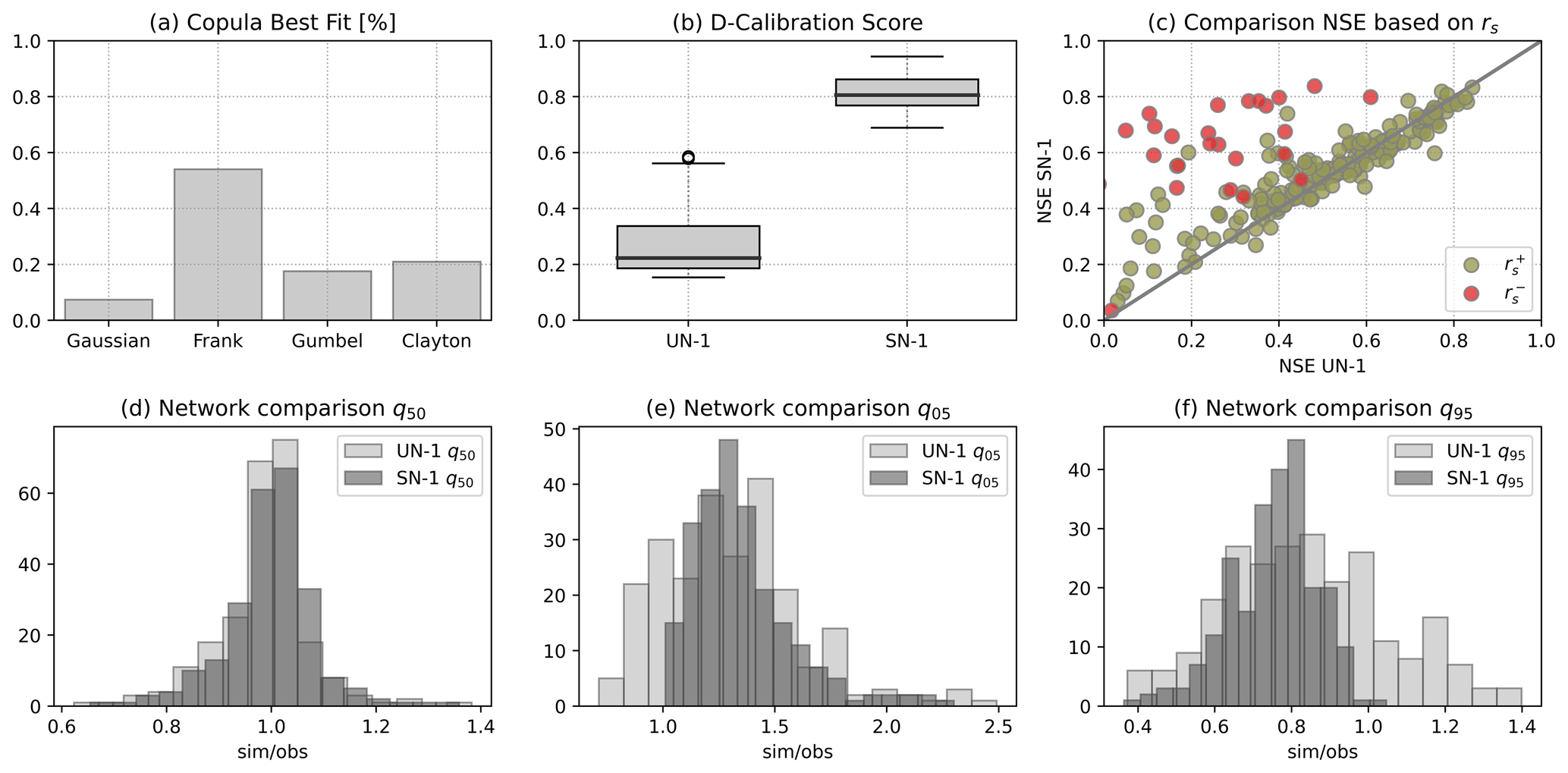
Figure 5 Results of the testing process when the UN-1 and SN-1 networks are used as descriptive models of the 240 catchments considered as single elements. Panel (a) shows the percentage of pairs with the copula on the x axis as best fit. Panel (b) shows the variability of the d-calibration score across catchments. Panel (c) shows the comparison between UN-1 and SN-1 in terms of NSE as a function of the sign of the correlation (r_s) between Q_max and P_max. Red dots indicate negative correlation ($r_{\mathrm{s}}^{-}$), while green dots ($r_{\mathrm{s}}^{+}$) indicate positive correlation. The identity line (grey) is used as an indicator to visually compare the results from UN-1 and SN-1 networks. Dots on the line indicate matching results between the two networks, while dots above/below the line indicate higher values of NSE associated with the NS-1/UN-1 network. Panels (d) to (f) show the histograms of the ratio between simulated and observed discharge quantiles, i.e. 0.5, 0.05, and 0.95th quantiles, for the UN-1 (light grey) and SN-1 (dark grey) network. Panel (d) shows that the UN-1 and SN-1 networks simulate the 0.5th quantile similarly, while panel (e) and (f) show that the SN-1 network generally over- and underestimates the 0.05 and the 0.95th quantile respectively. Panel (e) and (f) show also that the UN-1 network does not have a clear tendency to over- or underestimate the quantiles.

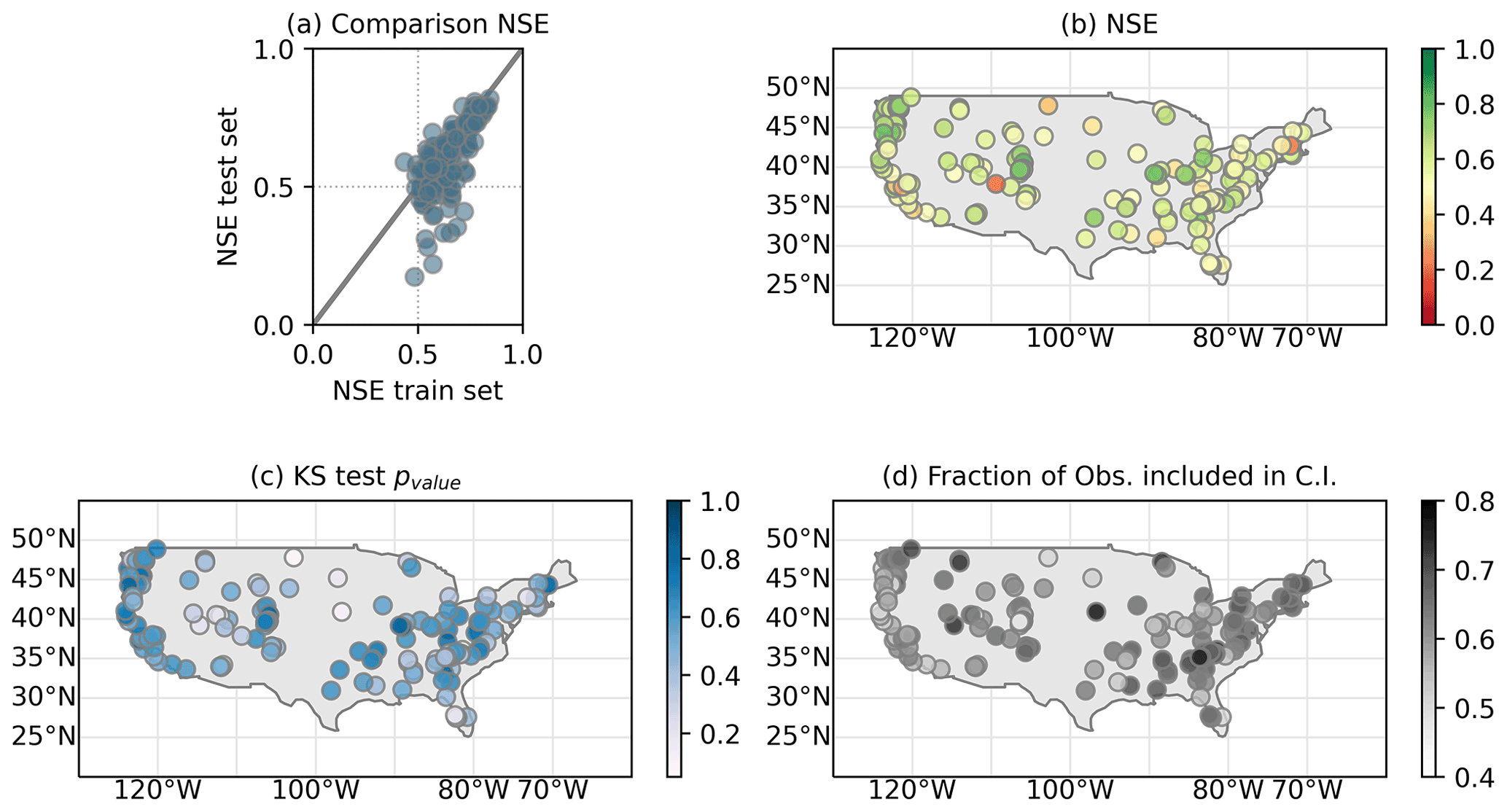
Figure 6 Performances of the SN-1 network in terms of NSE for the 159 catchments with NSE ≥0.5 in the testing process. Panel (a) compares the performances of the training and test set. Panel (b) shows the value of NSE per catchment. Panel (c) shows the p value resulted from the KS test per catchment. Panel (d) shows the overall fraction of observations falling inside the estimated discharge uncertainty bounds per catchment.

To further investigate the ability of NPBNs to estimate maximum daily river discharge, we evaluate the performances of the SN-1 network as a predictive model. We limit the investigation to the SN-1 network since the above results suggest that it is a descriptive model for a larger number of catchments with contrasting characteristics compared to the UN-1 network. The k-fold cross-validation test is applied to catchments with a NSE greater than 0.5 in the testing process described above, here 159 catchments. We perform five simulation runs, and, in every run, 10 years were randomly selected as the test set. We consider the performances in terms of NSE calculated as mean value of the five runs. Results indicate that 25 % of the catchments have a higher NSE in the test set than the training set (Fig. 6a). In general, one would expect a better performance in the test set compared to the training set, since the metric for evaluating model performances uses the same data set for quantifying and testing the model. Hence, the fact that the training set performs better than the test set could depend on the random selection of the years for evaluating the network. This random procedure might have split the original data set into two data sets with different characteristics. This could be due to the relatively small number of years of observations which are subsequently divided into even smaller data sets. In contrast, around 55 % of the catchments analysed (about 40 % of the total catchments) have a NSE in the test set ≥0.5 (Fig. 6b) and, at the same time, a NSE in the test set equal to or lower than the training set (Fig. 6a), meaning that the SN-1 network in these catchments provides reliable estimates of river discharge events and long-term characteristics. In a recent study, Ren et al. (2020) investigated the performances of regression models based on a variety of filter-based feature selection methods to estimate average monthly river discharge in three catchments from the CAMELS data set. The results obtained in terms of NSE ranged from ∼0.6 to ∼0.8, values similar to the average (mean) performance of the SN-1 network (NSE ∼0.596), investigated here for maximum daily river discharge. Kratzert et al. (2019) used CAMELS data set to evaluate the performances of hydrological models. They investigated the performances of the long short-term memory (LSTM) network to estimate daily river discharge in 530 catchments and included also, among other models, the performances of the Sacramento Soil Moisture Accounting (SAC-SMA) conceptual model. For the sake of discussion, we look at the performances of the LSTM network without catchments' attributes and SAC-SMA from Kratzert et al. (2019) for a subset of catchments also analysed in this study. The results of Kratzert et al. (2019) are available at https://github.com/kratzert/lstm_for_pub (last access: 6 October 2021). The LSTM network without catchment attributes and the SAC-SMA conceptual model for daily river discharge have an average (mean) performance of NSE ∼0.603 and ∼0.598 respectively. The SN-1 network, investigated here, for maximum daily river discharge, has an average (mean) performance of NSE ∼0.596. In general, NSEs obtained for simulations on a daily temporal scale tend to be lower than the ones on a monthly temporal scale due to the higher number of observations over a common fixed period of time (Moriasi et al., 2007). However, other studies suggest that for both daily and monthly model simulations, a satisfactory performance is given when 0.37 < NSE < 0.75 (Van Liew et al., 2007). To further evaluate the performance of NPBNs for maximum river discharge, we perform the KS test. In about 95 % of the catchment, the KS test H₀ cannot be rejected (Fig. 6c). Such a result is in agreement with the one found in the testing process of the descriptive model, that the SN-1 network shows limitations when inferring single events (tested via NSE) but is fairly good when inferring long-term behaviour (tested via KS).

NPBNs provide a quantification of the uncertainty around the estimated river discharge values. We then quantify the uncertainty of the estimated maximum river discharge. On average and across all catchments, observed discharge in the test set falls within the simulated confidence interval (5th and 95th percentile) about 63 % of the time, ranging between a minimum of 45 % and a maximum of 78 % (Fig. 6d).

Figure 7 Comparison between maximum daily river discharge simulations from run 1 and observations of three different catchments. The grey shaded areas indicate years belonging to the test set. The shaded red areas represent the simulation confidence interval evaluated as the 5th and the 95th percentile.

To further evaluate the results of the SN-1 network in estimating maximum daily river discharge, the hydrograph of three stations, i.e. no. 6746095 (Colorado), no. 11481200 (California), and no. 14306340 (Oregon), with contrasting characteristics are shown in Fig. 7.

The catchment in Colorado is located in a water-limited area (Ar ∼1.1) above 3000 m a.s.l., it has a negative correlation between Q_max and P_max, and precipitation falls mainly in winter (negative value of p_s). The results of the evaluation process show that the SN-1 network can reproduce the statistical characteristics of the maximum river discharge observed (KS-H₀ non-rejected, p value = 0.82) as well as the seasonal variability (Fig. 7d). Moreover, the scatter plot in Fig. 7a shows simulations in agreement with observations (mean absolute percentage error (MAPE) ∼0.47). The mean value of NSE across the five runs is 0.82, and 56 % of the observations fall within the simulation confidence interval (Fig. 7d). The catchment in California is located in an energy-limited region (Ar ∼0.54) at ∼300 m. a.s.l. Here, there is a positive correlation between Q_max and P_max, and precipitation falls mainly in the winter season (negative p_s). The SN-1 network is able to simulate the statistical characteristics of the observed discharge (KS-H₀ non-rejected, p value = 0.72). Moreover, the simulations follow the seasonal variability of the observations (Fig. 7e), even though it is less pronounced than in Colorado, and ∼50 % of the observations fall within the model CI. The mean value of NSE across the five runs is 0.68, and the MAPE is ∼0.83. This result reflects the fact that few simulations in the test set (Fig. 7b) deviate significantly from observations. Finally, the catchment in Oregon is located in an energy-limited region (Ar ∼0.38) at ∼400 m. a.s.l., and it has a positive correlation between Q_max and P_max. Precipitation falls mainly in the winter season (negative p_s). The SN-1 network is able to reproduce the statistical characteristics of maximum river discharge (KS-H₀ non-rejected, p value = 0.86), and the discharge seasonal variability is captured by the model (Fig. 7f). The NSE across the five runs is 0.79, and MAPE is ∼0.60. In the hydrograph in Fig. 7f, it can be observed that in 2001, the seasonal variability typical of the other years is less pronounced. Also, the CI (shaded red area) is larger compared to the rest. This is likely a consequence of the fact that 3 consecutive years (1999, 2000, and 2001; Fig. 7f) were randomly selected for model evaluation, including the year 2001.

These results show the potential of the SN-1 network to model the river discharge generation process in catchments with contrasting climate exploiting information from the interaction between the different inputs of the system catchment, i.e. R, V_p, T, P, and C_m, even when precipitation is not the main discharge driver, for example, in Colorado.

5.2 Catchments in a cluster

We implement the SN-C network on a subsample of 133 catchments with a positive correlation between P_max and Q_max and NSE calculated based on the SN-1 network greater than 0.5 in the previous analysis considering catchments as single elements.

We first test the performance of the SN-C network as a descriptive model. Similar to the results obtained previously, Frank and Gumbel copulas are the best theoretical copulas for about 50 % of the pairs, supporting the choice of the NPBN. The d-calibration score is about 0.84, meaning that the network captures the interdependence between variables obtained via the empirical correlation matrix well. In contrast, the KS test indicates that in only 20 % of the cases analysed here, the model can reproduce maximum daily river characteristics (H₀ cannot be rejected, average p value = 0.24). Given the limitation of the descriptive model in reproducing statistical characteristics of maximum river discharge, single events are not inferred as for the UN-1 and SN-1 networks.

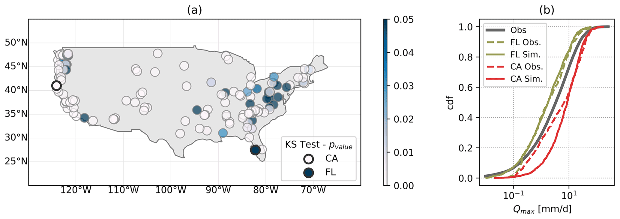
Figure 8 Results from the KS test on the SN-C network. Panel (a) shows the p value of the KS test results at the corresponding catchment location. A p value ≤ 0.05 indicates that H₀ is rejected. Two locations are highlighted: station no. 11481200 in California and station no 02299950 in Florida. Such stations are further analysed in panel (b). Here, the solid grey line indicates the cumulative distribution function modelling the Q_max node in the SN-C network. The red lines represent the observed (dashed) and simulated (solid line) Q_max distribution at the catchment in California. The green lines represent the observed (dashed line) and simulated (solid line) Q_max distribution at the catchment in Florida. The comparison of the coloured lines with the grey line shows that by conditioning on catchments' attributes, the SN-C network returns discharge values in the range of the discharge observable at the catchment. The comparison between solid and dashed lines of the same colour indicates whether conditioning on attributes is sufficient for a good discharge estimation. In Florida the model performs well (the two lines overlap), while in California the model cannot reproduce low quantiles well.

We note that removing one station from the overall pool of observations has a very small effect on the empirical correlation matrix of the empirical variables, the correlation matrix associated with the network, and the cumulative distribution of each node: the observations belonging to one catchment are around 0.8 % of the total observations from all the catchments. This shows that the SN-C network is quite robust. Hence, we further evaluate the robustness of the SN-C network performances as a predictive model by leave-one-out cross-validation. The KS test is performed for each catchment using the value of maximum daily river discharge observed and simulated via the SN-C network, calibrated without the information of the catchment analysed (evaluation process). This is done to assess the potential of such a network in exploiting the information from catchments with similar attributes. The descriptive and the predictive models perform similarly, suggesting that the SN-C network is quite robust. The KS test results show that in only 15 % of the subsample of catchments analysed here (Fig. 8a green dots; 10 % of the total number of catchments), the H₀ cannot be rejected (p value 0.20), meaning that in only 15 % of the catchments, the distribution of simulated and observed Q_max belongs to the same distribution family. Such catchments are characterised by a relatively strong correlation between P_max and Q_max (median around 0.53) and are in energy-limited regions (aridity median ∼0.74) at moderate elevations (median ∼500 m a.s.l.). Moreover, in such catchments, precipitation is on average constant over the year (p_s 0.08). However, there is no clear pattern in catchment attributes of those catchments with H₀ rejected in the predictive model but not rejected in the descriptive model.

To further analyse the results, we look at one catchment in California (no. 11481200), where the H₀ is rejected, and one in Florida (no. 02299950), where the H₀ cannot be rejected. Figure 8b shows that conditioning the SN-C network on catchments' attributes leads to a subsample of discharge values in the range of the observed ones. However, low quantiles are not well captured (dashed coloured lines departing from the corresponding solid lines in Fig. 8b), especially in the catchment in California (red line).

6 Discussion and challenges

The performances of NPBNs indicate that the interdependence between hydro-meteorological information should be explicitly modelled to better capture the river discharge characteristics at the catchment level: the SN-1 network provides higher NSE values compared to the UN-1 network. Additionally, it suggests that at least the networks trained at the catchment scale, i.e. SN-1 and UN-1, show potential to describe the hydrological response, while more research will be needed to develop meaningful NPBNs trained across a range of multiple catchments. Indeed, in our study, river discharge could only be poorly captured by this network type, i.e. SN-C, which reflects the common issue of information transfer in hydrological modelling.

By further considering the results just obtained we identify six issues related to both NPBN properties (i.e. data quality and quantity, independence of weather events, feasibility of testing procedure, and Gaussian-copula assumption) and the river discharge generating process (i.e. catchment heterogeneity, and interacting spatial and temporal scales) that we believe have influenced the networks' performances. We discuss these issues in details, and, when possible, we propose a way to address them.

• Catchment heterogeneity. River discharge generation is the result of underlying physical processes at different timescales, and it occurs in catchments with spatially heterogeneous characteristics. Such complexity affects the performances of a fixed model configuration (i.e. network nodes and interdependence, as summarised by arcs) in which the timescale of the different processes involved is implicitly treated.

• Data quality and quantity. NPBNs, similarly to other models, are sensitive to the quantity and quality of the data used for network quantification. In a NPBN, hydro-meteorological observations and catchment attributes are modelled as random variables, via a parametric (or empirical) distribution function learned from the data themselves. This requires that (for static models) observations used in the training process are also representative of future inference; i.e. they have time-invariant statistics. Such statistics are quite sensitive to the quantity and quality (measurement errors) of the data. This is particularly relevant when modelling extremes, both low and high, since observations of these are already scarce. The results obtained in this study reflect to some extent such difficulty. For example, the SN-1 network for modelling a catchment as single elements over- and underestimates the 5th and the 95th percentile respectively (Fig. 5e, f).

• Interacting spatial and temporal scales. River discharge at the outlet of a catchment is generated from the interaction between many, partially simultaneously occurring physical processes, such as direct runoff, infiltration, and evaporation. These processes are characterised by different spatial and temporal scales and can vary substantially within and across catchments. Specifically, as tested here, in a NPBN the causal relationship between river discharge and hydro-meteorological variables is modelled via (conditional) correlation, which, however, is a measure of dependence and does not imply causation. Therefore, to model the temporal component of the underlying physical processes, we sampled hydro-meteorological variables within a 7 d time window prior to the maximum discharge event. However, with this procedure we might have missed some relevant interaction, such as the different response of river discharge to a precipitation event due to soil conditions. In this regard, further analysis, for example, on how to account more explicitly for soil moisture content (after a preliminary analysis not shown here using ESA CCI products, we only considered monthly runoff coefficient) could improve the results. Our preliminary assessment (results are not shown here) is that there are not enough available remote sensing soil moisture data to provide a representative multivariate data set because of high amounts of missing data, especially over the winter season. Furthermore, the variability of soil moisture content is much higher than discharge, for example, in response to a precipitation event. This is also due to the fact that soil moisture is more sensitive to other input variables, such as temperature, compared to river discharge. Hence, it is challenging to identify at which time frame (i.e. maximum/mean over week/day) information on soil moisture is relevant for improving maximum daily river discharge in any given month.

• Independence of weather events. NPBNs are graphical models to construct a joint distribution function on a given set of random variables represented as nodes in a DAG. At a monthly timescale, the temporal scale considered in this study, samples used in the quantification process are not always time-independent. The sampling procedure of the multivariate data set based on maximum daily events contributes to guaranteeing the time-independence property of the events sampled, since events should be driven by different weather systems. However, some autocorrelation, particularly in discharge data, was observed (Fig. S3). To address this, future research exploring dynamic non-parametric Bayesian networks is recommended Hanea et al. (2013).

• Feasibility of testing procedure. BN model selection is a challenging task due to the high number of possible DAG configurations determining a multivariate probability function describing a given set of variables, where each configuration is de facto a possible hypothesis on the system functioning and may in principle be tested. Furthermore, the same DAG can be quantified differently based on the ordering of the parent nodes. NPBNs specify the nodes as arbitrary invertible distribution functions and the arcs as (conditional) rank correlation (Kurowicka and Cooke, 2005). The conditional correlation depends on the parent ordering chosen for a given child (node). For example, the network in Fig. 3 can be quantified by two pairs of (conditional) rank correlations: r_1,3 and $r_{\mathrm{2},\mathrm{3}|\mathrm{1}}$ or r_2, 3 and $r_{\mathrm{1},\mathrm{3}|\mathrm{2}}$. In the former case, the parent order is {1, 2} and in the latter {2, 1}. In general, given n nodes, the saturated DAG (all the nodes connected) has nⁿ⁻² possible parent–child combinations (Morales-Nápoles, 2010), and this number increases when testing other DAG configurations justified by prior information. This large number of potential models would render network selection on the bases of a “brute force” procedure (evaluating a large portion of the space of models) computationally unfeasible. For such a reason, we imposed the network configuration based on prior knowledge about the relationship between the variables, and we investigated model performances based on the model outcome. This strategy, however, can affect the capability of the model as a catchment descriptor and can conceal relationships that may seem illogical or unlikely a priori. Hydrological applications require a good knowledge of the interactions and dependencies in a system, which are often largely unknown beyond individual catchments, and this is reflected in the fact that in this study, NPBNs, which require information to model dependence, perform better for catchments as single elements than for catchments in a cluster.

• Gaussian-copula assumption. NPBNs, introduced by Kurowicka and Cooke (2005) and implemented in this study, assume that the arcs are quantified via the normal or Gaussian copula (Nelsen, 2006) because only this copula allows for rapid calculation and inference for complex problems (Hanea et al., 2015). However, the normal copula does not capture important asymmetries often observed in data (for example, lower and upper tail dependence), meaning that it is not able to properly model relationships where extreme values (minimum and/or maximum values) are more strongly associated than values not in the joint tails of the distribution. This issue can be solved by quantifying the arcs based on a different copula family. In this way, the join distribution function of the nodes in the network is realised via vine copulas. However, a complete theory of vine copula conditionalisation does not exist, making the process at the least computationally demanding and consequently preventing their applicability to high-dimensional studies such this one.

7 Conclusions

The main objective of this study was to further explore and test the suitability of NPBNs as a tool to reproduce catchment-scale hydrological dynamics and to explore challenges involved when inferring maximum daily discharge, since applications of NPBNs in hydrology are still limited. In this study, we investigated 240 catchments across the United States, obtained from the CAMELS data set, aiming at testing the ability of NPBNs to estimate maximum daily river discharge. We showed that, once a NPBN is defined, it is straightforward to infer any of its variables, i.e. discharge, when the remaining variables are known and extend the network itself with additional variables, i.e. going from the SN-1 network containing only hydro-meteorological variables to the SN-C network containing hydro-meteorological variables and catchments' attributes. The NPBNs individually trained to specific catchments showed potential to reproduce maximum daily river discharge in a wide range of environments with an average NSE of 0.59 (predictive models), while in the literature the performances of regression models for average monthly river discharge showed NSEs ∼0.6 to ∼0.8 (Ren et al., 2020), and the performances for daily river discharge showed NSEs of ∼0.603 and ∼0.598 for the LSTM network and SAC-SMA model respectively (Kratzert et al., 2019). On the other hand, the SN-C network trained across sets of many contrasting catchments exhibited modest skill, i.e. only 10 % of the catchments with an average KS test p value of 0.20. This calls for additional analyses to overcome the limitations encountered and discussed in the previous section to support future studies using statistical-based models. Future research directions will focus on improving the understanding of the timescale at which the many hydro-meteorological variables leading to discharge generation interact. For this purpose, we recommend investigating the potential of dynamic BNs to explicitly model the “memory” of the system (i.e. autocorrelation in the variables). Another research direction is exploring vine copulas to better capture the possible asymmetries observed in extremes.