the Creative Commons Attribution 4.0 License.
the Creative Commons Attribution 4.0 License.
 | 15 Mar 2022
Information content of soil hydrology in a west Amazon watershed as informed by GRACE
Elias C. Massoud
A. Anthony Bloom
Marcos Longo
John T. Reager
Paul A. Levine
John R. Worden
The seasonal-to-decadal terrestrial water balance on river basin scales depends on several well-characterized but uncertain soil physical processes, including soil moisture, plant available water, rooting depth, and recharge to lower soil layers. Reducing uncertainties in these quantities using observations is a key step toward improving the data fidelity and skill of land surface models. In this study, we quantitatively characterize the capability of Gravity Recovery and Climate Experiment (NASA-GRACE) measurements – a key constraint on total water storage (TWS) – to inform and constrain these processes. We use a reduced-complexity physically based model capable of simulating the hydrologic cycle, and we apply Bayesian inference on the model parameters using a Markov chain Monte Carlo algorithm, to minimize mismatches between model-simulated and GRACE-observed TWS anomalies. Based on the prior and posterior model parameter distributions, we further quantify information gain with regard to terrestrial water states, associated fluxes, and time-invariant process parameters. We show that the data-constrained terrestrial water storage model can capture basic physics of the hydrologic cycle for a watershed in the western Amazon during the period January 2003 through December 2012, with an r2 of 0.98 and root mean square error of 30.99 mm between observed and simulated TWS. Furthermore, we show a reduction of uncertainty in many of the parameters and state variables, ranging from a 2 % reduction in uncertainty for the porosity parameter to an 85 % reduction for the rooting depth parameter. The annual and interannual variability of the system are also simulated accurately, with the model simulations capturing the impacts of the 2005–2006 and 2010–2011 South American droughts. The results shown here suggest the potential of using gravimetric observations of TWS to identify and constrain key parameters in soil hydrologic models.
- Article
(7352 KB) - Full-text XML
-
Supplement
(5704 KB) - BibTeX
- EndNote


The terrestrial water balance depends on many physical processes, including soil moisture, plant available water (PAW), rooting depth, recharge to lower soil layers, among others, and these processes depend on each other in a dynamic way (Margulis et al., 2006; Massoud et al., 2019a, 2020a). Some variables, such as precipitation, surface runoff, or soil moisture, can be directly observed in the field or by airborne measurements (Walker et al., 2004; Swenson et al., 2006; Durand et al., 2009; Liu et al., 2019), but other processes, such as evapotranspiration (ET) or groundwater storage changes, are more difficult to detect and observe (Tapley et al., 2004; Pascolini-Campbell et al., 2020). Model simulations are one tool that can be used to fill gaps where our understanding of the hydrologic cycle is incomplete or missing (Purdy et al., 2018; Massoud et al., 2018a). Different types of models exist, such as distributed models with dozens or hundreds of parameters that simulate process-based physics on the grid scale but are extremely expensive to run (Vivoni et al., 2007; Hanson et al., 2012; Longo et al., 2019; Massoud et al., 2019b), or lumped models that aggregate information in space and time to reduce the cost of model simulations while maintaining accuracy compared with measurements (Manfreda et al., 2018; Massoud et al., 2018b). Recent advances in model-data fusion have paved the way to merge land model simulations with observations (Girotto et al., 2016; Khaki et al., 2017, 2018; Quetin et al., 2020; Sawada, 2020), limiting the need for process representation in the model and increasing the efficiency in the inference of unknown physical processes, such as hydrologic variables that cannot be directly measured.
The wealth of data available today, including in situ measurements, flux towers, or satellite data from remote sensing, has made it increasingly possible to fuse model simulations with observations. This has been shown in several works in the literature so far (Massoud et al., 2018a, b; Seo and Lee, 2020). One set of satellite observations that has been very popular in the literature is the NASA Gravity Recovery and Climate Experiment (GRACE) pair of satellites (Tapley et al., 2004). Satellite observations of Earth's gravity field from GRACE are processed routinely into estimates of surface mass change and can provide information about basin-scale dynamics of hydrologic processes. GRACE mass change estimates can be combined with other hydrologic information, such as model simulations or in situ observations, to infer hydrologic parameters and state variables (Famiglietti et al., 2011; Xiao et al., 2017; Trautmann et al., 2018; Massoud et al., 2018a, 2020a; Liu et al., 2019). Numerous studies in the literature have assimilated information from GRACE into models for a better understanding of how groundwater systems behave on different scales (Zaitchik et al., 2008; Houburg et al., 2012; Reager et al., 2015).
Across a variety of climate and land surface models (Christoffersen et al., 2016; Purdy et al., 2018; Massoud et al., 2019a; Schmidt-Walter et al., 2020), hydrology process parameters – both physical states and empirical process variables – constitute a major uncertainty in models. Uncertain variables include rooting depth, infiltration rates, water retention curves, among other soil physical processes, which are governing factors in the dynamic evolution of soil water states. Typically, models prescribe these parameters either by default values or by calibrating the models in well-studied and extensively measured domains. However, few efforts have been made to assess uncertainties tied to the choice of these parameter values. Many of these prescribed parameters come from observational studies, such as Hodnett and Tomasella (2002) and those indicated in Marthews et al. (2014). Studies such as these optimize parameters, along with their dependence on soil characteristics, to represent field measurements of water retention curves. However, the samples are often restricted to a few sites and not necessarily representative of larger regions. Furthermore, the models may have limitations in their physical process representation, which could induce bias in predictions if these parameters are used as the “truth”. In general, information on parameters can be inferred with high confidence using datasets obtained from remote sensing.
In this study, we demonstrate the ability of the decadal GRACE total water storage (TWS) record to inform and reduce uncertainties of terrestrial hydrologic processes regulating the seasonal and inter-annual variability of TWS in the western Amazon, the Gavião watershed, for the period January 2003 through December 2012. To achieve this, we use a model of necessary complexity to represent the first-order controls on seasonal-to-decadal soil moisture dynamics, including soil moisture, soil water potential, PAW, and rooting depth. To characterize and quantify information content of the GRACE record, we employ a Bayesian model-data fusion approach to constrain model parameters (namely initial states and time-invariant process variables), such that differences between GRACE and simulated TWS anomalies are statistically minimized. We henceforth collectively refer to time-invariant parameters governing soil moisture states – such as porosity, rooting depth and hydraulic conductivity coefficients – as model process parameters throughout the manuscript.
Our study is set up as follows. In Sect. 2 we describe the TWS model, the GRACE TWS data used to constrain our simulations, and the Bayesian method used to infer the model parameters. In Sect. 3, we define the model's physically based equations, introduce the time-invariant model parameters that are optimized and inferred, and highlight our findings and results. We summarize our work in Sect. 4 and discuss the implications of our results and priority points for further developments.
2.1 Data-constrained terrestrial water storage model
We employ a model of necessary complexity to represent basin scale hydrologic processes that regulate the storage and movement of water on monthly timescales, as shown in Fig. 1. The model includes two soil layers, where the top layer represents the water that is available to plants via roots (PAW), and the bottom layer representing depths of the soil that plant roots cannot access (plant unavailable water, or PUW). The model uses monthly time steps to integrate the state variables and is driven with hydrologic flux variables such as ET and precipitation. The model also includes other processes such as infiltration into the soil, surface runoff, drainage from each layer, recharge into the lower soil layer, and various model parameters (listed in Table 1) that control the simulations.
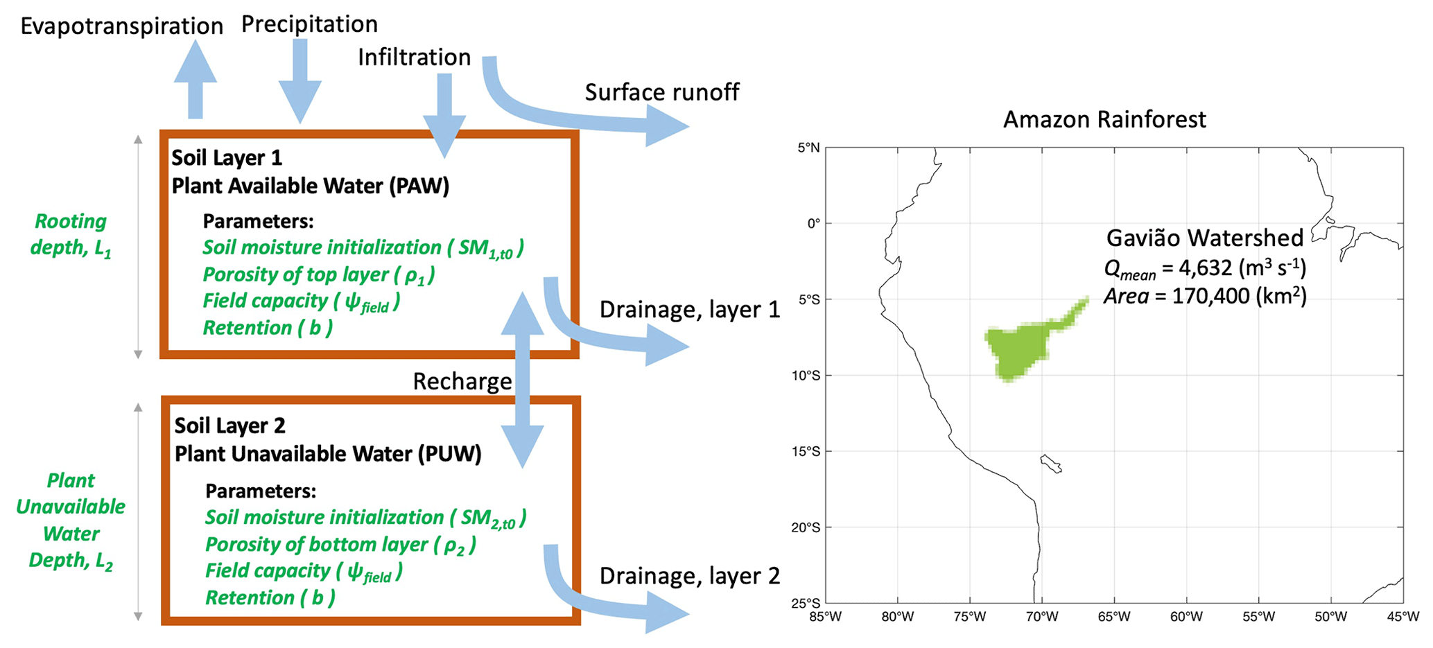
Figure 1Model schematic for the data-constrained terrestrial water storage model. Arrows indicate the logical flow that describes the movement and storage of water in the model. The domain on the right highlights the western Amazonian watershed investigated in this study, the Gavião watershed.
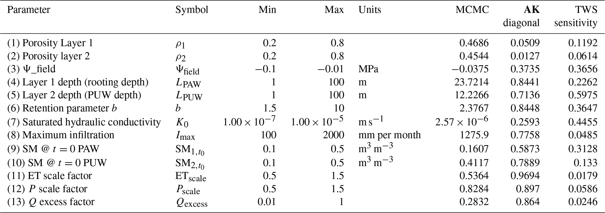
Table 1Parameter estimation results for the Gavião watershed. Shown here are the model parameters and associated symbols, prior ranges (min–max), units, posterior solution median estimate (Markov chain Monte Carlo, MCMC), AK matrix diagonal values showing the level of uncertainty reduction (i.e., AK=1 for full reduction, AK=0 for no reduction in uncertainty), and TWS sensitivities ([mm change in TWS per 1 %-unit change in parameter]) showing the sensitivity of TWS variability to model parameters.
The model includes 13 parameters that represent process-based hydrologic mechanisms, ones that are hypothesized to be influential on basin-scale monthly resolution model simulations of the hydrologic cycle. As depicted in Fig. 1, there are two soil layers representing the PAW and PUW pools. Each of the two separate soil layers has its own inferred physical properties, such as the depth of each layer, soil moisture initialization, porosity, field capacity, and retention capabilities. Various fluxes are represented in the model, such as precipitation (P), evapotranspiration (ET), infiltration, surface runoff, and drainage. The parameters of the model dictate the simulation of each process in the hydrologic cycle, and by adding the two water pools (PAW + PUW), an estimate of total water storage (TWS) can be generated, which can then ultimately be compared with the GRACE-based TWS.
We describe here the model equations that dictate how the TWS is calculated in the model. To start, we know from the water mass continuity that the changes in TWS in the soil is equivalent to the balance between input (precipitation, P) and outputs (ET, and the total loss through drainage and runoff Q). In effect, P and ET are prescribed boundary conditions for the model. In this version of the model,
where represents the PAW and is the PUW each month, t. The soil is represented this way in the model because plants cannot access all the water stored in the ground; therefore, two separate layers are used to represent the soil water in the rooting zone (PAW) and the soil water that is not accessible to plants (PUW).
The following model equations are used to represent the storage and flow of water in the model. The mass continuity equations for water stored in the MPAW and MPUW layers are:
where It is the infiltration into the top soil layer, Dt,PAW and Dt,PUW are the drainage terms for each layer, Ft is the recharge in between layers, and ETt is the ET term each month, t. We assume that a fraction of precipitation cannot infiltrate the soil. This occurs because during rainy events, the precipitation rates often exceed the percolation rates of the near-surface soil, which may become temporarily saturated. These processes occur on sub-monthly scales and cannot be explicitly accounted for in the model; therefore, we use a phenomenological approach that assumes a maximum infiltration rate:
where Pt represents the precipitation rate each month and Imax is the parameter that represents the maximum infiltration. The excess precipitation is lost as surface runoff (St) and never enters the soil storage:
The recharge flux between the PAW and PUW layers (Ft, positive when the flow goes from PAW to PUW) can be defined by Darcy's law, relating the difference in potentials between the two layers:
where Ψt,PAW and Ψt,PUW [MPa] are the soil matric potential of each layer each month, ρl=1000 kg m−3 is the water density, g=9.807 m s−2 is the gravity acceleration, Kt,layer [m s−1] is the hydraulic conductivity of the source layer (i.e., PAW if Fi is positive, and PUW if Fi is negative), and LPUW (rooting depth) and LPAW (remainder of soil depth) are the parameters that represent the thickness of each layer [m].
Then, the soil matric potential of each layer is defined as a function of relative soil moisture (SMt,layer), following Brooks and Corey (1964):
where MPa, and the parameter b corresponds to the inverse of the pore size distribution index (Marthews et al., 2014). The unsaturated hydraulic conductivity (Kt,layer) is defined following Campbell (1974):
where K0 [m s−1] is the parameter that represents the saturated hydraulic conductivity, and the parameter b is the same as in Eq. (7). The drainage function is parameterized as the removal of water that exceeds the field capacity, to represent fast (sub-monthly) loss of water under near-saturated conditions:
where the scaling term Qexcess is a free parameter from 0–1 that removes a fraction of SM excess above field capacity, ψfield.
Last, one thing to note is that precipitation and ET biases in the Amazon are known to be significant, and ET can even have an inverted seasonal cycle. The model is capable of substantially relaxing and constraining the simulated evapotranspiration (ETt) and precipitation (Pt) values each month, through the parameterization and inference of scale factors (Pscale and ETscale). The data set used for P each month, namely Pdata,t, is derived from precipitation measurements from the Tropical Rainfall Measuring Mission (TRMM) 3B42 (Huffman et al., 2007), provided at and 3-hourly spatiotemporal resolutions. The data sets used for ET each month, namely ETdata,t, is derived following the approach in Swann and Koven (2017) and Shi et al. (2019). That is, monthly total ET is derived from satellite observations of precipitation and TWS and ground-based measurements of river runoff. Unlike the ET retrievals from the Moderate Resolution Imaging Spectroradiometer, which have been shown to be seasonally biased in the wet tropics (Maeda et al., 2017; Swann and Koven, 2017), this ET estimation is robust across seasons (Swann and Koven, 2017). Runoff data sets for each watershed are obtained from the Observation Service for the geodynamic, hydrologic, and biogeochemical control of erosion/alteration and material transport in the Amazon (SO-HYBAM) in situ river gauge discharge measurements (discharge measurements can be found at http://www.ore-hybam.org/, last access: 21 March 2017). With these three data sets, we estimate subbasin-based monthly ET.
To clarify this further, three different derivations are used for the TWS variable. These three estimates provide a sense of uncertainty for the TWS. The uncertainty from the GRACE product is used in the likelihood function of the MCMC algorithm when fitting the model-simulated TWS to the GRACE derived TWS. Next, three products are also used in the precipitation and the runoff driving variables that were used, to get a sense of the uncertainty in each variable. To estimate the ET driving variable in this work, we use the mean of the TWS, P, and Q products and create a water balance that will allow us to estimate a mean for the ET driving variable. Then, by application of the ET scaling parameter, we try to estimate whether our initial calculation of ET required any scaling to match the data. Therefore, even though the GRACE TWS is somehow used in the derivation of the ET data, the uncertainty that is applied throughout the work allows us to still estimate ET that is not dependent on the GRACE data. See Shi et al. (2019) for more details on this derivation. In essence, the simulated fluxes are represented as for ET, and for precipitation, where ETscale and Pscale are inferable parameters. Combining all these equations in the logical flow presented in Fig. 1 of the manuscript allows the model to simulate total water storage as . To our knowledge, this model has not been presented before in the literature, and this manuscript is the first to report on the model simulation results.
The parameters of the model will be inferred such that the TWS in the model simulations match the observed GRACE TWS data. As GRACE TWS is known to have the smallest uncertainties in the water budget (see Pascolini-Campbell et al., 2020), we use this information to infer and understand the more poorly constrained variables or processes in the model. In this case study, we use the model for the Gavião watershed, located in the western Amazon (for the location of the watershed refer to the map in Fig. 1). We chose the Gavião watershed for this study owing to sufficient data availability, and because there is a strong seasonal cycle for this watershed, which allows the model to capture hydrologic signals more efficiently during the parameter inference.
2.2 GRACE data for total water storage
The GRACE mission by NASA (Tapley et al., 2004) has proven to be an extremely valuable tool for regional to global scale water cycle studies (Famiglietti, 2014; Reager et al., 2015; Massoud et al., 2018a, 2020a). GRACE data have been widely used to diagnose patterns of hydrological variability (Seo et al., 2010; Rodell et al., 2009; Ramillien et al., 2006; Feng et al., 2013), to validate and improve model simulations (Döll et al., 2014; Güntner, 2008; Werth and Güntner, 2010; Chen et al., 2017; Eicker et al., 2014; Girotto et al., 2016; Schellekens et al., 2017), to constrain decadal predictions of groundwater storage (Massoud et al., 2018a), and to enhance our understanding of the water cycle on regional to global scales (Syed et al., 2009; Felfelani et al., 2017; Massoud et al., 2020a). TWS estimates from GRACE include all of the snow, ice, surface water, soil water, canopy water, and groundwater in a region, and when combined with auxiliary hydrologic datasets, TWS can be utilized to infer process information on model parameters or other model states.
Various recent studies have demonstrated that GRACE-derived estimates of variations of TWS can provide freshwater availability estimates with sufficient accuracy (Yeh et al., 2006; Zaitchik et al., 2008; Massoud et al., 2018a). These GRACE-based methods have been applied to regions such as Northern India (Rodell et al., 2009; Tiwari et al., 2009), the Middle East (Voss et al., 2013; Forootan et al., 2014; Massoud et al., 2021), Northern China (Moiwo et al., 2009; Feng et al., 2013), California (Famiglietti et al., 2011; Scanlon et al., 2012; Xiao et al., 2017; Massoud et al., 2018a, 2020a), northern mid- to high latitudes (Trautmann et al., 2018), and the Amazon (Swann and Koven, 2017). In this study, estimates of TWS are obtained from the GRACE retrievals of equivalent water thickness (Landerer and Swenson, 2012; Sakumura et al., 2014; Wiese et al., 2016). We use three GRACE TWS retrievals from the spherical harmonic data versions generated by the Center for Space Research (CSR), GeoforschungsZentrum Potsdam (GFZ), and Jet Propulsion Laboratory (JPL). These three GRACE TWS retrievals are 1-degree solutions of land field products (each was downloaded from ftp://podaac-ftp.jpl.nasa.gov/allData/tellus/L3/land_mass/RL05/, last access: 14 June 2017). We calculate the arithmetic mean of the three GRACE TWS retrievals to represent TWS used in Eq. (1). We used this GRACE product to constrain simulations of the hydrologic model described in Sect. 2.1 for the Gavião watershed from January 2003 through December 2012.
2.3 Bayesian parameter inference with MCMC
In this study, we aim to estimate parameters of a medium complexity model that simulates the hydrologic cycle using physics-based equations that capture large scale dynamics of the watershed. We showcase how the data-constrained, physically based model can simulate the hydrologic cycle by fusing the model with auxiliary observations. When simulated on its own, the model can represent a wide range of physical possibilities, but when calibrated and trained to fit some desired observed metric, the model simulations begin to represent the underlying physical system it is being trained to. Many tools exist to achieve model-data fusion, such as Bayesian parameter inference with MCMC algorithms (Schoups and Vrugt, 2010; Bloom et al., 2015; Vrugt, 2016; Vrugt and Massoud, 2018; Massoud et al., 2019c, 2020b) or data assimilation (Reichle et al., 2002; Vrugt et al., 2005; Girotto et al., 2016; Khaki et al., 2017, 2018; Massoud et al., 2018b). These state-of-the-art tools require enough computational cost but can ensure that the underlying system dynamics are being accurately replicated to an agreeable amount of uncertainty. The model parameters in this study are estimated using Bayesian inference with MCMC (Vrugt and Massoud, 2018), where the final estimated distributions are not required to follow any form, such as Gaussian or bimodal. The final estimates of the model parameters, shown later to be the posterior of θ in Eq. (12), are the posterior solutions and are utilized to constrain the spread of uncertainty in the simulations.
In recent decades, Bayesian inference has emerged as a working paradigm for modern probability theory, parameter and state estimation, model selection, and hypothesis testing (Vrugt and Massoud, 2018). According to Bayes' theorem, the posterior parameter distributions, P(A|B), depend upon the prior distributions, P(A), which captures our initial beliefs about the values of the model parameters, and a likelihood function, L(θ), which quantifies the confidence in the model parameters, θ, considering the observed data, Y. The likelihood function is a critical property of this calculation. This section shows the derivation of the likelihood function used in this study. According to Bayes' Theorem, the probability of an event is estimated based on prior knowledge of conditions that might be related to the event. In equation form, this looks like:
For the purposes of this study, we can express P(A) as the prior information of our calculation, which assumes that log-uniform distribution for all parameters and the probability outside the parameter bounds is equal to 0 (the minimum and maximum values for each parameter are reported in Table 1). P(B) is the evidence and is a normalizing constant and therefore taken out of the equation. This leaves us with:
where P(A|B) is the final distribution of the model parameters, or the posterior of θ in Eq. (12) described in the next paragraph, and P(B|A) is equivalent to the chosen likelihood function, L(θ), also described in the next paragraph. Therefore, the MCMC algorithm samples model parameter combinations (θ) that will maximize the fit to the GRACE data, and thus will maximize the value of the likelihood function, L(θ).
The observed data in this case study is the GRACE satellite observations, and our goal is to find the optimal set of model parameters, θ, that produces a model simulation, X(θ), which maximizes the fit, or the likelihood, relative to the observations. Our likelihood function is therefore set up as:
where t refers to the time index (in months) of the simulations, YGRACE,t is the observed GRACE data at month t, XModel,t(θ) is the optimized model simulations at month t using the parameters θ, and is the uncertainty associated with the GRACE data, which was chosen to be a homogeneous 50 mm per month for our applications. As GRACE data are represented as anomalies from climatology, we format the model simulations into anomalies as well to perform this model-data-fitting experiment. That is:
indicating that the form of the GRACE observations is in climatological anomalies. Furthermore, we format the model simulations in this manner for the parameter inference, as follows:
We apply Bayesian inference on the model parameters in an optimization framework and sample the likelihood function in Eq. (12). This allows for the inference of the model parameters, or θ. These inferred model parameters will be used to inform and constrain the spread of uncertainty in the model simulations.
Successful use of the MCMC application in a Bayesian framework depends on many input factors, such as the number of chains, the prior used for the parameters, the number of generations to sample, and the convergence criteria. For our application, we use the adaptive Metropolis-Hastings MCMC, as described in Bloom et al. (2020). We use C=4 chains, the prior was a log-uniform distribution for each parameter and the ranges shown are listed in Table 1, the number of generations was set at G=100 000, and the convergence of the chains relied on the Gelman and Rubin (1992) diagnostic, where we applied the commonly used convergence threshold of R=1.2. Given the high efficiency of running this parsimonious model (compared with other high dimensional and expensive models), it was computationally feasible to obtain the set of G=100 000 simulations for the MCMC algorithm (i.e., less than 1 h of CPU time to perform the parameter inference).
2.4 Averaging kernel matrix
To better quantify the reduction of uncertainty for each parameter, we apply an averaging kernel (AK) calculation (Worden et al., 2004), which is typically a measure of how a modeled state (posterior) is sensitive to changes in the “true” state (prior) and is a method that is common for satellite retrievals. The AK matrix is calculated as follows:
where AK is the diagonal vector of the averaging kernel matrix, I is the identity matrix, “Posterior” is the Bayesian parameter posteriors sampled with MCMC, “Prior” are samples randomly drawn from the prior distribution, and cov is the covariance function. We take the main diagonal of the AK matrix, which represents uncertainty reduction from the prior to the posterior parameter distributions. The AK diagonal values for each parameter are listed in Table 1 under “AK Diagonal”. A value of AK=1 represents a 100 % reduction in uncertainty, whereas a value of AK=0 represents no information gain and therefore no reduction in uncertainty.
3.1 Sensitivity of TWS variability to model parameter
To characterize the sensitivity of the monthly TWS variability to model parameters, we perturb posterior parameters and generate corresponding TWS simulations. Figure 2 shows the sensitivity of the model-simulated TWS to minor perturbations in parameter values. In these plots, the green curves show changes in simulated TWS (dTWS) when each parameter is perturbed (dPar) by 1 % of its prior range, indicating the magnitude and the time steps of model sensitivity. Results in these plots show that sensitivity to initial conditions is higher for the first 12-month period but is diminished after that. Furthermore, the sensitivity of simulated TWS varies between wet and dry seasons.

Figure 2Sensitivity of the model-simulated TWS to minor perturbations in parameter values. Shown here (from top to bottom) are sensitivities to (a) the rooting depth parameter, (b) the maximum infiltration parameter, and (c) the soil moisture initialization parameter for layer 1. Green curves are the changes in simulated TWS (dTWS) when each parameter is perturbed (dPar) by 1 % of its prior range, indicating the magnitude and the time steps of model sensitivity. TWS sensitivities to other parameters are shown in Fig. S3. The x-axis depicts the number of months since 2003, showing the 10-year period starting in January 2003 and ending in December 2012.
The rooting depth parameter (Fig. 2a) is sensitive during initialization as well as during the wet periods, the maximum infiltration parameter (Fig. 2b) seems to only be sensitive during the wet periods, and the parameter representing the initialization of soil moisture in the top layer (Fig. 2c) is only sensitive during initialization. Figure S1 in the Supplement shows how the remaining parameters affect TWS sensitivity. To summarize these curves in a single value (i.e., [mm change in TWS per 1 %-unit change in parameter]), we show in Table 1 under “TWS sensitivity” the aggregated value for each parameter, calculated as the mean variance of all (dTWS/dPar) curves for each parameter.
3.2 Posterior model parameters and simulated states
3.2.1 Model parameters, TWS, and states – the Gavião watershed
We apply Bayesian inference to the model parameters and simulations and optimize the fit to the GRACE data to obtain posterior solutions of the model parameters. We apply this parameter inference for three basins. The first is the Gavião watershed (shown in Fig. 1), which has a generally wet climate. We then perform the same parameter inference to a basin that is wetter than Gavião and is located upstream from the Acanaui river gauge station (hereafter called Basin 1), and to a basin that is drier than Gavião and is upstream from the Guayaramerin river gauge station (hereafter called Basin 2).
For the Gavião watershed, the prior and posterior parameter distributions are shown in Fig. 3, and the median value for these distributions is listed in Table 1 under “MCMC” for each parameter. We investigated how the estimated parameter values we find in this study compare with other studies in the literature. For example, the retention parameter “b” in our study is estimated to be around 2, which is lower than the tabulated values of Cosby et al. (1984), Tomasella and Hodnett (1998), or Marthews et al. (2014). Of course, the model in this study is simulated at much coarser resolution, and the physical meaning of these parameters may change owing to processes being solved on very different scales. This is an important message for the interpretation of these results, as taking a model developed on one scale and applying it to a different scale can induce spurious errors if parameters are not adequately constrained at the intended resolution. We found that most parameters exhibited a significant uncertainty reduction for the Gavião watershed. To quantify this reduction of uncertainty, we apply an averaging kernel (AK) calculation. The results from the AK matrix are listed in Table 1 under “AK diagonal”, and they indicate that significant uncertainty reduction occurs in some parameters, namely the depth of the PAW layer (rooting depth) and the depth of the PUW layer, as well as the retention and maximum infiltration parameters. In contrast, we found that porosity, conductivity at saturation, and ψfield exhibited the smallest relative uncertainty reductions.
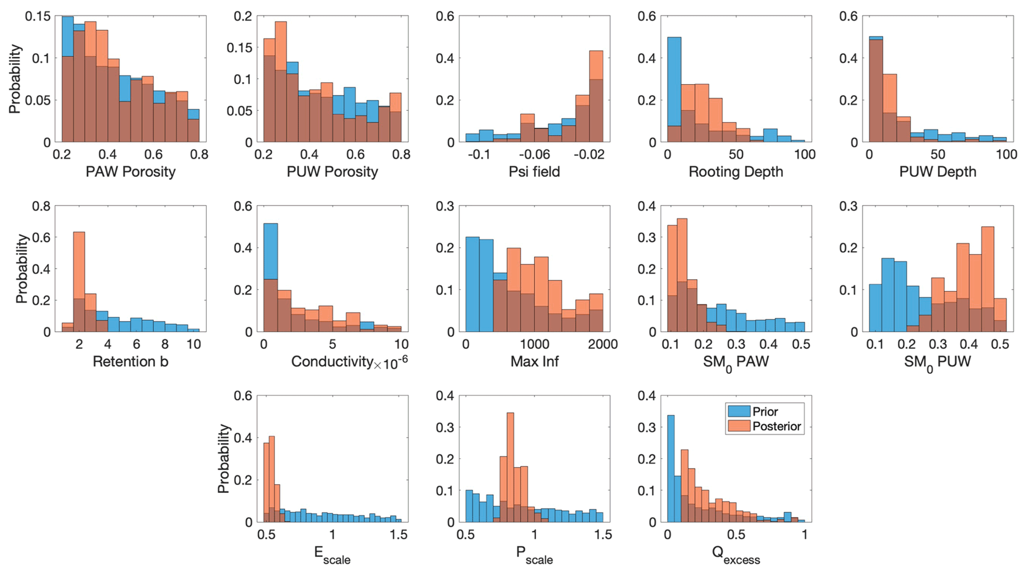
Figure 3Histograms of the prior (blue) and posterior (orange) distributions of the GRACE-informed parameters for the Gavião watershed.
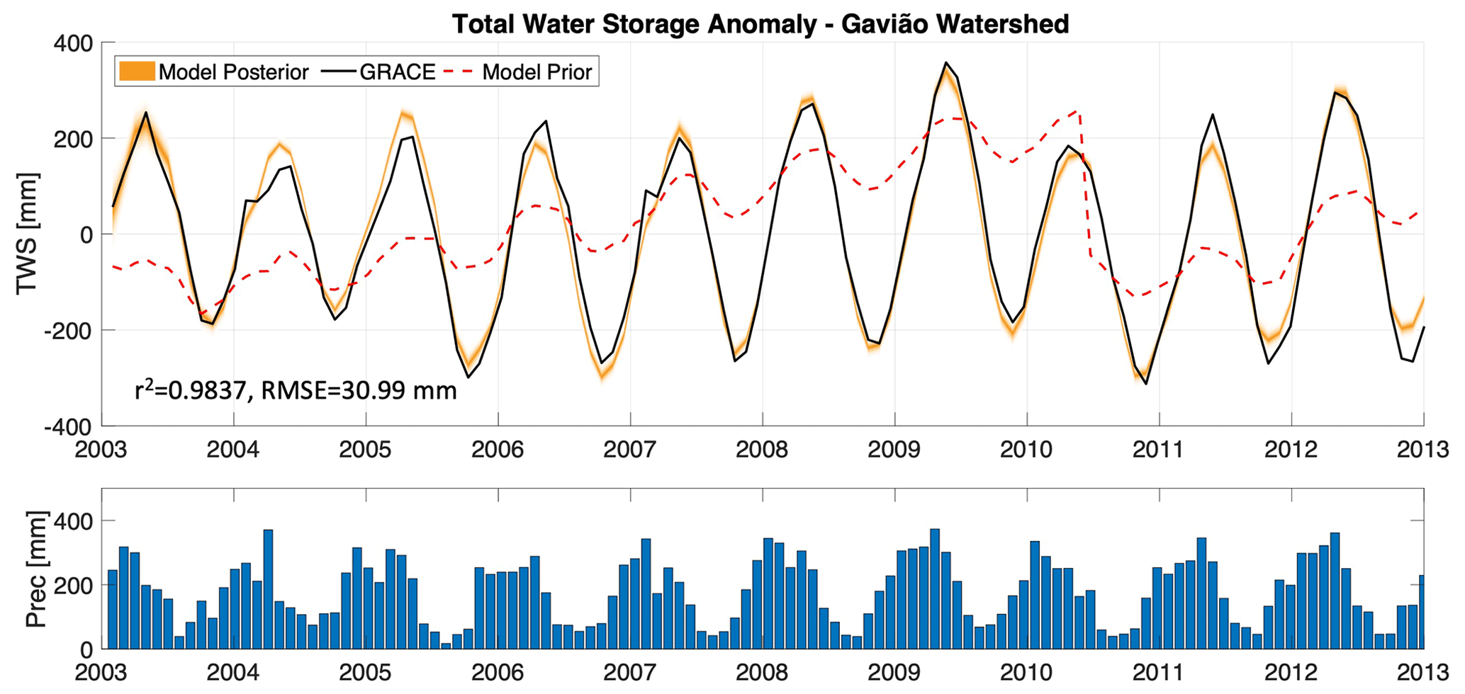
Figure 4Monthly total water storage (TWS) anomaly estimates from satellite data (GRACE TWS), the prior simulation from the model, and the data-constrained version of the model simulations for the Gavião watershed. GRACE-informed posterior ranges of the model-simulated TWS are shown here in the orange envelopes. Precipitation values used to drive the model are shown to indicate the seasonal cycle.
In Fig. 4 we show the model simulations of 10-year monthly TWS for the Gavião watershed, including the prior and the posterior simulations, and compare these with the values obtained from satellite data (GRACE TWS). Posterior ranges of the model-simulated TWS are shown in the orange envelopes, and precipitation values used to drive the model are shown to indicate wet vs dry periods. Results in Fig. 4 show that GRACE-informed soil hydrologic model simulations (posterior) can capture the monthly TWS compared with concurrent GRACE measurements, with an r2=0.9837 and root mean square error (RMSE) = 30.99 mm between observed and simulated TWS. Comparing this result with the prior model simulations (mean of the prior shown in Fig. 4, and the distribution from the prior is shown in Fig. S2), we see a major improvement in the constrained posterior model simulations. The mean prior has an r2=0.4360 and RMSE = 10.50 mm compared with the GRACE TWS, and the range of the prior simulations in Fig. S2 span a wide range of possibilities. This result indicates that this simple model can accurately simulate TWS in the Gavião watershed when the parameters are inferred using GRACE measurements as a fitting target.
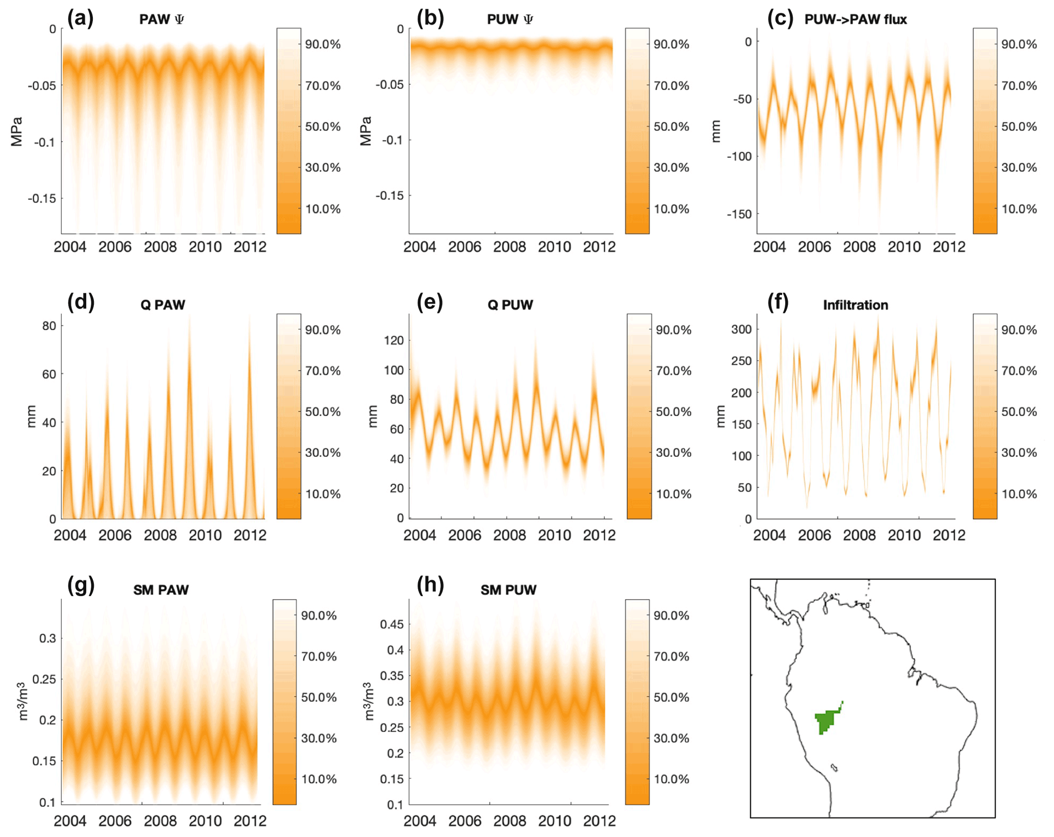
Figure 5GRACE-informed model-simulated states and fluxes for the Gavião watershed (basin shown in the bottom right panel in the context of the broader South American domain). These figures show specific model processes, such as (a) the matric potential of plant available water (PAWψ), (b) the matric potential of plant unavailable water (PUWψ), (c) recharge (PUW-> PAW flux) where negative values indicate a downward flux, (d) discharge from the top layer (QPAW), (e) discharge from the bottom layer (QPUW), (f) infiltration, (g) soil moisture of the top layer (SM PAW), and (h) soil moisture of the bottom layer (SM PUW). The ranges shown here in orange envelopes indicate the GRACE-informed posterior ranges. A map showing the location of the Gavião watershed is shown in the bottom right panel.
The model is then simulated using all samples from the posterior, which provides posterior solutions for the state variables. These are shown in Fig. 5, which displays specific model processes for the Gavião watershed (map of the basin shown in the bottom right panel of Fig. 5). The matric potential of plant available water (PAWψ) and the matric potential of plant unavailable water (PUWψ) represent the suction pressure in each soil layer that is associated with dryness/wetness. In other words, a completely wet soil layer would have a matric potential of 0 and higher levels of dryness result in more negative matric potential values. Based on the results in Fig. 5a and b, the PUW layer seems to have more wetness, and therefore less suction pressure, for this watershed (i.e., values closer to 0 for the PUW layer). The recharge value (PUW-> PAW flux) represents the flux of water from the top layer to the bottom layer, where negative values indicate a downward flux. Results in Fig. 5c show that a flux of water continually flowing downward from the top layer (PAW) to the bottom layer (PUW), roughly at the magnitude of 50–100 mm per month. The discharge values represent the drainage from the top layer (QPAW) and from the bottom layer (QPUW). The results in Fig. 5d and e show that there is drainage from the top layer (PAW) that peaks in the wet season at roughly 40 mm per month, and that there is drainage that follows a seasonal cycle from the bottom layer (PUW) at around 40–80 mm per month. The infiltration represents the water that infiltrates from the surface into the top soil layer. According to Fig. 5f, this flux also follows a seasonal cycle, with about 250 mm per month infiltrated into the top layer during the wet season and dropping to roughly 50 mm per month in the dry season. Last, soil moisture of the top (SM PAW) and bottom layers (SM PUW) represent the state of soil moisture in each layer. Based on the results in Fig. 5g and h, the PUW layer seems to have more wetness, and therefore higher soil moisture values, for this watershed and these results correspond to what is seen for the matric potential in Fig. 5a and b (i.e., more wetness in the PUW layer). In Fig. 5, the ranges shown in orange envelopes are the posterior ranges, indicating the range of possible solutions for each GRACE-informed state variable for the Gavião watershed. Some dynamical constraints were applied in the Bayesian optimization, such as SM and SM, are greater than 0.1 but less than 0.5 [m3 m−3]. The rationale for these “common-sense” rules follows that of Bloom and Williams (2015), to ensure that nonrealistic physical properties of the system are not allowed.
The resulting model simulations are largely affected by the way that ET is used in the model. We described in the methods section how ET is calculated in our study, and it is important to note that there are alternative approaches for prescribing watershed ET. For example, FLUXCOM (Jung et al., 2019), JPL-PT ET (Fisher et al., 2009), or parsimonious prognostic ET scheme (Liu et al., 2021) estimates can provide robust alternatives for the residual-based ET approach.
3.2.2 Interpretation of results
The posterior parameters and model simulations provide information that can be used to identify and estimate the processes responsible for TWS variability in this watershed. Insights into rooting depth (histograms in Fig. 3) are critical for determining the resilience of rootzone water storage during dry season events (see Lewis et al., 2011; Shi et al., 2019; Liu et al., 2017, amongst others). Insights into soil water potential seasonality (posteriors in Fig. 5) are critical for resolving plant hydraulic process responses to atmospheric water demand and soil water supply (Novick et al., 2019; Konings and Gentine, 2017; Liu et al., 2021). Quantitative top-down insights into the infiltration, retention, and runoff parametrizations (histograms in Fig. 3 and posteriors in Fig. 5) are key to understanding the partitioning of precipitation – and its associated seasonal and inter-annual variability – into runoff and storage (which all remain key uncertainties in hydrologic models). Ultimately, mechanistic insights allow for further investigations into instantaneous and lagged responses of soil hydrologic states to climatic variability. Of course, these process dynamics can vary between watersheds, and it is important to understand the causes and drivers of variability in water storage between basins.
3.2.3 Model parameters, TWS, and states – other basins
To ensure that the results from the parameter inference can provide insights into other basins, we estimate parameter posteriors and corresponding TWS simulations for the two other basins mentioned above, Basin 1 (a basin that is wetter than Gavião and is located upstream from the Acanaui river gauge station) and Basin 2 (a basin that is drier than Gavião and is upstream from the Guayaramerin river gauge station). Table S1 in the Supplement reports the median value for the posterior distributions of each parameter in each basin. The TWS simulations for each basin are shown in Fig. S3 (Basin 1) and Fig. S4 (Basin 2). Applying the parameter inference for these basins also produced accurate simulations, with an r2=0.9548 and RMSE = 28.49 mm between observed and simulated TWS for Basin 1 (Fig. S3), and an r2=0.9891 and RMSE = 18.89 mm between observed and simulated TWS for Basin 2 (Fig. S4). Furthermore, we show in Figs. S5 and S6 the GRACE-informed model-simulated states and fluxes for Basins 1 and 2, respectively. From these results, it is apparent that Basin 1 is wetter than Basin 2, e.g., this can be seen by comparing the precipitation levels depicted in Figs. S3 and S4, but also by comparing the matric potential values in panel a or the discharge values in panels d and e in Figs. S5 and S6. The location of these basins in the context of the broader South America are shown in the bottom right panel of Figs. S5 and S6. Overall, the modeled state variables and parameters for these basins are constrained using the GRACE data, and this information can be used to identify and estimate the processes responsible for TWS variability in these watersheds.
3.3 Model simulations at the Gavião watershed: model validation, annual cycle, and annual variability
3.3.1 Model calibration and validation
It is typical in works involving parameter inference to apply a model calibration and a model validation to different periods of the data set to ensure that the estimated parameters are not over-fitting the data and can be used to describe the underlying system and thus make predictions. In this section, we apply a model calibration in the Gavião watershed for the first half of the data set spanning 5 years, and then we apply a validation for the second half of the data set spanning the remaining 5 years. Figure 6 shows results for the model calibration and validation. Posterior ranges of the model-simulated TWS are shown in Fig. 6 in the orange envelopes for the calibration and validation years, and the red line represents the mean estimates for the validation period. The results in Fig. 6 show that the calibration period RMSE is 47.71 mm with a correlation of 0.9520, and for the validation period the RMSE is 40.17 mm with a correlation of 0.9801. This shows that the estimated parameters during the calibration period are still valid for the validation period and indicates that the GRACE-informed soil hydrologic model parameters are both useful for diagnosing present-day soil water dynamics (calibration) as well as predicting seasonal and inter-annual soil water dynamics (validation).

Figure 6Model calibration and validation for monthly TWS anomaly estimates in the Gavião watershed, for the period January 2003 through December 2012. The plot shows the first 5 years of the data for calibration and the remaining 5 years for validation. GRACE-informed posterior ranges of the model-simulated TWS are shown here in the orange envelopes for the calibration and validation years, and the red line is used to represent the mean estimates for the validation period.
3.3.2 Annual cycle and annual variability
We further investigate the ability of the tuned model to capture the annual variability in TWS in the Gavião watershed. In Fig. 7a, we compared the annual cycle of the TWS anomalies produced from GRACE with those produced by the model. The annual variability is captured well with the model, with an r2=0.9979 and RMSE = 11.00 mm between observed and simulated TWS annual cycles. The annual cycle of the mean prior simulation is also shown in Fig. 7 (dashed red line) for comparison. In Fig. 7b, the timeline of de-seasonalized TWS anomaly estimates are shown. To obtain this plot, we subtract the annual cycle in Fig. 7a from each month's estimate shown in Fig. 4. The de-seasonalized plot in Fig. 7b has an r2=0.8512 and RMSE = 29.27 mm between observed and simulated timelines, and the model accurately portrays whether a dry or wet period is experienced relative to what is expected in the annual cycle. This is a vast improvement from estimating the annual cycle and de-seasonalized TWS timeline in the prior simulations (mean prior simulation shown in Fig. 7, and the distribution of prior simulations is shown in Fig. S7). For the prior simulations of the annual cycle, the model has a r2=0.9761 and RMSE = 417.62 mm, and for the de-seasonalized TWS timeline, the model prior has a r2=0.4323 and RMSE = 93.32 mm between observed and simulated timelines. Therefore, the model posterior solutions show a great improvement compared with the prior for simulating the annual cycle and capturing the seasonality of the hydrologic cycle for each watershed.
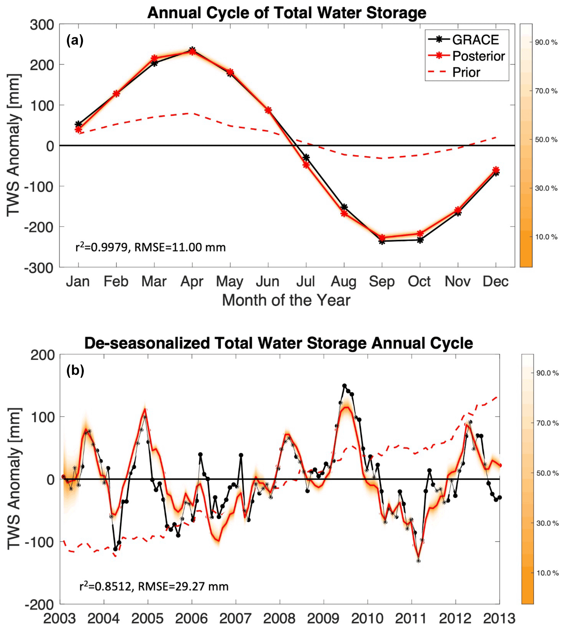
Figure 7(a) Annual cycle of the monthly TWS anomalies [mm], from satellite data (GRACE), the prior simulation from the model (Prior), and the data-constrained version of the model simulations (Posterior) for the Gavião watershed. GRACE-informed posterior ranges of the model-simulated TWS annual cycle are shown here in the orange envelopes. (b) To obtain the de-seasonalized values of TWS for the Gavião watershed shown in panel (b), we subtract the annual cycle in panel (a) from each month's estimate shown in Fig. 4. This shows whether the anomaly values in each time step of panel (b) portrays an extremely dry or wet period relative to what is expected in the annual cycle. Hence, the data-constrained model can capture the 2005–2006 and 2010–2011 droughts that are shown in the GRACE data.
In the results shown in Fig. 7, we see that the model can capture the 2005–2006 and 2010–2011 droughts in the Gavião watershed that are shown in the GRACE data (see Lewis et al., 2011). The model also captures the wet periods observed in 2003, 2004, 2008, 2009, and 2012 (see Fig. 7b). The model captures the positive and negative anomalies quite well; however, it does have some limitation in capturing the magnitude of some extreme events (positive and negative), which may be partly caused by the coarser time step and spatial scale of the simulation. Yet, the model does succeed in capturing some delayed anomalies in water storage following the 2005–2006 and 2010–2011 droughts, which is very promising. This gives confidence in the data-constrained model to provides meaningful estimates of TWS anomalies on monthly and seasonal scales.
3.4 Correlations between posterior model parameters and model states
After the model parameters and states variables are constrained by the GRACE data for the Gavião watershed, relationships between the model parameters and simulated states begin to emerge. We show in Fig. 8a the scatter plot between posterior solutions of model-simulated TWS and the excess runoff parameter. This figure shows that the region inside the black box, or the high-density region of the posterior, is the region within the posterior domain that has high information content (i.e., plausible solutions with a high likelihood). The true value provided by the GRACE data is marked with a red line in Fig. 8a. Other regions of this space, such as locations with excess runoff values below 0.2, produce unlikely model simulations, and similarly, locations with excess runoff values higher than 0.5 are also less likely. This can also be seen in Fig. 3, in the posterior histograms for the excess runoff parameter. Similar relationships between other parameters and state variables (including soil moisture of layer 1 and discharge from layer 1) are shown in Fig. S8. Overall, these plots not only show the emergent relationships between variables as informed by GRACE, but also indicate if and how they correlate in the Gavião watershed.
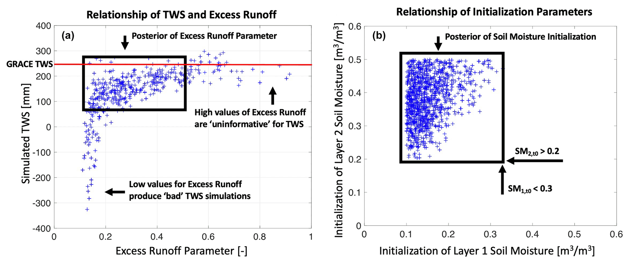
Figure 8(a) Posterior relationship of the model-simulated TWS [mm] during April 2003 and the runoff excess parameter [unitless]. The region inside the black box indicates the posterior region with high density, i.e., plausible solutions with high likelihood. The red line shows the “true” TWS value seen in the GRACE data for this period. (b) Posterior relationship of the initialization parameters for soil moisture in layers 1 and 2, respectively. Initial SM in layer 2 is larger than 0.2 [m3 m−3], initial SM in layer 1 is less than 0.3 [m3 m−3], and SM is generally larger than SM, as indicated in this plot. See Table 1 and Sect. 3.4 for details.
Similarly, the posterior parameter solutions can be used to infer relationships between the parameters themselves. To this end, we show in Fig. 8b a scatter plot depicting the GRACE-informed correlation of the posterior parameter values for the soil moisture initialization parameters in the Gavião watershed. We see that the initial soil moisture in the bottom layer is greater than 0.2 [m3 m−3], and in the top layer it is less than 0.3 [m3 m−3], which can be seen in Fig. 3, in the posterior histograms for the soil moisture initialization parameters. One property that also emerges in Fig. 8b is that the initial soil moisture in the bottom layer is larger than that of the top layer. This indicates that, in the initial time step of the simulations, the bottom layer should have greater soil moisture than the top layer. These relationships can be created for any pair of parameters in the posterior space, and Fig. S9 portrays these relationships for several combinations of parameters, indicating what combinations of parameters are possible for this hydrologic system, as inferred by GRACE.
We summarize the results reported in this subsection with the following points. First, we find considerable correlations between the posteriors of individual model parameters and model states in the Gavião watershed. We also find considerable correlations between the posteriors of individual model parameters and other parameters. This is important, because the correlations between parameters and states indicate that the choice of hydrologic constants can have a considerable impact on simulated TWS. The relationships found in the parameter posteriors imply that although several parameters exhibit considerable uncertainty, only a subset of parameter combinations provide GRACE-consistent model solutions. In essence, these GRACE-based relationships portray what parameter combinations are possible for accurately simulating the chosen watershed.
In this paper we used a parsimonious hydrologic model capable of simulating various aspects of land surface hydrology, and we ran the model for different basins in the western Amazon. We performed extensive analysis on the Gavião watershed, a relatively wet basin, and also reported results for two other basins, one wetter (Basin 1) and one drier (Basin 2). The model used in this study includes two soil layers (plant available and unavailable water pools), is driven by hydrologic flux variables such as ET and precipitation, and includes other processes such as infiltration into the soil, surface runoff, drainage from each layer, and recharge into the lower soil layer. Various model parameters that control the simulations for the Gavião watershed, with their respective estimated values, are listed in Table 1. Table S1 lists these parameter values for Basins 1 and 2. We applied Bayesian inference to estimate posteriors for the model parameters that allowed the simulations to match satellite-based estimates of TWS obtained from GRACE.
Results in this paper showcased the estimated parameter posteriors along with their priors (Fig. 3), the posterior solution of simulated TWS (Fig. 4), and the estimated model states (Fig. 5). We also performed a model calibration and validation exercise (Fig. 6), to show how estimated parameters during the calibration period are still useful for the validation period. We also compared the annual cycle and de-seasonalized TWS anomalies produced from both the GRACE data and the model, and we showed how the data-constrained TWS model can capture the annual variability as well as drought events that occurred in this system (Fig. 7a and b). For further diagnosis of our results, we showed the relationships between model-simulated states and the estimated parameters (Figs. 8a and S8). Then we showed relationships between combinations of estimated parameters (Figs. 8b and S9). Furthermore, we investigated the sensitivity of the model-simulated TWS to minor perturbations in parameter values (Figs. 2 and S1), and we showed how parameters can create sensitivities in TWS in different ways, for example, during wet or dry periods, or during model initialization. Simulation results for Basins 1 and 2 are shown in Figs. S3–S6.
Overall, the results in this paper allowed us to make the following conclusions. First, GRACE-informed soil hydrologic model parameters are useful for diagnosing present-day soil water hydrology. Substantial uncertainty reduction was found for parameters that represent soil moisture initialization, rooting depth, and conductivity and retention relationships. However, limited uncertainty reduction was found for infiltration rates and porosity parameters, and further model development may be needed to describe the information content of these processes and their associated uncertainties more accurately. The second conclusion is that GRACE-informed model parameters can be used for predicting seasonal and inter-annual soil water hydrology. We showed that using a 5-year data record of TWS allows the parameter inference to still be applicable to the remaining 5-year data record, which is simulated without the use of information from GRACE. Last, a medium complexity model like the one used here can be sufficient for capturing monthly to seasonal-scale hydrology of the land surface at the basin scale, such as the Gavião watershed in the Amazon.
By fusing information from the signal of the surface mass change with other hydrologic information, such as physical constraints in model simulations or seasonal behavior of in situ observations, GRACE has proven its ability to infer hydrologic parameters and state variables accurately. We found that this methodology is generalizable to other regions, and we reported the results from additional testing that was conducted on other watersheds in the Amazon. Our results suggest the potential of using gravimetric observations of TWS from GRACE to identify and constrain key parameters in soil hydrologic models.
The codes are available by contacting the authors.
GRACE data are available at https://grace.jpl.nasa.gov/data/get-data/ (NASA, 2022).
The supplement related to this article is available online at: https://doi.org/10.5194/hess-26-1407-2022-supplement.
ECM led the investigation, conceptualized the research, did the formal analysis and model simulations, and wrote the original draft. AAB took responsibility for the investigation, developed the methodology, conceptualized the research, acquired the funding and the resources, and reviewed and edited the paper. ML developed the methodology, conceptualized the research, and reviewed and edited the paper. JTR and PAL reviewed and edited the paper. JRW did the formal analysis, took responsibility for the investigation, reviewed and edited the paper, and supervised the project.
The contact author has declared that neither they nor their co-authors has any competing interests.
Publisher's note: Copernicus Publications remains neutral with regard to jurisdictional claims in published maps and institutional affiliations.
This research was carried out at the Jet Propulsion Laboratory, California Institute of Technology, under a contract with the National Aeronautics and Space Administration. Copyright 2021. A portion of this work was supported by funding from the NASA GRACE-FO Science team. Marcos Longo was supported by the NASA Postdoctoral Program, administered by Universities Space Research Association under contract with NASA. The authors thank Alexandra Konings for insightful discussions that helped to form the concepts presented in this paper.
This research has been supported by the National Aeronautics and Space Administration (grant no. 80NM0018D0004).
This paper was edited by Patricia Saco and reviewed by two anonymous referees.
Bloom, A. A. and Williams, M.: Constraining ecosystem carbon dynamics in a data-limited world: integrating ecological “common sense” in a model–data fusion framework, Biogeosciences, 12, 1299–1315, https://doi.org/10.5194/bg-12-1299-2015, 2015.
Bloom, A. A., Bowman, K. W., Liu, J., Konings, A. G., Worden, J. R., Parazoo, N. C., Meyer, V., Reager, J. T., Worden, H. M., Jiang, Z., Quetin, G. R., Smallman, T. L., Exbrayat, J.-F., Yin, Y., Saatchi, S. S., Williams, M., and Schimel, D. S.: Lagged effects regulate the inter-annual variability of the tropical carbon balance, Biogeosciences, 17, 6393–6422, https://doi.org/10.5194/bg-17-6393-2020, 2020.
Brooks, R. H. and Corey, A. T.: Hydraulic properties of porous media, Hydrology Paper No. 3, Civil Engineering Department, Colorado State University, Fort Collins, CO, 1964.
Campbell, G. S.: A simple method for determining unsaturated conductivity from moisture retention data, Soil Sci., 117, 311–314, 1974.
Chen, X., Long, D., Hong, Y., Zeng, C., and Yan, D.: Improved modeling of snow and glacier melting by a progressive two-stage calibration strategy with GRACE and multisource data: How snow and glacier meltwater contributes to the runoff of the Upper Brahmaputra River basin?, Water Resour. Res., 53, 2431–2466, https://doi.org/10.1002/2016WR019656, 2017.
Christoffersen, B. O., Gloor, M., Fauset, S., Fyllas, N. M., Galbraith, D. R., Baker, T. R., Kruijt, B., Rowland, L., Fisher, R. A., Binks, O. J., Sevanto, S., Xu, C., Jansen, S., Choat, B., Mencuccini, M., McDowell, N. G., and Meir, P.: Linking hydraulic traits to tropical forest function in a size-structured and trait-driven model (TFS v.1-Hydro), Geosci. Model Dev., 9, 4227–4255, https://doi.org/10.5194/gmd-9-4227-2016, 2016.
Cosby, B. J., Hornberger, G. M., Clapp, R. B., and Ginn, T.: A statistical exploration of the relationships of soil moisture characteristics to the physical properties of soils, Water Resour. Res., 20, 682–690, https://doi.org/10.1029/WR020i006p00682, 1984.
Döll, P., Fritsche, M., Eicker, A., and Müller Schmied, H.: Seasonal Water Storage Variations as Impacted by Water Abstractions: Comparing the Output of a Global Hydrological Model with GRACE and GPS Observations, Surv. Geophys., 35, 1311–1331, https://doi.org/10.1007/s10712-014-9282-2, 2014.
Durand, M., Rodriguez, E., Alsdorf, D. E., and Trigg, M.: Estimating River Depth From Remote Sensing Swath Interferometry Measurements of River Height, Slope, and Width, IEEE J. Select. Top. Appl. Earth Obs. Remote Sens., 3, 20–31, https://doi.org/10.1109/JSTARS.2009.2033453, 2010.
Eicker, A., Schumacher, M., Kusche, J., Döll, P., and Müller Schmied, H.: Calibration/Data Assimilation Approach for Integrating GRACE Data into the WaterGAP Global Hydrology Model (WGHM) Using an Ensemble Kalman Filter: First Results, Surv. Geophys., 35, 1285–1309, https://doi.org/10.1007/s10712-014-9309-8, 2014.
Famiglietti, J.: The global groundwater crisis, Nat. Clim. Change, 4, 945–948, https://doi.org/10.1038/nclimate2425, 2014.
Famiglietti, J. S., Lo, M., Ho, S. L., Bethune, J., Anderson, K. J. Syed, T. H., Swenson, S. C., de Linage, C. R., and Rodell, M.: Satellites measure recent rates of groundwater depletion in California's Central Valley, Geophys. Res. Lett., 38, L03403, https://doi.org/10.1029/2010GL046442, 2011.
Felfelani, F., Wada, Y., Longuevergne, L., and Pokhrel, Y. N.: Natural and human-induced terrestrial water storage change: A global analysis using hydrological models and GRACE, J. Hydrol., 553, 105–118, https://doi.org/10.1016/j.jhydrol.2017.07.048, 2017.
Feng, W., Zhong, M., Lemoine, J.-M., Biancale, R., Hsu, H.-T., and Xia, J.: Evaluation of groundwater depletion in North China using the Gravity Recovery and Climate Experiment (GRACE) data and ground-based measurements, Water Resour. Res., 49, 2110–2118, https://doi.org/10.1002/wrcr.20192, 2013.
Fisher, J. B., Malhi, Y., Bonal, D., Da Rocha, H. R., De Araujo, A. C., Gamo, M., Goulden, M. L., Hirano, T., Huete, A. R., Kondo, H., and Kumagai, T. O.: The land–atmosphere water flux in the tropics, Global Change Biol., 15, 2694–2714, https://doi.org/10.1111/j.1365-2486.2008.01813.x, 2009.
Forootan, E., Rietbroek, R., Kusche, J., Sharifi, M. A., Awange, J. L., Schmidt, M., Omondi, P., and Famiglietti, J.: Separation of large scale water storage patterns over Iran using GRACE, altimetry and hydrological data, Remote Sens. Environ., 140, 580–595, https://doi.org/10.1016/j.rse.2013.09.025, 2014.
Gelman, A. and Rubin, D. B.: Inference from iterative simulation using multiple sequences, Stat. Sci., 7, 457–472, 1992.
Girotto, M., De Lannoy, G. J. M., Reichle, R. H., and Rodell, M.: Assimilation of gridded terrestrial water storage observations from GRACE into a land surface model, Water Resour. Res., 52, 4164–4183, https://doi.org/10.1002/2015WR018417, 2016.
Güntner, A.: Improvement of Global Hydrological Models Using GRACE Data, Surv. Geophys., 29, 375–397, https://doi.org/10.1007/s10712-008-9038-y, 2008.
Hanson, R. T., Flint, L. E., Flint, A. L., Dettinger, M. D., Faunt, C. C., Cayan, D., and Schmid, W.: A method for physically based model analysis of conjunctive use in response to potential climate changes, Water Resour. Res., 48, W00L08, https://doi.org/10.1029/2011WR010774, 2012.
Hodnett, M. G. and Tomasella, J.: Marked differences between van Genuchten soil water-retention parameters for temperate and tropical soils: a new water-retention pedo-transfer functions developed for tropical soils, Geoderma, 108, 155–180, https://doi.org/10.1016/S0016-7061(02)00105-2, 2002.
Houborg, R., Rodell, M., Li, B., Reichle, R., and Zaitchik, B. F.: Drought indicators based on model-assimilated Gravity Recovery and Climate Experiment (GRACE) terrestrial water storage observations, Water Resour. Res., 48, W07525, https://doi.org/10.1029/2011WR011291, 2012.
Huffman, G. J., Bolvin, D. T., Nelkin, E. J., Wolff, D. B., Adler, R. F., Gu, G., Hong, Y., Bowman, K. P., and Stocker, E. F.: The TRMM Multisatellite Precipitation Analysis (TMPA): Quasi-global, multiyear, combined-sensor precipitation estimates at fine scales, J. Hydrometeorol., 8, 38–55, https://doi.org/10.1175/JHM560.1, 2007.
Jung, M., Koirala, S., Weber, U., Ichii, K., Gans, F., Camps-Valls, G., Papale, D., Schwalm, C., Tramontana, G., and Reichstein, M.: The FLUXCOM ensemble of global land-atmosphere energy fluxes, Sci. Data, 6, 1–14, https://doi.org/10.1038/s41597-019-0076-8, 2019.
Khaki, M., Ait-El-Fquih, B., Hoteit, I., Forootan, E., Awange, J., and Kuhn, M.: A two-update ensemble Kalman filter for land hydrological data assimilation with an uncertain constraint, J. Hydrol., 555, 447–462, https://doi.org/10.1016/j.jhydrol.2017.10.032, 2017.
Khaki, M., Ait-El-Fquih, B., Hoteit, I., Forootan, E., Awange, J., and Kuhn, M.: Unsupervised ensemble Kalman filtering with an uncertain constraint for land hydrological data assimilation, J. Hydrol., 564, 175–190, https://doi.org/10.1016/j.jhydrol.2018.06.080, 2018.
Konings, A. G. and Gentine, P.: Global variations in ecosystem-scale isohydricity, Global Change Biol., 23, 891–905, https://doi.org/10.1111/gcb.13389, 2017.
Landerer, F. W. and Swenson, S. C.:Accuracy of scaled GRACE terrestrial water storage estimates, Water Resour. Res., 48, W04531, https://doi.org/10.1029/2011WR011453, 2012.
Lewis, S. L., Brando, P. M., Phillips, O. L., van der Heijden, G. M. F., and Nepstad, D.: The 2010 amazon drought, Science, 331, 554–554, https://doi.org/10.1126/science.1200807, 2011.
Liu, Y., Holtzman, N. M., and Konings, A. G.: Global ecosystem-scale plant hydraulic traits retrieved using model–data fusion, Hydrol. Earth Syst. Sci., 25, 2399–2417, https://doi.org/10.5194/hess-25-2399-2021, 2021.
Liu, Z., Liu, P.-W., Massoud, E. C., Farr, T. G., Lundgren, P., and Famiglietti, J. S.: Monitoring Groundwater Change in California's Central Valley Using Sentinel-1 and GRACE Observations, Geosciences, 9, 436, https://doi.org/10.3390/geosciences9100436, 2019.
Longo, M., Knox, R. G., Medvigy, D. M., Levine, N. M., Dietze, M. C., Kim, Y., Swann, A. L. S., Zhang, K., Rollinson, C. R., Bras, R. L., Wofsy, S. C., and Moorcroft, P. R.: The biophysics, ecology, and biogeochemistry of functionally diverse, vertically and horizontally heterogeneous ecosystems: the Ecosystem Demography model, version 2.2 – Part 1: Model description, Geosci. Model Dev., 12, 4309–4346, https://doi.org/10.5194/gmd-12-4309-2019, 2019.
Maeda, E. E., Ma, X., Wagner, F. H., Kim, H., Oki, T., Eamus, D., and Huete, A.: Evapotranspiration seasonality across the Amazon Basin, Earth Syst. Dynam., 8, 439–454, https://doi.org/10.5194/esd-8-439-2017, 2017.
Manfreda, S., Mita, L., Fortunato Dal Sasso, S., Samela, C., and Mancusi, L.: Exploiting the use of physical information for the calibration of a lumped hydrological model, Hydrol. Process., 32, 1420–1433, https://doi.org/10.1002/hyp.11501, 2018.
Margulis, S. A., Wood, E. F., and Troch, P. A.: The terrestrial water cycle: Modeling and data assimilation across catchment scales, J. Hydrometeorol., 7, 309–311, https://doi.org/10.1175/JHM999.1, 2006.
Marthews, T. R., Quesada, C. A., Galbraith, D. R., Malhi, Y., Mullins, C. E., Hodnett, M. G., and Dharssi, I.: High-resolution hydraulic parameter maps for surface soils in tropical South America, Geosci. Model Dev., 7, 711–723, https://doi.org/10.5194/gmd-7-711-2014, 2014.
Massoud, E. C., Purdy, A. J., Miro, M. E., and Famiglietti, J. S.: Projecting groundwater storage changes in California's Central Valley, Sci. Rep., 8, 12917, https://doi.org/10.1038/s41598-018-31210-1, 2018a.
Massoud, E. C., Huisman, J., Benincà, E., Dietze, M. C., Bouten, W., and Vrugt, J. A.: Probing the limits of predictability: data assimilation of chaotic dynamics in complex food webs, Ecol. Lett., 21, 93–103, https://doi.org/10.1111/ele.12876, 2018b.
Massoud, E. C., Purdy, A. J., Christoffersen, B. O., Santiago, L. S., and Xu, C.: Bayesian inference of hydraulic properties in and around a white fir using a process-based ecohydrologic model, Environ. Model. Softw., 115, 76–85, https://doi.org/10.1016/j.envsoft.2019.01.022, 2019a.
Massoud, E. C., Xu, C., Fisher, R. A., Knox, R. G., Walker, A. P., Serbin, S. P., Christoffersen, B. O., Holm, J. A., Kueppers, L. M., Ricciuto, D. M., Wei, L., Johnson, D. J., Chambers, J. Q., Koven, C. D., McDowell, N. G., and Vrugt, J. A.: Identification of key parameters controlling demographically structured vegetation dynamics in a land surface model: CLM4.5(FATES), Geosci. Model Dev., 12, 4133–4164, https://doi.org/10.5194/gmd-12-4133-2019, 2019b.
Massoud, E. C., Espinoza, V., Guan, B., and Waliser, D. E.: Global climate model ensemble approaches for future projections of atmospheric rivers, Earth's Future, 7, 1136–1151, https://doi.org/10.1029/2019EF001249, 2019c.
Massoud, E., Turmon, M., Reager, J., Hobbs, J., Liu, Z., and David, C. H.: Cascading Dynamics of the Hydrologic Cycle in California Explored through Observations and Model Simulations, Geosciences, 10, 71, https://doi.org/10.3390/geosciences10020071, 2020a.
Massoud, E. C., Lee, H., Gibson, P. B., Loikith, P., and Waliser, D. E.: Bayesian Model Averaging of Climate Model Projections Constrained by Precipitation Observations over the Contiguous United States, J. Hydrometeorol., 21, 2401–2418, https://doi.org/10.1175/JHM-D-19-0258.1, 2020b.
Massoud, E. C., Liu, Z., Shaban, A., and El Hage, M.: Groundwater Depletion Signals in the Beqaa Plain, Lebanon: Evidence from GRACE and Sentinel-1 Data, Remote Sens., 13, 915, https://doi.org/10.3390/rs13050915, 2021.
Moiwo, J. P., Yang, Y., Li, H., Han, S., and Hu, Y.: Comparison of GRACE with in situ hydrological measurement data shows storage depletion in Hai River basin, Northern China, Water SA, 35, 663–670, https://doi.org/10.4314/wsa.v35i5.49192, 2019.
NASA: Get Data, https://grace.jpl.nasa.gov/data/get-data/, last access: 11 March 2022.
Novick, K. A., Konings, A. G., and Gentine, P.: Beyond soil water potential: An expanded view on isohydricity including land–atmosphere interactions and phenology, Plant Cell Environ., 42, 1802–1815, https://doi.org/10.1111/pce.13517, 2019.
Pascolini-Campbell, M. A., Reager, J. T., and Fisher, J. B.: GRACE-based mass conservation as a validation target for basin-scale evapotranspiration in the contiguous United States, Water Resour. Res., 56, e2019WR026594, https://doi.org/10.1029/2019WR026594, 2020.
Purdy, A. J., Fisher, J. B., Goulden, M. L., Colliander, A., Halverson, G., Tu, K., and Famiglietti, J. S.: SMAP soil moisture improves global evapotranspiration, Remote Sens. Environ., 219, 1–14, https://doi.org/10.1016/j.rse.2018.09.023, 2018.
Quetin, G. R., Bloom, A. A., Bowman, K. W., and Konings, A. G.: Carbon flux variability from a relatively simple ecosystem model with assimilated data is consistent with terrestrial biosphere model estimates, J. Adv. Model. Earth Syst., 12, e2019MS00188, https://doi.org/10.1029/2019MS001889, 2020.
Ramillien, G., Frappart, F., Güntner, A., Ngo-Duc, T., Cazenave, A., and Laval, K.: Time variations of the regional evapotranspiration rate from Gravity Recovery and Climate Experiment (GRACE) satellite gravimetry, Water Resour. Res., 42, W10403, https://doi.org/10.1029/2005WR004331, 2006.
Reager, J. T., Thomas, A. C., Sproles, E. A., Rodell, M., Beaudoing, H. K., Li, B., and Famiglietti, J. S.: Assimilation of GRACE terrestrial water storage observations into a land surface model for the assessment of regional flood potential, Remote Sens., 7, 14663–14679, https://doi.org/10.3390/rs71114663, 2015.
Reichle, R. H., McLaughlin, D. B., and Entekhabi, D.: Hydrologic data assimilation with the ensemble Kalman filter, Mon. Weather Rev., 130, 103–114, https://doi.org/10.1175/1520-0493(2002)130<0103:HDAWTE>2.0.CO;2, 2002.
Rodell, M., Velicogna, I., and Famiglietti, J.: Satellite-based estimates of groundwater depletion in India, Nature, 460, 999–1002, https://doi.org/10.1038/nature08238, 2009.
Sakumura, C., Bettadpur, S., and Bruinsma, S.: Ensemble prediction and intercomparison analysis of GRACE time-variable gravity field models, Geophys. Res. Lett., 41, 1389–1397, https://doi.org/10.1002/2013GL058632, 2014.
Sawada, Y.: Machine learning accelerates parameter optimization and uncertainty assessment of a land surface model, J. Geophys. Res.-Atmos., 125, e2020JD032688, https://doi.org/10.1029/2020JD032688, 2020.
Scanlon, B. R., Longuevergne, L., and Long, D.: Ground referencing GRACE satellite estimates of groundwater storage changes in the California Central Valley, USA, Water Resour. Res., 48, W04520, https://doi.org/10.1029/2011WR011312, 2012.
Schellekens, J., Dutra, E., Martínez-de la Torre, A., Balsamo, G., van Dijk, A., Sperna Weiland, F., Minvielle, M., Calvet, J.-C., Decharme, B., Eisner, S., Fink, G., Flörke, M., Peßenteiner, S., van Beek, R., Polcher, J., Beck, H., Orth, R., Calton, B., Burke, S., Dorigo, W., and Weedon, G. P.: A global water resources ensemble of hydrological models: the eartH2Observe Tier-1 dataset, Earth Syst. Sci. Data, 9, 389–413, https://doi.org/10.5194/essd-9-389-2017, 2017.
Schmidt-Walter, P., Trotsiuk, V., Meusburger, K., Zacios, M., and Meesenburg, H.: Advancing simulations of water fluxes, soil moisture and drought stress by using the LWF-Brook90 hydrological model in R, Agr. Forest Meteorol., 291, 108023, https://doi.org/10.1016/j.agrformet.2020.108023, 2020.
Schoups, G. and Vrugt, J. A.: A formal likelihood function for parameter and predictive inference of hydrologic models with correlated, heteroscedastic, and non-Gaussian errors, Water Resour. Res., 46, W10531, https://doi.org/10.1029/2009WR008933, 2010.
Seo, J. Y. and Lee, S.-I.: Fusion of Multi-Satellite Data and Artificial Neural Network for Predicting Total Discharge, Remote Sens., 12, 2248, https://doi.org/10.3390/rs12142248, 2020.
Seo, K.-W., Ryu, D., Kim, B.-M., Waliser, D. E., Tian, B., and Eom, J.: GRACE and AMSR-E-based estimates of winter season solid precipitation accumulation in the Arctic drainage region, J. Geophys. Res., 115, D20117, https://doi.org/10.1029/2009JD013504, 2010.
Shi, M., Liu, J., Worden, J. R., Bloom, A. A., Wong, S., and Fu, R.: The 2005 Amazon drought legacy effect delayed the 2006 wet season onset, Geophys. Res. Lett., 46, 9082–9090, https://doi.org/10.1029/2019GL083776, 2019.
Swann, A. L. S. and Koven, C. D.: A direct estimate of the seasonal cycle of evapotranspiration over the Amazon Basin, J. Hydrometeorol., 18, 2173–2185, https://doi.org/10.1175/JHM-D-17-0004.1, 2017.
Swenson, S., Yeh, P. J.-F., Wahr, J., and Famiglietti, J.: A comparison of terrestrial water storage variations from GRACE with in situ measurements from Illinois, Geophys. Res. Lett., 33, L16401, https://doi.org/10.1029/2006GL026962, 2006.
Syed, T. H., Famiglietti, J. S., and Chambers, D. P.: GRACE-based estimates of terrestrial freshwater discharge from basin to continental scales, J. Hydrometeorol., 10, 22–40, https://doi.org/10.1175/2008JHM993.1, 2009.
Tapley, B. D., Bettadpur, S., Ries, J. C., Thompson, P. F., and Watkins, M. M.: GRACE measurements of mass variability in the Earth system, Science, 305, 503–505, https://doi.org/10.1126/science.1099192, 2004.
Tiwari, V. M., Wahr, J., and Swenson, S.: Dwindling groundwater resources in northern India, from satellite gravity observations, Geophys. Res. Lett., 36, L18401, https://doi.org/10.1029/2009GL039401, 2009.
Tomasella, J. and Hodnett, M. G.: Estimating soil water retention characteristics from limited data in Brazilian Amazonia, Soil Sci., 163, 190–202, 1998.
Trautmann, T., Koirala, S., Carvalhais, N., Eicker, A., Fink, M., Niemann, C., and Jung, M.: Understanding terrestrial water storage variations in northern latitudes across scales, Hydrol. Earth Syst. Sci., 22, 4061–4082, https://doi.org/10.5194/hess-22-4061-2018, 2018.
Vivoni, E. R., Entekhabi, D., Bras, R. L., and Ivanov, V. Y.: Controls on runoff generation and scale-dependence in a distributed hydrologic model, Hydrol. Earth Syst. Sci., 11, 1683–1701, https://doi.org/10.5194/hess-11-1683-2007, 2007.
Voss, K. A., Famiglietti, J. S., Lo, M. H., De Linage, C., Rodell, M., and Swenson, S. C.: Groundwater depletion in the Middle East from GRACE with implications for transboundary water management in the Tigris-Euphrates-Western Iran region, Water Resour. Res., 49, 904–914, https://doi.org/10.1002/wrcr.20078, 2013.
Vrugt, J. A.: Markov chain Monte Carlo simulation using the DREAM software package: Theory, concepts, and MATLAB implementation, Environ. Model. Softw., 75, 273–316, https://doi.org/10.1016/j.envsoft.2015.08.013, 2016.
Vrugt, J. A. and Massoud, E. C.: Uncertainty quantification of complex system models: Bayesian analysis, in: Handbook of Hydrometeorological Ensemble Forecasting, edited by: Duan, Q., Pappenberger, F., Thielen, J., Wood, A., Cloke, H. L., and Schaake, J. C., Springer, Berlin, Heidelberg, Germany, 563–636, ISBN 978-3-642-39924-4, ISBN 978-3-642-39925-1, 2018.
Vrugt, J. A., Diks, C. G. H., Gupta, H. V., Bouten, W., and Verstraten, J. M.: Improved treatment of uncertainty in hydrologic modeling: Combining the strengths of global optimization and data assimilation, Water Resour. Res., 41, W01017, https://doi.org/10.1029/2004WR003059, 2005.
Walker, J. P., Willgoose, G. R., and Kalma, J. D.: In situ measurement of soil moisture: a comparison of techniques, J. Hydrol., 293, 85–99, https://doi.org/10.1016/j.jhydrol.2004.01.008, 2004.
Werth, S. and Güntner, A.: Calibration of a Global Hydrological Model with GRACE Data, in: System Earth via Geodetic-Geophysical Space Techniques, Advanced Technologies in Earth Sciences (2190–1643), edited by: Flechtner, F. M., Gruber, T., Güntner, A., Mandea, M., Rothacher, M., Schöne, T., and Wickert, J., Springer Science & Business Media, Berlin, Heidelberg, https://doi.org/10.1007/978-3-642-10228-8_36, 2010.
Wiese, D. N., Yuan, D.-N., Boening, C., Landerer, F. W., and Watkins, M. M.: JPL GRACE Mascon Ocean, Ice, and Hydrology Equivalent Water Height RL05M.1 CRI Filtered Version 2, PO.DAAC, CA, USA, https://doi.org/10.5067/TEMSC-2LCR5, 2016.
Worden, J., Kulawik, S. S., Shephard, M. W., Clough, S. A., Worden, H., Bowman, K., and Goldman, A.: Predicted errors of tropospheric emission spectrometer nadir retrievals from spectral window selection, J. Geophys. Res., 109, D09308, https://doi.org/10.1029/2004JD004522, 2004.
Xiao, M., Koppa, A., Mekonnen, Z., Pagán, B. R., Zhan, S., Cao, Q., Aierken, A., Lee, H., and Lettenmaier, D. P.: How much groundwater did California's Central Valley lose during the 2012–2016 drought?, Geophys. Res. Lett., 44, 4872–4879, https://doi.org/10.1002/2017GL073333, 2017.
Yeh, P. J.-F., Swenson, S. C., Famiglietti, J. S., and Rodell, M.: Remote sensing of groundwater storage changes in Illinois using the Gravity Recovery and Climate Experiment (GRACE), Water Resour. Res., 42, W12203, https://doi.org/10.1029/2006WR005374, 2006.
Zaitchik, B. F., Rodell, M., and Reichle, R. H.: Assimilation of GRACE terrestrial water storage data into a land surface model: Results for the Mississippi River basin, J. Hydrometeorol., 9, 535–548, https://doi.org/10.1175/2007JHM951.1, 2008.