Ecosystem adaptation to climate change: the sensitivity of hydrological predictions to time-dynamic model parameters

Future hydrological behavior in a changing world is typically predicted based on models that are calibrated on past observations, disregarding that hydrological systems and, therefore, model parameters may change as well. In reality, hydrological systems experience almost continuous change over a wide spectrum of temporal and spatial scales. In particular, there is growing evidence that vegetation adapts to changing climatic conditions by adjusting its root zone storage capacity, which is the key parameter of any terrestrial hydrological system. In addition, other species may become dominant, both under natural and anthropogenic influence. In this study, we test the sensitivity of hydrological model predictions to changes in vegetation parameters that reflect ecosystem adaptation to climate and potential land use changes. We propose a top-down approach, which directly uses projected climate data to estimate how vegetation adapts its root zone storage capacity at the catchment scale in response to changes in the magnitude and seasonality of hydro-climatic variables. Additionally, long-term water balance characteristics of different dominant ecosystems are used to predict the hydrological behavior of potential future land use change in a space-for-time exchange. We hypothesize that changes in the predicted hydrological response as a result of 2 K global warming are more pronounced when explicitly considering changes in the subsurface system properties induced by vegetation adaptation to changing environmental conditions. We test our hypothesis in the Meuse basin in four scenarios designed to predict the hydrological response to 2 K global warming in comparison to current-day conditions, using a process-based hydrological model with (a) a stationary system, i.e., no assumed changes in the root zone storage capacity of vegetation and historical land use, (b) an adapted root zone storage capacity in response to a changing climate but with historical land use and (c, d) an adapted root zone storage capacity considering two hypothetical changes in land use. We found that the larger root zone storage capacities (+34 %) in response to a more pronounced climatic seasonality with warmer summers under 2 K global warming result in strong seasonal changes in the hydrological response. More specifically, streamflow and groundwater storage are up to −15 % and −10 % lower in autumn, respectively, due to an up to +14 % higher summer evaporation in the non-stationary scenarios compared to the stationary benchmark scenario. By integrating a time-dynamic representation of changing vegetation properties in hydrological models, we make a potential step towards more reliable hydrological predictions under change.

1 Introduction

Hydrological models are required to provide robust short-term hydrological forecasts and long-term predictions of the impact of natural and human-induced change on the hydrological response. Common practice is to predict the future using a hydrological model calibrated to the past (Vaze et al., 2010; Blöschl and Montanari, 2010; Peel and Blöschl, 2011; Coron, 2013; Seibert and van Meerveld, 2016). For the near future, it seems acceptable to assume no fundamental change in the hydrological system, although we know that vegetation has the capacity to adapt to changing climate conditions at scales reaching from individual plants to the composition of entire plant communities at larger ecosystem scales (Guswa, 2008; Schymanski et al., 2008; Gentine et al., 2012; Harman and Troch, 2014; Savenije and Hrachowitz, 2017; Hrachowitz et al., 2021). For longer-term predictions, it is, therefore, problematic to assume an unchanged system within a changing world. This raises a question on the robustness of hydrological predictions, especially in the context of climate change (Coron et al., 2012; Stephens et al., 2019).

For example, Merz et al. (2011) clearly show the non-stationarity of hydrological model parameters when calibrating 273 Austrian catchments in subsequent 5 years periods between 1976 and 2006. Being the core parameter of any hydrological system, Merz et al. (2011) report almost a doubling of the root zone storage capacity, and this gradual increase is assumed to be related to changing climatic conditions, such as increased evaporation and drier conditions in the more recent years. The temporal variability in model parameters could also be attributed to uncertainties in input and model structure or inadequate calibration strategies. However, the observed trends in model parameters are also likely to reflect transient catchment conditions over the historical period.

Under continued global warming, precipitation and temperature extremes are expected to further increase, and the hydrological cycle is likely to further accelerate (Allen et al., 2010; Kovats et al., 2014; Stephens et al., 2021). In addition, natural land cover change and anthropogenic activities of land cover change and land use management can substantially alter a catchment's water balance (Brown et al., 2005; Wagener, 2007; Fenicia et al., 2009; Jaramillo and Destouni, 2014; Nijzink et al., 2016a; Hrachowitz et al., 2021; Levia et al., 2020; Stephens et al., 2020, 2021). Considering the unprecedented speed of the change, Milly et al. (2008) postulated that stationarity is dead and should no longer serve as a default assumption in water management. They advocate the development of methods that quantify the non-stationarity of relevant hydrological variables.

However, describing and quantifying non-stationarity is challenging due to the complex interactions and associated feedback between climate, vegetation, soils, ecosystems and humans at multiple spatial and temporal scales (Seibert and van Meerveld, 2016; Stephens et al., 2020). The main approaches to understanding how changes in hydrological functioning relate to changes in catchment characteristics rely on paired watershed studies and hydrological modeling (Andréassian et al., 2003). In many modeling studies, a selection of one or more parameters is changed using values from the literature in combination with adapted land cover maps to (partly) reflect the characteristics of the altered system (Mao and Cherkauer, 2009; Buytaert and Beven, 2009; Pomeroy et al., 2012; Gao et al., 2015). Alternatively, Duethmann et al. (2020) use satellite observations of vegetation indices to improve the representation of the surface resistance dynamics to calculate reference evaporation used in conceptual hydrological models over a historical record. A similar approach is applied by Fenicia et al. (2009) to account for changes in evaporation as a result of land use management changes in the Meuse basin.

While these approaches are valuable for testing the sensitivity of the hydrological response to changes in catchment characteristics (Seibert and van Meerveld, 2016), they require an understanding of how catchment characteristics (e.g., land use and soil properties) relate to model parameters. Yet, there is considerable uncertainty in the a priori estimation of parameter values through the use of look-up tables relating physical catchments properties to parameter values and the use of regionalization approaches to transfer parameter values from one location to another (Wagener, 2007). Besides, the required data (e.g., future land use maps or vegetation indices) may not be available in the context of climate change impact assessment (Duethmann et al., 2020). Instead, a way forward may be to develop robust top-down modeling approaches based on optimality principles of vegetation growth by considering the co-evolution of soils, vegetation and climate in a holistic way (Schymanski et al., 2009; Blöschl and Montanari, 2010).

As complex and heterogeneous as landscapes may be across a diversity of climates, the long-term hydrological partitioning of a catchment is governed by a surprisingly simple and predictable relation, which relies on the available water and energy for evaporation (Turc, 1954; Mezentsev, 1955; Budyko, 1961; Fu, 1981; Zhang et al., 2004). This is described in the Budyko hypothesis, which suggests that the ratio of mean annual evaporation over precipitation ($E_{\mathrm{A}}/P$) is mainly controlled by the aridity index, which is defined as the ratio of mean annual potential evaporation over precipitation ($E_{\mathrm{P}}/P$). However, Troch et al. (2013) found that catchments deviated from the Budyko hypothesis when exchanging climates across different catchments in a modeling experiment. Their results suggest that long-term hydrological partitioning results from the co-evolution of catchment properties and climate characteristics, including not only the aridity index but also climate seasonality, topography, vegetation and soils.

The combination of these other factors influencing the water balance partitioning besides the aridity index are explicitly considered in the ω parameter of the parametric description of the Budyko hypothesis (Fu, 1981; Zhang et al., 2004). Deviations from the Budyko curve suggest that different vegetation develops in different climates along a different ω curve. If climate changes, catchments are likely not only to shift in the Budyko space as a result of a changing aridity index but also as a result of a changing vegetation cover (Jaramillo and Destouni, 2014). Other factors affect the positions and trajectories of catchments in the Budyko space, including the complex and counteracting responses of ecosystems to elevated CO₂ levels (Jasechko, 2018). More specifically, vegetation density may increase from CO₂ fertilization, leading to increased transpiration, implying an upward shift in the Budyko space, while higher water use efficiencies may lead to declining transpiration rates, leading to a downward shift in the Budyko space (Keenan et al., 2013; van der Velde et al., 2014; van Der Sleen et al., 2015; Ukkola et al., 2016; Jaramillo et al., 2018; Stephens et al., 2020).

The fact that most catchments worldwide scatter closely around the analytical Budyko curve is evidence for the co-evolution of vegetation and soils with climate at the catchment scale (Gentine et al., 2012; Donohue et al., 2012). Vegetation tends to efficiently adapt its root zone storage capacity to satisfy canopy water demand (Milly, 1994; Schymanski et al., 2008; Gerrits et al., 2009; Gentine et al., 2012; Gao et al., 2014; Yang et al., 2016). This implies that vegetation creates a larger buffer to survive dry spells when seasonal water supply and demand are out of phase, compared to a climate where demand and supply are in phase. The root zone storage capacity is, therefore, the key element regulating the partitioning of water fluxes in many terrestrial hydrological systems. In addition, not only natural changes to the environment but also human interference with vegetation affect transpiration water demand and, hence, the root zone storage capacity (Nijzink et al., 2016a; Hrachowitz et al., 2021).

Detailed observations of rooting systems are very scarce in time and space and difficult to integrate to the catchment scale due to heterogeneity of landscapes (de Boer-Euser et al., 2016; Hrachowitz et al., 2021). Instead, the catchment-scale root zone storage capacity is often estimated through calibration of a hydrological model. Other methods rely on optimality principles that maximize net primary production, carbon gain or transpiration (van Wijk and Bouten, 2001; Kleidon, 2004; Collins and Bras, 2007; Guswa, 2008; Speich et al., 2018). Alternatively, there is increasing evidence that the catchment-scale root zone storage capacity can be robustly and directly estimated from annual water deficits using water balance data (Gao et al., 2014; de Boer-Euser et al., 2016; Wang-Erlandsson et al., 2016; Nijzink et al., 2016a; Bouaziz et al., 2020; Hrachowitz et al., 2021). However, it remains unclear how vegetation may adapt its root zone storage capacity to climate change and how these changes affect future hydrological behavior.

In contrast to current studies assuming stationary model parameters in a changing system, the objective of this study in the Meuse basin (western Europe) is to test how sensitive hydrological predictions are when changing vegetation-related parameters, thereby accounting for the adaption of vegetation to future climate conditions. We test the hypothesis that changes in the predicted hydrological response to a 2 K global warming are more pronounced when explicitly considering time-dynamic values for the root zone storage capacity parameter, which reflect vegetation adaptation to changes in hydro-climatic variables and potential land use changes.

Using the Budyko framework, we first estimate changes in the long-term hydrological partitioning. To evaluate the effect of land use change under potential future conditions, we exchange space for time by connecting the spatially variable ω parameter of the Budyko curve to different dominant land uses. We then use water balance data to estimate how the root zone storage capacity may adapt to increasing seasonal water deficits under climate change.

Figure 1 (a) Location of the Meuse basin in northwestern Europe. (b) Elevation in the basin and categorization of catchments according to their areal percentage of broadleaved forest. Black dots indicate the locations where streamflow observations are available. (c) The main land use types, according to CORINE Land Cover (European Environment Agency, 2018). The three main zones are the French southern part of the basin in the Grand Est region, the Ardennes and the area on the western bank of the Meuse.

2 Study area

2.1 Climate and landscape

The Meuse basin upstream of Borgharen, at the border between Belgium and the Netherlands, covers an area of approximately 21 300 km², with an elevation ranging between 50 and 700 m, and can be divided into three main zones (Fig. 1). The French southern part of the basin in the Grand Est region is characterized by relatively thick soils, broad valley bottoms and gentle slopes underlain by sedimentary consolidated rocks. Metamorphic rocks and relatively thin impermeable soils dominate the steeper Ardennes massif in Belgium. On the western bank of the Meuse in Wallonia, the lithology is characterized by porous chalk layers with deep groundwater systems.

The Meuse is a rainfed river with relatively short response times of several hours up to a few days. Streamflow has a strong seasonality, with low summer and high winter streamflow reflecting the seasonality of potential evaporation, while precipitation is relatively uniformly distributed throughout the year. The large storage capacity due to relatively thick soils in the French part of the basin increases the hydrological memory of the system, implying a strong influence of winter precipitation on streamflow deficits in the subsequent summer (de Wit et al., 2007). Snow is not a major component of the water balance, but snowmelt can have a significant influence during some events (de Boer-Euser, 2017; Bouaziz et al., 2021). Mean annual precipitation, potential evaporation and streamflow is approximately 950, 590 and 407 mm yr⁻¹, as derived from the historical observed climate and streamflow data (Sects. 3.1 and 3.3).

2.2 Land use

Land use in the basin consists of 35 % forest, 32 % agriculture, 21 % pasture and 9 % urban areas (Fig. 1c; European Environment Agency, 2018). The vast majority of forests in the French part of the basin is characterized as old growth, which is here defined as forested area which has been continuously wooded since at least the middle of the 19th century (Cateau et al., 2015). These broadleaved forests consist primarily of European oak, sessile oak and beech (Institut National de l'Information Géographique et Forestière, 2019). In contrast, only 44 % of the 18th century Walloon forests of Belgium have remained from the original broadleaved forest, since the rest has been cleared for agriculture on high-fertility soils in the northwest (30 %) or converted to coniferous plantations (Scots pine, Norway spruce and Douglas fir) on the poor soils of the Ardennes (26 %; Kervyn et al., 2018). The status of old growth forest does not exclude human disturbances but assumes a relatively limited impact. Soils are less disturbed, and their structure and biochemical composition have been preserved for several centuries. This favors a high degree of biodiversity, which is a key element for the resilience of forest ecosystems to perturbations (Kervyn et al., 2018). In contrast, recent short-rotation plantations lack many of these characteristics. Particularly thick canopy plantations, such as the spruce and Douglas fir, significantly alter the typical biodiversity of forests. Additionally, relatively higher evaporation water use is expected in these recent short-rotation exotic plantations in comparison to older, more natural forests (Fenicia et al., 2009; Stephens et al., 2021).

Table 1 Mean annual precipitation P, potential evaporation E_P, temperature T and aridity index $E_{\mathrm{P}}/P$ for the observed historical E-OBS data and the simulated historical and 2 K climate data for the Meuse basin upstream of Borgharen.

3 Data

3.1 Observed historical climate data

We use the European daily high-resolution gridded dataset, termed E-OBS (v20.0e), as observed historical climate data, which includes daily precipitation, temperature and radiation fields for the period 1980–2018 at a 25 km² resolution (Table 1; Cornes et al., 2018). The data are based on station data collated by the European Climate Assessment & Dataset (ECA&D) initiative. Temperature is downscaled using the digital elevation model and a fixed lapse rate of 0.0065 ${}^{\circ }\mathrm{C}{\mathrm{m}}^{-\mathrm{1}}$. Potential evaporation is estimated using the Makkink formula (Hooghart and Lablans, 1988). There is a relatively large underestimation of precipitation (> 20 %) in the E-OBS dataset in the center of the basin when compared to an operational dataset which is based on local precipitation data provided by the Service Public de Wallonie for the period 2005–2017 and used in Bouaziz et al. (2020). A monthly bias correction factor is applied to correct the E-OBS precipitation in the center of the basin to better represent the local precipitation data provided by the Service Public de Wallonie (Sect. S1 in the Supplement).

3.2 Simulated historical and 2 K climate data

To study the impact of 2 K global warming on the hydrological response of the Meuse basin, we use climate simulations of precipitation, temperature and potential evaporation for the historical period 1980–2018 and a 2 K global warming simulation (Table 1) provided by the Royal Netherlands Meteorological Institute (KNMI). The simulations are generated with the KNMI Regional atmospheric climate model (KNMI-RACMO2; van Meijgaard et al., 2008) at 12 km × 12 km resolution. RACMO2 uses, as land surface scheme, the Hydrology Tiled European Centre for Medium-Range Weather Forecasts (ECMWF) Scheme for Surface Exchanges over Land (HTESSEL; Balsamo et al., 2009), which employs four soil layers with a total depth of 2.9 m. Each land grid cell includes separate tiles for high and low vegetation (16 vegetation types), bare soil, snow and intercepted water, for which the energy and water balances are solved individually.

The historical simulation uses ECMWF Reanalysis fifth generation (ERA5) data (Hersbach et al., 2020) as initial and lateral boundary conditions. The 2 K simulation is a so-called pseudo-global warming simulation (e.g., Schär et al., 1996; Attema et al., 2014; Prein et al., 2017; Brogli et al., 2019), which is an alternative method to generate high-resolution climate change information. Instead of downscaling global climate model (GCM) projections, the historical period is re-simulated but set against a warmer climate background by adding perturbations to the ERA5 initial and boundary conditions. The perturbations represent the change in the mean climate state in a globally 2 K warmer world, derived from a large initial condition GCM ensemble (Aalbers et al., 2018). The method minimizes biases in the mean climate state of the historical simulation, guarantees a realistic atmospheric circulation under both historical and future conditions and increases the signal-to-noise ratio of the climate change response. A full description of the dataset is provided in Aalbers et al. (2022).

3.3 Streamflow

Streamflow data is available for 35 catchments nested within the Meuse basin upstream of Borgharen for the period 2005–2017 (Fig. 1;  Service Public de Wallonie, 2018; Banque Hydro, 2018). The streamflow at Borgharen is a constructed time series which sums the observed streamflow of the Meuse at St Pieter and of the Albert Canal at Kanne to represent the total flow from the tributaries before part of it is extracted in the Albert Canal (de Wit et al., 2007).

Figure 2 Overview of the methodological procedure and schematic representation of the four model scenarios.

4 Methods

In four scenarios, we evaluate the sensitivity of hydrological model predictions to ecosystem adaptation in response to climate and potential land use change by changing a key vegetation parameter, i.e., the root zone storage capacity, in a process-based model. Our methodology to estimate how vegetation adapts its root zone storage capacity to changing climate and land use conditions requires the estimation of future transpiration. The following stepwise approach is designed: (1) we first estimate the long-term runoff coefficient ($Q/P$) in a 2 K warmer world from movements in the Budyko space as a result of a shift in aridity index and a potential shift in dominant land use. (2) We then use these estimates of projected future runoff coefficients to estimate future evaporative demand E_A by closing the water balance ($E_{\mathrm{A}}/P=\mathrm{1}-Q/P$). Based on these values of E_A and future projections of P, we then apply a water balance approach to estimate how the root zone storage capacity adapts to a changing climate. (3) Next, we calibrate a hydrological model, using the observed historical E-OBS climate data, to represent current-day hydrological conditions and (4) test if the use of the historical climate data simulated by the regional climate model leads to a plausible representation of current-day hydrological conditions. (5) In a next step, we run the hydrological model with the 2 K climate data in four scenarios describing (a) a stationary system, with historical root zone storage capacity and historical land use, (b) an adapted root zone storage capacity in response to a changing climate but a historical land use, (c, d) an adapted root zone storage capacity and two hypothetical shifts in dominant land use. (6) Finally, we compare the change in hydrological response between the 2 K and historical conditions for these four scenarios. An overview of the procedure is summarized in Fig. 2.

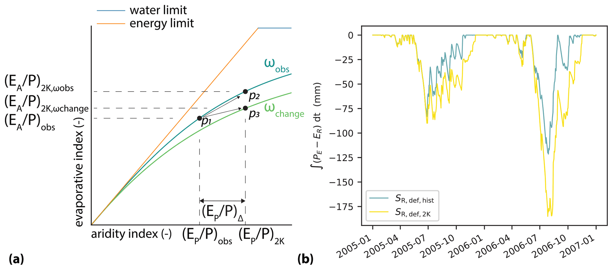
Figure 3 (a) Representation of the Budyko space, which shows the evaporative index ($E_{\mathrm{A}}/P=\mathrm{1}-Q/P$) as a function of the aridity index ($E_{\mathrm{P}}/P$) and the water and energy limit. A catchment with the aridity index $(E_{\mathrm{P}}/P{)}_{\text{obs}}$ and evaporative index $(E_{\mathrm{A}}/P{)}_{\text{obs}}$, which is derived from observed historical data assuming $(E_{\mathrm{A}}/P{)}_{\text{obs}}=\mathrm{1}-(Q/P{)}_{\text{obs}}$, plots at location p₁ on the parametric Budyko curve with ω_obs. A movement in the Budyko space towards p₂ along the ω_obs curve is shown as a result of a change in the aridity index $(E_{\mathrm{P}}/P{)}_{\mathrm{\Delta }}$ towards a projected $(E_{\mathrm{A}}/P{)}_{\mathrm{2}\mathrm{K},\mathit{\omega }\text{obs}}$ associated with aridity $(E_{\mathrm{P}}/P{)}_{\mathrm{2}\mathrm{K}}$. An additional shift from the ω_obs curve towards a location p₃ on a ω_change curve is assumed if additional factors (e.g., land use) are projected to change besides the aridity index. Here, the represented downward shift in ω reduces the change in evaporative index to $(E_{\mathrm{A}}/P{)}_{\mathrm{2}\mathrm{K},\mathit{\omega }\text{change}}$. (b) Cumulative storage deficits (S_R,def) derived from effective precipitation (P_E) and transpiration (E_R), using the simulated historical and 2 K climate data, are shown. Estimates of transpiration (E_R) are derived from long-term water balance projections as a result of movements within the Budyko framework in response to climate and potential land use changes.

4.1 Changing climate, vegetation and land use

4.1.1 Estimating future runoff coefficients

The long-term partitioning of precipitation (P) into evaporation (E_A) and streamflow (Q) is mainly controlled by the long-term aridity index (ratio of potential evaporation over precipitation; $E_{\mathrm{P}}/P$), according to the Budyko hypothesis. To account for additional factors that influence the relation between aridity and the evaporative index $E_{\mathrm{A}}/P$ (and runoff coefficient $Q/P=\mathrm{1}-E_{\mathrm{A}}/P$), Fu (1981) introduces a parameter ω to encapsulate the combined influences of climate, soils, vegetation and topography (Eq. 1). It should be noted that, throughout this paper, we use the term evaporation to represent all different evaporative fluxes (interception, soil evaporation and transpiration), following the terminology proposed by Savenije (2004) and Miralles et al. (2020).

$$\begin{array}{}\text{(1)}& {\displaystyle \frac{E_{\mathrm{A}}}{P}}=\mathrm{1}-{\displaystyle \frac{Q}{P}}=\mathrm{1}+{\displaystyle \frac{E_{\mathrm{P}}}{P}}-(\mathrm{1}+({\displaystyle \frac{E_{\mathrm{P}}}{P}}{)}^{\mathit{\omega }}{)}^{\mathrm{1}/\mathit{\omega }}.\end{array}$$

We solve Eq. (1) to determine the value of ω for each of the 35 catchments of the Meuse basin for observed historical conditions for the period 2005 to 2017 (ω_obs), using the meteorological E-OBS data (P_obs and E_P,obs) and observed streamflow (Q_obs). Assuming only a change in long-term mean climate conditions, i.e., aridity index, a catchment will move along its ω_obs parameterized curve from its original position p₁ to a new position p₂ due to the horizontal shift in aridity index $(E_{\mathrm{P}}/P{)}_{\mathrm{\Delta }}$ (Fig. 3a). Here, we use the simulated historical and 2 K precipitation and potential evaporation climate data to determine how the change in potential evaporation ($\mathrm{\Delta }{E}_{\mathrm{P}}=E_{\mathrm{P},\mathrm{2}\mathrm{K}}-E_{\mathrm{P},\text{hist}}$) and precipitation ($\mathrm{\Delta }P=P_{\mathrm{2}\mathrm{K}}-P_{\text{hist}}$) lead to a change in the aridity index (Eq. 2) and, therefore, in the actual evaporation ($\mathrm{\Delta }{E}_{\mathrm{A}}=E_{\mathrm{A},\mathrm{2}\mathrm{K}}-E_{\mathrm{A},\text{hist}}$) and streamflow ($\mathrm{\Delta }Q=Q_{\mathrm{2}\mathrm{K}}-Q_{\text{obs}}$), using the Budyko hypothesis in Eq. (1).

$$\begin{array}{}\text{(2)}& ({\displaystyle \frac{E_{\mathrm{P}}}{P}}{)}_{\mathrm{2}\mathrm{K}}={\displaystyle \frac{E_{\mathrm{P},\text{obs}}+\mathrm{\Delta }{E}_{\mathrm{P}}}{P_{\text{obs}}+\mathrm{\Delta }P}}.\end{array}$$

However, land cover and vegetation are likely to also change in response to a changing climate, introducing an additional shift toward a position p₃ on a different curve with ω_change (Fig. 3a). A downward shift from ω_obs to ω_change indicates less water use for evaporation, as opposed to an upward shift for higher evaporative water use. These shifts in ω values represent changes in drivers other than the aridity index, including, e.g., land cover, tree species, forest age, biomass growth and water use efficiency (Jaramillo et al., 2018).

To test the sensitivity of the hydrological response to a change in ω in addition to a change in aridity index, we consider two scenarios. The catchments with relatively high percentages of broadleaved forests (25 %–38 %, as in the French part of the basin) receive the ω values of catchments with relatively low percentages of broadleaved forests (1 %–12 %, as mainly in the Belgian Ardennes) and vice versa (Fig. 1b). We denote ω_broadleaved for the catchments with relatively high percentages of broadleaved forests and ω_coniferous for the catchments with relatively low percentages of broadleaved forest, i.e., where broadleaved forests were largely converted to coniferous plantations or agriculture. These scenarios are meant as a sensitivity analysis in the spirit of trading space for time (Singh et al., 2011) to evaluate the effect of potential future land use management on the overall water balance.

When converting broadleaved forest to coniferous plantations, we expect an increase in water use for evaporation and, therefore, an upward shift in ω values, as opposed to a downward shift when converting coniferous plantations to more natural broadleaved forests (Fenicia et al., 2009; Teuling et al., 2019; Stephens et al., 2021). The described movements in the Budyko space are used to estimate the projected long-term runoff coefficients ($(Q/P{)}_{\mathrm{2}\mathrm{K}}$; Eq. 3) as a result of both climate change without changes in vegetation cover (ω_obs) and climate change in combination with changes in vegetation cover (by swapping ω_broadleaved values to ω_coniferous for a selection of catchments and vice versa). The projected runoff coefficients are subsequently used to estimate the long-term projected 2 K evaporation E_A by closing the water balance, which, in turn, allows us to estimate projected transpiration E_R and changes in the root zone storage capacity parameter, as described in detail in Sect. 4.1.2.

$$\begin{array}{}\text{(3)}& \begin{array}{rl}({\displaystyle \frac{Q}{P}}{)}_{\mathrm{2}\mathrm{K},\mathit{\omega }}& ={\displaystyle \frac{Q_{\text{obs}}+\mathrm{\Delta }Q}{P_{\text{obs}}+\mathrm{\Delta }P}}=-\left(\right({\displaystyle \frac{E_{\mathrm{P}}}{P}}{)}_{\mathrm{2}\mathrm{K}}\\ & -(\mathrm{1}+({\displaystyle \frac{E_{\mathrm{P}}}{P}}{)}_{\mathrm{2}\mathrm{K}}^{\mathit{\omega }}{)}^{\mathrm{1}/\mathit{\omega }})=\mathrm{1}-({\displaystyle \frac{E_{\mathrm{A}}}{P}}{)}_{\mathrm{2}\mathrm{K},\mathit{\omega }}.\end{array}\end{array}$$

4.1.2 Estimating the root zone storage capacity $S_{\mathrm{R},max}$

The root zone storage capacity represents the maximum volume of water which can be held against gravity in pores of unsaturated soil and which is accessible to roots of vegetation for transpiration. It is a key element controlling the hydrological response of hydrological systems. The long-term partitioning of precipitation into streamflow and evaporation of catchments worldwide plots closely around the Budyko curve, suggesting that vegetation has adapted its root zone storage capacity to offset hydro-climatic seasonality by creating a buffer large enough to overcome dry spells (Gentine et al., 2012; Donohue et al., 2012; Gao et al., 2014). This is the main assumption underlying the water balance method to estimate the root zone storage capacity at the catchment scale (Gao et al., 2014; Nijzink et al., 2016a; de Boer-Euser et al., 2016; Wang-Erlandsson et al., 2016; Bouaziz et al., 2020; Hrachowitz et al., 2021).

The water balance method requires daily time series of precipitation, potential evaporation and a long-term runoff coefficient to estimate transpiration which depletes the root zone storage during seasonal dry periods. Annual water deficits (S_R,def) stored in the root zone of vegetation to fulfill canopy water demand for transpiration are estimated on a daily time step as the cumulative sum of daily effective precipitation (P_E) minus transpiration (E_R).

First, effective precipitation, i.e., the amount of precipitation that reaches the soil after interception evaporation (E_I), is estimated by solving the water balance of a canopy storage (S_I) with maximum interception storage capacity (I_max; here taken as 2.0 mm), according to (Eq. 4). A value of 2.0 mm for I_max was previously also used by de Boer-Euser et al. (2016) and Bouaziz et al. (2020), who also show a low sensitivity of the root zone storage capacity to the value of I_max.

$$\begin{array}{}\text{(4)}& P_{\mathrm{E}}\left(t\right)=P\left(t\right)-E_{\mathrm{I}}\left(t\right)-{\displaystyle \frac{\mathrm{d}{S}_{\mathrm{I}}\left(t\right)}{\mathrm{d}t}},\end{array}$$

with daily interception evaporation $E_{\mathrm{I}}\left(t\right)=min\left(E_{\mathrm{P}}\right(t),S_{\mathrm{I}}(t)/\mathrm{d}t)$ and daily effective precipitation $P_{\mathrm{E}}\left(t\right)=max(\mathrm{0},(S_{\mathrm{I}}\left(t\right)-I_{max})/\mathrm{d}t)$, both in millimeters per day (mm d⁻¹).

Next, the long-term historical and projected future transpiration ${\stackrel{\mathrm{‾}}{E}}_{\mathrm{R}}$ is estimated from the long-term water balance, using mean annual historical and projected future streamflow, estimated by movements in the Budyko space, and effective precipitation ($\stackrel{\mathrm{‾}}{Q}$ and ${\stackrel{\mathrm{‾}}{P}}_{\mathrm{E}}$, all in millimeters per year (mm yr⁻¹); Eq. 5), assuming negligible changes in storage and inter-catchment groundwater flows (catchments where ${\stackrel{\mathrm{‾}}{E}}_{\mathrm{A}}={\stackrel{\mathrm{‾}}{E}}_{\mathrm{I}}+{\stackrel{\mathrm{‾}}{E}}_{\mathrm{R}}=\stackrel{\mathrm{‾}}{P}-\stackrel{\mathrm{‾}}{Q}<{\stackrel{\mathrm{‾}}{E}}_{\mathrm{P}}$).

$$\begin{array}{}\text{(5)}& {\stackrel{\mathrm{‾}}{E}}_{\mathrm{R}}\approx {\stackrel{\mathrm{‾}}{P}}_{\mathrm{E}}-\stackrel{\mathrm{‾}}{Q}.\end{array}$$

The long-term transpiration ${\stackrel{\mathrm{‾}}{E}}_{\mathrm{R}}$ is subsequently scaled to daily transpiration estimates E_R, using the daily signal of potential evaporation minus interception evaporation, according to Eq. (6) (Nijzink et al., 2016a; Bouaziz et al., 2020).

$$\begin{array}{}\text{(6)}& E_{\mathrm{R}}\left(t\right)=\left(E_{\mathrm{P}}\right(t)-E_{\mathrm{I}}(t\left)\right)\cdot {\displaystyle \frac{{\stackrel{\mathrm{‾}}{E}}_{\mathrm{R}}}{({\stackrel{\mathrm{‾}}{E}}_{\mathrm{P}}-{\stackrel{\mathrm{‾}}{E}}_{\mathrm{I}})}}.\end{array}$$

The maximum annual storage deficits can then be derived from the cumulative difference of effective precipitation (P_E) and transpiration (E_R), assuming an infinite storage, according to Eq. (7) and illustrated in Fig. 3b. For each year, S_R,def represents the amount of water accessible to the roots of vegetation for transpiration during a dry period. Storage deficits are assumed to be zero at the end of the wet period (T₀; here April) and increase when transpiration exceeds effective precipitation during dry periods, until they become zero again (T₁) in the fall and winter when excess precipitation is assumed to drain away as direct runoff or recharge.

$$\begin{array}{}\text{(7)}& S_{\mathrm{R},\text{def}}\left(t\right)=min\underset{T_{\mathrm{0}}}{\overset{T_{\mathrm{1}}}{\int }}\left(P_{\mathrm{E}}\right(t)-E_{\mathrm{R}}(t\left)\right)\mathrm{d}t.\end{array}$$

By fitting the extreme value distribution of Gumbel to the series of annual maximum storage deficits, the root zone storage capacity at the catchment scale $S_{\mathrm{R},max}$ can be derived for various return periods. The Gumbel distribution was previously shown to be a suitable choice for the estimation of the root zone storage capacity through the water balance approach by several other studies (Gao et al., 2014; Nijzink et al., 2016a; de Boer-Euser et al., 2016; Bouaziz et al., 2020; Hrachowitz et al., 2021). These studies used a return period of 20 years for forested areas, suggesting that forests develop root systems to survive droughts with a return period of ∼ 20 years. The root zone storage capacity of cropland and grasslands is assumed to correspond to deficits with lower return periods of ∼ 2 years (Wang-Erlandsson et al., 2016). It should be noted that the methodology assumes that vegetation taps its water from the unsaturated zone and not from groundwater.

Using the above-described methodology, we determine several sets of $S_{\mathrm{R},max}$ values for each of the 35 catchments of the Meuse basin to represent the historical and adapted root zone storage capacity in response to a changing climate and changing/historical land use, using historical climate observations (E-OBS) and the historical and 2 K climate simulations. The estimated adaptation of the root zone storage capacity mainly relates to changes in the rooting system, i.e., rooting density and/or rooting depth. Technical details for the calculation of the various $S_{\mathrm{R},max}$ are given in Sect. S2 in the Supplement.

• $S_{\mathrm{R},max,\mathrm{A}}$ – historical root zone storage capacity. The first set is $S_{\mathrm{R},max,\mathrm{A}}$, which represents the historical meteorological and land use conditions derived from observed historical E-OBS data and observed streamflow data (P_obs, E_P,obs and Q_obs for the period 2005–2017). $S_{\mathrm{R},max,\mathrm{A}}$ is used as parameter for three model runs which are each forced with a different dataset, i.e., historical E-OBS observations, simulated historical and 2 K climate data (Sect. 4.4).

• $S_{\mathrm{R},max,\mathrm{B}}$ – adapted root zone storage capacity in response to a changing climate. We then estimate the root zone storage capacity $S_{\mathrm{R},max,\mathrm{B}}$ based on the 2 K climate and historical land use to reflect the adaptation of existing vegetation to changing climatic conditions such as differences in seasonality, the aridity index (Eq. 2) and the resulting runoff coefficient (Eq. 3) but under the assumption that the vegetation cover remains unchanged (ω_obs).

• $S_{\mathrm{R},max,\mathrm{C}}$ and $S_{\mathrm{R},max,\mathrm{D}}$ – adapted root zone storage capacity in response to a changing climate and land use. Subsequently, the root zone storage capacity is estimated for the 2 K climate under two land use change scenarios, considering that, if climate changes, a different vegetation cover might become dominant under natural and anthropogenic influence. In the first scenario, land use in the catchments with mainly coniferous plantations and agriculture (as mainly seen in the Belgian Ardennes; Sect. 2.2 and Fig. 1) is assumed to be converted to broadleaved forest, while, in the second scenario, the broadleaved forests in the French part of the basin are converted to coniferous plantations and agriculture. To simulate these land use changes, we first group the ω_obs parameter of the Budyko curves of the 35 catchments in three categories according to their areal fraction of broadleaved forest (Fig. 1b). Then, making use of a space-for-time exchange, we randomly sample from the ω_obs values of one category to represent potential future changes in the other category. In other words, we use the ω_obs values of catchments with a high percentage of broadleaved forest to represent a potential conversion of land use to broadleaved forest in catchments with current-day low percentage of broadleaved forest ($S_{\mathrm{R},max,\mathrm{C}}$) and vice versa ($S_{\mathrm{R},max,\mathrm{D}}$). These exchanged ω values are used to estimate the 2 K runoff coefficient with Eq. (3). We repeat this random sampling seven times, which results in seven parameter realizations for each of $S_{\mathrm{R},max,\mathrm{C}}$ and $S_{\mathrm{R},max,\mathrm{D}}$. The sampling is performed because the variability in the ω_obs values in each category is also influenced by other factors besides the dominant presence of broadleaved forest. In the subsequent analyses, we consider the ensemble of individual realizations to account for this uncertainty.

4.2 Hydrological model

The wflow_FLEX-Topo model (de Boer-Euser, 2017; Schellekens et al., 2020) is a fully distributed process-based model which uses different flexible model structures for a selection of Hydrological Response Units (HRUs), delineated from the topography and the land use, to represent the spatial variability in the hydrological processes. Here, we develop a model with three HRUs for wetlands, hillslopes and plateaus connected through their groundwater storage (model schematization and equations in Sect. S3 in the Supplement; Savenije, 2010; de Boer-Euser, 2017). Thresholds of 5.9 m for the height above the nearest drainage (HAND; Rennó et al., 2008) and 0.129 for slope are used to delineate the three HRUs, as suggested by Gharari et al. (2011), using the MERIT (Multi-Error-Removed Improved Terrain) hydro dataset at ∼ 60 m × 90 m resolution (Yamazaki et al., 2019). As an additional step, given the high proportion of forest on the hillslopes and of agriculture on the plateaus, we here associated hillslope with forest and agriculture with plateau, using the CORINE (Coordination of Information on the Environment) land cover data (European Environment Agency, 2018). The areal fraction of each HRU are then derived for each cell at the model resolution of 0.00833^∘ (or ∼ 600 m × 900 m).

The model is forced with precipitation, potential evaporation and temperature. Snow, interception, root zone and fast and slow storage components are included in the model. Actual evaporation from the root zone is linearly reduced when storage is below a certain threshold parameter. This standard formulation to express vegetation water stress (Sect. S3 in the Supplement) is used in many process-based models, including NAM (NedborAfstrommings Model), HBV (Hydrologiska Byråns Vattenbalansavdelning) and VHM (Veralgemeend Conceptueel Hydrologisch Model; Bouaziz et al., 2021). Streamflow is routed through the upscaled river network at the model resolution (Eilander et al., 2021) with the kinematic wave approach. Similar implementations of that model were previously successfully used in a wide variety of environments (e.g., Gharari et al., 2013; Gao et al., 2014; Nijzink et al., 2016b; de Boer-Euser, 2017; Hulsman et al., 2021; Bouaziz et al., 2021).

4.3 Model calibration and evaluation

4.3.1 Calibration and evaluation using the observed historical E-OBS climate data

The wflow_FLEX-Topo model is calibrated using streamflow at Borgharen and the observed historical E-OBS meteorological forcing data for the period 2007–2011, using 2005–2006 as warm-up years. The observed historical E-OBS dataset is used to calibrate the model as it is assumed to most closely represent current-day conditions. The parameter space is explored with a Monte Carlo strategy, sampling 10 000 realizations from uniform prior parameter distributions (Sect. S4 in the Supplement). The limited number of samples is due to the high computational resources required to run the distributed model. However, our aim is not to find the optimal parameter set but rather to retain an ensemble of plausible parameter sets based on a multi-objective calibration strategy (Hulsman et al., 2019). To best reflect different aspects of the hydrograph, including high flows, low flows and medium-term partitioning of precipitation into drainage and evaporation, parameter sets are selected based on their ability to simultaneously and adequately represent four objective functions, including the Nash–Sutcliffe efficiencies of streamflow, the logarithm of streamflow and monthly runoff coefficients, as well as the Kling–Gupta efficiency of streamflow. Only parameter sets that exceed a performance threshold of 0.9 for each metric are retained as feasible. The root zone storage capacity parameter $S_{\mathrm{R},max,\mathrm{A}}$ is a fixed parameter for each subcatchment, which is derived from annual maximum storage deficits with a return period of 2 years for the wetland and plateaus HRUs and 20 years for the hillslopes HRU (Sect. 4.1.2). Next, model performance is evaluated in the 2012–2017 post-calibration period using the same performance metrics, a visual inspection of the hydrographs and the mean monthly streamflow regime. The performance metrics are also evaluated for the 34 remaining nested subcatchments.

4.3.2 Evaluation using the simulated historical climate data

The performance of the calibrated model for the ensemble of retained parameter sets is also evaluated when the model is forced with the simulated historical climate data, using $S_{\mathrm{R},max,\mathrm{A}}$ for the root zone storage capacity parameter. This is the reference historical run against which the relative effect of 2 K global warming is evaluated for different scenarios to enable a fair comparison (Fig. 2 and Sect. 4.4). In addition, in Sect. S5 in the Supplement, we evaluate the performance of the calibrated model forced with the simulated historical climate data but with a root zone storage capacity parameter derived directly from this data.

4.4 Hydrological change evaluation

We then force the calibrated wflow_FLEX-Topo model for the ensemble of retained parameter sets with the same 2 K climate forcing data in four scenarios, each using a different root zone storage capacity parameter to represent either stationary or adapted conditions in response to a changing climate and land use (Fig. 2 and Sect. 4.1.2). Using the same climate forcing for each of the 2 K scenarios implies that we do not change potential evaporation as a result of potential land use changes. In addition, the percentages of each HRU in our model structure are not changed for the potential land use change scenarios. This is because the top-down approach to estimating the effect of land use change does not provide the level of detail required to specifically change land use type at the pixel level.

Figure 4 (a) Budyko space with parametric ω_obs curves for each of the 35 catchments of the Meuse basin. The dashed curves represent the median ω_obs curves for each category of areal broadleaved forest percentage. The change in the median aridity index across the catchments of the three categories, from historical to 2 K climate conditions, is shown by the circles and triangles. (b) Parameterized ω_obs values for each of the 35 catchments of the Meuse basin, categorized according to their percentage of broadleaved forest. (c) Range of root zone storage capacities across the 35 catchments of the Meuse basin for the four scenarios. $S_{\mathrm{R},max,\mathrm{A}}$ represents the root zone storage capacity for historical conditions. $S_{\mathrm{R},max,\mathrm{B}}$ represents an adapted root zone storage capacity in response to the 2 K climate but no land use change. In the estimation of $S_{\mathrm{R},max,\mathrm{C}}$, catchments with a low percentage of broadleaved forest (1 %–12 %) receive ω values sampled from catchments with a high percentage of broadleaved forest (25 %–38 %) to represent changes in land use towards a conversion to broadleaved forest. The same, but reversed, approach is applied for the estimation of $S_{\mathrm{R},max,\mathrm{D}}$.

The difference between the modeled historical hydrological response (1980–2018) and the hydrological responses predicted by each of the four model scenarios based on the 2 K climate is evaluated in terms of runoff coefficient, evaporative index, annual statistics (runoff coefficient, evaporative index, mean, maximum, minimum 7 d streamflow and median annual sum of streamflow below the 90th percentile historical streamflow) and monthly patterns of flux and state variables (streamflow, evaporation, root zone storage and groundwater storage) for a hypothetical 38-year period. The four scenarios, which each use $S_{\mathrm{R},max,\mathrm{A}}$ as root zone storage capacity in the historical run, as shown in Fig. 2, are listed below.

• Scenario 2 K_A – stationarity. In scenario 2 K_A, we assume an unchanged land use and that vegetation has not adapted its root zone storage capacity to the aridity and seasonality of the 2 K climate. This scenario implies the stationarity of model parameters by using $S_{\mathrm{R},max,\mathrm{A}}$ in both the historical and 2 K runs, a common assumption of many climate change impact assessment studies (Booij, 2005; de Wit et al., 2007; Prudhomme et al., 2014; Hakala et al., 2019; Brunner et al., 2019; Gao et al., 2020; Rottler et al., 2020; Hanus et al., 2021). This is the benchmark scenario against which we compare the hydrological response, considering non-stationarity of the system, as in the following three scenarios.

• Scenario 2 K_B – non-stationarity of the root zone storage capacity in response to a changing climate. In scenario 2 K_B, we again assume an unchanged land use (ω_obs). However, we assume that vegetation has adapted its root zone storage capacity to the aridity and seasonality of the 2 K climate conditions by selecting $S_{\mathrm{R},max,\mathrm{B}}$ as a parameter for the 2 K model run.

• Scenario 2 K_C – non-stationarity of the root zone storage capacity in response to a changing climate and land use conversion to broadleaved forest. In scenario 2 K_C, we use the root zone storage capacity $S_{\mathrm{R},max,\mathrm{C}}$ to reflect adaptation in response to the changing aridity index and seasonality of the 2 K climate and changes in vegetation cover for the catchments located mainly in the Belgian Ardennes and dominated by coniferous plantation and agriculture to a land use of broadleaved forest as in the French part of the basin.

• Scenario 2 K_D – non-stationarity of the root zone storage capacity in response to a changing climate and land use conversion to coniferous plantation and agriculture. In scenario 2 K_D, the approach of scenario 2 K_C is repeated. However, now the broadleaved forest in the French catchments are assumed to be converted to coniferous plantations or agriculture as in the Belgian Ardennes. The parameter $S_{\mathrm{R},max,\mathrm{D}}$ is used in the model run forced with the 2 K climate.

5 Results

5.1 Adapted root zone storage capacity $S_{\mathrm{R},max}$

5.1.1 Long-term water balance characteristics across catchments

In solving the parametric Budyko curve (Eq. 1) for the 35 catchments of the Meuse basin using historical E-OBS data and observed streamflow (Fig. 4a), we found that ω_obs values tend to be lower, with a median and standard deviation (subsequent values in the next sections represent the same variables) of 2.43 ± 0.48, for catchments with relatively high percentages of broadleaved forests (25 %–38 %, as in the French part of the basin) as compared to catchments with relatively low percentages of broadleaved forests (1 %–12 %, as in the Belgian part of the catchment), with ω_obs values of 3.04 ± 0.54, as shown in Fig. 4b. Higher values of ω for a same aridity index indicate more water use for evaporation, which is likely related to the increased water use of relatively young coniferous plantations and agriculture as opposed to older broadleaved forests (Fenicia et al., 2009; Teuling et al., 2019).

5.1.2 $S_{\mathrm{R},max,\mathrm{A}}$: historical root zone storage capacity

The root zone storage capacity $S_{\mathrm{R},max,\mathrm{A}}$ derived with observed historical E-OBS climate data and observed streamflow is estimated at values of 100 ± 17 and 169 ± 24 mm across all study catchments for 2- and 20-year return periods, respectively (Fig. 4c).

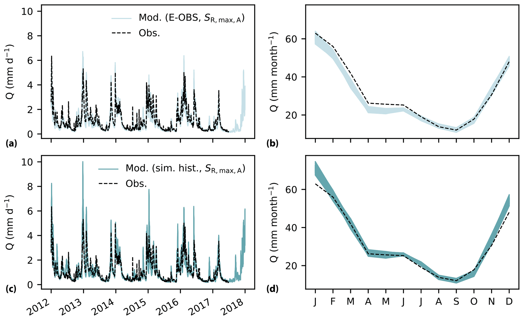
Figure 5 Observed and modeled hydrographs and mean monthly streamflow at Borgharen for the ensemble of parameter sets retained as feasible after calibration when the model is (a, b) forced with E-OBS historical data, using $S_{\mathrm{R},max,\mathrm{A}}$ as the model parameter, and (c, d) forced with the simulated historical climate data, using $S_{\mathrm{R},max,\mathrm{A}}$ as model parameter.

5.1.3 $S_{\mathrm{R},max,\mathrm{B}}$: adapted root zone storage capacity in response to a changing climate

The adapted root zone storage capacity $S_{\mathrm{R},max,\mathrm{B}}$, in response to changing climate conditions and an unchanged land use, strongly increases with respect to historical conditions ($S_{\mathrm{R},max,\mathrm{A}}$) with estimated values of 127 ± 18 mm (+27 %) and 226 ± 27 mm (+34 %) for return periods of 2 and 20 years, respectively (Fig. 4c). This strong increase is explained by larger storage deficits during summer due to an increase of about +10 % in the summer potential evaporation in the 2 K climate and, therefore, a more pronounced seasonality (Fig. 3b). In contrast, the change in the aridity index between the historical and 2 K climate simulations is relatively small with a median of +0.01 across all study catchments. This can be explained by a simultaneous increase in the mean annual precipitation (+4 %) and potential evaporation (+7 %) on average over the basin area in the 2 K climate compared to the simulated historical climate data. This increase in precipitation mostly occurs during the winter half year (November–April). In contrast, there is a relatively large variability in the precipitation change in summer, which is characterized by years with wetter and drier summers.

5.1.4 $S_{\mathrm{R},max,\mathrm{C}}$: adapted root zone storage capacity in response to a changing climate and land use conversion to broadleaved forest

The adapted root zone storage capacity $S_{\mathrm{R},max,\mathrm{C}}$, in response to changing climate conditions and a land use conversion from coniferous plantation and agriculture to broadleaved forest, results in estimated values of 123 ± 17 and 216 ± 27 mm for return periods of 2 and 20 years, respectively (Fig. 4c). These values are similar to $S_{\mathrm{R},max,\mathrm{B}}$, with a difference of about −4 %. This small decrease is in line with the expected reduced water use of broadleaved forests compared to coniferous plantations.

5.1.5 $S_{\mathrm{R},max,\mathrm{D}}$: adapted root zone storage capacity in response to a changing climate and land use conversion to coniferous plantation and agriculture

In contrast, the root zone storage capacity $S_{\mathrm{R},max,\mathrm{D}}$, in response to changing climate conditions and a conversion of broadleaved forest to coniferous plantation, results in estimated values of 137 ± 22 and 235 ± 35 mm for return periods of 2 and 20 years, respectively (Fig. 4c). This corresponds to an additional increase of +8 % and +4 % for both return periods in comparison with $S_{\mathrm{R},max,\mathrm{B}}$, which does not consider additional land use changes.

Therefore, the increase in root zone storage capacity between the 2 K and historical climate simulations can, here by +57 mm or +34 % for a return period of 20 years, be mostly attributed to a changing climate (aridity and seasonality) than to changes in land use (−10 mm or −4 % for $S_{\mathrm{R},max,\mathrm{C}}$ and +9 mm or +4 % for $S_{\mathrm{R},max,\mathrm{D}}$). This indicates that, with the assumed land use change in scenarios 2 K_C and 2 K_D, the strong increase in water demand during summer as a result of a more pronounced seasonality has a greater impact on the estimation of the root zone storage capacity than a change in ω values. However, note that land use is changed only in part of the catchment for both land use change scenarios and that it is plausible to assume that more pronounced changes in land use will reinforce the observed effects.

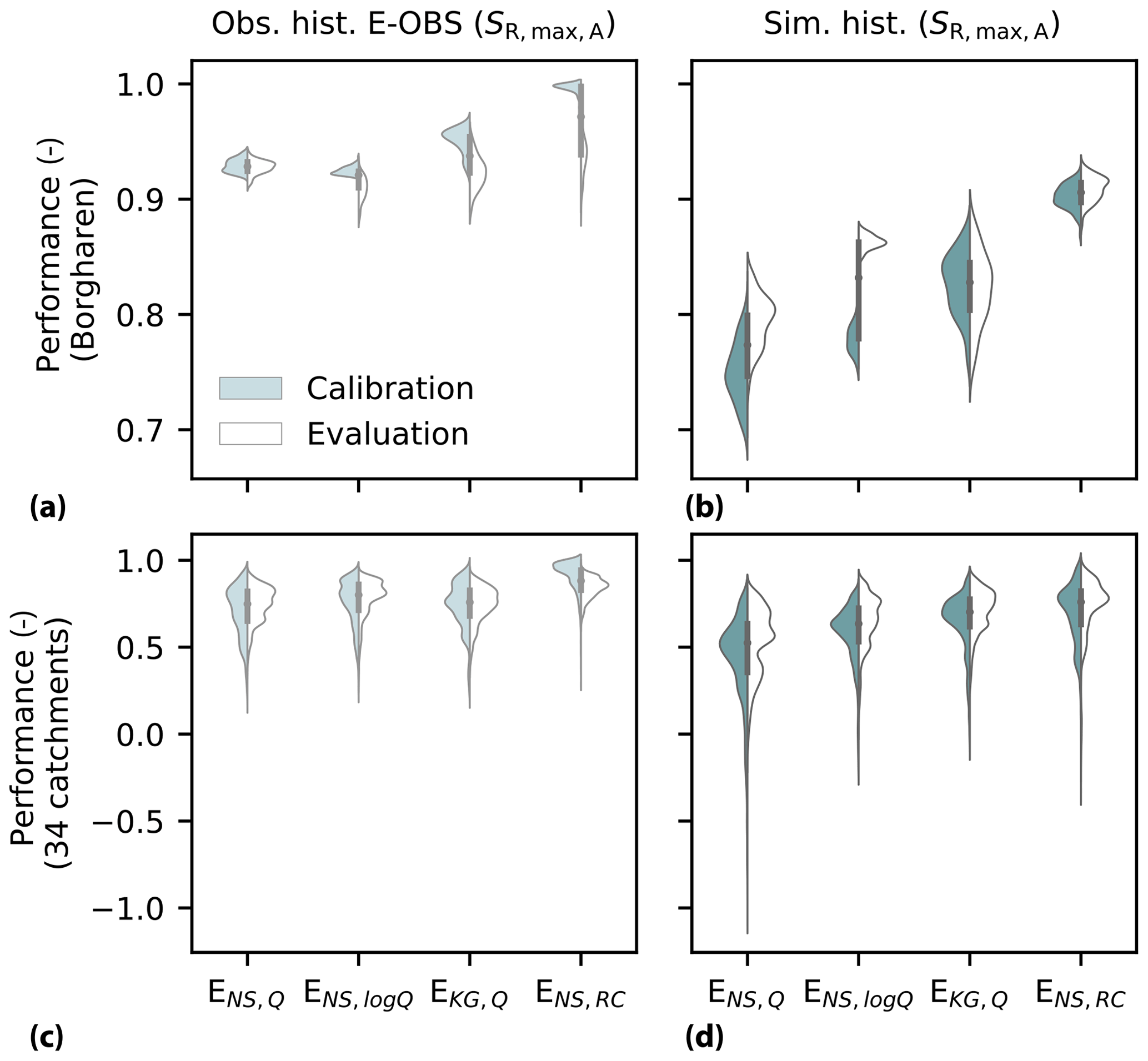
Figure 6 Streamflow model performance during calibration and evaluation for the four objective functions when the model is forced with (a, c) observed historical E-OBS data and (b, d) simulated historical climate data at (a, b) Borgharen and (c, d) for the ensemble of nested catchments in the Meuse basin. The four objective functions are the Nash–Sutcliffe efficiencies of streamflow, logarithm of streamflow and monthly runoff coefficient (E_NS,Q, E_NS,log Q and E_NS,RC), as well as the Kling–Gupta efficiency of streamflow (E_KG,Q). Note the different y-axis scales between rows.

5.2 Model evaluation (historical period)

5.2.1 Model forced with observed historical climate data

The modeled streamflow mimics the observed hydrograph at Borgharen reasonably well for the evaluation period when using the ensemble of parameter sets retained as feasible after calibration (Fig. 5a). Also, the seasonal streamflow regime is well reproduced by the model, except for an underestimation of −9 % in the first half-year (Fig. 5b). The four objective functions show a relatively similar performance during calibration and evaluation, with median values of 0.93 and 0.78 at Borgharen, and for the ensemble of 34 additional, not individually calibrated, nested subcatchments of the Meuse, respectively (Fig. 6a and c).

5.2.2 Model forced with simulated historical climate data

When the calibrated model is instead forced with the simulated historical climate data, peaks are slightly overestimated in comparison to the model run forced with the observed historical E-OBS data (Fig. 5c). This is due to the, on average, +9 % overestimation of precipitation in the simulated historical climate data compared to the observed historical E-OBS climate data. This precipitation overestimation results in an overestimation of about +12 % of the modeled mean monthly streamflow during the wet December and January months (Fig. 5d). However, flows in spring and early summer are better captured when using the simulated historical climate data instead of historical E-OBS data (Fig. 5d). Overall, the streamflow model performance at Borgharen slightly decreases when the simulated historical climate data is used instead of E-OBS, but median values across the ensemble of feasible parameter sets are still above 0.77 for each of the objective functions (Fig. 6b). Although a decrease in model performance is found in a few nested catchments, the performance in the ensemble of nested catchments of the Meuse remains at median values of around 0.67 (Fig. 6d). The results of the model run forced with the simulated historical data and with the root zone storage capacity parameter derived directly from this data show a relatively similar behavior, as further detailed in Sect. S5 in the Supplement.

The calibrated model forced with the simulated historical climate data shows a plausible behavior with respect to observed streamflow and is also reasonably close to the performance achieved with the observed historical E-OBS climate data. This is important because the effect of the 2 K climate on the hydrological response is evaluated with respect to the model run forced with the simulated historical climate data, as they are both generated with the regional climate model. Therefore, the relatively high model performance in the evaluation period enables us to use the retained parameter sets from the calibration with E-OBS data for the subsequent analyses with the simulated historical and 2 K climate data.

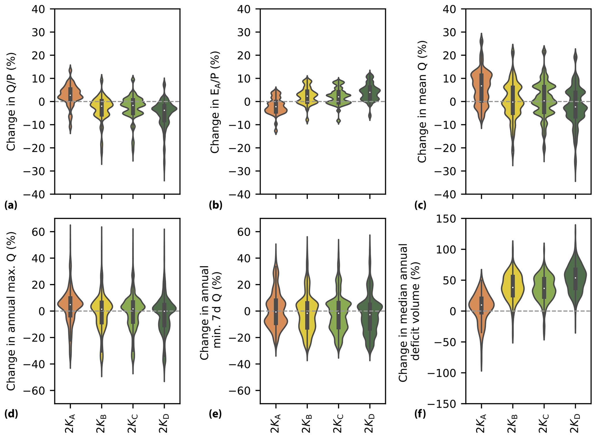
Figure 7 Percentage change in annual hydrological response indicators between the 2 K and historical model runs for the four scenarios, each based on different assumptions for the root zone storage capacity parameter $S_{\mathrm{R},max}$. The percentage change in the (a) runoff coefficient $Q/P$, (b) evaporative index $E_{\mathrm{A}}/P$, (c) mean annual streamflow, (d) mean annual maximum streamflow, (e) minimum annual 7 d mean streamflow and (f) median annual deficit volume below the reference 90th percentile streamflow is shown. Note the different y-axis scales.

5.3 Hydrological change evaluation (2 K warmer climate)

5.3.1 Scenario 2 K_A: stationarity

In the 2 K_A scenario, representing a stationary system with identical parameters in the historical and 2 K climate, runoff coefficients are projected to increase, with a median of +3 %, the evaporative index ($E_{\mathrm{A}}/P$) decreases with a median of −2 % and mean annual streamflow increases with a median of +7 %. Maximum annual streamflow is also projected to increase with a median of about +5 %, while the median change in annual minimum of 7 d mean streamflow remains close to zero. The median annual sum of streamflow below the 90th percentile historical streamflow increases by +10 %, as shown in Fig. 7.

Figure 8 Percentage change in the mean monthly hydrological response of several flux and state variables between 2 K and historical model runs for the four scenarios, each based on different assumptions for the root zone storage capacity parameter $S_{\mathrm{R},max}$. The percentage change in mean monthly (a) streamflow Q, (b) root zone storage S_R, (c) actual evaporation E_A and (d) groundwater storage S_S is shown. The lines and shaded areas show the median and 5th–95th percentiles from the ensemble of parameter sets retained as feasible.

From the intra-annual perspective, streamflow is projected to increase from December until August, by +8 % on average, and decrease between September and November, by −7 % (Fig. 8a). In the months where evaporation demand exceeds precipitation, the root zone soil moisture decreases, with a maximum of −22 % in September (Fig. 8b). Actual evaporation increases throughout the year by around +3 % on average, except in July and August (−4 %), when the availability of water in the root zone of vegetation is not sufficient to supply canopy water demand (Fig. 8c). The groundwater storage increases by approximately +5 % in all months except November, as shown in Fig. 8d.

5.3.2 Scenario 2 K_B: non-stationarity of the root zone storage capacity in response to a changing climate

Changes are substantially different in the 2 K_B scenario, which considers that the root zone storage capacity of vegetation has adapted to the change in the aridity and seasonality of the 2 K climate. In contrast to scenario 2 K_A, runoff coefficients are projected to decrease with a median of −2 %, while the evaporative index increases with a median of +2 % and the median change of mean annual streamflow is close to zero (Fig. 7). Similarly, the median change of both the annual maximum streamflow and minimum 7 d mean streamflow remains close to zero. However, there is a substantial increase of +38 % in the median annual sum of streamflow below the 90th percentile historical streamflow. This result suggests that, while the minimum streamflow remains relatively similar, the length of the low-flow period strongly increases when considering an adaptation of the root zone storage capacity to the 2 K climate (Fig. 7).

Seasonal changes indicate a decrease in streamflow of −19 % between September and November, which is longer and considerably more pronounced than in the 2 K_A scenario (Fig. 8a). The root zone soil moisture increases throughout the year, with an average of +34 %, due to the larger root zone storage capacities (Fig. 8b). Actual evaporation is no longer reduced as a result of moisture stress in the root zone that has adapted to a changing climate and strongly increases by, on average, approximately +7 % from May to October to supply canopy water demand (Fig. 8c). However, the considerable increase in spring and summer evaporation strongly reduces the groundwater storage by −5 % from October to February (Fig. 8d).

5.3.3 Scenario 2 K_C: non-stationarity of the root zone storage capacity in response to a changing climate and land use conversion to broadleaved forest

The predicted hydrological response in the 2 K_C scenario is very similar to the response of the 2 K_B scenario, despite considering additional changes in the root zone storage capacity as a result of a land use conversion from coniferous plantations and agriculture to broadleaved forest (Figs. 7 and 8). This is in line with the limited differences in root zone storage capacities of around only +4 % between both scenarios (Sect. 5.1).

5.3.4 Scenario 2 K_D: non-stationarity of the root zone storage capacity in response to a changing climate and land use conversion to coniferous plantation and agriculture

In contrast, the change in hydrological response is most pronounced for the scenario $S_{\mathrm{R},max,\mathrm{D}}$, which considers the land use conversion of the broadleaved forests in the French part of the basin to coniferous plantations and agriculture (Figs. 7 and 8). Runoff coefficients decrease with a median of −4 %, while the evaporative index increases with a median value of +4 % and mean annual streamflow decreases with a median of −2 %, as opposed to a +5 % increase in the stationary 2 K_A scenario (Fig. 7a–c). While the median change in streamflow extremes remains relatively close to zero, there is a strong increase of +54 % in the median annual sum of streamflow below the 90th percentile historical streamflow, suggesting a strong increase in the length of the low-flow period (Fig. 7d–f).

Streamflow decreases from August to January, with an average of −23 %, and evaporation strongly increases from May to October, with an average of +9 %. This increased evaporation during summer further reduces the groundwater storage from October to February by −7 % (Fig. 8). In comparison with the hydrological response of scenario 2 K_B, the additional land use conversion in scenario 2 K_D results in relatively similar patterns of change but with an additional +2 % increase in evaporation, −2 % decrease in streamflow and −2 % decrease in groundwater storage, on average, throughout the year.

5.3.5 Stationary versus adaptive ecosystems

There is a difference of up to −7 % in the change in mean annual streamflow between the stationary scenario 2 K_A and the scenarios 2 K_B, 2 K_C and 2 K_D with adaptive ecosystems (Fig. 7c). Additionally, the scenarios with adaptive ecosystems show a substantially more pronounced decrease in streamflow from September to January and a delay in the occurrence of the lowest streamflow from September to October (Fig. 8a). Associated to these seasonal differences in streamflow, the scenarios with adaptive ecosystems are characterized by summer evaporation that is up to +14 % higher and a mean annual evaporation that is around +4 % higher than in the stationary scenario (Fig. 8c). Instead of a year-round increase in groundwater storage in the 2 K_A scenario, there is a decrease in winter groundwater storage in the three other scenarios, resulting in a mean annual difference of −6 % between the scenarios with ecosystem adaption and the stationary scenario 2 K_A, expressed as constant model parameters (Fig. 8d). Overall, these results suggest that the hydrological response in the 2 K climate of the stationary scenario 2 K_A is substantially different from the responses of the three scenarios, 2 K_B, 2 K_C and 2 K_D, which consider a change in the root zone storage capacity to reflect ecosystem adaptation in response to climate change.

6 Discussion

6.1 Implications

Current practice in many climate change assessment studies is to assume unchanged system properties in the future (benchmark scenario 2 K_A in our analysis), thereby neglecting potential changes in the system, such as the adaption of vegetation to local climate conditions. In addition to this scenario, we suggest a possible approach to consider ecosystem adaptation in response to climate change and test the sensitivity in the resulting hydrological response. Our analysis is, therefore, a first step in evaluating what may happen if we consider ecosystem adaptation in response to climate change in hydrological model predictions. The hydrological response under 2 K global warming compared to historical conditions shows distinct patterns of change if we explicitly consider the non-stationarity of climate–vegetation interactions in a process-based hydrological model. More specifically, in the non-stationary scenarios, there is an up to −15 % and −10 % additional decrease in streamflow and groundwater storage, respectively, after summer due to an up to +14 % additional increase in actual evaporation during the warmer summers, compared to the stationary scenario. These results suggest a substantially different hydrological response between the stationary and the non-stationary scenarios. However, the additional land use conversion has a relatively limited effect within the non-stationary scenarios, which could be attributed to the limited areal fraction of land use conversion.

Our method is based on readily available data and is, therefore, widely applicable. The choice of hydrological model is open, as root zone storage capacity estimates derived from the water balance approach are applicable in various hydrological and land surface models, provided that they include a root zone parameterization, which is the case for most models (Clark et al., 2008; Nijzink et al., 2016a; Bouaziz et al., 2021; van Oorschot et al., 2021). The water balance approach to estimate the root zone storage capacity has previously been successfully applied in a variety of climate zones and across various ecosystems (Donohue et al., 2012; Gentine et al., 2012; Gao et al., 2014; Wang-Erlandsson et al., 2016; de Boer-Euser et al., 2016; Singh et al., 2020; Hrachowitz et al., 2021; Dralle et al., 2021; McCormick et al., 2021). Here, the estimated values of the root zone storage capacity for the different scenarios have median values below 250 mm for a return period of 20 years, which is within the range of global root zone storage capacity values estimated by Wang-Erlandsson et al. (2016).

A time-dynamic parameterization of the root zone storage capacity in the context of deforestation was previously introduced by Nijzink et al. (2016a) and Hrachowitz et al. (2021), who demonstrated that an observed 20 % increase in the runoff coefficient in a catchment can, to a large extent, be attributed to the > 20 % reduction in root zone storage capacity after deforestation. Speich et al. (2020) implemented a time-dynamic root zone storage capacity in the context of climate change. In their study, forest growth in response to climate change leads to a 6 times higher reduction in streamflow if a dynamic representation of both the leaf area index and the root zone storage capacity is implemented, as opposed to a study in which only the leaf area index varies (Schattan et al., 2013). Although these results are more pronounced than our findings, they point to the same direction of change. As the future is unknown, we cannot test our results against observations, but given the changes in temperature and precipitation, the future predicted hydrological response does not seem implausible. While Speich et al. (2020) combine a forest landscape model with a hydrological model to simultaneously represent the spatiotemporal forest and water balance dynamics, we rely on a simpler approach of movements in the Budyko framework to include potential land use change.

The impact of climate change on low flows in the Meuse basin has been previously studied by de Wit et al. (2007). Using simulations from regional climate models which project wetter winters and drier summers, they question if the increase in winter precipitation reduces the occurrence of summer low flows due to an increase in groundwater recharge. However, they were unable to address this question with their model due to its poor low-flow performance. Our results indicate an increase in groundwater storage during winter in the stationary scenario, as opposed to a decrease for the models with a time-dynamic root zone storage capacity, as a result of an increased water demand for evaporation during summer. In comparing several scenarios for the root zone storage capacity parameter, we include some form of system representation uncertainty, which improves our understanding in the modeled changes by placing them in a broader context (Blöschl and Montanari, 2010). Despite considerable uncertainty regarding the capacity of vegetation to adapt (Sect. 6.2.1), we quantify, with the best of our knowledge, an envelope of the hydrological response by considering the potential degree of ecosystem adaptation to climate change.

The conversion to native species may increase biodiversity and the resilience of ecosystems to climate change (Schelhaas et al., 2003; Klingen, 2017; Levia et al., 2020). However, these processes are slow, implying that current management practices shape the forests of decades and centuries to come in an uncertain future. Increasing our understanding of how to include vegetation changes in hydrological models to reliably quantify their impact is a way forward in the development of strategies to mitigate the adverse effects of climate change.

6.2 Limitations and knowledge gaps

6.2.1 On the estimation of adapted root zone storage capacities

The proposed methodology to estimate future root zone storage capacities relies on the underlying assumption that past empirical relations between aridity index and evaporative index (i.e., the Budyko framework) still apply in the future. While the Budyko framework is a well-established concept, recent studies by Berghuijs et al. (2020) and Reaver et al. (2020) show that it should be cautiously applied in changing systems. The Budyko framework reflects the long-term hydrological partitioning under dynamic equilibrium conditions. Therefore, when using the Budyko framework to estimate the future rate of transpiration, we assume that the future vegetation has adapted to the future climatic conditions and that it is in a state of dynamic equilibrium. The uncertainty of this assumption is considerable because it implies that vegetation has had the time to adapt to the rapidly changing environmental conditions. There is increasing evidence that vegetation will eventually adapt to ensure sufficient access to water (Guswa, 2008; Schymanski et al., 2008; Gentine et al., 2012); otherwise, we would not see the hydrological partitioning of catchments around the world broadly plotting along the Budyko curve (Troch et al., 2013). Yet, considering the unprecedented scale and rate of change (Gleeson et al., 2020), it is unclear how ecosystems will cope with climate change, also considering the impact of potentially increasing storm intensities and frequencies, heat waves, fires and biotic infestations as a result of water stress on forest ecosystems (Lebourgeois and Mérian, 2011; Allen et al., 2010; Latte et al., 2017; Stephens et al., 2021). In particular, there is considerable uncertainty on how long it will take for vegetation to adapt and how it will adapt, assuming thresholds of adaptability are not exceeded.

In this analysis, we did not explicitly consider that vegetation can adapt to drier conditions by regulating its stomata and, hence, reduce transpiration. Furthermore, there is evidence that increasing atmospheric CO₂ concentrations may increase both water use efficiency and also increase green foliage due to fertilization effects (Keenan et al., 2013; Donohue et al., 2013; van der Velde et al., 2014; Frank et al., 2015; van Der Sleen et al., 2015; Ukkola et al., 2016; Jaramillo et al., 2018; Yang et al., 2019; Stephens et al., 2020). While the adaptation strategies of individual plants, e.g., root biomass adjustments, anatomical alterations and physiological acclimatization, depend on vegetation type and species (Brunner et al., 2015; Zhang et al., 2020), here, we determine effective values of the root zone storage capacity at the catchment scale to reflect the adaptation of the whole ecosystem. Yet, our ability to predict what will happen is limited, but we can at least test the sensitivity of the hydrological response to changes in the system representation.

Once future transpiration rates are estimated, the water balance approach to estimate the root zone storage capacity is also subject to limitations. The method is not suitable in areas where the water table is very close to the surface and where vegetation directly can tap from the available groundwater instead of creating a buffer capacity (e.g Fan et al., 2017). Another limitation of the water balance approach relates to Eq. (6), in which we scale the daily transpiration estimates with a constant factor to the patterns of potential evaporation minus interception evaporation, implying that vegetation can extract water for transpiration from dry soils as easily as from wet soils.

6.2.2 On the potential land use change scenarios

We quantify the changes in the hydrological response as a result of a changing climate in combination with several land use scenarios (historical, conversion of broadleaved forests to coniferous plantations and agriculture and vice versa). The relatively limited additional effects of land use change on the hydrological response should be understood in the context of the relatively limited areal fraction under potential land use conversion.

The land use changes are integrated in the root zone storage capacity as a single parameter. However, climate and land use changes likely affect other aspects of catchment functioning, e.g., interception, infiltration and runoff generation (Seibert and van Meerveld, 2016). Changes in the maximum interception storage capacity (Calder et al., 2003) are not explicitly considered in the estimation of the adapted root zone storage capacities in the land use change scenarios, as the impact was shown to be relatively minor in Bouaziz et al. (2020). Additional effects of soil compaction and artificial drainage on peak flows as a result of potential future land conversion (Buytaert and Beven, 2009; Seibert and van Meerveld, 2016) are difficult to quantify but may partly be captured in the changed ω values. As mutual interactions between parameters remain problematic to quantify, we use an ensemble of parameter sets to somehow account for the uncertainty in model parameters and the possibility that parameters compensate for each other due to simplistic process representation.

While ω values are likely a manifestation of multiple climatic, landscape and vegetation characteristics, and may change due to climatic variability, CO₂ vegetation feedbacks and/or anthropogenic modifications (Berghuijs et al., 2017), we assumed that vegetation type is the dominant control to explain differences in ω values. As this parameter describes the hydrological partitioning, and because transpiration is a major continental flux (Jasechko, 2018; Teuling et al., 2019), it is reasonable to assume that the variability in ω values is largely controlled by the water volume accessible to the roots of vegetation for transpiration (i.e., $S_{\mathrm{R},max}$). This root-accessible water volume is independent from the soil type, as root systems will develop in a way to ensure sufficient access to water (Kleidon and Heimann, 1998; Guswa, 2008). In clayey soils, the rooting depth might be shallower than in sandy soils for an identical root zone storage capacity (de Boer-Euser et al., 2016). Topography, geology and soil type are likely implicitly integrated in other model parameters, e.g., the various recession timescales of the linear reservoirs, which represent subsurface flow resistance throughout the system.

We also did not consider how the relatively high ω values may be related to inter-catchment groundwater losses (Bouaziz et al., 2018). Note that, as our analyses should be understood in the context of a sensitivity analysis of the impact of potential additional vertical shifts in the Budyko space as a result of a changing land use (Fig. 3), the potential effects of groundwater losses on the results are likely to be minor.

6.2.3 On the calibration

Last, we performed a limited calibration of the hydrological model to retain an ensemble of plausible solutions and only used a single climate simulation despite the uncertainty in initial and boundary conditions of regional climate models. Our analyses are intended as a sensitivity analysis to quantify the effect of the non-stationarity of the root zone storage capacity parameter on hydrological model predictions, through the optimal use of projected climate data, rather than a comprehensive climate change impact assessment of the Meuse basin.

6.3 Outlook

6.3.1 Applications in land surface and ecohydrological models

The land surface scheme HTESSEL that is used in the regional climate model RACMO2 to generate the historical and 2 K climate simulations assumes, as most land surface models do, a fixed root zone storage capacity over time. Ideally, this discrepancy between the land surface model and the non-stationary hydrological models could be reduced by updating the adapted root zone storage capacity from one model to the other in several iteration steps, thereby including soil moisture–atmosphere feedback mechanisms. The implementation of the root zone storage capacity parameter estimated from water balance data in land surface models is, however, not trivial and requires further research (van Oorschot et al., 2021). Accounting for this climate control on root development and root zone parameterization in ecohydrological models could potentially improve the estimation of evaporative fluxes (Stevens et al., 2020; van Oorschot et al., 2021), as rooting depth and root distributions estimates are often estimated from fixed look-up tables (Tietjen et al., 2017; Schaphoff et al., 2018).

6.3.2 Climate analogues or trading space for time

The concept of trading space for time, which uses space as a proxy for time (Singh et al., 2011), could be further explored by selecting regions outside the Meuse basin with a current climate similar to the projected climate. This approach is also commonly referred to as climate analogue mapping, i.e., statistical techniques to quantify the similarity between the future climate of a given location and the current climate of another location (Rohat et al., 2018; Bastin et al., 2019; Fitzpatrick and Dunn, 2019). This climate matching could be applied over distant regions, using datasets which combine landscape and climatological data over large samples of catchments (e.g., the various Catchment Attributes and Meteorology for Large-sample Studies (CAMELS) datasets; Addor et al., 2017; Klingler et al., 2021). Despite considerable uncertainties, finding a climate analogue for future projections in present conditions may allow us to estimate future ω or root zone storage capacity values in a region where the future climate may resemble today's climate elsewhere. This data-driven approach could potentially lead to more robust estimates of future ω or root zone storage capacity values in response to changes in various climate or landscape indicators. These methods are intuitive but not straightforward, as they rely on the selection and combination of relevant climate variables and their relation with vegetation, despite nonlinear vegetation responses to climate change (Reu et al., 2014).

7 Conclusions

Understanding the non-stationarity of hydrological systems under climate and environmental changes has been recognized as a major challenge in hydrology (Blöschl et al., 2019). Despite our strong awareness of the non-stationarity of hydrological parameters, we often lack knowledge to implement system changes in hydrological models. In this study in the Meuse basin, we introduce a method to estimate future changes in vegetation model parameters, and we evaluate the sensitivity of hydrological model predictions to these changes in vegetation parameters as a result of ecosystem adaptation in response to climate and land use changes. Our top-down approach uses readily available regional climate model simulations to allow a time-dynamic representation of the root zone storage capacity, which is a key parameter in process-based hydrological models. Our approach relies, on the one hand, on a space-for-time exchange of Budyko characteristics of dominant land use types to estimate the hydrological behavior of potential land use changes and, on the other hand, on the interplay between the long-term and seasonal water budgets to represent climate–vegetation interactions under climate and land use change. Despite knowledge gaps regarding future ecosystem water use, we implement potential system changes in a hydrological model based on our current understanding of hydrological systems. The predicted hydrological response to 2 K warming is strongly altered if we consider that vegetation has adapted by increasing its root zone storage capacity by 34 % to offset the more pronounced hydro-climatic seasonality under 2 K global warming compared to a stationary system. The increased vegetation water demand under global warming results annually, and on average, in −7 % less streamflow, +4 % more evaporation and −6 % less groundwater storage for the scenarios assuming non-stationary conditions compared to a stationary system. These differences even imply decreasing instead of increasing median annual streamflow under 2 K global warming under non-stationary conditions. More importantly, the seasonal changes are considerable, with up to +14 % higher evaporation in summer and up to −15 % and −10 % lower streamflow and groundwater storage, respectively, in autumn for the non-stationary scenarios. Our study contributes to the quest for more plausible representations of catchment properties under change and, therefore, more reliable long-term hydrological predictions.