the Creative Commons Attribution 4.0 License.
the Creative Commons Attribution 4.0 License.
 | 12 Jan 2022
Parsimonious statistical learning models for low-flow estimation
Johannes Laimighofer
Michael Melcher
Gregor Laaha
Statistical learning methods offer a promising approach for low-flow regionalization. We examine seven statistical learning models (Lasso, linear, and nonlinear-model-based boosting, sparse partial least squares, principal component regression, random forest, and support vector regression) for the prediction of winter and summer low flow based on a hydrologically diverse dataset of 260 catchments in Austria. In order to produce sparse models, we adapt the recursive feature elimination for variable preselection and propose using three different variable ranking methods (conditional forest, Lasso, and linear model-based boosting) for each of the prediction models. Results are evaluated for the low-flow characteristic Q95 standardized by catchment area using a repeated nested cross-validation scheme. We found a generally high prediction accuracy for winter ( of 0.66 to 0.7) and summer ( of 0.83 to 0.86). The models perform similarly to or slightly better than a top-kriging model that constitutes the current benchmark for the study area. The best-performing models are support vector regression (winter) and nonlinear model-based boosting (summer), but linear models exhibit similar prediction accuracy. The use of variable preselection can significantly reduce the complexity of all the models with only a small loss of performance. The so-obtained learning models are more parsimonious and thus easier to interpret and more robust when predicting at ungauged sites. A direct comparison of linear and nonlinear models reveals that nonlinear processes can be sufficiently captured by linear learning models, so there is no need to use more complex models or to add nonlinear effects. When performing low-flow regionalization in a seasonal climate, the temporal stratification into summer and winter low flows was shown to increase the predictive performance of all learning models, offering an alternative to catchment grouping that is recommended otherwise.
- Article
(2674 KB) - Full-text XML
- BibTeX
- EndNote


Estimating long-term averages of low flow in ungauged basins is crucial for a wide range of applications, e.g., water resource management and engineering, hydropower planning, or ecological issues (Smakhtin, 2001). The two main approaches for predicting low-flow indices are based on either physically based models (e.g., Euser et al., 2013) or statistical models. Statistical low-flow models can be further subdivided into geostatistical models (e.g., Castiglioni et al., 2009, 2011; Laaha et al., 2014) and regression-based methods (e.g., Laaha and Blöschl, 2006, 2007); an overview is given by Salinas et al. (2013). Regression methods cover a wide spectrum of models, and especially in the last decade there was increasing interest in statistical learning models in hydrology (Abrahart et al., 2012; Dawson and Wilby, 2001; Nearing et al., 2021; Solomatine and Ostfeld, 2008), with the terms “statistical learning” and “machine learning” being used synonymously. The applications include rainfall–runoff modeling by neural networks (e.g., Kratzert et al., 2019a, b), using support vector machines (SVM) for prediction of karst tracers (Mewes et al., 2020) or reference evapotranspiration (Tabari et al., 2012) and random forest for flood event classification (Oppel and Mewes, 2020). Nevertheless, the implementation of statistical learning methods for predicting low flow is still rare.
The considered methods so far can be classified as linear and nonlinear statistical learners. Linear methods also include, besides ordinary least squares regression approaches (OLS, Kroll and Song, 2013; Zhang et al., 2018; Ferreira et al., 2021), linear models with a penalization parameter like elastic net (Worland et al., 2018) and linear boosting models (Tyralis et al., 2021). Further approaches are based on dimension reduction techniques such as partial least squares regression (PLS, Kroll and Song, 2013) or principal component regression (PCR, Kroll and Song, 2013; Nosrati et al., 2015). An example of nonlinear extensions to the linear model is the enhanced adaptive regression through hinges (Earth, Ferreira et al., 2021). Furthermore, various forms of tree-based methods were applied in low-flow prediction, such as random forest (RF, Ferreira et al., 2021; Zhang et al., 2018; Worland et al., 2018), gradient boosting with tree stumps (Tyralis et al., 2021) or M5-cubist (Worland et al., 2018). Additionally, the most comparative study of Worland et al. (2018) used an ensemble learning technique called meta M5-cubist, a nonlinear kernel extension of K-nearest neighbor (KKNN) and two variants of support vector regression (polynomial and Gaussian kernel).
Given the large number of learning methods, it is a priori unclear which method will perform best for a particular study area. Only a few studies have conducted a comparative assessment, typically focusing on single methods or a particular group of learners (Kroll and Song, 2013; Zhang et al., 2018; Worland et al., 2018; Ferreira et al., 2021). Comparing only linear models (PLS, PCR, OLS), Kroll and Song (2012) could not find any superior model for 130 stations in the eastern USA. Tree-based methods performed better in terms of point prediction for the CAMELS dataset (Tyralis et al., 2021) or an Australian dataset of 605 stations (Zhang et al., 2018), but both studies showed good performance of less complex linear models. Ferreira et al. (2021) showed that Earth and RF perform similarly for 51 stations in Brazil, and Worland et al. (2018) achieved good performance in terms of a root mean squared error (RMSE) for the ensemble learning model analyzing 224 stations in the southeastern USA. All of these studies were conducted for different hydroclimatic settings, but none did focus on a seasonal climate, where low flows in summer and winter are generated by different processes and should be assessed separately. Such an assessment is missing and will be addressed in this study.
Results of Worland et al. (2018) and Ferreira et al. (2021) indicate that more complex models seem to perform better than more parsimonious ones, making model interpretation difficult and plausibility of parameters hard to judge. This leads to a major criticism of statistical learning models, as they are often inferred as “black box” models (Efron, 2020; See et al., 2007), meaning that prediction accuracy and process understanding cannot be reached at the same time (Kuhn and Johnson, 2019). One major approach of improving the interpretability of statistical learning models can be summarized under the concept of variable selection. Variable selection is a wide field of research, where we can basically identify three major approaches: (i) model-inherent variable selection such as in, e.g., Lasso, boosting models, or tree-based methods; (ii) filter-based methods (Guyon and Elisseeff, 2003), which include correlation-based variable selection or univariate regression filters; finally, (iii) wrapper-based methods (Kohavi and John, 1997) such as recursive feature elimination (RFE) (Guyon et al., 2002; Granitto et al., 2006) or genetic algorithms (Kuhn and Johnson, 2019). Model-inherent selection is a fast selection method whose main downside is that it is restricted to the underlying model. Filter-based methods, where one advantage is usually the computation time, may suffer from weaker predictive performance, as filtering options have no link to the final prediction model (Kuhn and Johnson, 2019; Guyon and Elisseeff, 2003). In contrast, wrapper methods have a higher computational burden, and greedy search algorithms such as RFE may only find a local minimum, especially if interactions are present (Kuhn and Johnson, 2019). The RFE, like any variable selection method, can suffer from a bias in the selection procedure (Ambroise and McLachlan, 2002) if poor validation strategies are chosen. Nevertheless, RFE can be an efficient technique to substantially reduce the predictor set (Kuhn and Johnson, 2019).
Although there appears to be a general consensus among hydrologists that parsimonious models offer a number of advantages over more complex models, including better parameter interpretability and robustness, surprisingly little effort has been made to assess the merits of variable selection for statistical low-flow regionalization. This is especially the case for statistical learning methods, which generally allow for higher complexity than regionalization approaches. Apart from stepwise regression procedures (e.g., Laaha and Blöschl, 2007; Kroll and Song, 2013), Tyralis et al. (2021) tested the inherent variable selection of the boosting algorithm and found the number of selected variables to depend on the runoff characteristics to be predicted. Another approach, which uses at least inherent variable rankings for predictor variables, is to employ variable importance as the decrease in accuracy criterion of RF (Worland et al., 2018). They additionally used partial dependence plots, which they found beneficial for analyzing relationships between predictors and the response. However, these approaches can be misleading when variables in boosting models are falsely selected (Meinshausen and Bühlmann, 2010; Hofner et al., 2015) or variables in RF are ranked mistakenly high (Strobl et al., 2007). The most comprehensive approach was used by Ferreira et al. (2021), who employed the RFE for three different learning methods (OLS, Earth, RF) but did not include other prospective learning methods. While all of these studies found variable selection or calculation of variable importance to be a crucial step, a broader assessment is missing that sheds light on the value of variable selection for different statistical learning approaches. Therefore, we propose using RFE for our variable selection and suggest three different approaches for computation of the variable ranking to disconnect the variable ranking and the final prediction model.
In this paper we perform a comparative assessment of seven statistical learning models for a comprehensive Austrian dataset covering 260 stations. With our study, we specifically address the lack of research for comparing these methods in a strongly seasonal climate with summer and winter low-flow regimes. The following research questions will be addressed. (i) How well do statistical learning models perform as compared to established models (and which of the methods perform best)? (ii) What is the effect of different variable preselection methods on the performance of these models? (iii) What is the relative value of nonlinear learning models compared to linear ones? (iv) Which variables can be identified as the most important drivers of low flow for Austria? The model performance is evaluated by a repeated nested cross-validation (CV) scheme, which provides a confident assessment of how well the models perform at ungauged sites.
Our study area consists of 260 gauging stations in Austria (Fig. 1). Austria can be described as physiographically and hydrologically diverse and is therefore a suitable test bed for regionalization models. The altitude of gauges ranges from 143 to 1891 m a.s.l. Annual precipitation varies from 530 mm in the lowlands up to 2223 mm in high Alpine regions. Mean annual temperature ranges from 2 to 11 ∘C. The 260 gauging stations were all consistently monitored between 1978 and 2013. All these stations are available at the Austrian Hydrological Service (ehyd), and catchment characteristics were available from previous studies (e.g., Laaha and Blöschl, 2006). Low-flow and catchment characteristics are both based on the total upstream catchment of each gauging station. We calculated Q95, where Q95 is the flow that is exceeded on 95 % of all the days. Low flow in Austria can be separated into two major seasonal regimes, with low flows in the Alpine region occurring mainly in the winter half-year and in the lowlands, mainly in the summer half-year. To account for these different processes, we calculated Q95 for the summer season (from May to October), and for the winter season (from November to April) and both low flows (winter and summer) it will be analyzed for the full study domain. Summer and winter Q95 was subsequently standardized by the catchment area. The resulting specific low-flow discharges q95 (L s−1 km−2) were considered in the further analyses. For the study area, the average winter low flow is 6.0 L s−1 km−2, which is considerably lower than the summer low flow, with 8.9 L s−1 km−2 on average. Figure 2 shows that summer q95 tends to have more near-zero values than winter q95, and additionally summer low flow has a higher variation (standard deviation of 3.2 in the winter and 6.7 L s−1 km−2 in the summer). Summer q95 was transformed by the square root transformation to reach a symmetric distribution. After model fitting, the predictions were back-transformed for performance evaluation.
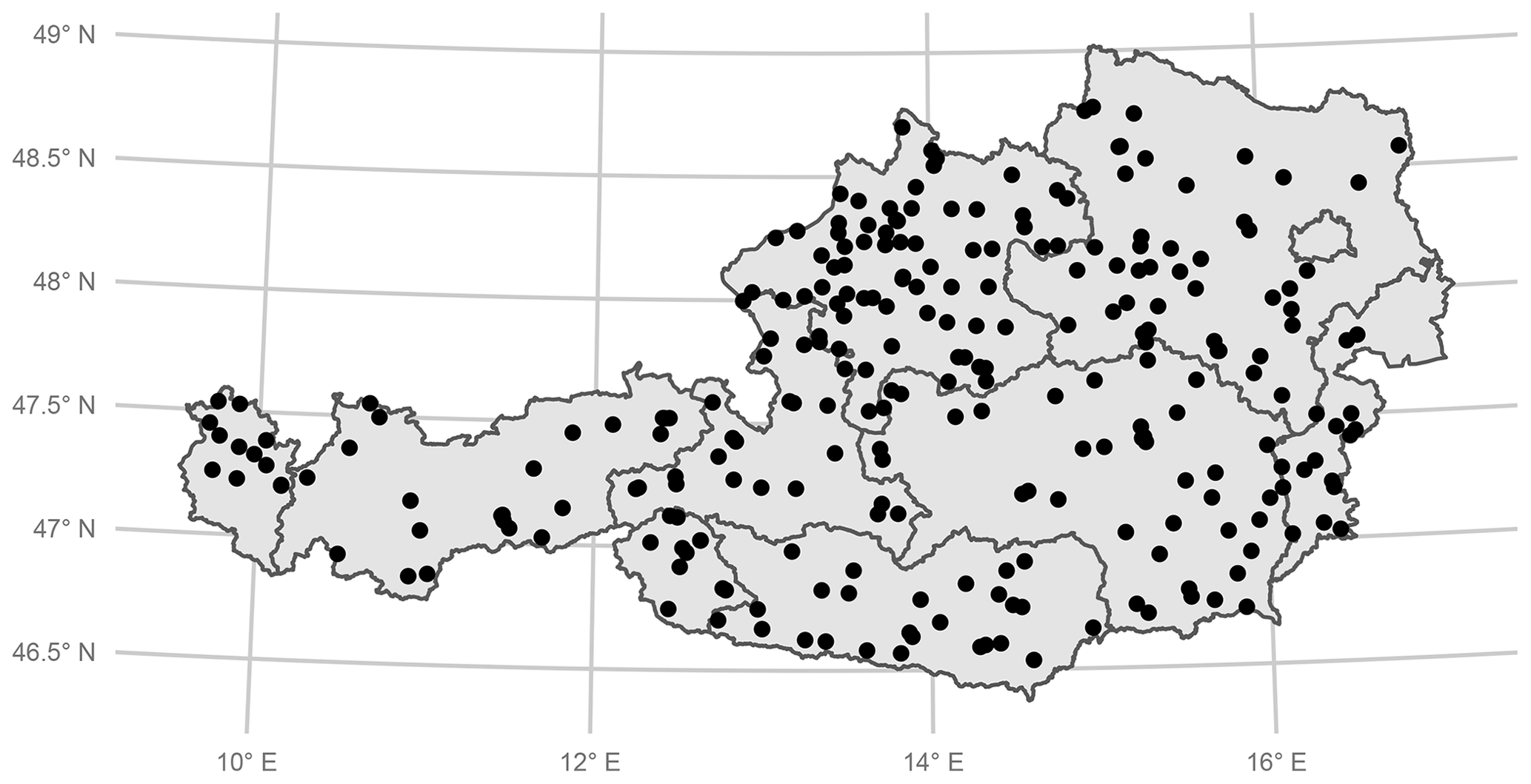
Figure 1Overview of the 260 gauging stations used in the study.
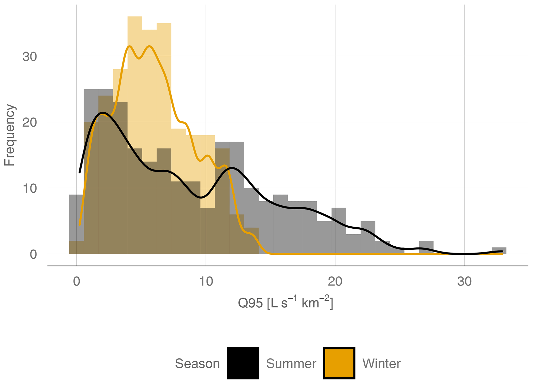
Figure 2Absolute frequency (histogram and kernel density estimate) of summer q95 and winter q95 for all 260 stations.
2.1 Catchment characteristics
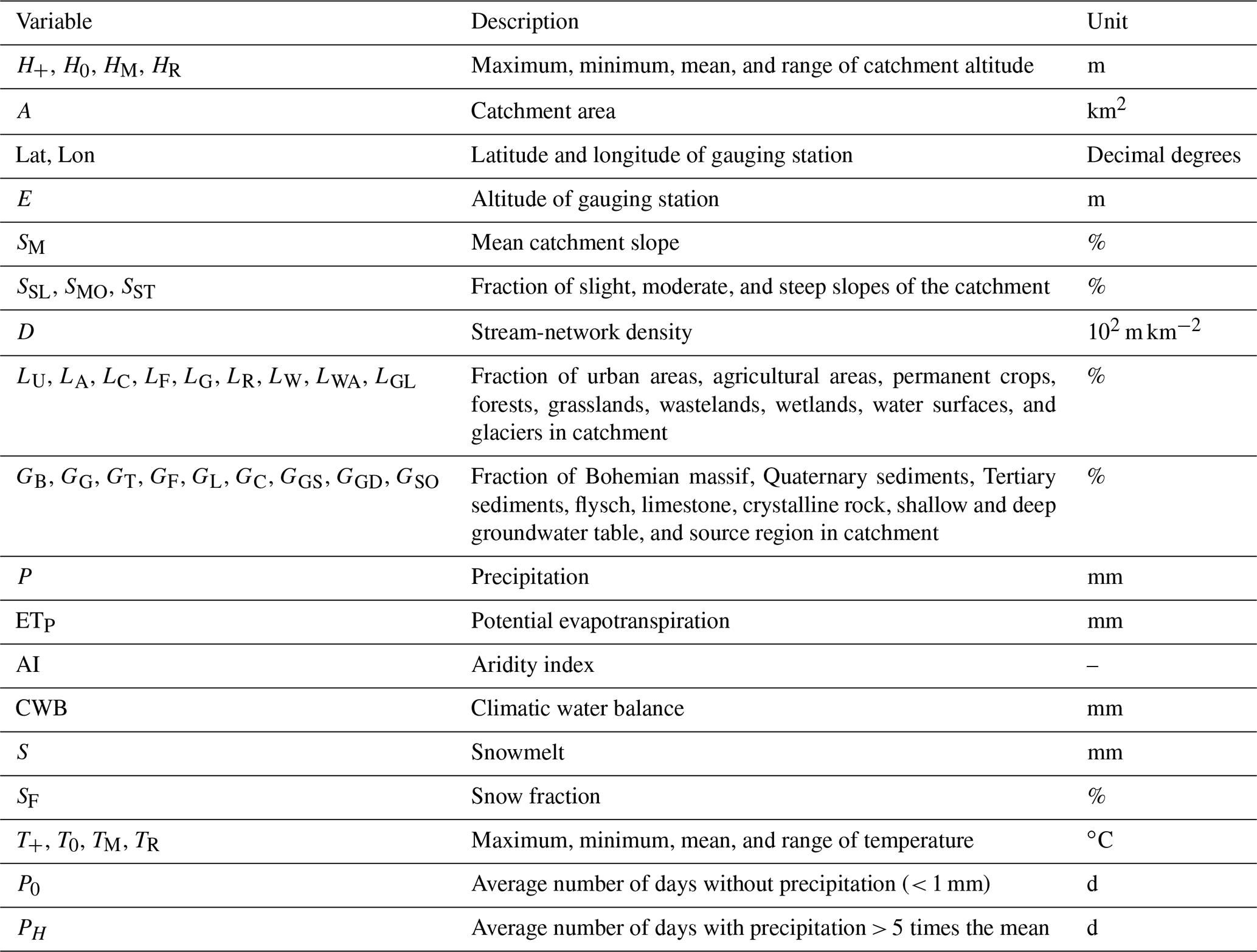
We use a set of 87 covariables as possible predictors, some of which are highly correlated. These covariables can be separated into catchment and climate characteristics. The catchment characteristics used in this study are fully described in, e.g., Laaha and Blöschl (2005, 2006). They consist of nine land use categories, nine geological categories, and information about catchment altitude, stream-network density, and steepness of the slope in the catchment. An overview is given in Table 1.
Table 1Descriptions of the catchment characteristics that are used in the study. Abbreviations are further used in plots. Precipitation, climatic water balance, potential evapotranspiration, aridity index, snowmelt, snow fraction, and temperature variables are used on an annual, seasonal, and half-year basis. These different accumulation periods are indicated by an extension of the indices (annual, spring, summer, autumn, winter, winter, hy and summer, hy).
2.2 Climate characteristics
The calculation of the climate characteristics is based on the SPARTACUS dataset for daily precipitation (Hiebl and Frei, 2018) and daily minimum and maximum temperature (Hiebl and Frei, 2016). Data are available from 1961 to 2018, and the spatial resolution is 1×1 km. Additionally, we retrieved the HISTALP dataset of the fraction of solid precipitation (Efthymiadis et al., 2006; Chimani et al., 2011), which has a coarse spatial resolution of 5×5 min and a temporal range from 1801 to 2014. The dataset was not processed for a finer resolution, as it already relies on a statistical relationship of temperature with solid precipitation (Chimani et al., 2011). To calculate specific climatological variables for each gauging station, the nearest grid point to the gauging station, which lies inside the catchment, was used. The gridded datasets were used to calculate precipitation sums and mean, minimum, and maximum temperature. Daily precipitation was further used to estimate the number of days without precipitation for the winter and summer seasons. We defined a day without precipitation if the precipitation sum on this day was below 1 mm. Potential evapotranspiration was calculated after Hargreaves (Hargreaves, 1994) with the SPEI package in R (Beguería and Vicente-Serrano, 2017). Furthermore, climatic water balance, aridity, and the fraction of snow were computed. Snowmelt is approached by a method of Walter et al. (2005), which is included in the R package EcoHydRology (Fuka et al., 2018). All climatological variables were calculated for the period of 1978 to 2013. Our data were restricted up to the year of 2013, as solid precipitation was only available till the end of 2013. For precipitation, climatic water balance, potential evapotranspiration, snowmelt, snow fraction, and aridity, we calculated average annual sums and mean sums for each season and for the winter and summer half-years (November–April, May–October). The number of days without precipitation was calculated for each half-year and averaged over the whole period. Mean, minimum, and maximum temperatures were calculated for the whole year and the winter and summer periods. Finally, we computed the annual temperature range. All variables related to snow (snowmelt and snow fraction) were transformed by the square root.
This section is divided into two parts. The first part considers the seven statistical learning models used for prediction of summer and winter q95. The second part gives a short description of the RFE algorithm and the proposed variable ranking methods. Additionally, there will be an overview of our repeated nested cross-validation scheme.
3.1 Models
We considered seven statistical learning models that can be structured as follows. Two prediction models use dimension reduction: (i) PCR and (ii) sparse partial least squares (sPLS). Additionally, we used two linear models that possess an inherent variable-selection method – (iii) the Lasso and (iv) linear-model-based boosting approaches (GLM). If simple linear terms are not sufficient, we can extend the GLM by nonlinear smoothing functions. This results in the (v) GAM. A maximum likelihood estimation of a generalized additive model in a regional frequency approach for low flow was already adapted by Ouarda et al. (2018). Finally, we use two models that are popular in hydrology: (vi) RF, (Tyralis et al., 2019) and (vii) SVR (Sujay Raghavendra and Deka, 2014).
All the models can be considered regression models where the response variable Y is a vector of length N(N=260) catchment observations, which can either be summer q95 or winter q95. The predictor matrix X is a N×p matrix with elements xij representing the values of p=87 numeric predictors for the ith catchment.
3.1.1 Lasso
Lasso was originally introduced by Tibshirani (1996), where the regression coefficients βlasso can be defined as follows:
with β0 as the intercept and βj as the regression coefficients. The Lasso model performs a penalized model optimization known as L1 regularization that reduces parameters and shrinks the model. A tuning parameter lambda controls the strength of the penalty and thus the parsimony of the model. Setting lambda to zero results in the ordinary least squares regression estimates, whereas large values of lambda lead to a simple intercept model. In between these limits, lambda performs a continuous subset selection (Hastie et al., 2009). We use the glmnet package in R for computation (Simon et al., 2011), where the coefficients are estimated by cyclical coordinate descent (Friedman et al., 2010). An optimal solution for lambda is chosen by 10-fold cross-validation, where we choose lambda by the 1 standard error rule. We prefer this over using lambda with minimum error, as this results in sparser and more robust models in our case. The Lasso approach can handle high correlated data, coefficients can be shrunk to zero, and correlated variables do not enter the final model (Friedman et al., 2010).
3.1.2 PCR
PCR is a regression method that can deal with multicollinearity and high-dimensional data. PCR projects the predictor matrix X on an orthogonal space, which ensures that the final predictors are uncorrelated. The final dimension of our regression problem can thus be reduced from p (number of predictors) to M (number of principal components). Using M=p would result in the least squares estimate for the full parameter space. The principal components of X are defined as zm=Xνm, where zm are the principal components and νm are the principal directions of X. The final regression coefficients of the principal components (zm) can be defined by Hastie et al. (2009)
where θm is . As for Lasso, X has to be standardized in PCR before estimating the regression coefficients, as the principal components are dependent on the scaling of the initial variables. The number of principal components M is optimized by a 10-fold cross-validation and the regression coefficients are estimated by ordinary least squares. We fit our PCR model using the pls package in R (Mevik et al., 2020).
3.1.3 sPLS
Additionally to Lasso and PCR, we propose a third-dimension reduction method, partial least squares regression (PLS). PLS uses linear combinations of X for the regression of Y, but these linear combinations are now constructed in dependence on Y (Hastie et al., 2009). This overcomes the drawback of PCR, which cannot guarantee that the first principal components of X are most suited to predicting Y. PLS, originally developed by Wold (1966), is an iterative process that starts with centering the response variable (U1) and the predictor variable (V1j). Next, p univariate regression models are constructed by regressing U1 against each centered predictor variable V1,j, which gives us p regression coefficients. These regression coefficients are now used to compute the first PLS component, which is the weighted average defined as
where bj are the univariate regression coefficients defined as , and the weights are wi=Var(V1j). In a next step U2 is estimated by computing the residuals of the regression model U1∼T1. Furthermore, the predictor matrix V2j is updated by the residuals of the models V1j∼T1, where each predictor variable is regressed against the first PLS component. This process is repeated until M PLS components are extracted (de Jong, 1993). As PLS yields a high variability in the performance evaluation, we used an adapted PLS procedure, which is called sPLS. This method was introduced by Chun and Keleş (2010) and includes a variable selection, as an L1 penalty is added to the calculation of the PLS components. The model is tuned by 10-fold CV in the spls package in R (Chung et al., 2019).
3.1.4 Linear and nonlinear model-based boosting
In this section the model-based boosting algorithm is presented, which is used for fitting a simple linear model (GLM) and a GAM. Boosting refers to an ensemble learning approach that converts a set of weak models, termed learners, into a strong model with a better model fit. A current approach is functional gradient descent boosting, a stage-wise, additive approach, which improves a fitted model by adding, each step, a new learner that reduces the model errors. When predictors X are entered as separate learners, so that the prediction function f is an additive estimate based on simple linear terms fj(xj)=βjxj, the approach allows one to obtain an inherent variable selection and can penalize regression coefficients (Mayr and Hofner, 2018). In addition, model-based boosting can deal with multicollinearity and can handle, e.g., linear, nonlinear, spatial, or random effects (Hofner et al., 2014).
Model-based boosting, as applied in this study, aims to minimize an empirical risk
based on the so-called loss function ρ(y,f) characterizing the inadequacy of the fitted model. For regression problems including GLM and GAM, we use the squared error loss function
which results in a stage-wise least-square minimization of the residuals. The boosting algorithm is an iterative process, with the following steps (Bühlmann and Hothorn, 2007; Mayr and Hofner, 2018; Melcher et al., 2017).
-
In a first step all base learners are defined. A base learner can be a, e.g., linear, nonlinear, spatial, or random effect. The two models used in this study incorporate linear base learners for the linear model (GLM) and linear and nonlinear effects for the GAM. As shown by initial analysis, spatial effects or higher-order interaction effects did not improve the prediction performance, and hence they were discarded from the analysis. Nonlinear effects are modeled as P splines (Schmid and Hothorn, 2008), which are decomposed into an unpenalized linear base learner and a penalized nonlinear base learner, each with 1 degree of freedom. The nonlinear base learner is centered by subtracting the unpenalized linear part. This approach is proposed by Kneib et al. (2009) and Fahrmeir et al. (2004) and offers the possibility of spotting the predictor variables that are added as linear or nonlinear effects. This leads to p+1 (p predictor variables plus one term for an intercept) linear base learners for the GLM and 2p+1 base learners for the GAM.
-
In the first iteration, the counter m, which is the number of boosting steps, is set to 0 and the initial function estimate is set to . The first function estimate is determined by an offset, which is the mean of the response for our purpose ().
-
The following steps are now repeated until the maximum number of boosting steps is reached, which was fixed to 1000 in this study.
-
The tuning parameter m is increased by 1.
-
The negative gradient is computed and evaluated at the function estimate of the previous iteration f[m−1], resulting in the negative gradient vector u[m].
-
Each base learner is now fitted by univariate regression against u[m], and the best-fitting base learner is selected.
-
The function estimate is updated by , where ν is a value between 0 and 1, and if ν is sufficiently low, the risk of finding only a local minimum is reduced. Therefore, ν was set to 0.1 in this study.
-
In each boosting step (m>0) only one base learner is selected and can be chosen again in later iterations. The number of boosting steps are optimized by a 10-fold CV. Although studies indicate that repeated CV would yield more robust results (Seibold et al., 2018) due to computational costs, the low risk of overfitting 10-fold CV seemed sufficient. The model boosting was performed using the mboost package in R (Hothorn et al., 2021).
3.1.5 RF
RF is a bagging (bootstrap aggregating) method originally developed by Breiman (2001). In a RF model multiple regression trees are generated using bootstrap samples, and their predictions are averaged to yield the RF estimate. Bootstrapping decorrelates the individual trees and adds some randomness to the predictions. There are several packages in R that can estimate RF models, but due to the computational burden of the study we used the fast ranger package (Wright and Ziegler, 2017). An RF model has several hyperparameters that can be tuned. The number of trees used for bagging is one of these parameters, but it just has to be sufficiently high, as more trees normally do not impair the prediction performance. In this study we used 500 trees. Another parameter that needs to be optimized is the size of each bootstrap sample. We used a grid search from 0.7 to 0.9 for finding an optimal sample size for each bootstrap sample. Sampling was applied without replacement. Further, the number of variables that are randomly chosen for each split needs to be set, which was determined by . We used the estimated response variance as a splitting criterion because rank-based approaches or the use of extremely randomized trees (Geurts et al., 2006) did not improve prediction accuracy.
3.1.6 SVR
Support vector machines have their origin in classification but can be extended to regression problems. The method in its basic form uses a training dataset to create a line (or hyperplane) that separates the data into classes. The support vectors are the data points closest to the line or hyperplane and have the most influence on parameter estimation. In SVR, each of the predictor variables can be transformed to a set of basis function hm(xj). Hence the regression function f(x) can be approximated by (Hastie et al., 2009)
The number of M basis functions is not limited, and to estimate the coefficients β0 and βm, H(β,β0) has to be minimized:
V can be any loss function, but in the initial idea of Vapnik (2000), it is defined by a threshold r. If the residuals are higher than this value, they are included in the penalization of the model, and if the residuals are lower, they are discarded (Worland et al., 2018). Hence, the SVR is insensitive to outliers, as coefficients will be penalized with respect to them. The fast computation of the coefficients is achieved by only computing the inner product of each xj. Therefore, different kernels can be used, and we decided to use the nonlinear radial kernel in our study. The SVR model was estimated by the e1071 package in R (Meyer et al., 2021).
3.2 Variable preselection for parsimonious models
The variable selection procedure of this study is based on the recursive feature elimination (RFE) algorithm. RFE is a prospective method that initially ranks the predictor variables after some measurements of importance, and the least important variables are removed in a backward procedure (Granitto et al., 2006). The final number of variables are determined by an error measurement of an independent test set. In this part we will present our three approaches for variable ranking, the error measurement to define the number of variables, and a short overview of the validation scheme.
3.2.1 Variable ranking methods
We test three different methods for the variable ranking of the RFE. Thus, we can differentiate between the prediction accuracy of the prediction models and the capability of different variable ranking methods for producing more parsimonious models.
-
The first variable ranking method is Lasso (lassorank), which is applied as described in Sect. 3.1.1, except that standardized coefficients are calculated.
-
Second, we use a linear model-based boosting approach (glmrank). Every model is estimated by 500 boosting steps, since boosting shows only slow overfitting behavior (Fig. 3). One disadvantage is that some non-influential variables will be ranked, but computation time is reduced. For calculation of the standardized coefficients we apply the variable importance function of the caret package in R (Kuhn, 2021).
-
The third method (cfrank) uses conditional forests (Hothorn et al., 2006; Strobl et al., 2007, 2009) for variable ranking, where the standardized coefficients are a sum of the main and interaction effects for each variable. Standardized coefficients are again calculated using the variable importance function of the caret package.
Our variable ranking is computed over a bootstrap sample to improve its robustness with respect to data. Therefore, an initial dataset D is split up into 25 bootstrap samples (). Sampling is performed without replacement, and a sample size of 68.2 % is used.
In a next step, each of the bootstrap samples is fitted to one of the variable ranking methods. For each bootstrap sample and each method, standardized coefficients denoted as are returned, where b refers to the bootstrap sample, method is the variable ranking method (lassorank, glmrank, cfrank), and j is the considered predictor. The variable importance of each bootstrap sample for each selected coefficient is calculated by
Final variable rankings are computed by averaging over all 25 bootstrap samples (Eq. 9). The variables are ranked from highest to lowest.
Variables that were never selected in the 25 bootstrap samples are not considered for the variable selection. This yields nvar preselected variables for each method.

Figure 3Prediction error for the unseen test data (a) and the training data (b). Bootstrapping was performed 100 times where the training set consists of 70 % of the observations.
3.2.2 Model-specific preselection of variables
The variable rankings are now calculated for each of the seven prediction models. Each prediction model is fitted to the best l () ranked variables, and for each prediction vector the RMSE as a measure of fit is calculated:
As one aim of this study is to get unbiased predictions (Solomatine and Ostfeld, 2008; Ambroise and McLachlan, 2002), we employ a nested CV scheme (referred to as double CV in Varmuza and Filzmoser, 2016). The nested 10-fold CV consists of two loops, where the inner loop is used for model optimization and variable selection and the outer loop is used for independently evaluating the predictive performance of the so-obtained models. In the outer loop the data are split into 10 folds, 9 of which define the calibration data and the remaining 1 the test data. The calibration data are sent to the inner loop, where again these data are split into 10 folds, 9 of which are used for variable rankings and parameter estimation. The left-out fold is used for estimating the RMSE for each candidate variable selection (l). The RMSEl is then simply averaged over the 10 folds of the inner CV. The final number of variables (nfinal) of a method is then obtained from the relationship of the RMSEl vs. the number of variables l, as exemplified in Fig. 4. A common option is to use the min(RMSE) for determining nfinal, but this would only yield a small reduction in the number of variables. We therefore propose using a somewhat (+5 %) higher residual error, i.e., , as the reference point. This should make the models more parsimonious with only a slight loss in performance. In a final step, we determine the specific variables that are used for predictions of the outer loop of the nested CV. For this we use all obtained variable rankings of each of the 10 inner folds of the CV run and average each variable ranking over these 10 folds. The best nfinal variables of these final rankings are used for prediction. The process is repeated 10 times for the outer loop to complete the cross-validation.
The full nested CV is again repeated 10 times for summer q95 and winter q95.
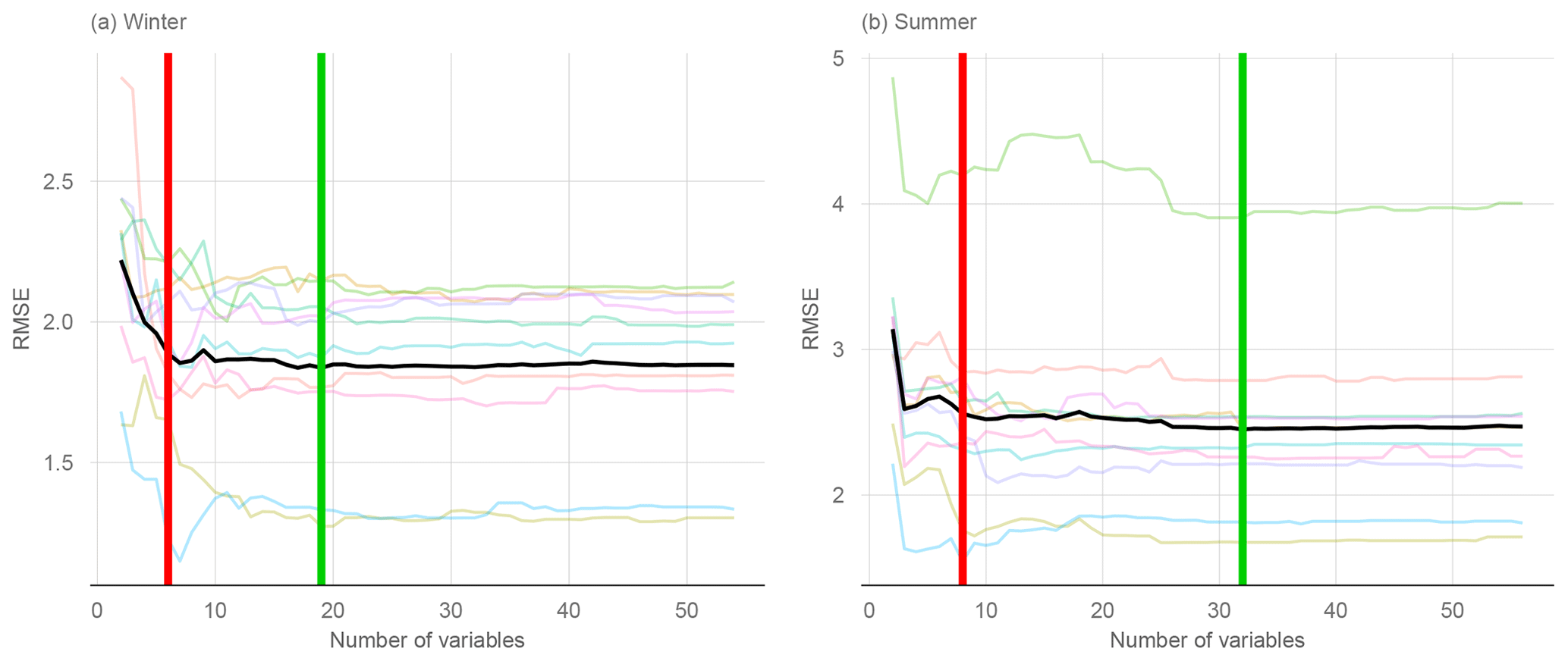
Figure 4Variable selection for a GAM boosting model based on RMSE graphs. The red vertical line indicates the number of variables selected by a 5 % increase in the min(RMSE), and the green line is the number of variables obtained by min(RMSE). The black graph is the average over 10 inner CV folds, and colored graphs represent individual folds.
3.2.3 Performance evaluation metrics
Model evaluation was performed by the RMSECV and the relative root mean squared error RRMSECV of each CV repetition:
where is the mean of all observations. We further compare our results by the cross-validated defined as
For a more focused assessment of individual catchments in terms of how CV performance depends on climate and catchment characteristics, we use the absolute normalized error ANECV of the ith catchment:
4.1 Model performance without variable preselection
Figure 5 shows the performance of all the models without variable preselection and Table 2 presents the performance metrics of all the models. The best-performing model for winter low flow is the SVR model with a median of 0.70 over all 10 CV runs. It is followed by the GLM (0.69) and RF (0.68) and a group of similarly performing models (Lasso, GAM, PCR, and sPLS), with an of 0.66. Summer low flow generally reaches a higher prediction accuracy, with a of 0.86 (GAM) and 0.85 (GLM) for the two boosting approaches and a somewhat lower performance for Lasso, sPLS, RF, SVR (all 0.84), and PCR (0.83).
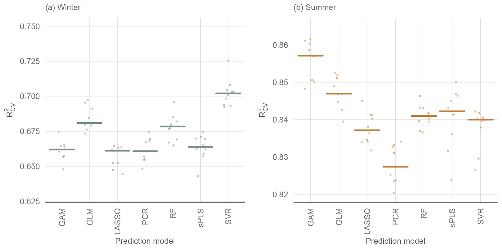
Figure 5Performance of 10 CV runs of statistical learning models without variable preselection. Horizontal lines display the median of the CV runs.
Additional insights can be gained by stratifying the predictions by specific low-flow magnitude into three parts, the first part containing observations smaller than the first quartile, the second part ranging between the first and third quartiles and the third part considering only the observations higher than the third quartile. For each of the three parts we calculated the RRMSECV. High q95 winter values reach similar performances for all the models, with a RRMSECV of 0.24 to 0.25. Middle-ranged values are best approximated by the Lasso model (RMSErel=0.24), followed by the RF and the SVR (both 0.25) and slightly worse performances by the two boosting models (0.26) and sPLS and PCR (0.27). The main differences between the model predictions can be observed for the lowest observation class, where the SVR model with a RRMSECV of 0.58 performs substantially better than the other models. The next best model in this class is the GLM (0.66), and models such as RF (0.75) and GAM (0.78) have less prediction accuracy.
For summer low flow, low q95 values again have a higher relative error than medium or high q95 values. For the lowest observation quartile, the GLM shows the best performance (RRMSECV of 0.49) compared to most other models (RRMSECV between 0.54 and 0.56). The sPLS (0.62) and the RF (0.71) show a much lower prediction accuracy in this class. Differences for moderate summer q95 values are only marginal, with a range of 0.3 (SVR) to 0.32 (PCR). High summer q95 values are somewhat better approached by the GAM (0.2), with a slightly higher RRMSECV of all other models ranging from 0.21 to 0.23.
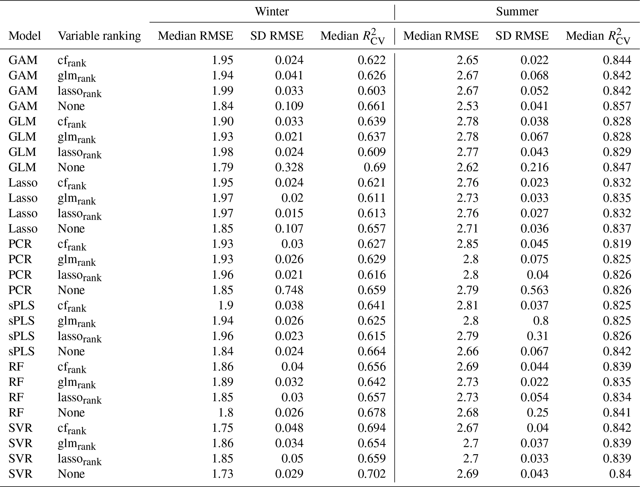
Table 2Overview of the prediction performance of all the models. The median and standard deviation (SD) are calculated over the 10 CV runs for each model.
4.2 Effect of variable preselection
The use of variable preselection can significantly reduce the complexity of all the models, with only a small loss of performance (Fig. 6). For winter low flow, variable selection leads to a median decrease of 5.1 % (cfrank), 5.8 % (glmrank), and 7.1 % (lassorank) over all the models. The spread in performance across models is a bit higher for lassorank, with an interquartile range (IQR) of 4.1 % compared to an IQR of 3 % for cfrank and 2.8 % for glmrank. Although cfrank yields a slightly better performance than glmrank and lassorank, the conditional forest approach requires 35 variables, where glmrank and lassorank only use 12 and 14 variables for winter q95. glmrank and lassorank are therefore much more effective. The number of variables for the three variable ranking methods have almost no dispersion, with an IQR of 1 (glmrank), 2 (cfrank) and 3.5 (lassorank). Interestingly, the highest performance loss is observed with the linear boosting model (GLM) for all three variable ranking methods. This is due to the nature of boosting methods, whose main strength is efficient parameter estimation for high-dimensional multicollinear datasets. Clearly, variable preselection affects the performance of the method. In contrast to winter low flow, where the performance loss corresponds well to the +5 % residual error specification, variable selection for summer low flow only leads to a minor loss in performance (Fig. 6b). Here, the median decrease is only 1 % for cfrank and lassorank and 0.8 % for glmrank. Also, the differences between models are very small. Again, cfrank yields a substantially higher number of variables (22) than the glmrank method (8) and lassorank (9). Furthermore, the IQR of the number of variables shows that the selected number of variables is about the same in all the models for lassorank (IQR = 3) and glmrank (IQR = 2) but greatly differs between the models based on cfrank (IQR = 23). This spread reflects a much lower parameter-reduction efficiency of cfrank for the linear models (22 predictors for PCR, 35 for lasso, 42 for sPLS, 50 for GLM) than for the nonlinear models (12 predictors for RF, 17 for SVR, 18 for GAM). Among all the models, the RF provides the model with the lowest number of variables for summer low flows. It consists (on median) of only three variables when lassorank and glmrank are used for variable selection and has a performance loss of less than 1 %.
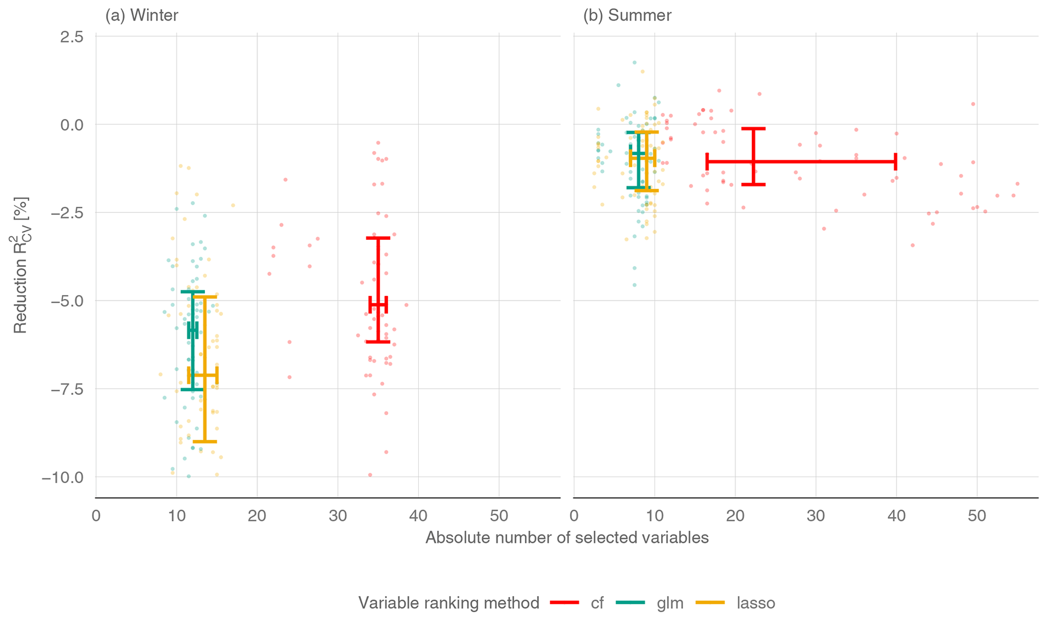
Figure 6Reduction of is computed with respect to the model performance without any variable preselection. Each point is the median number of variables of one CV run and one prediction model and the related . Each line shows (horizontal: number of variables, vertical: reduction in ) the upper and lower quartiles for a variable ranking method. Colors can be found in Ram and Wickham (2018).
4.3 Importance of predictors (from variable rankings)
We performed variable rankings for each of the three ranking methods 1000 times inside the CV runs. In this section we discuss the 10 best-ranked variables for each variable ranking method, defined by the average rank over all 1000 repetitions. We focus on the two linear ranking methods, as the nonlinear method cfrank did not perform well.
Figure 7 gives an overview of the rank counts for winter low flow and shows that the catchment altitude is on average the highest-ranked variable. Meteorologically based variables appear four (glmrank) and five (lassorank) times among the 10 best-ranked variables. Predictors rated by both methods are aridity and snowmelt in the winter months. glmrank lists preconditions such as precipitation or dry days in the summer as important variables. However, lassorank found dry days in winter and over the whole year to be more important. Geological variables such as percentage of Quaternary sediments or limestone enter the models as indicators for catchment processes. Finally, land use characteristics such as proportion of agriculture area and wasteland rocks were found for glmrank, where only the fraction of grassland is rated by lassorank. Both are correlated with the proportion of lowland/high mountain areas and can be interpreted as topological characteristics as well.
A slightly different picture emerges from the assessment of summer low flow (Fig. 8), where the three highest-ranked variables are maximum catchment altitude, mean catchment slope and dry days in summer for both variable ranking methods. Topological descriptors play a somewhat more dominant role for summer low flow, as four (glmrank) and five (lassorank) variables are highly ranked. Apart from mean catchment slope and maximum catchment altitude, difference in catchment altitude and stream-network density are also found for both variable ranking methods. Two meteorological variables – aridity in winter (both methods) or autumn (lassorank) and the annual temperature range (lassorank) – are found by each of the methods for summer q95 in addition to the dry days in summer. Finally, geological features such as the proportion of flysch or land use variables such as the fraction of grassland are highly ranked for both approaches.
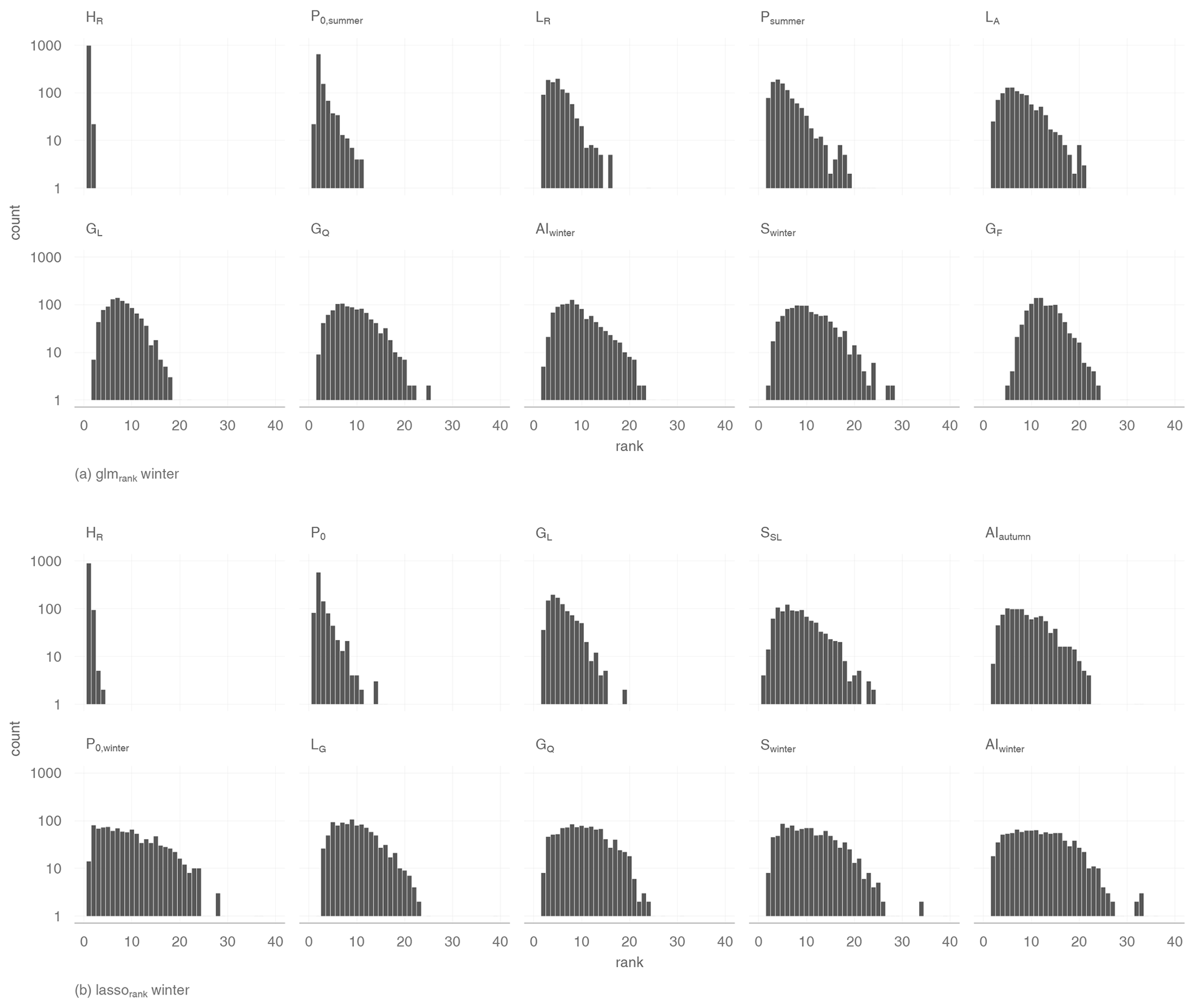
Figure 7Count of all variable rankings of all 1000 iterations on a log scale for winter low flow. The 10 best variables are listed after their averaged rank.

Figure 8Count of all variable rankings of all 1000 iterations on a log scale for summer low flow. The 10 best variables are listed after their averaged rank.
5.1 Predictive performance and benchmarking
We showed that statistical learning models can yield high prediction accuracy. It is now interesting to assess how the models fit into the picture of existing national and international studies. We first assess the performance relative to low-flow regionalization studies for the Austrian study area. Laaha and Blöschl (2006) fitted a multiple-regression model to annual low-flow q95 on 325 (sub-)catchments. They reported a performance of when the study area was subdivided into regions that exhibit similar seasonal characteristics of low flow. In a subsequent study, Laaha et al. (2014) showed that top kriging can outperform regional regression, especially when interpolating between gauges at the larger rivers. Top kriging (TK, Skøien et al., 2006) is a geostatistical method that uses stream-network distance for low-flow prediction and was shown to be more adequate than ordinary kriging approaches. For comparison of our results with the current benchmark (TK), we used the same 10-fold CV runs as for our statistical learning models. TK yields a median of 0.68 for winter low flow, which is slightly below the SVR and the GLM and equivalent to the RF model. TK performs similarly to most models for summer q95, with a median of 0.84, and performs quite similarly to the two boosting approaches. Hence, we show that statistical learning models can perform as well as or even better than the current benchmark TK for summer and winter low flow in the Austrian study area.
It is also interesting to compare our findings to existing studies that assess statistical learning methods for low-flow estimation. However, comparison of performance metrics across studies is not straightforward. Worland et al. (2018) and Ferreira et al. (2021) assessed their prediction models for low-flow characteristics such as Q95 and a quite similar characteristic 7Q10, but these were not standardized by catchment area as in our study. This can lead to superior performance metrics, particularly if there are significant variations in catchment size within the sample. Worland et al. (2018) reported a Nash–Sutcliffe efficiency (NSE) (which is equivalent to the in this study) of 0.92 for the meta M5-cubist model, and Ferreira et al. (2021) reported a NSE value of almost 1. However, the scatterplots of the studies suggest that errors are still considerable, especially for the low observation values. Although the studies are not directly comparable to our study in terms of performance, a qualitative comparison is still warranted. Both studies found tree-based methods, including the ensemble M5-cubist model (Worland et al., 2018), the RF (Zhang et al., 2018), and tree-based boosting (Tyralis et al., 2021) with a higher prediction accuracy than the other models. Our study complements existing studies by examining additional learning models. Our results suggest that the SVR and the GAM boosting model can outperform tree-based models for the Austrian setting. However, differences in performance are rather small, so that other methods (e.g., GLM, lasso, and tree-based RF) can also be considered well suited.
One major research gap addressed by this study is the separate evaluation of statistical learning models for seasonal low-flow processes. All statistical learning models of this paper can be classified as global models, as all gauges are considered in the same model without catchment grouping. Earlier studies showed that regional regression can increase the prediction accuracy compared to global regression (Laaha and Blöschl, 2006, 2007) as different low-flow generation processes apply to summer and winter regions. Here we pursue a different strategy in which we separate summer and winter processes by a temporal stratification into summer and winter low flows. We found that analyzing winter and summer low-flow indices individually leads to increased prediction accuracy, especially for summer q95. This emphasizes that prediction accuracy of a specific model is influenced by the underlying hydrological process, and different models can be suitable for different applications (Worland et al., 2018). For comparison, preliminary results without consideration of the seasonal regime of our study area have led to a prediction accuracy of a median () of 0.66 to 0.74 which is very similar to the earlier studies on annual low flow (TK 0.75).
5.2 Predictive performance as a function of catchment characteristics
In a comparative assessment of low-flow studies based on the PUB assessment report (Blöschl et al., 2013), Salinas et al. (2013) showed that prediction accuracy is not only a function of model selection, but also of the specific setting of the study area. The assessment did not contain statistical learning models, so we want to embed our results in their findings. Figure 9, which is equivalent to Fig. 5 of Salinas et al. (2013), shows the ANECV as a function of the aridity index, the catchment area and the catchment altitude. Our study confirms the finding of the PUB assessment report that the prediction accuracy decreases as the aridity of the study area increases (Salinas et al., 2013). Although stations with an aridity index over 1 are missing, the trend is clearly evident. No trend is evident for the winter low flows, which are more driven by freezing processes than by a climatic water balance deficit. Decreasing performance in arid regions for drought detection was also found by Haslinger et al. (2014). This effect may be additionally intensified because in arid regions the mean of observations can be near zero.
Another hypothesis of Salinas et al. (2013) is that a higher elevation increases the prediction accuracy. In this context we found remarkably divergent results for summer and winter low flow. Whereas our findings for summer low flow are in line with Salinas et al. (2013), we could not identify a clear tendency for winter low flow. Catchments located in lowlands and mountainous areas have a somewhat larger ANECV than catchments with an elevation between 450 and 1500 m. This suggests that winter low flows are more predictable in colder mid-mountain catchments than in warmer lowland catchments, where occurrence of frost events varies from year to year. Finally, we can show that prediction accuracy is increasing with catchment size, which is fully consistent with Salinas et al. (2013).
Another finding of (Salinas et al., 2013) that is not captured by Fig. 9 is that predictions of low flows in cold climates are reaching a lower prediction accuracy than in humid and thus warmer climates. A comparable effect can be observed when comparing the results for winter low flow and summer low flow, where the best-performing model in winter has a of 0.70 and 0.86 in summer. This divergence can be explained by the more complex hydrological processes of winter low flows (Salinas et al., 2013). It is shown here that this performance gap applies to seasonal climates with a warm season and a frost period in the same way as between cold and humid climates.
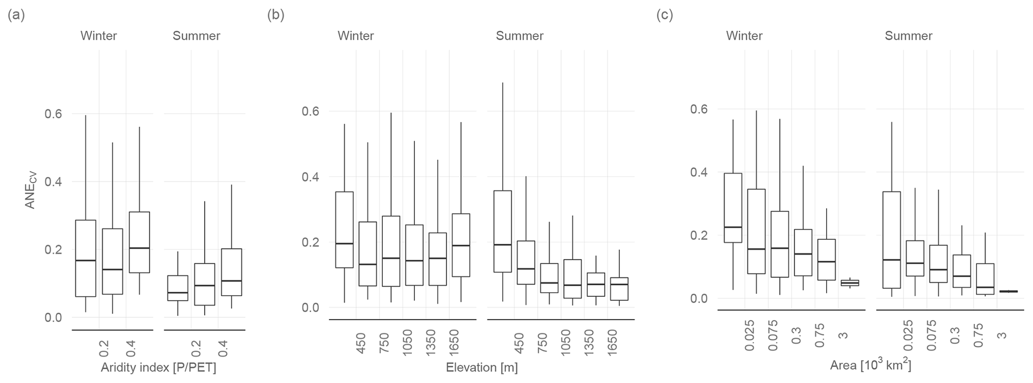
Figure 9ANECV for summer and winter q95 as a function of the aridity index (a), elevation (b), and catchment area (c). Only the best-performing models are shown (winter SVR, summer GAM, both without variable preselection). The box plots summarize the ANECV averaged over all 10 CV runs for each of the 260 stations.
5.3 Linear vs. nonlinear models
All studies that conducted a comparative assessment of statistical learning models for low-flow estimation highlighted that nonlinear models are superior with respect to linear approaches (e.g., Worland et al., 2018; Ferreira et al., 2021; Zhang et al., 2018; Tyralis et al., 2021). In principle this is consistent with our findings, where winter low flow is best predicted by the SVR model and summer q95 is best approached by the GAM model. However, we showed that linear statistical learning models such as GLM or sPLS perform almost as well in our study. To shed more light on this issue, we assessed the relative value of the GAM over the GLM boosting model in more detail. Both models are equivalent in case of linear relationships, but the GAM offers the possibility of extending the GLM with nonlinear relationships if these improve the model. The comparison shows that the GAM is selecting additional nonlinear effects to increase the goodness of fit. However, the additional effects do not increase the predictive performance of the model. In fact, the of the GAM is only 1 % higher for summer but 3 % lower for winter low flow when using the model without variable preselection. This suggests that nonlinear processes, which are to be expected in such a heterogeneous study area as Austria, can be sufficiently captured by the superposition of linear terms, so there is no need to add nonlinear effects or to use a nonlinear model. This is additionally supported by the performance of the three variable ranking methods. The nonlinear approach of conditional forest leads only to a small reduction of the set of predictors, with performance similar to (winter q95) or worse than (summer q95) the two linear ranking methods.
In this study we investigated a broad range of statistical learning methods for a comprehensive dataset of 260 catchments in Austria. The results showed that all statistical learning models perform well and are therefore well suited for low-flow regionalization. Performance is particularly high for summer low flow () but still leads to satisfactory results for winter low flow (). The best-performing models are support vector regression (winter) and nonlinear model-based boosting (summer), but linear models exhibit similar prediction accuracy. No superior model could be found for either low-flow process, as relative differences between learning methods are actually small. The models perform similarly to or slightly better than a top-kriging model that constitutes the current benchmark for the study area.
Variable preselection is shown on average to reduce the predictor set (on median) from 87 variables to 12 for winter and 8 for summer low flow. This is achieved by a small loss in performance, which is about 5 % for winter low flow and only 1 % for summer low flow. The results suggest that variable preselection can help to create parsimonious learning models that are easier to interpret and more robust when predicting at ungauged sites. The RF (summer) provides the model with the smallest number of predictors, which consists of only three variables and has a performance loss of less than 1 %.
Linear prediction models such as the linear model-based boosting reveal high prediction accuracy. Nonlinear terms were shown to increase the goodness of fit of the models but did not improve predictions at ungauged sites. Our results suggest that nonlinear low-flow relationships can be sufficiently captured by linear learning models, so there is no need to use more complex models or to add nonlinear effects. This finding is confirmed by our variable ranking methods, where linear approaches seem to be sufficient for our estimation problem.
Variable rankings allow some conclusions about the importance of predictor variables. Topographic variables representing altitude and slope are among the most highly ranked predictors for summer and winter low flows. Specific low flow is mainly increasing with topographic predictors, except that the percentage of slight slope in the catchment has a decreasing effect. Among meteorological predictors, characteristics representing snowmelt, aridity, and dry spells appear more important than precipitation characteristics. The aridity and number of dry days reduce specific low flow, whereas snowmelt has an increasing effect. The best-rated geological characteristics are the area fractions of limestone, flysch and Quaternary sediments. Limestone and Quaternary sediments both lead to higher low flows, whereas flysch has a decreasing effect. Overall, topological, meteorological and catchment characteristics appear similarly important for low-flow regionalization. However, the interpretation of the variable ranking should be considered with caution as substituting top-ranked variables in highly correlated data can lead to similar performance.
Finally, the study shows that when performing low-flow regionalization in a seasonal climate with a cold winter season, the temporal stratification into summer and winter low flows increases the predictive performance of all learning models. This suggests that conducting separate analyses of winter and summer low flows provides a data-efficient alternative to catchment grouping that is recommended otherwise.
Figure A1Error bars showing the range of predictions of the 10 CV runs for each model without variable preselection. Two outliers are not shown for the summer PCR model and the winter GLM, PCR, lasso, and GAM models to improve visual clarity.
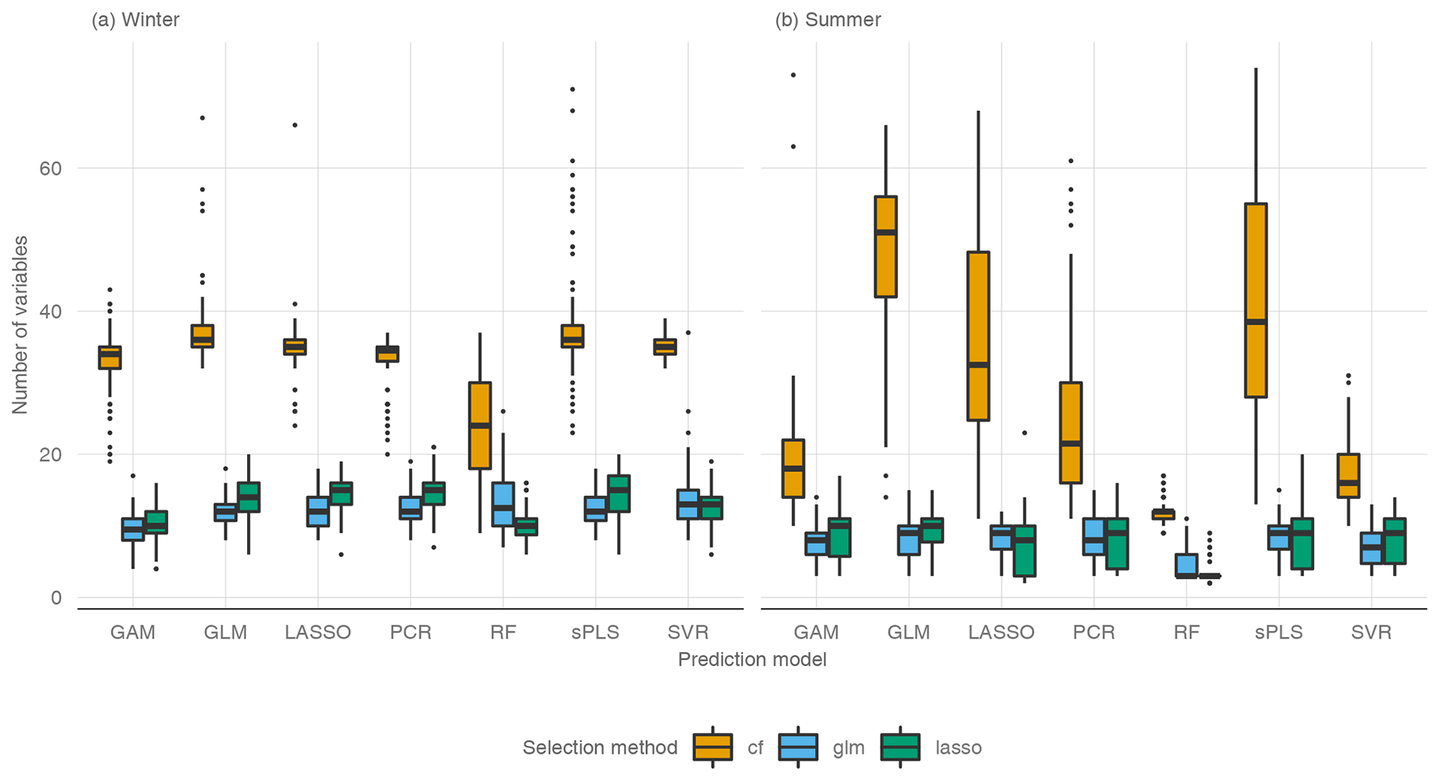
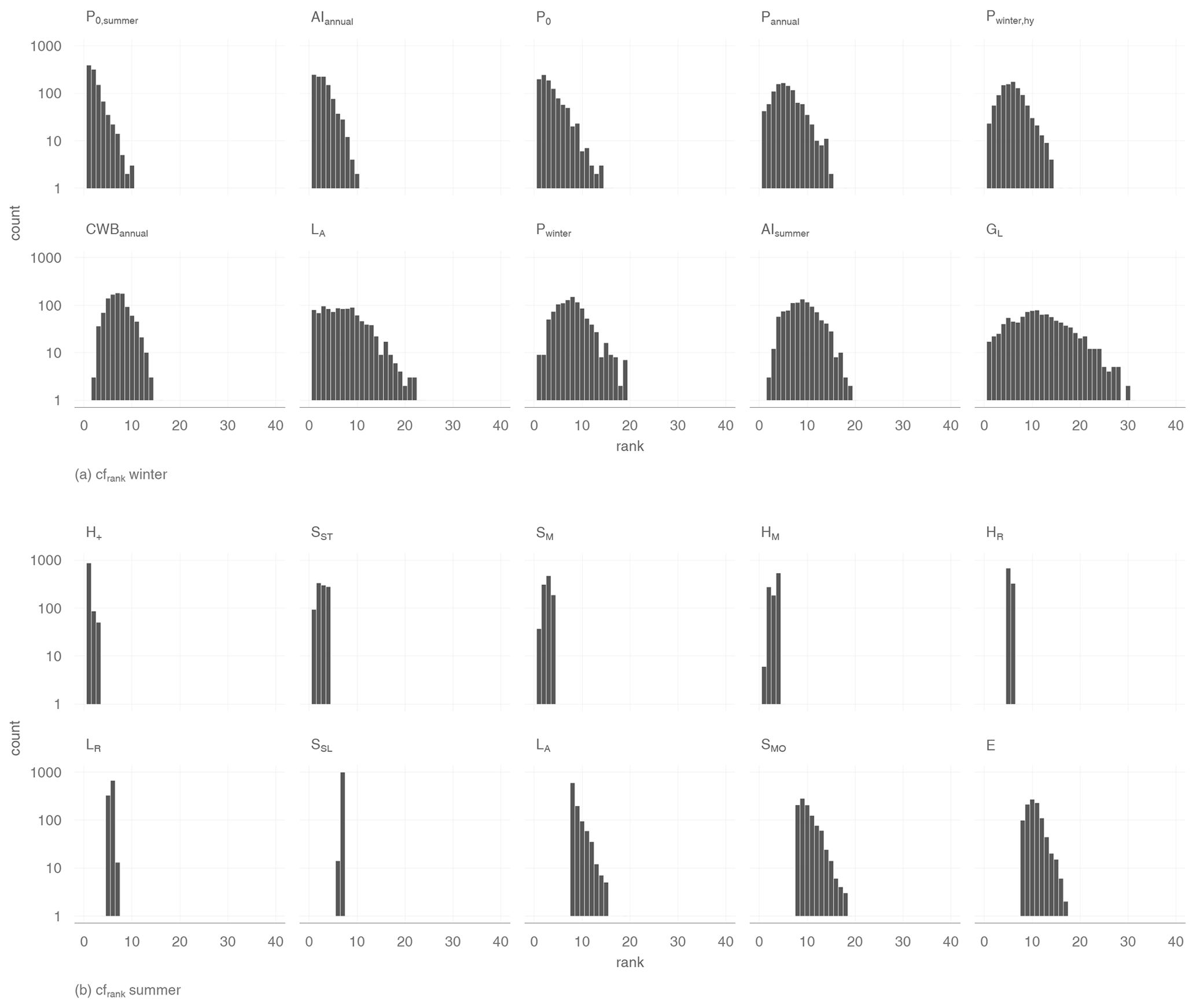
Figure A3Count of all variable rankings of all 1000 iterations on a log scale for summer low flow. The 10 best variables are listed after their averaged rank.
Data and code can be made available on personal request to johannes.laimighofer@boku.ac.at.
JL designed the research layout and GL contributed to its conceptualization. JL performed the formal analyses and prepared the draft paper. MM supported the analyses. GL supervised the overall study. All the authors contributed to the interpretation of the results and writing of the paper.
The contact author has declared that neither they nor their co-authors have any competing interests.
Publisher’s note: Copernicus Publications remains neutral with regard to jurisdictional claims in published maps and institutional affiliations.
Johannes Laimighofer is a recipient of a DOC fellowship (grant number 25819) of the Austrian Academy of Sciences, which is gratefully thanked for financial support.
Data provision by the Central Institute for Meteorology and Geodynamics (ZAMG) and the Hydrographical Service of Austria (HZB) was highly appreciated. This research supports the work of the UNESCO-IHP VIII FRIEND-Water program.
We also want to thank Kolbjorn Engeland and an anonymous reviewer for their valuable comments and Rohini Kumar for handling the manuscript.
This research has been supported by the Österreichischen Akademie der Wissenschaften (grant no. 25819).
This paper was edited by Rohini Kumar and reviewed by Kolbjorn Engeland and one anonymous referee.
Abrahart, R. J., Anctil, F., Coulibaly, P., Dawson, C. W., Mount, N. J., See, L. M., Shamseldin, A. Y., Solomatine, D. P., Toth, E., and Wilby, R. L.: Two decades of anarchy? Emerging themes and outstanding challenges for neural network river forecasting, Prog. Phys. Geog., 36, 480–513, https://doi.org/10.1177/0309133312444943, 2012. a
Ambroise, C. and McLachlan, G. J.: Selection bias in gene extraction on the basis of microarray gene-expression data, P. Natl. Acad. Sci. USA, 99, 6562–6566, https://doi.org/10.1073/pnas.102102699, 2002. a, b
Beguería, S. and Vicente-Serrano, S. M.: SPEI: Calculation of the Standardised Precipitation-Evapotranspiration Index, r package version 1.7, available at: https://CRAN.R-project.org/package=SPEI (last access: 15 Septepmber 2021), 2017. a
Blöschl, G., Sivapalan, M., Wagener, T., Savenije, H., and Viglione, A.: Runoff prediction in ungauged basins: synthesis across processes, places and scales, edited by: Blöschl, G., Wagener, T., and Savenije, H. Cambridge University Press, https://doi.org/10.1017/CBO9781139235761, 2013. a
Breiman, L.: Random forests, Mach. Learn., 45, 5–32, https://doi.org/10.1023/A:1010933404324, 2001. a
Bühlmann, P. and Hothorn, T.: Boosting algorithms: Regularization, prediction and model fitting, Stat. Sci., 22, 477–505, https://doi.org/10.1214/07-STS242, 2007. a
Castiglioni, S., Castellarin, A., and Montanari, A.: Prediction of low-flow indices in ungauged basins through physiographical space-based interpolation, J. Hydrol., 378, 272–280, https://doi.org/10.1016/j.jhydrol.2009.09.032, 2009. a
Castiglioni, S., Castellarin, A., Montanari, A., Skøien, J. O., Laaha, G., and Blöschl, G.: Smooth regional estimation of low-flow indices: physiographical space based interpolation and top-kriging, Hydrol. Earth Syst. Sci., 15, 715–727, https://doi.org/10.5194/hess-15-715-2011, 2011. a
Chimani, B., Böhm, R., Matulla, C., and Ganekind, M.: Development of a longterm dataset of solid/liquid precipitation, Adv. Sci. Res., 6, 39–43, https://doi.org/10.5194/asr-6-39-2011, 2011. a, b
Chun, H. and Keleş, S.: Sparse partial least squares regression for simultaneous dimension reduction and variable selection, J. Roy. Stat. Soc. B Met., 72, 3–25, https://doi.org/10.1111/j.1467-9868.2009.00723.x, 2010. a
Chung, D., Chun, H., and Keles, S.: spls: Sparse Partial Least Squares (SPLS) Regression and Classification, r package version 2.2-3, available at: https://CRAN.R-project.org/package=spls (last access: 15 September 2021), 2019. a
Dawson, C. and Wilby, R.: Hydrological modelling using artificial neural networks, Prog. Phys. Geog., 25, 80–108, https://doi.org/10.1177/030913330102500104, 2001. a
de Jong, S.: SIMPLS: An alternative approach to partial least squares regression, Chemometr. Intell. Lab., 18, 251–263, https://doi.org/10.1016/0169-7439(93)85002-X, 1993. a
Efron, B.: Prediction, estimation, and attribution, Int. Stat. Rev., 88, S28–S59, https://doi.org/10.1080/01621459.2020.1762613, 2020. a
Efthymiadis, D., Jones, P. D., Briffa, K. R., Auer, I., Böhm, R., Schöner, W., Frei, C., and Schmidli, J.: Construction of a 10-min-gridded precipitation data set for the Greater Alpine Region for 1800–2003, J. Geophys. Res.-Atmos., 111, D01105, https://doi.org/10.1029/2005JD006120, 2006. a
Euser, T., Winsemius, H. C., Hrachowitz, M., Fenicia, F., Uhlenbrook, S., and Savenije, H. H. G.: A framework to assess the realism of model structures using hydrological signatures, Hydrol. Earth Syst. Sci., 17, 1893–1912, https://doi.org/10.5194/hess-17-1893-2013, 2013. a
Fahrmeir, L., Kneib, T., and Lang, S.: Penalized structured additive regression for space-time data: a Bayesian perspective, Stat. Sinica, 14, 731–761, 2004. a
Ferreira, R. G., da Silva, D. D., Elesbon, A. A. A., Fernandes-Filho, E. I., Veloso, G. V., de Souza Fraga, M., and Ferreira, L. B.: Machine learning models for streamflow regionalization in a tropical watershed, J. Environ. Manage., 280, 111713, https://doi.org/10.1016/j.jenvman.2020.111713, 2021. a, b, c, d, e, f, g, h, i
Friedman, J., Hastie, T., and Tibshirani, R.: Regularization paths for generalized linear models via coordinate descent, J. Stat. Softw., 33, 1–22, 2010. a, b
Fuka, D., Walter, M., Archibald, J., Steenhuis, T., and Easton, Z.: EcoHydRology: A Community Modeling Foundation for Eco-Hydrology, r package version 0.4.12.1, available at: https://CRAN.R-project.org/package=EcoHydRology (last access: 15 September 2021), 2018. a
Geurts, P., Ernst, D., and Wehenkel, L.: Extremely randomized trees, Mach. Learn., 63, 3–42, https://doi.org/10.1007/s10994-006-6226-1, 2006. a
Granitto, P. M., Furlanello, C., Biasioli, F., and Gasperi, F.: Recursive feature elimination with random forest for PTR-MS analysis of agroindustrial products, Chemometr. Intell. Lab., 83, 83–90, https://doi.org/10.1016/j.chemolab.2006.01.007, 2006. a, b
Guyon, I. and Elisseeff, A.: An introduction to variable and feature selection, J. Mach. Learn. Res., 3, 1157–1182, 2003. a, b
Guyon, I., Weston, J., Barnhill, S., and Vapnik, V.: Gene selection for cancer classification using support vector machines, Mach. Learn., 46, 389–422, https://doi.org/10.1023/A:1012487302797, 2002. a
Hargreaves, G. H.: Defining and using reference evapotranspiration, J. Irrig. Drain. E., 120, 1132–1139, https://doi.org/10.1061/(ASCE)0733-9437(1994)120:6(1132), 1994. a
Haslinger, K., Koffler, D., Schöner, W., and Laaha, G.: Exploring the link between meteorological drought and streamflow: Effects of climate-catchment interaction, Water Resour. Res., 50, 2468–2487, https://doi.org/10.1002/2013WR015051, 2014. a
Hastie, T., Tibshirani, R., and Friedman, J. (Eds.): The elements of statistical learning, vol. 2, Springer series in statistics New York, Springer, New York, https://doi.org/10.1007/978-0-387-84858-7, 2009. a, b, c, d
Hiebl, J. and Frei, C.: Daily temperature grids for Austria since 1961 – concept, creation and applicability, Theor. Appl. Climatol., 124, 161–178, https://doi.org/10.1007/s00704-015-1411-4, 2016. a
Hiebl, J. and Frei, C.: Daily precipitation grids for Austria since 1961 – Development and evaluation of a spatial dataset for hydroclimatic monitoring and modelling, Theor. Appl. Climatol., 132, 327–345, https://doi.org/10.1007/s00704-017-2093-x, 2018. a
Hofner, B., Mayr, A., Robinzonov, N., and Schmid, M.: Model-based boosting in R: a hands-on tutorial using the R package mboost, Computat. Stat., 29, 3–35, https://doi.org/10.1007/s00180-012-0382-5, 2014. a
Hofner, B., Boccuto, L., and Göker, M.: Controlling false discoveries in high-dimensional situations: boosting with stability selection, BMC Bioinformatics, 16, 1–17, 2015. a
Hothorn, T., Hornik, K., and Zeileis, A.: Unbiased recursive partitioning: A conditional inference framework, J. Comput. Graph. Stat., 15, 651–674, https://doi.org/10.1198/106186006X133933, 2006. a
Hothorn, T., Buehlmann, P., Kneib, T., Schmid, M., and Hofner, B.: mboost: Model-Based Boosting, R package version 2.9-5, available at: https://CRAN.R-project.org/package=mboost (last access: 15 September 2021), 2021. a
Kneib, T., Hothorn, T., and Tutz, G.: Variable selection and model choice in geoadditive regression models, Biometrics, 65, 626–634, https://doi.org/10.1111/j.1541-0420.2008.01112.x, 2009. a
Kohavi, R. and John, G. H.: Wrappers for feature subset selection, Artif. Intell., 97, 273–324, https://doi.org/10.1016/S0004-3702(97)00043-X, 1997. a
Kratzert, F., Klotz, D., Herrnegger, M., Sampson, A. K., Hochreiter, S., and Nearing, G. S.: Toward improved predictions in ungauged basins: Exploiting the power of machine learning, Water Resour. Res., 55, 11344–11354, https://doi.org/10.1029/2019WR026065, 2019a. a
Kratzert, F., Klotz, D., Shalev, G., Klambauer, G., Hochreiter, S., and Nearing, G.: Towards learning universal, regional, and local hydrological behaviors via machine learning applied to large-sample datasets, Hydrol. Earth Syst. Sci., 23, 5089–5110, https://doi.org/10.5194/hess-23-5089-2019, 2019b. a
Kroll, C. N. and Song, P.: Impact of multicollinearity on small sample hydrologic regression models, Water Resour. Res., 49, 3756–3769, https://doi.org/10.1002/wrcr.20315, 2013. a, b, c, d, e
Kuhn, M.: caret: Classification and Regression Training, r package version 6.0-88, available at: https://CRAN.R-project.org/package=caret (last access: 15 Septepmber 2021), 2021. a
Kuhn, M. and Johnson, K.: Feature engineering and selection: A practical approach for predictive models, 1st ed., Chapman and Hall/CRC, https://doi.org/10.1201/9781315108230, 2019. a, b, c, d, e
Laaha, G. and Blöschl, G.: Low flow estimates from short stream flow records – a comparison of methods, J. Hydrol., 306, 264–286, https://doi.org/10.1016/j.jhydrol.2004.09.012, 2005. a
Laaha, G. and Blöschl, G.: A comparison of low flow regionalisation methods – catchment grouping, J. Hydrol., 323, 193–214, https://doi.org/10.1016/j.jhydrol.2005.09.001, 2006. a, b, c, d, e
Laaha, G. and Blöschl, G.: A national low flow estimation procedure for Austria, Hydrolog. Sci. J., 52, 625–644, https://doi.org/10.1623/hysj.52.4.625, 2007. a, b, c
Laaha, G., Skøien, J., and Blöschl, G.: Spatial prediction on river networks: comparison of top-kriging with regional regression, Hydrol. Process., 28, 315–324, https://doi.org/10.1002/hyp.9578, 2014. a, b
Mayr, A. and Hofner, B.: Boosting for statistical modelling-A non-technical introduction, Stat. Model., 18, 365–384, https://doi.org/10.1177/1471082X17748086, 2018. a, b
Meinshausen, N. and Bühlmann, P.: Stability selection, J. Roy. Stat. Soc. B Met., 72, 417–473, https://doi.org/10.1111/j.1467-9868.2010.00740.x, 2010. a
Melcher, M., Scharl, T., Luchner, M., Striedner, G., and Leisch, F.: Boosted structured additive regression for Escherichia coli fed-batch fermentation modeling, Biotechnol. Bioeng., 114, 321–334, https://doi.org/10.1002/bit.26073, 2017. a
Mevik, B.-H., Wehrens, R., and Liland, K. H.: pls: Partial Least Squares and Principal Component Regression, r package version 2.7-3, available at: https://CRAN.R-project.org/package=pls (last access: 15 September 2021), 2020. a
Mewes, B., Oppel, H., Marx, V., and Hartmann, A.: Information-Based Machine Learning for Tracer Signature Prediction in Karstic Environments, Water Resour. Res., 56, e2018WR024558, https://doi.org/10.1029/2018WR024558, 2020. a
Meyer, D., Dimitriadou, E., Hornik, K., Weingessel, A., and Leisch, F.: e1071: Misc Functions of the Department of Statistics, Probability Theory Group (Formerly: E1071), TU Wien, r package version 1.7-7, available at: https://CRAN.R-project.org/package=e1071 (last access: 15 September 2021), 2021. a
Nearing, G. S., Kratzert, F., Sampson, A. K., Pelissier, C. S., Klotz, D., Frame, J. M., Prieto, C., and Gupta, H. V.: What role does hydrological science play in the age of machine learning?, Water Resour. Res., 57, e2020WR028091, https://doi.org/10.1029/2020WR028091, 2021. a
Nosrati, K., Laaha, G., Sharifnia, S. A., and Rahimi, M.: Regional low flow analysis in Sefidrood Drainage Basin, Iran using principal component regression, Hydrol. Res., 46, 121–135, https://doi.org/10.2166/nh.2014.087, 2015. a
Oppel, H. and Mewes, B.: On the automation of flood event separation from continuous time series, Frontiers in Water, 2, 18, https://doi.org/10.3389/frwa.2020.00018, 2020. a
Ouarda, T., Charron, C., Hundecha, Y., St-Hilaire, A., and Chebana, F.: Introduction of the GAM model for regional low-flow frequency analysis at ungauged basins and comparison with commonly used approaches, Environ. Modell. Softw., 109, 256–271, https://doi.org/10.1016/j.envsoft.2018.08.031, 2018. a
Sujay Raghavendra, N. and Deka, P. C.: Support vector machine applications in the field of hydrology: A review, Applied Soft Computing, 19, 372–386, https://doi.org/10.1016/j.asoc.2014.02.002, 2014. a
Ram, K. and Wickham, H.: wesanderson: A Wes Anderson Palette Generator, r package version 0.3.6, available at: https://CRAN.R-project.org/package=wesanderson (last access: 15 September 2021), 2018. a
Salinas, J. L., Laaha, G., Rogger, M., Parajka, J., Viglione, A., Sivapalan, M., and Blöschl, G.: Comparative assessment of predictions in ungauged basins – Part 2: Flood and low flow studies, Hydrol. Earth Syst. Sci., 17, 2637–2652, https://doi.org/10.5194/hess-17-2637-2013, 2013. a, b, c, d, e, f, g, h, i
Schmid, M. and Hothorn, T.: Boosting additive models using component-wise P-splines, Comput. Stat. Data An., 53, 298–311, https://doi.org/10.1016/j.csda.2008.09.009, 2008. a
See, L., Solomatine, D., Abrahart, R., and Toth, E.: Hydroinformatics: computational intelligence and technological developments in water science applications, Hydrolog. Sci. J., 52, 391–396, https://doi.org/10.1623/hysj.52.3.391, 2007. a
Seibold, H., Bernau, C., Boulesteix, A.-L., and De Bin, R.: On the choice and influence of the number of boosting steps for high-dimensional linear Cox-models, Comput. Stat., 33, 1195–1215, https://doi.org/10.1007/s00180-017-0773-8, 2018. a
Simon, N., Friedman, J., Hastie, T., and Tibshirani, R.: Regularization Paths for Cox's Proportional Hazards Model via Coordinate Descent, J. Stat. Softw., 39, 1–13, https://doi.org/10.18637/jss.v039.i05, 2011. a
Skøien, J. O., Merz, R., and Blöschl, G.: Top-kriging – geostatistics on stream networks, Hydrol. Earth Syst. Sci., 10, 277–287, https://doi.org/10.5194/hess-10-277-2006, 2006. a
Smakhtin, V. U.: Low flow hydrology: a review, J. Hydrol., 240, 147–186, https://doi.org/10.1016/S0022-1694(00)00340-1, 2001. a
Solomatine, D. P. and Ostfeld, A.: Data-driven modelling: some past experiences and new approaches, J. Hydroinform., 10, 3–22, https://doi.org/10.2166/hydro.2008.015, 2008. a, b
Strobl, C., Boulesteix, A.-L., Zeileis, A., and Hothorn, T.: Bias in random forest variable importance measures: Illustrations, sources and a solution, BMC Bioinformatics, 8, 1–21, https://doi.org/10.1186/1471-2105-8-25, 2007. a, b
Strobl, C., Malley, J., and Tutz, G.: An introduction to recursive partitioning: rationale, application, and characteristics of classification and regression trees, bagging, and random forests, Psychol. Methods, 14, 323, https://doi.org/10.1037/a0016973, 2009. a
Tabari, H., Kisi, O., Ezani, A., and Talaee, P. H.: SVM, ANFIS, regression and climate based models for reference evapotranspiration modeling using limited climatic data in a semi-arid highland environment, J. Hydrol., 444, 78–89, https://doi.org/10.1016/j.jhydrol.2012.04.007, 2012. a
Tibshirani, R.: Regression shrinkage and selection via the lasso, J. Roy. Stat. Soc. B Meth, 58, 267–288, https://doi.org/10.1111/j.2517-6161.1996.tb02080.x, 1996. a
Tyralis, H., Papacharalampous, G., and Langousis, A.: A brief review of random forests for water scientists and practitioners and their recent history in water resources, Water, 11, 910, https://doi.org/10.3390/w11050910, 2019. a
Tyralis, H., Papacharalampous, G., Langousis, A., and Papalexiou, S. M.: Explanation and probabilistic prediction of hydrological signatures with statistical boosting algorithms, Remote Sensing, 13, 333, https://doi.org/10.3390/rs13030333, 2021. a, b, c, d, e, f
Vapnik, V.: The nature of statistical learning theory, Springer Science & Business Media, https://doi.org/10.1007/978-1-4757-3264-1, 2000. a
Varmuza, K. and Filzmoser, P.: Introduction to multivariate statistical analysis in chemometrics, CRC Press, https://doi.org/10.1201/9781420059496, 2016. a
Walter, M. T., Brooks, E. S., McCool, D. K., King, L. G., Molnau, M., and Boll, J.: Process-based snowmelt modeling: does it require more input data than temperature-index modeling?, J. Hydrol., 300, 65–75, https://doi.org/10.1016/j.jhydrol.2004.05.002, 2005. a
Wold, H.: Estimation of principal components and related models by iterative least squares, edited by: Krishnajah, P. R., Multivariate analysis, New York, Academic Press, 391–420, 1966. a
Worland, S. C., Farmer, W. H., and Kiang, J. E.: Improving predictions of hydrological low-flow indices in ungaged basins using machine learning, Environ. Modell. Softw., 101, 169–182, https://doi.org/10.1016/j.envsoft.2017.12.021, 2018. a, b, c, d, e, f, g, h, i, j, k, l, m, n
Wright, M. N. and Ziegler, A.: ranger: A Fast Implementation of Random Forests for High Dimensional Data in C++ and R, J. Stat. Softw., 77, 1–17, https://doi.org/10.18637/jss.v077.i01, 2017. a
Zhang, Y., Chiew, F. H., Li, M., and Post, D.: Predicting runoff signatures using regression and hydrological modeling approaches, Water Resour. Res., 54, 7859–7878, https://doi.org/10.1029/2018WR023325, 2018. a, b, c, d, e, f