Machine-learning methods to assess the effects of a non-linear damage spectrum taking into account soil moisture on winter wheat yields in Germany

Agricultural production is highly dependent on the weather. The mechanisms of action are complex and interwoven, making it difficult to identify relevant management and adaptation options. The present study uses random forests to investigate such highly non-linear systems for predicting yield anomalies in winter wheat at district levels in Germany. In order to take into account sub-seasonality, monthly features are used that explicitly take soil moisture into account in addition to extreme meteorological events. Clustering is used to show spatially different damage potentials, such as a higher susceptibility to drought damage from May to July in eastern Germany compared to the rest of the country. In addition, relevant heat effects are not detected if the clusters are not sufficiently defined. The variable with the highest importance is soil moisture in March, where higher soil moisture has a detrimental effect on crop yields. In general, soil moisture explains more yield variations than the meteorological variables. The approach has proven to be suitable for explaining historical extreme yield anomalies for years with exceptionally high losses (2003, 2018) and gains (2014) and the spatial distribution of these anomalies. The highest test R-squared (R²) is about 0.68. Furthermore, the sensitivity of yield variations to soil moisture and extreme meteorological conditions, as shown by the visualization of average marginal effects, contributes to the promotion of targeted decision support systems.

1 Introduction

Extreme weather conditions have increased over the last 2 decades over Germany, leading to an amplification of inter-annual crop yield variations in the agricultural sector. These include years with above-average wet years (2002, 2007, 2010) but also the droughts of 2003, 2015, and 2018 and the year 2012 with a longer period of bare frost (Gömann, 2018). Models that accurately map weather conditions to crop yields allow a better understanding of the damage mechanism and can thus support management and adaptation (Albers et al., 2017; Peichl et al., 2018) as well as be used for decision support systems and seasonal forecasts (van der Velde et al., 2019; Lecerf et al., 2019; Sutanto et al., 2019; Ben-Ari et al., 2018; Guimarães Nobre et al., 2019). Furthermore, such damage functions form the basis for projections of the social and economic effects of climate change (Carleton and Hsiang, 2016; Diaz and Moore, 2017; Hsiang et al., 2017). While process-based crop models take into account the growth mechanisms of crops (Rosenzweig et al., 2014), they are only partially able to reproduce historical yield anomalies (Müller et al., 2017; Mistry et al., 2017). Furthermore, it has been shown that classical statistical models outperform process-based models in predictive power, especially on a large scale (Lobell and Asseng, 2017). Those statistical approaches usually reduce the processes that affect plant development to the main features (Timmins and Schlenker, 2009; Kolstad and Moore, 2020). Following the seminal work of Schlenker and Roberts (2009), extreme heat is routinely included as the main determinant (Carleton and Hsiang, 2016). However, we consider inference about the marginal effect of these often aggregated measurements of meteorological variables on the yield to be critical, since a spurious association can be caused by missing or only roughly represented variables (Peichl et al., 2018; Roberts et al., 2017). For example, a global study based on process-based models for maize and wheat found that for most countries water stress is a major source of the observed yield variations (Frieler et al., 2017). It has also been shown that it is necessary to account for multiple adverse environmental conditions such as frost, heat, drought, and excessive soil moisture during sensitive growth phases (Trnka et al., 2014; Albers et al., 2017; Schauberger et al., 2017; Mäkinen et al., 2018; Peichl et al., 2018, 2019). Furthermore, these effects are often mutually amplifying, which potentially increases the impact (Ben-Ari et al., 2018; Lu et al., 2018; Toreti et al., 2019; Zscheischler et al., 2018, 2020). In 2018, for example, extremely hot temperatures in Germany were accompanied by extremely low precipitation, which further intensified the effects on crop yield (Zscheischler and Fischer, 2020). Ben-Ari et al. (2018) showed that compound extreme events such as exceptionally warm temperatures in late autumn and very wet conditions in late spring 2016 led to unprecedented wheat losses in France.

In previous studies we have tried to approximate this non-linear and complex damage spectrum by considering the sub-seasonal effects of hydro-meteorological variables such as temperature and soil moisture, applying however an econometric linear model neglecting sub-seasonal interaction of the features. This approach was very well able to project long-term mean yield changes but not the inter-annual variations caused by extreme conditions (Peichl et al., 2019). This study applies a statistical framework that takes into account a range of potentially harmful extreme environmental conditions. For this purpose we map various sub-seasonal hydro-meteorological extremes with yield anomalies of winter wheat. For winter wheat, the challenge of non-linearity is particularly relevant: studies have shown that it is difficult to explain yield variations in winter wheat because the growing season is relatively long compared to other crops (Vogel et al., 2019). In accordance with the typology of compound weather and climatic events (Zscheischler et al., 2020), we consider plant growth to be a non-linear system, since the time of occurrence and the various features and extreme events themselves interact, which ultimately affects plant development (Storm et al., 2020). Therefore, we use random forests, which is a machine-learning algorithm particularly suitable for complex non-linear systems with interactions in the predictors (Breiman et al., 1984; James et al., 2013; Vogel et al., 2019). The features used (see Table 1) are meteorologically extreme indicators for temperature and precipitation extremes as well as soil moisture, which is the main water source for plant growth, each on a monthly basis. This allows for sub-seasonality in the model and the quasi-consideration of plant growth and different phenological stages. To increase the predictive power (Conradt et al., 2016) of the models as well as to reveal spatially dependent damage mechanisms, we rely on spatial clustering, which accounts for regional differences in climate, soil moisture, and soil properties.

Disentangling the non-linear spectrum of extreme conditions harmful to plant growth and identifying the causes of yield loss will help improve decision support systems in the agricultural sector. Machine learning focuses primarily on predictive accuracy, while econometricians focus on inference, i.e. deriving statistical properties of estimators for hypothesis testing within a classical parametric and linear approach (Mullainathan and Spiess, 2017; Storm et al., 2020). However, the functional forms used in econometric analysis are usually not flexible enough to capture the interactions, non-linearities, and heterogeneity that are often common to both biological and social processes in agricultural and environmental systems (Storm et al., 2020). On the other hand, there is concern from an econometric point of view that machine-learning models are difficult to interpret because of these high-dimensional and highly non-linear functions (Breiman, 2001b; Zhao and Hastie, 2019). To address this issue of interpretability, we also present the relative importance of the variables and the average marginal effects represented by accumulated local effects plots (Apley and Zhu, 2016) of the main characteristics for each cluster. The paper describes the data (Sect. 2), methods (Sect. 3), and results (Sect. 4). Most results are discussed in the results section. A short conclusion is given at the end.

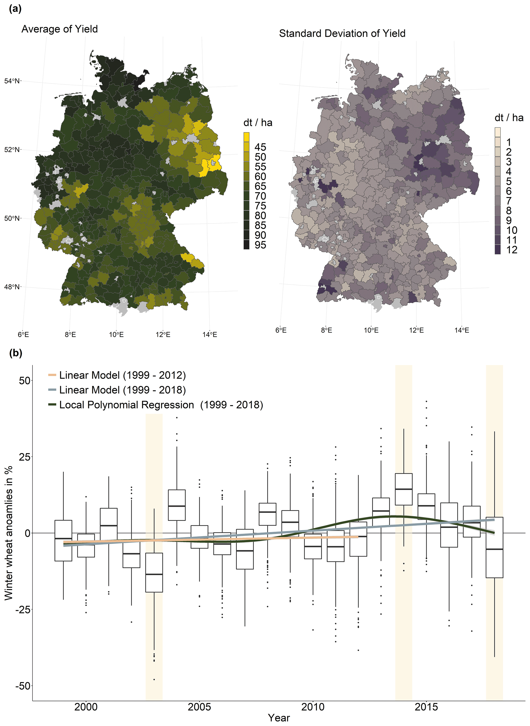
Figure 1 (a) Twenty-year winter wheat yield average (1999–2018, left) and standard deviation (right) of yields for the districts over Germany. (b) Box-and-whisker plots of winter wheat anomalies for each year and both linear and non-linear model fits to identify significant trends in the anomaly data. The exceptional years 2003, 2014, and 2018 are marked with a light beige box. Data source: Federal Statistical Office DESTATIS.

2 Data

The annual yield data for winter wheat are provided by the Federal Statistical Office for the districts from 1999 to 2018 (Statistisches Bundesamt (Destatis), 2019). Winter wheat has the largest share in cultivated area (2018: 46 %) and total production (2018: 51 % of quantity harvested) amongst all crops in Germany (Statistisches Bundesamt (Destatis), 2018). Figure 1a shows a map of the average yield and the standard deviation for the period 1999–2018. On average, the highest yields are recorded in the extreme north of Germany, while the lowest yields and the highest inter-annual variation are found in the eastern part of Germany. For each district, the data are converted into yield anomalies in percent by subtracting the average yield and dividing the resulting difference by this average. We have not corrected the yield data for the trend in order to take for example technological developments into account. Since the mid-1990s, annual yield increases have stopped, and no trend in yields has been observed since then (Gömann, 2018). This is shown in Fig. 1b, which shows the distribution of yield anomalies for the period 1999–2018. A positive linear trend can be observed for this time period (blue line). However, as can be seen from the green line, which represents the fit of the local polynomial regression, this positive linear trend is mainly associated with the above-average yields from 2013 onwards, which first rise rapidly and then fall again. Accordingly, almost no linear trend can be observed for the years before that (orange line in Fig. 1b). A trend correction is therefore not necessary. All districts with yield data of less than 10 years of observations are removed from the analysis, which results in 350 remaining districts (Fig. A1 in the Appendix shows a map of the numbers of observations available for each district).

Table 1 Table of the indicators of seven extreme weather conditions as well as an index for soil moisture for different soil depths. Column 2 shows the corresponding meteorological conditions and months of occurrence. The indicators (first column) are generated by counting the days above or below the thresholds of certain meteorological variables for specific months (second column). The variable names of the resulting features are displayed in the last column. The number indicates the month. For example, Frost10 represents the number of days with black frost in October of the previous year and Heat6 the number of days with heat in June. T reflects temperature, P precipitation. SMI denotes the soil moisture index for the uppermost 25 cm, SMIa for the entire soil column.

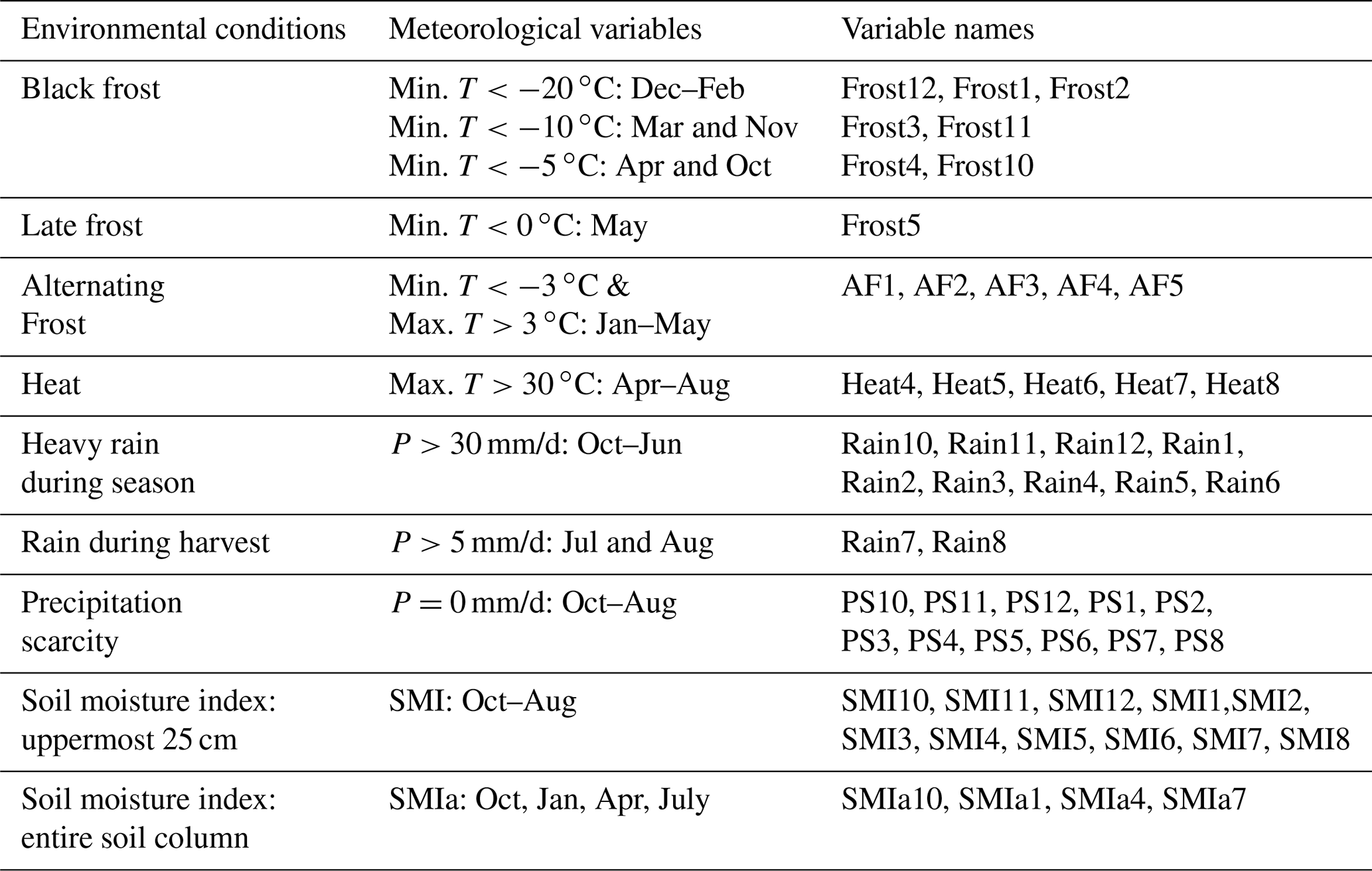
The daily temperature and precipitation data are obtained from a network of stations of the German Weather Service (Deutscher Wetterdienst, 2019). For the interpolation method to gridded data, see Zink et al. (2017). Daily meteorological data are converted to monthly aggregates by counting days above or below a defined threshold based on Gömann et al. (2015) and expert knowledge from farmer interviews. Table 1 shows the seven meteorological extreme indicators, the underlying meteorological and hydrological variables and considered months, as well as the corresponding variable names in the model.

The soil moisture simulation was obtained from the German Drought Monitor (Zink et al., 2016) using the mesoscale Hydrologic Model (mHM) (Samaniego et al., 2010; Kumar et al., 2013). In general, the model is grid-based with a spatial resolution of 4 km. Various hydrological processes such as infiltration, percolation, evapotranspiration, snow accumulation, groundwater recharge and storage, and runoff, both rapid and slow, are considered to calculate soil moisture. The model is driven by hourly or daily meteorological forcings (e.g. precipitation, temperature). For parameterization, it uses the spatial variability of observable but high-resolution physical properties of the catchment (land surface descriptors such as the digital elevation model, slope, aspect, rooting depth based on land cover classes or plant functional types, plant canopy characterization, soil texture, and geological formation type). The main feature here is the multiscale parameter regionalization, which is critical for achieving cross-scale flow matching. It allows the derivation of seamless parameter arrays between the targeted resolution and the high-resolution land surface descriptors (Samaniego et al., 2017). However, no endogenous land use management processes are considered. The depth of the soil in each grid cell depends on the soil type used in the mHM.

Soil moisture is presented here as an index because an index configuration supports the reduction of systematic errors of data that are simulated as well as spatially processed, such as in the present study (Auffhammer et al., 2013; Lobell, 2013). The soil moisture index (Samaniego et al., 2013) is derived from a non-parametric and site-specific cumulative distribution function of soil moisture for the period 1951–2019 for each month of the vegetation period of winter wheat. The percentile-based index thus quantifies the likelihood of occurrence of the monthly absolute soil moisture. The index ranges from 0 to 1 and represents an anomaly with respect to the monthly long-term soil water median (soil moisture index =0.5). Low values represent extremely dry soils and high values represent extremely wet soils. Consequently, seasonal effects due to drought and wet conditions during different agrophenological stages are taken into account. In this context, the interpretation of the monthly indices must take into account that the proportion of saturated soil changes over time and thus the base value for the index of each month. For Germany, this seasonality of soil moisture is shown in Fig. 4 in Samaniego et al. (2013). Here, we include two variables denoting soil moisture at two depths, namely the uppermost 25 cm (SMI) and the total soil column (SMIa) with variable depth depending on the soil map BUEK1000 (BGR, 2013). Soil moisture provides an integrated signal of meteorological conditions in the previous and subsequent months, which depends on determinants such as soil texture and depth, among other factors (e.g. Orth and Seneviratne, 2012; Samaniego et al., 2013). This long-term temporal persistence of soil moisture is relatively high compared to pure meteorological measures. It therefore does not allow for cumulative measures, such as those commonly used for temperature (e.g. growing or killing degree days, Schlenker and Roberts, 2009), but supports the use of monthly averages. Because of the high positive time correlation of soil moisture that accounts for the entire soil with its first- and second-order neighbours, only October, January, April, and July are considered for SMIa (Fig. A2, Appendix). In contrast, all months of the growing season are used for soil moisture of the upper 25 cm. The yield data are available for the districts of Germany. The meteorological data and soil moisture, which have a spatial resolution of 4 × 4 km², are thus aggregated to the districts. See Peichl et al. (2018) for a detailed description of the spatial processing (e.g. grid cells that are not non-irrigated agricultural land are excluded and the remaining cells are used to calculate the respective district average).

3 Method

We apply the machine-learning method random forests to explain the variation of winter wheat anomalies by the hydro-meteorological features introduced above. Random forests (RFs) have been used to analyze the effect of meteorological determinants on crop yields on a global scale (Jeong et al., 2016; Vogel et al., 2019) and in specific countries or regions (Jeong et al., 2016; Hoffman et al., 2018; Beillouin et al., 2020). However, none of these approaches explicitly used a measure of soil moisture, nor did they apply clustering to take into account the region-specific yield potential. RFs have also been widely used in related disciplines such as drought impact assessment (Bachmair et al., 2016) and forecasting (Sutanto et al., 2019). Within these applications, it has proven to be more powerful for classification than other data-science methods (Bachmair et al., 2017). Here, for a domain covering the whole of Germany, RFs proved to be superior to other machine-learning algorithms that are particularly suitable for non-linear systems, such as support vector machines and gradient boosting (not shown). This result is in alignment with other studies on a global scale (Vogel et al., 2019). A comparison of RFs to least absolute shrinkage and selection operator in the Northern Hemisphere proved comparable for a binary classification approach for simulated crop failures (Vogel et al., 2021). A RF randomly produces numerous independent trees as an ensemble to avoid over-fitting and sensitivity in the configuration of training data while being very efficient (Sutanto et al., 2019). The trained model is Breiman's RF (Breiman, 2001a). It is tuned to the number of variables available for splitting at each tree node (parameter mtry) using the tuneRF function of the R package randomForest (Liaw and Wiener, 2002). The initial values of the parameters are set to default, the number of trained trees is 500, and the tuning is based on an out-of-bag error estimation (see e.g. James et al., 2013, for more information).

The crop yield potential varies regionally in Germany due to differences in climate and soils, among other factors. To take account of these differences, a spatial clustering was implemented to identify different sub-regions within Germany. The clustering methods used are representatives of centroid-based ones, such as k-means (KMEANS, MacQueen, 1967; Hartigan and Wong, 1979) and partitioning around medoids (PAM, Kaufman and Rousseeuw, 1990), which is less sensitive to outliers, as well as the connectivity-based hierarchical clustering (HIERARCHICAL, Murtagh, 1985). Standard internal validation such as connectivity, average silhouette width, and Dunn index for cluster numbers between 2 and 16 were tested for the evaluation. However, the results show no clear outcome on which algorithm and size combination to use (Fig. A3). Instead, we fit the random forests individually for each region defined by one of the cluster algorithms and cluster sizes. We then selected the combination that maximizes the average prediction capacity (test R-squared – R²) across all regions. For each of these cluster configurations the model is trained on 80 % of the data in that subset (randomly selected from all space and time combinations) and predicted for the rest. For this approach, the cluster sizes were limited, so that each cluster contains at least 300 data points and the cluster sizes are the same for all three algorithms. The respective maximum cluster size is thus 9. The data used for clustering are monthly averages and daily observations of the meteorological data for the entire year. Soil moisture index is included for both the upper layer and the entire soil column. Average yields are also taken into account in the data for cluster formation. This is based on the intuition of taking into account time-invariant factors of each cluster that affect yields such as soil quality and average farm size. These factors are not considered in the random forest due to the use of yield anomalies. This approach is inspired by fixed-effect econometric models. There, the group means are fixed, thus taking into account the time-invariant heterogeneity of these groups (for the econometric literature, see for instance Wooldridge, 2012).

The random forest algorithm allows us to study the relationships between hydro-meteorological extremes and yield anomalies by assessing the relative importance of the variables and the functional relationship between each predictor and the response variable (Jeong et al., 2016; Vogel et al., 2019; Beillouin et al., 2020). For the latter, we use model agnostics, which include various flexible methods that allow the interpretation of black box models that separate the explanation of the model from the model itself. Accordingly, the same method can be used for any kind of machine-learning algorithm, and different types of explanations and different types of features can be presented (Ribeiro et al., 2016). The particular method considered here is accumulated local effects (ALE), which is a visualization of the average marginal effect of features on target variables for supervised learning models (Apley and Zhu, 2016; Molnar, 2020). ALE plots predict the effect of an explanatory variable across their realizations, taking into account only a subset of the sample with observed values adjacent to the respective realization (Apley and Zhu, 2016). It is a faster alternative to the popular approach of the partial dependence plots (Friedman, 2001), which have already proven to be suitable in the context of yield prediction (Jeong et al., 2016; Vogel et al., 2019). However, ALE plots are more suitable for visualizing marginal effects by plotting explanatory variables against the predicted outcomes if the features are highly correlated (Storm et al., 2020; Molnar, 2020). One limitation is that uncertainty estimates are not provided for ALE plots, which is a substantial limitation of the approach and is an area of active research (Storm et al., 2020; Molnar et al., 2020). The ALE plots are shown for the most important features of each cluster.

Table 2 Table with the average R² for the test and training samples for the three best combinations of cluster algorithm and cluster size (in parentheses) for three soil moisture configurations.

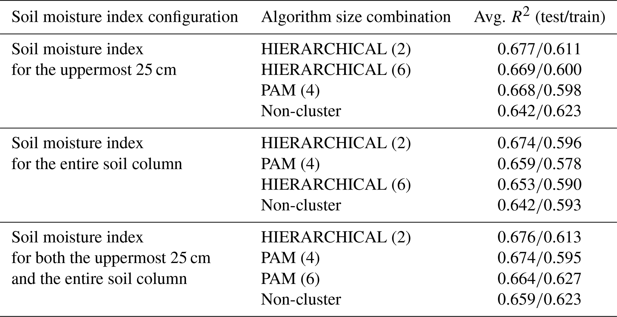
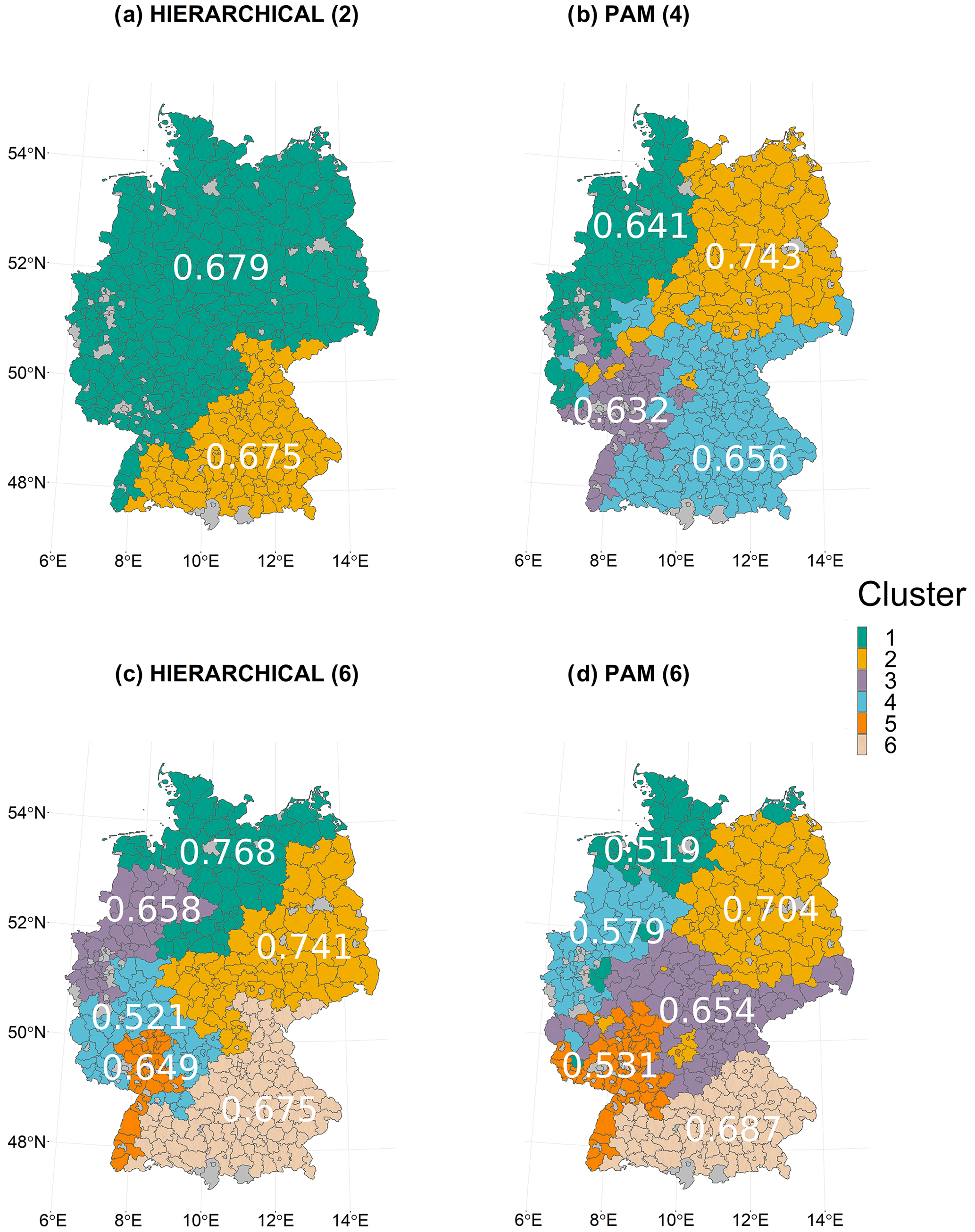
Figure 2 Spatial structure of clusters shown in Table 2. The clusters are derived from the HIERARCHICAL cluster algorithm with cluster sizes (a) 2 and (c) 6 and from the PAM algorithm with cluster sizes (b) 4 and (d) 6. The white numbers indicate the respective test R² for each cluster derived considering only the top 25 cm soil layer (a, b, c) and for (d) with both the top and the entire soil column, since PAM (6) is relevant only for this configuration.

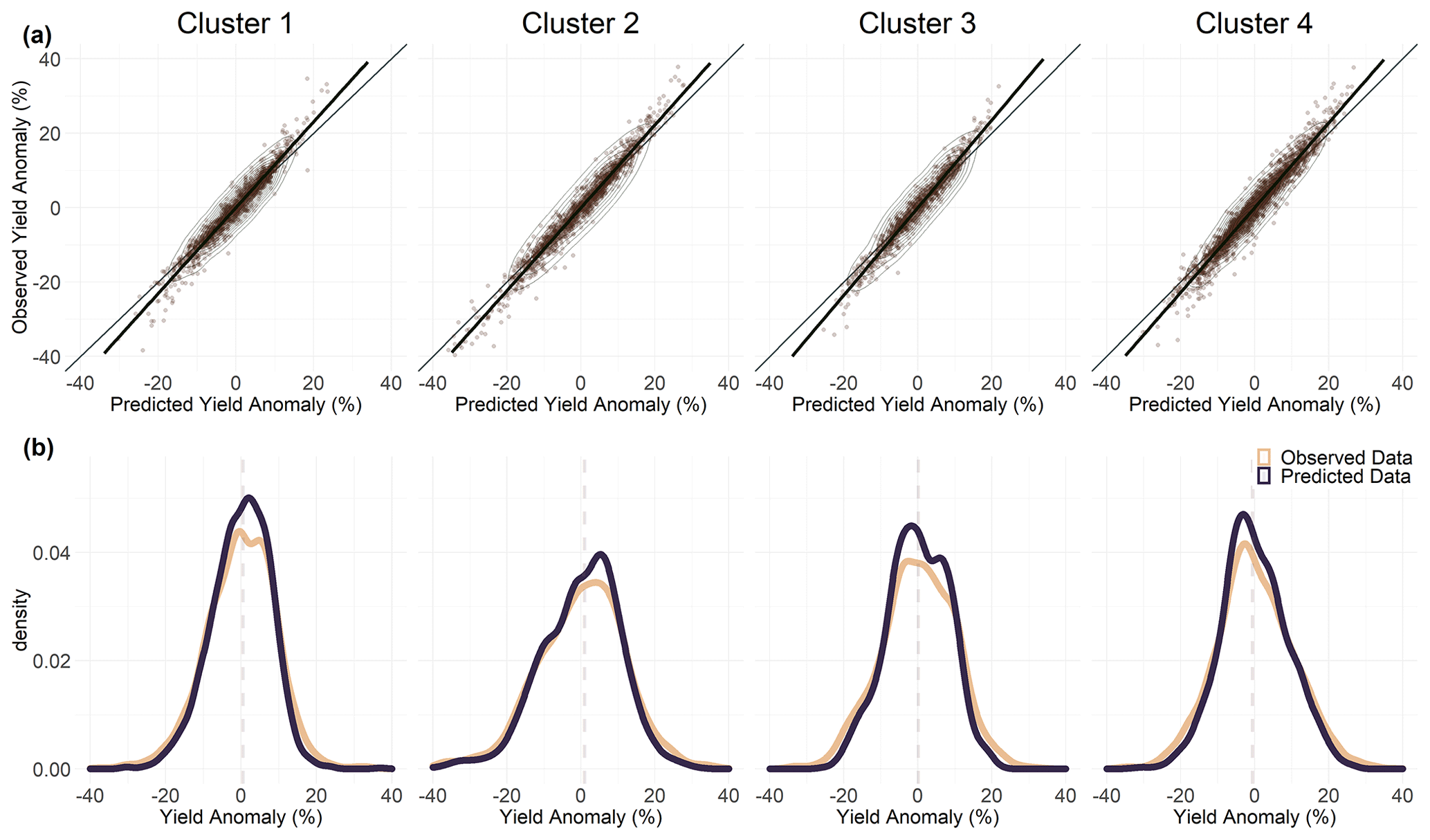
Figure 3 Scatter (a) and density (b) plots of the observed and predicted data for the four clusters derived using the PAM algorithm with size 4. The bold black lines in the scatterplots indicate the linear regression line and the ellipses represent the contours of a 2-D density estimate of the points.

4 Results

4.1 Evaluation of spatial clustering

To evaluate the cluster algorithm and the number of clusters, the test R² is created using the RFs for each combination of the clusters and the sizes of the clusters. Table 2 shows results for three different soil moisture configurations, i.e. one each for the upper layer as well as the entire soil column and one that takes both into account. For each of these soil moisture configurations, the three combinations of algorithms and cluster sizes with the highest test R² are shown. The R² derived from the training data is also shown. In general, the test values are higher compared to those derived from the training sample. This generally indicates good out-of-sample predictive ability of the model. In this context, the sample is based on randomly selected combinations of years and administrative districts. Furthermore, all the configurations presented have very similar predictive capacities. Overall, the best results can be achieved if only a soil moisture index for the uppermost 25 cm is considered. Since the data for the entire soil column do not appear to provide any additional information for the model, we rely only on the top 25 cm for further analysis. The best results explain 68 % of the wheat yield anomaly variation. The average variance explained exceeds the variance explained by RFs applied at the global level (Vogel et al., 2019) or for the Northern Hemisphere (Vogel et al., 2021) and is comparable to the highest explained variability for RFs applied to European regions, with an average for winter wheat of 43 % (Beillouin et al., 2020). A comparable regression model approach is able to explain a maximum of 32 % of the variation (Gömann et al., 2015). A large fraction of the variability is usually explained by time-invariant factors, which are largely not considered here due to the demeaned yield data. For example, Peichl et al. (2018), using a regression model for silage maize, showed that up to 32 % of the variation explained by the model is explained by time-invariant factors. An approach modelling relative year-to-year yield changes has similar results (Conradt et al., 2016). There, the best explanatory power is found for northern and eastern Germany, with comparable coefficients of determination. However, for the rest of Germany the model presented here performs better as it is doing well in regions with rather low yield variability such as in the south of Germany (cluster 4 in Fig. 2b and cluster 6 in Fig. 2c and d). We decided to further investigate the results of PAM using four clusters that offer a compromise between the highest possible predictive power and sufficient complexity to adequately represent relevant mechanisms. Here, cluster 1 mainly represents the north-western and very western parts of Germany, cluster 2 the north-east, cluster 3 the extreme south-west along the Rhine, and cluster 4 most parts of central and southern Germany (Fig. 2b). The test R² of cluster 2 is the highest at 0.743, followed by clusters 4 (0.656), 1 (0.641), and 3 (0.632). For all four clusters, a good fit can be observed in the scatterplots for most of the data (Fig. 3a), while the tails are slightly underestimated (Fig. 3b). The higher explanatory power for cluster 2 might be related to the higher variation in yield anomaly there (see Fig. 1). In addition, different impact mechanisms operate within each cluster, which are decomposed in the following.

4.2 Marginal effects of the most important features

The main variables for each sub-cluster and the corresponding average marginal effects are presented below in order to understand the range of adverse effects on yield variation in winter wheat. To generate variable importance and ALE plots, no split is made between test and training data. The non-cluster results are compared with the spatial clusters generated with the PAM clustering algorithm for a cluster size of 4 – PAM (4). The detailed ALE plots for the overall best algorithm cluster size combination, i.e. the HIERARCHICAL cluster algorithm with two clusters considering only the top 25 cm of the soil column, are provided in the Appendix (Fig. A5). In addition, the ALE plots for the HIERARCHICAL (6) (Fig. A6), which consider only the top 25 cm for the soil layers, and those of the three best-ranked cluster algorithm and size combinations of both soil moisture for the top 25 cm and the entire soil column, are shown (Figs. A7, A8, A9). The feature effects shown here can be interpreted as additive because they are purged of correlation with other features. For example, the combined effect of soil moisture in June and July is the sum of SMI6 and SMI7.

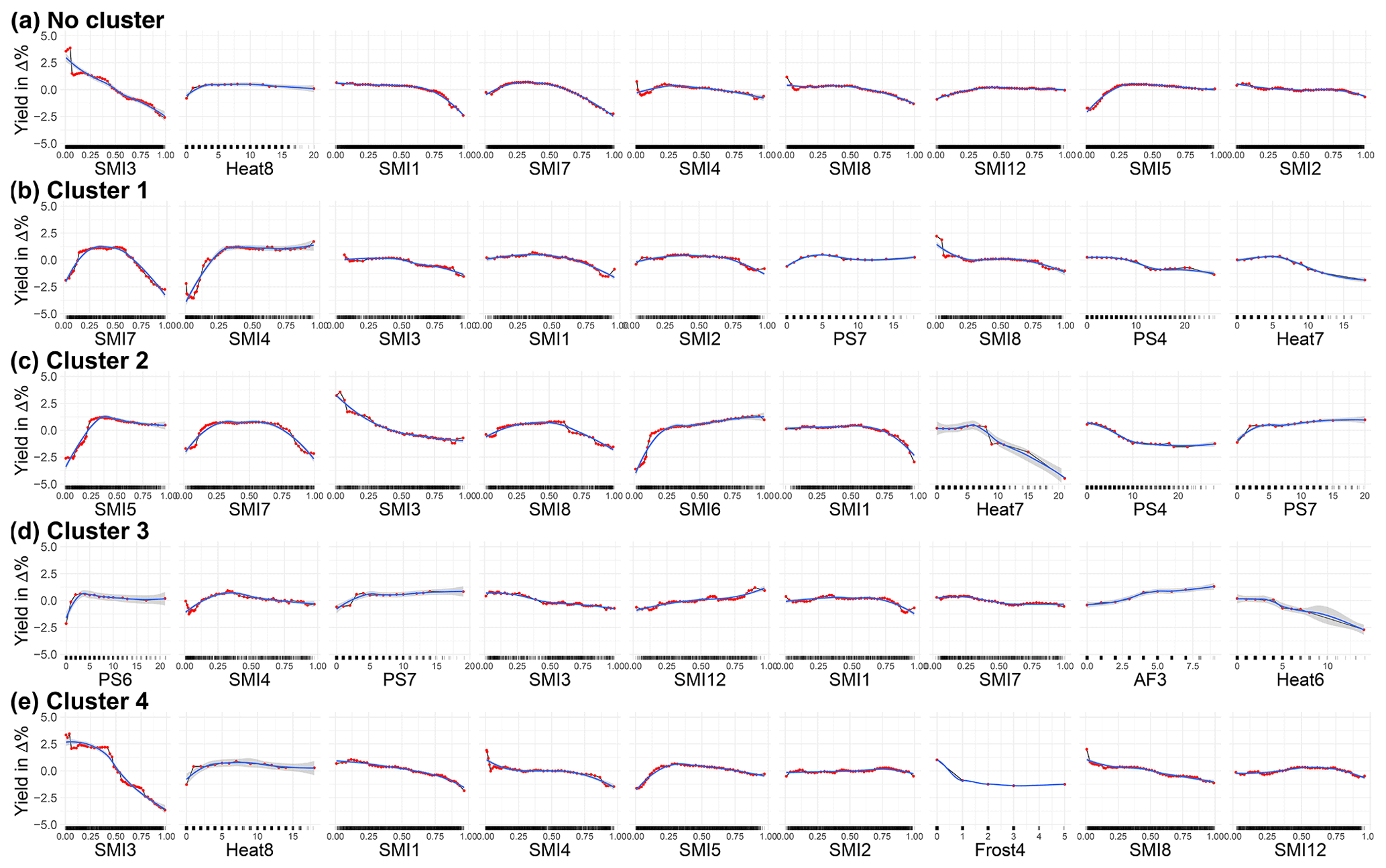
Figure 4 Accumulated local effects plots of the nine most important features for no cluster (a), cluster 1 (b), cluster 2 (c), cluster 3 (d), and cluster 4 (e) derived from PAM (4). The red dots are estimated by the ALE plot algorithm (FeatureEffects of the iml package in R). We have chosen a grid size of 50, which allows us to reveal the true complexity of the model at the expense of shakiness. Therefore a non-linear smoothing function (LOESS – locally estimated scatterplot smoothing) is added in blue (with the confidence interval in grey). SMI represents the soil moisture index for the uppermost 25 cm of the soil column, PS stands for days without rain in a given month, Heat stands for days with a maximum temperature of more than 30 ^∘C, Frost stands for the number of days below −5 ^∘C (as only April is indicated), and AF stands for days with a minimum temperature below −3 ^∘C as well as a maximum temperature of $+{\mathrm{3}}^{\circ }$C (same day). The number indicates the month; 10, 11, and 12 refer to the year before. For example, SMI12 represents SMI in December.

The ALE plots in Fig. 4 are ranked in accordance with their variable importance (for further information, see the variable importance section in the Appendix). In general, soil moisture supports best the performance of the model. In both the non-cluster approach and clusters 1 through 4, at least 7 of the 12 most important features are derived from soil moisture (Fig. A4). Cluster 3 relies the least on soil moisture, while in cluster 4 the most is explained by soil moisture.

Figure 4a shows the ALE plots for the non-cluster approach. The three main effects shown for the whole country are the same as in cluster 4, i.e. soil moisture in March (SMI3), heat in August (Heat8), and soil moisture in January (SMI1). The functionality found in both non-cluster as well as cluster 4 is very similar in this regard. SMI7, the fourth-ranked feature, is very important in both cluster 1 (1st) and cluster 2 (2nd), and the functionality is a combination of both. SMI4 (5th in non-cluster) is found with similar crop responsiveness in cluster 3 (2nd) and SMI8 (6th in non-cluster) in cluster 1 and cluster 4. For the three last-ranked features, the sensitivity of SMI12 looks like a combination of those found in clusters 3 and 4, SMI5 of clusters 2 and 4, and SMI2 of clusters 1 and 4. For the non-cluster approach, more water in the top 25 cm of soil is more harmful than beneficial to plant growth in most months. The notable exceptions here are May (SMI5) and, to some extent, July (SMI7). Overall, the sensitivities for the non-cluster approach are not very pronounced, which could come from the fact that it shows combined effects of areas with different plant susceptibilities due to different environmental conditions as well as possible interactions with other variables. The largest effect is shown for soil moisture in March (SMI3).

For cluster 1 (Fig. 4b), the greatest plant sensitivities to environmental conditions for the SMI are found in July and April. While extremes at both ends are detrimental for July (SMI7), this is mostly the case for drier-than-normal conditions in April (SMI4). In addition, each day without precipitation in April reduces yield (PS4). Furthermore, heat is beneficial up to 6 d in July but has a negative effect above this threshold. In the first quarter of the year (SMI1, SMI2, SMI3) as well as in August (SMI8), higher SMI values may be more associated with negative impacts on crop yields. Cluster 2 (Fig. 4c) corresponds to the area for which the modelling approach also has the highest explanatory and predictive power (Table 2). The sensitivities shown there are also the largest. A drought signal can be found in particular for May (SMI5) and June (SMI6) and to some extent for July (SMI7) and August (SMI8). In March (SMI3), drier-than-normal conditions are preferred. In January (SMI1), July (SMI7), and August (SMI8), wetter-than-normal conditions are detrimental. In general, for the SMI features, a pivotal transition in the patterns takes place between April and May, as the negative effects of drought are evident first in May. Heat plays an even more critical role in July than in cluster 1 (Heat7), but the uncertainty in the LOESS function is also larger due to the small number of realizations. In addition, additional days without rain are adverse in April (PS4) but favourable in July (PS7). The cluster for which meteorology plays the most decisive role is number 3 (Fig. 4d). In June and July, too few rain-free days have a negative impact on winter wheat yield (PS6 and PS7). Overall, drier conditions are preferred in July (PS7 and SMI7) but also in March (SMI3), while the opposite is true in December (SMI12). On the other hand, excessively wet soil moisture conditions are harmful in the following month (SMI1). A low drought signal based on soil moisture is noted for April (SMI4). More than 4 heat days in June (Heat6) become increasingly detrimental with each additional day above 30 ^∘C. This feature has the greatest potential for damage, but the extreme impacts are also associated with high uncertainty. The cluster is the only one that also represents alternate frost, here for March (AF3). Cluster 4 (Fig. 4e) is largely dominated by soil moisture, of which January (SMI1), April (SMI4), and August (SMI8) show a slightly negative correlation with crop yield, and for March (SMI3) it is strongly negative. May shows a drought signal up to an index of about 0.3 (SMI5) and is then also negatively correlated. For February (SMI2) and December (SMI12), only a small effect of soil moisture on crop yield can be detected. The second most important variable is heat in August (Heat8), with at least 1 d of up to 10 heat days being beneficial. Late frost in April (Frost4) is an important and detrimental meteorological determinant.

Previous studies showed that water deficit has no limiting effect on wheat yield in North Rhine-Westphalia (Kropp et al., 2009) or showed a higher sensitivity of wheat yields to water surplus compared to drought for Germany as a whole (Zampieri et al., 2017). Similar observations can be made for the non-cluster approach as well as for most clusters defined by PAM (4). For many regions in Germany for most growing stages, extensive wet periods with water-saturated soil represent an extreme weather situation for agriculture (Gömann, 2018). In our study, soil moisture in March is the most important variable (see Fig. A4). It dominates both the non-cluster setting and cluster 4 and is at least fourth in the other clusters. The relationship between the SMI and yield anomalies is negative (in varying sensitivities) for the entire range of the SMI in March. This indicates that yield losses are associated with higher-than-normal water content in the upper 25 cm of soil. The most sensitive growth phase for waterlogging is after germination but before emergence (Barber et al., 2017; Grotjahn, 2021). Oxygen deficiency can cause damage to the plant that results in yield losses (Cannell et al., 1980). In addition, excessive soil water fosters pathogens (Grotjahn, 2021) and complicates plant treatment operations (Urban et al., 2015; Gömann, 2018). This finding is consistent with the results of Ben-Ari et al. (2018), which showed that a combination of abnormally wet conditions in spring together with abnormally warm temperatures (not controlled for in this study) in late autumn led to large losses in winter wheat in France in 2016. An evaluation of the interaction effects to treat possible compounding events does not show stable results and varies from run to run, probably due to the lack of available data. Therefore these results are not discussed here but need to be evaluated in further studies.

A strong drought signal can only be found in the data if the model is applied to a sub-region such as cluster 2 (Fig. 4c). In a non-cluster approach, those signals are mostly confused. This underlines the importance of using clustering to take account of different crop yield potentials and environmental conditions. In cluster 2, for the months of May through July, dry conditions below a certain threshold are more damaging than too much water in the soil. The crop can tolerate (May and June) or even benefit from (July) drier-than-normal conditions during this period until soil water content is lower than about the 25th percentile of the empirical distribution of soil water content in the top 25 cm of soil. At levels below this threshold, the effect on crop yield is negative. Expected wheat yields (relative to 0 in ALE plots) decrease by about 4 % in June and 2.5 % in July, when the SMI is less than about 0.125 and about 2.5 % when the SMI is less than just below 0.25 in May. Yield losses are even more when compared to the entire potential of SMI impacts of the respective months. For example, in July, the largest difference between yields is 5 % when comparing an SMI value close to 0 and close to 1. Thus, these values define critical relative thresholds. The observation that the absence of water governs crop production in eastern Germany is in alignment with recent studies (Conradt et al., 2016; Vinet and Zhedanov, 2010). There, lack of precipitation together with sandy soils, which have a lower water holding capacity, may result in water shortage for winter wheat growth (Rezaei et al., 2018). According to phenological evidence, this strong negative water deficiency signal makes sense because it is associated with the drought-sensitive vegetative and generative phases of winter wheat (Lüttger and Feike, 2018).

In general, it is difficult to disentangle the compounding effects of heat and water supply on plant growth (Gourdji et al., 2013; Roberts et al., 2013; Lobell and Asseng, 2017; Roberts et al., 2017; Schauberger et al., 2017; Siebert et al., 2017; Zscheischler and Seneviratne, 2017; Mäkinen et al., 2018; Peichl et al., 2018). Previous studies show that the specific contributions of temperature and precipitation anomalies to drought are difficult to isolate (Zscheischler and Seneviratne, 2017; Vogel et al., 2019). Moreover, the negative yield effects of high temperatures are associated with water stress and can be mitigated by irrigation (Frieler et al., 2017; Vogel et al., 2019; Ribeiro et al., 2020). However, for Germany, studies show that heat has historically been more damaging than drought at sensitive growth stages (Lüttger and Feike, 2018; Trnka et al., 2014). Vogel et al. (2019) showed on a global scale with a very similar approach that temperature-related indicators such as frequency of warm days, growing season average temperature, and average daily temperature have the highest predictive power for crop yields. Here, a heat signal is observed in June for cluster 3 and in July for cluster 1 and with higher sensitivity for cluster 2, which could be related to the most heat-sensitive phase of anthesis (Barber et al., 2017; Rezaei et al., 2018). These signals cannot be detected in the non-cluster approach as well as when considering only clusters of size 2 as in Fig. A5 and Fig. A7. In clusters 1 and 2, more than 6 and 8 heat days above 30 ^∘C in July, respectively, show adverse effects, a period that could be related to grain filling (Lobell et al., 2012; Lüttger and Feike, 2018; Mäkinen et al., 2018). In cluster 4, heat in August, a period generally associated with ripening, has positive effects for each additional day and negative effects after the seventh day. Our approach, which explicitly controls for plant water supply through soil moisture, shows, however, more negative effects related to water deficit compared to heat for the non-cluster approach as well as for cluster 1 and cluster 4. In cluster 2, July heat has the largest negative effect in amplitude found in this study (albeit with large uncertainty). However, each month from May through August exhibits drought-related impacts that are greater in total than the heat-related impacts. In cluster 3, meanwhile, the heat in June has a greater impact than the lack of precipitation in the same month and the lack of soil moisture in April combined. This underscores the importance of disentangling environmental factors in plant development in terms of temporal and spatial occurrence, as this has critical and significant implications for management and adaptation actions.

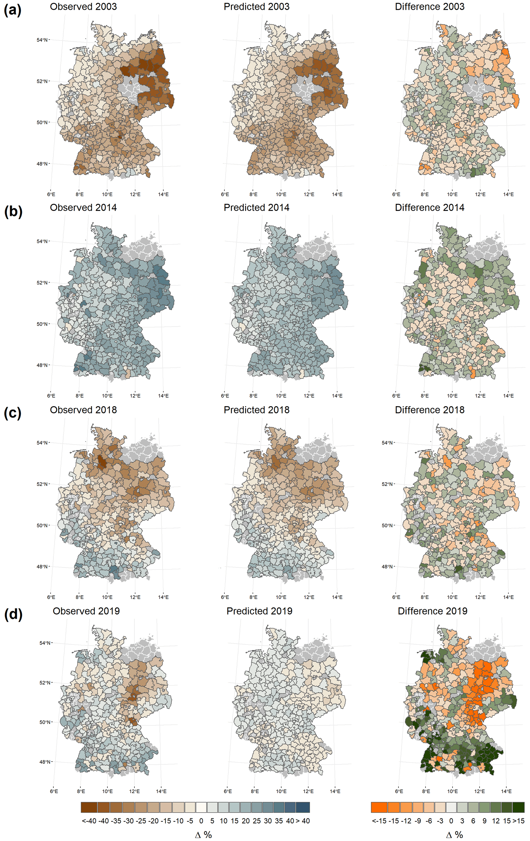
Figure 5 Maps of the observed, the predicted (for PAM clustering with four sub-regions), and the difference between these two for winter wheat yield anomalies for the in-sample years 2003 (a), 2014 (b), and 2018 (c) as well as 2019 (d), for which the model was not trained, at the district level. Administrative districts with missing data are displayed in grey.

4.3 Predictions of years with extreme yield anomalies

Figure 5 shows the maps of observed, predicted, and the difference between those two for winter wheat yield anomalies for the in-sample years 2003, 2014, and 2018 as well as for 2019. The latter year is not included in the training period 1999–2018 to allow the assessment of the out-of-sample predictive skill of the model. The first three are the years with both the largest losses and gains during the training period. Those years show different spatial patterns in yield gains and losses. In 2003, the year with the highest total volume of losses, the largest losses were recorded in eastern Germany. For the year 2018 the losses are more likely to be in the northernmost parts of Germany, while the south of Germany shows positive yield anomalies; 2014 is a particularly good year with higher than expected yields, especially in the easternmost parts of Germany. The general spatial patterns of losses and gains of the observed data are reproduced by the simulated data for all 3 years. However, as can be seen from the differences, the model tends to slightly underestimate the extent of both extremes. For example, the largest negative differences between observed and projected data for 2003 are found for Vorpommern-Greifswald, a district in the north-east of Germany. The region around this district also shows the largest contiguous area of negative differences, i.e. an underestimation of the losses. The largest positive difference is found in the very south. For 2018 the picture is comparable and the positive yield anomalies in the south and the negative anomalies in the north are underestimated. However, for both years, there is no clear pattern of overestimation and underestimation of non-extreme values. For 2014, the very positive results in some of the eastern districts are underestimated. However, the highest positive differences are not consistent with the highest positive anomalies observed. The highest differences in the positive anomalies are those for the high yield anomalies in the extreme south-west. The highest negative differences are those for the underestimated losses in southern Bavaria. For the in-sample years 2003, 2014, and 2018 the model is very well able to predict district yield anomalies but does not represent the full extent of the anomaly variation in the extremes. With less variation in the observed yield data, no clear pattern of underestimation or overestimation can be observed. A different picture can be observed for the out-of-sample year 2019. There, both losses and gains are structurally underestimated and the full range of variation of the observed yield anomalies is not represented in the predicted yield anomalies. This shows potential difficulties of out-of-sample predictions of machine-learning models such as random forest. With sufficiently large tree size, the out-of-bag estimator used in this study converges with estimates based on leave-one-out cross-validation, which may promote overfitting compared to other cross-validation techniques (James et al., 2013). However, this is not indicated when comparing the test and training R² results in Table 2. Another possible reason is that out-of-sample structural relationships and functional relationships of a given year are not detected or adequately reflected by this approach. For one, corresponding patterns affecting wheat yields in 2019 might not have occurred in the 1998–2018 training period. On the other hand, loss events due to certain determinants, compounded or isolated, could have occurred in 2019, which may not have been appropriately detected by the model or may not have been extrapolated from the sample by the model to a sufficient degree.

5 Conclusions

Here we show that random forests are very suitable for assessing the non-linear damaging effects of different environmental conditions on winter wheat yield anomalies. Explicit consideration is given to soil moisture at various depths. In addition, the crop yield potential and other spatially related environmental conditions are taken into account, which helps to improve predictive power. Different clustering algorithms and cluster sizes have been applied to improve the predictive capacity of the model from 64 % in average test R² to 68 % when only considering the uppermost 25 cm in the soil column. In general, the approach is able to explain the general pattern of losses and gains of the districts, also those in particularly extreme years such as the years 2003, 2014, and 2018. In comparison to other models, this approach performs better in regions with low crop yield variation. However, it slightly underestimates the extremes, with this problem being more pronounced for out-of-sample predictions. This suggests that the out-of-sample predictive capacity of machine-learning algorithms such as random forest needs to be further explored both for use as a seasonal forecasting tool and in the context of climate impact assessment. Nevertheless, the analysis presented here can support the design of tailor-made and, above all, prompt support mechanisms for large losses caused by extremes as it helps to disentangle the damage spectrum for sub-regions as well as sub-seasonal effects in Germany. It particularly shows that soil moisture dominates the variable importance ranking. All over Germany, soil moisture abundance in March thereby ranks first and shows substantial negative effects. In addition, the abundance of water is problematic for the growth of winter wheat in most other parts of Germany. Water shortage signals can be found for all four clusters represented here; however, the most susceptible area is represented by cluster 2 (roughly the north-east of Germany). These water scarcity effects tend to go unrecognized in a non-cluster approach. The same applies to meteorological variables, such as heat-related measures in cluster 2 in July. Overall, these have a comparatively minor role in explaining the effects on yield anomalies in winter wheat but can still have a major impact on crop development. Again, this is especially the case in cluster 2, where heat in July has the greatest overall damage potential. However, across the season, more can be associated with drought-related measures based on soil moisture than heat. For example, 4 months of drought signal occur in the north-eastern cluster, while heat is only relevant in July. This information is helpful for tailoring management and adaptation measures. For example, it is particularly suitable for the insurance industry for providing index-based insurance policies, as they help to identify harmful features and visualize thresholds in those features that cause damage (Albers et al., 2017). Prominent examples of this are the large yield declines associated with an SMI smaller than 0.25 in May and 0.125 in June and July in eastern Germany. These sub-seasonal thresholds may also help to better determine drought classes for specific crops used in monitoring and decision support tools such as the German Drought Monitor. Furthermore, such an approach, which explicitly captures the complexity of the underlying reaction mechanism rather than relying on one major determinant, generally appears to be more suitable for the projection of climate impacts, since global climate models explicitly capture the dynamics of several hydro-meteorological variables (Crane-Droesch, 2018). However, further research is needed to better take into account small-scale events such as hail and thunderstorms and to better reflect region-specific differences in growth periods. The compounding effects of interacting characteristics also need to be studied in more detail and should be clarified using appropriate methods. In addition, it is important for seasonal forecasting to improve the ability to predict events outside the sample. Here, an extended time period for training the data might help. Furthermore, different cross-validation techniques might support the reduction of the variability in the predictions. Also, the use of other machine-learning algorithms or deep learning could help to further improve predictive capabilities by better capturing (annual) patterns not covered by this approach. Similarly, a sensitivity analysis of the expert thresholds used to define the extreme values could help to improve the model.

Appendix A

The Appendix contains additional information on the data, approaches to cluster validation, as well as plots of variable importance and accumulated local effects for the best combinations of cluster algorithm, cluster size, and SMI for a defined soil depth (either the top 25 cm or both the top 25 cm and the total soil column) that are not presented in the main text. Those are for the uppermost 25 cm soil moisture index configurations HIERARCHICAL (2) and HIERARCHICAL (6) and for the combination of the top 25 cm and total soil column HIERARCHICAL (2), PAM (4), and PAM (6).

A1 Map of available yield observations for each district

We use a spatiotemporal data set that includes 412 districts and 20 years. All districts with less than 12 years of reported yields (green areas) are excluded from the analysis (Fig. A1). The grey areas in the south are four districts for which non-irrigated agricultural land could not be identified. A total of 350 districts remained. Because of missing values, especially for Saxony-Anhalt and Mecklenburg-Western Pomerania and some parts in western Germany, the time series for these districts can be shorter than 20 years.

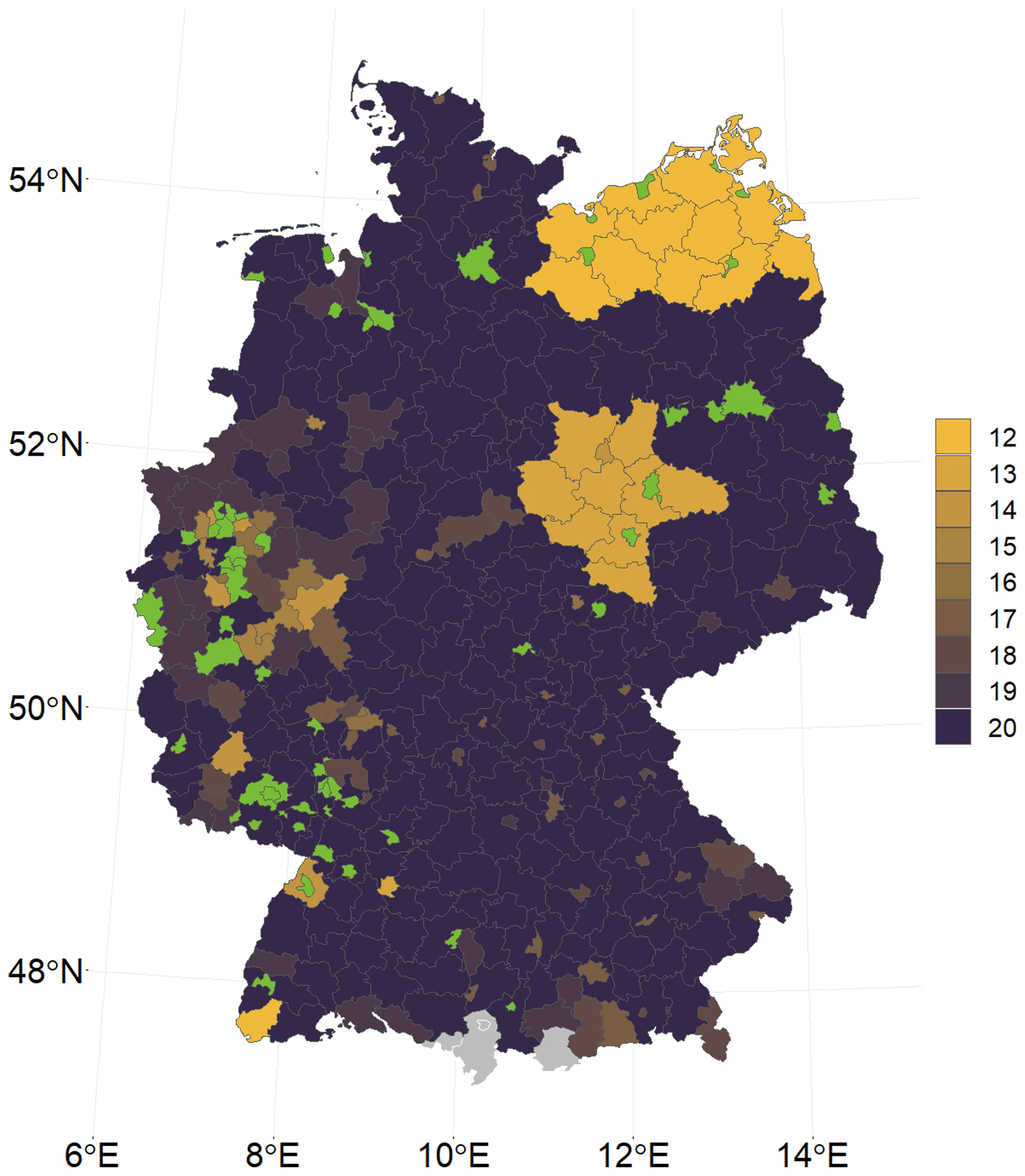
Figure A1 Map showing the number of available winter wheat yield observations for each district used in the analysis for the period 1999–2018. Green districts were removed because 8 or more years of winter wheat data were not reported by regional statistics. Grey areas are districts with no non-irrigated agricultural land.

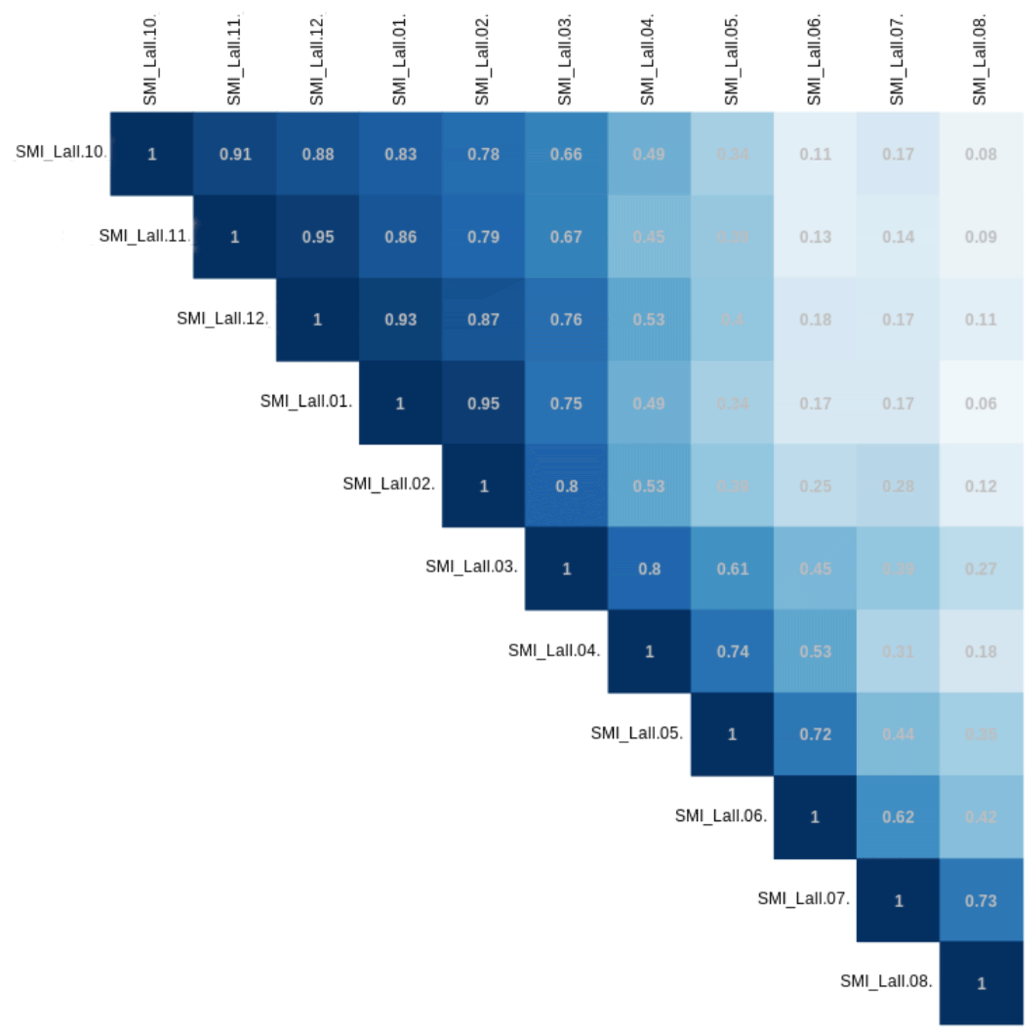
Figure A2 Correlation plot (Pearson correlation coefficient) of the soil moisture index for the entire root zone (Lall) for all months of the season of winter wheat. The SMI variables of October to December (10–12) refer to the previous year, since winter wheat is usually planted in late autumn and harvested in the summer of the following year.

A2 Correlation plot of the soil moisture index for the entire root zone for all months of the season of winter wheat

Figure A2 shows the correlation of soil moisture indices for total root zone depth for the season of winter wheat in Germany from October to August. This correlation shows the persistence of soil moisture and the smoother distribution resulting from it compared to meteorological variables. The Pearson correlation coefficient between the neighbouring SMIa is between 0.62 and 0.95. For the second-order neighbours it is still between 0.42 and 0.88. In general, the largest correlation coefficients are found for the first half of the season. For this reason, within the random forests, we consider only the months of October, January, April, and July.

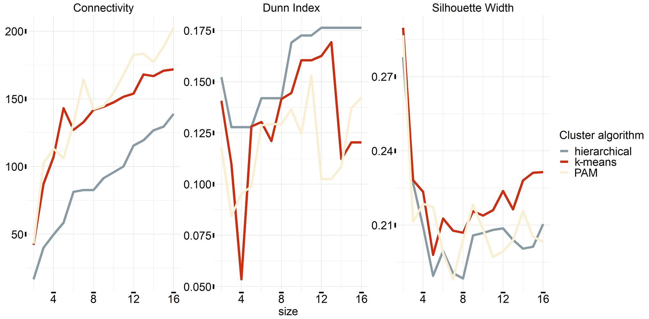
Figure A3 Internal validation measures for clusters with different sizes between 2 and 16. The measures depicted are connectivity, Dunn index, and silhouette width.

A3 Cluster validation

Here, we use internal validation measures to assess the quality of the clustering, which employ only the data set and the clustering partition for the assessment (Brock et al., 2008). The specified measures are connectivity, silhouette width, and Dunn index (see Fig. A3). Connectivity refers to the degree of connectivity of the clusters (Handl et al., 2005). It has a value between 0 and infinity and should be minimized. Both the silhouette width and the Dunn index represent linear combinations of compactness and separation of the clusters. The Dunn index has a value between 0 and infinity and should be maximized (Dunn, 1974). The silhouette width ranges between −1 and 1, and well-clustered observations have a value close to 1 (Rousseeuw, 1987). The connectivity mainly indicates the use of a small number of clusters, Dunn, at the other end, a rather large number. Silhouette width, by contrast, prefers a rather small number of clusters. Both connectivity and Dunn index mostly favour the HIERARCHICAL algorithm, while silhouette width prefers KMEANS. As a consequence of this ambiguity, we decided to evaluate the cluster algorithm and the number of clusters by the R² outside the sample, which is generated for each cluster and the number of cluster combinations for the separate soil moisture configuration.

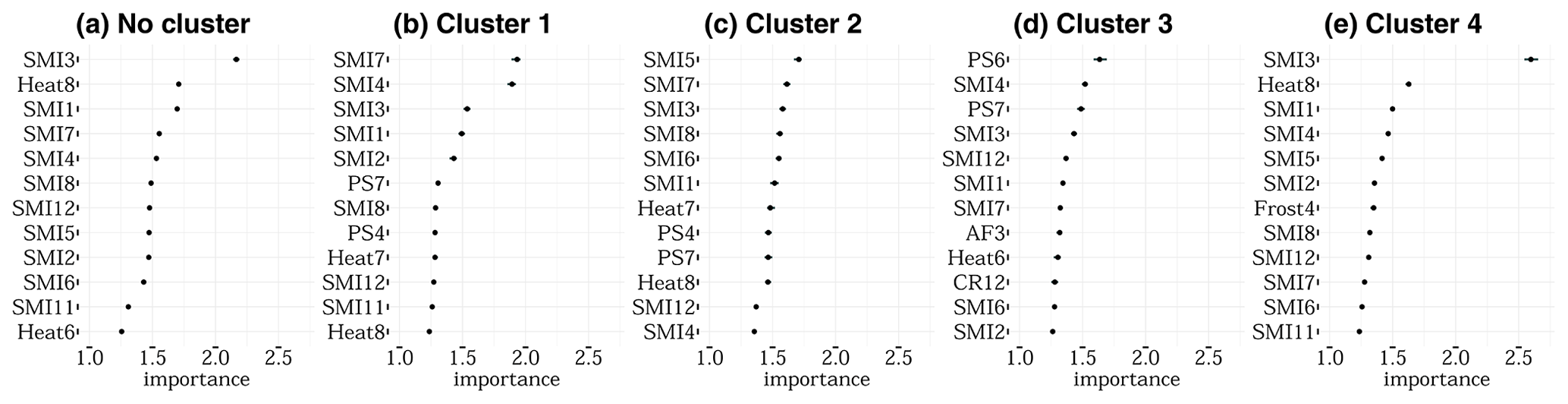
Figure A4 Variable importance of the 12 most important features for no cluster (a), cluster 1 (b), cluster 2 (c), cluster 3 (d), and cluster 4 (e) derived with the PAM (4) cluster algorithm and size combination only considering the uppermost 25 cm of the soil column. The importance ranking is established with 50 repetitions of permutation. SMI represents the soil moisture index for the uppermost 25 cm of the soil column, PS stands for days without rain in a given month, Heat stands for days with a maximum temperature of more than 30 ^∘C, Frost stands for the number of days below −5 ^∘C (as only April is indicated), and AF stands for days with a minimum temperature below −3 ^∘C as well as a maximum temperature of +3 ^∘C (same day). The number indicates the month; 10, 11, and 12 refer to the year before. For example, Frost10 represents black frost in October.

A4 Variable importance plots

Here, importance is defined as the factor by which the model's mean absolute error (mae), a measure of model performance, changes when the feature is shuffled (Molnar, 2020). To overcome the randomness added by this shuffling, the permutation is repeated 50 times and the results are averaged. Thus, the results show variability, indicated by the black bar, but rather small (Fig. A4). As Fig. A4a shows for a non-cluster approach, 9 out of the 12 most important features are soil moisture in the uppermost 25 cm during different times within the growing season and March is the most important month. The most important meteorological variable is Heat for August. In general soil moisture supports the performance of the model for all five considerations the most. This is particularly true for the non-cluster approach and clusters 1, 2, and 4, as in cluster 3 more meteorological variables are critical.

A5 Accumulated local effects plots

The detailed ALE plots for the overall best algorithm cluster size combination, i.e. the HIERARCHICAL cluster algorithm with two clusters considering only the top 25 cm of the soil column, are provided in Fig. A5. In addition, the ALE plots for the HIERARCHICAL (6) (Fig. A6), which consider only the top 25 cm for the soil layers, and those of the three best-ranked cluster algorithm and size combinations when both soil moisture for the top 25 cm and the entire soil column are considered (Figs. A7, A8, A9), i.e. HIERARCHICAL (2), PAM (4), and PAM (6), are shown. The spatial arrangement of the clusters can be seen in Fig. 2 of the main text. The nine most important features are shown for each cluster.

Figure A5 ALE plots for the best combination of cluster algorithm and cluster size (HIERARCHICAL with two clusters) for a soil moisture index configuration that only considers the uppermost 25 cm. For both clusters, the nine ALE plots with the highest feature importance are shown. The importance ranking is established with 50 repetitions. We have chosen a grid size of 50 to estimate the ALE plots, which allows us to reveal the true complexity of the model at the expense of shakiness. Therefore a non-linear smoothing function (LOESS – locally estimated scatterplot smoothing) is added in blue (with the confidence interval in grey). SMI represents the soil moisture index for the uppermost 25 cm of the soil column, PS stands for days without rain in a given month, and Heat stands for days with a maximum temperature of more than 30 ^∘C. The number indicates the month; October (10) to December (12) refers to the year before.

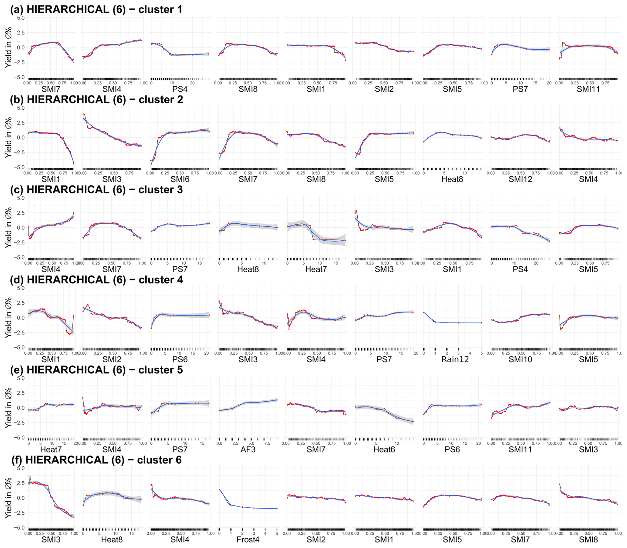
Figure A6 ALE plots for the second best combination of cluster algorithm and cluster size (HIERARCHICAL with six clusters) for a soil moisture index configuration that only considers the uppermost 25 cm. For the six clusters, the nine ALE plots with the highest feature importance are shown. The importance ranking is established with 50 repetitions. We have chosen a grid size of 50 to estimate the ALE plots, which allows us to reveal the true complexity of the model at the expense of shakiness. Therefore a non-linear smoothing function (LOESS – locally estimated scatterplot smoothing) is added in blue (with the confidence interval in grey). SMI represents the soil moisture index for the uppermost 25 cm of the soil column, PS stands for days without rain in a given month, Heat stands for days with a maximum temperature of more than 30 ^∘C, and Rain represents the days of precipitation higher than 30 mm/d. The number indicates the month; October (10) to December (12) refers to the year before.

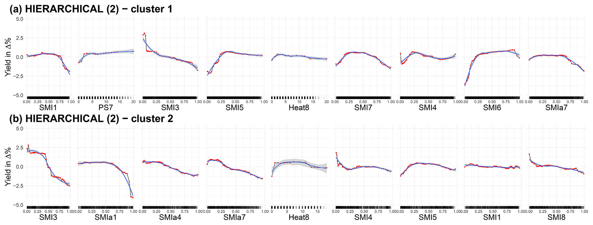
Figure A7 ALE plots for the best combination of cluster algorithm and cluster size (HIERARCHICAL with two clusters) for a soil moisture index configuration that considers both the uppermost 25 cm as well as the entire soil column. For both clusters, the nine ALE plots with the highest feature importance are shown. The importance ranking is established with 50 repetitions. We have chosen a grid size of 50 to estimate the ALE plots, which allows us to reveal the true complexity of the model at the expense of shakiness. Therefore a non-linear smoothing function (LOESS – locally estimated scatterplot smoothing) is added in blue (with the confidence interval in grey). SMI represents the soil moisture index for the uppermost 25 cm of the soil column, PS stands for days without rain in a given month, and Heat stands for days with a maximum temperature of more than 30 ^∘C. The number indicates the month; October (10) to December (12) refers to the year before.

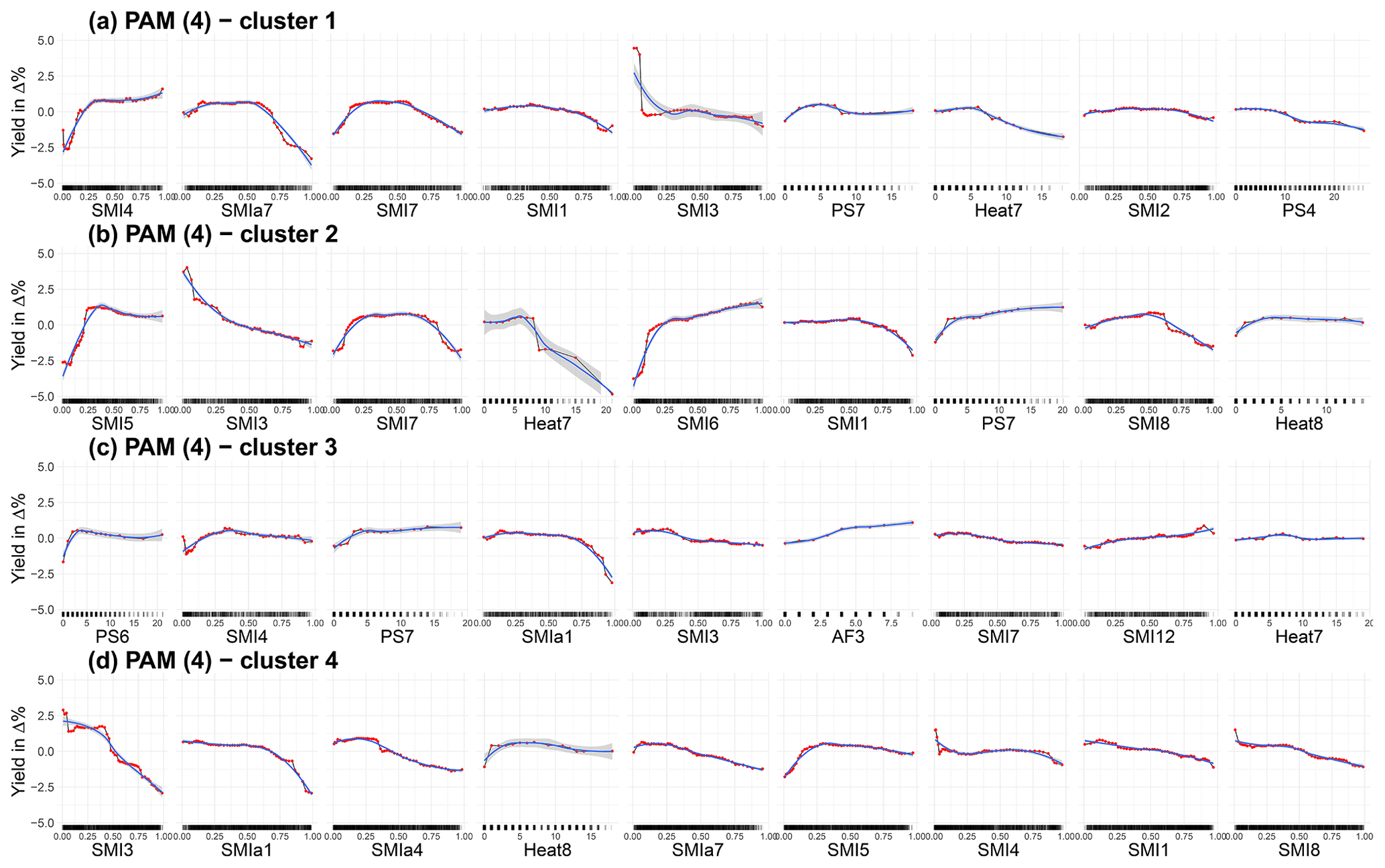
Figure A8 ALE plots for the second best combination of cluster algorithm and cluster size (PAM with four clusters) for a soil moisture index configuration that considers both the uppermost 25 cm as well as the entire soil column. For the four clusters, the nine ALE plots with the highest feature importance are shown. The importance ranking is established with 50 repetitions. We have chosen a grid size of 50 to estimate the ALE plots, which allows us to reveal the true complexity of the model at the expense of shakiness. Therefore a non-linear smoothing function (LOESS – locally estimated scatterplot smoothing) is added in blue (with the confidence interval in grey). SMI represents the soil moisture index for the uppermost 25 cm of the soil column, PS stands for days without rain in a given month, and Heat stands for days with a maximum temperature of more than 30 ^∘C. The number indicates the month; October (10) to December (12) refers to the year before.

Figure A9 ALE plots for the third best combination of cluster algorithm and cluster size (PAM with six clusters) for a soil moisture index configuration that considers both the uppermost 25 cm as well as the entire soil column. For the six clusters, the nine ALE plots with the highest feature importance are shown. The importance ranking is established with 50 repetitions. We have chosen a grid size of 50 to estimate the ALE plots, which allows us to reveal the true complexity of the model at the expense of shakiness. Therefore a non-linear smoothing function (LOESS – locally estimated scatterplot smoothing) is added in blue (with the confidence interval in grey). SMI represents the soil moisture index for the uppermost 25 cm of the soil column, PS stands for days without rain in a given month, and Heat stands for days with a maximum temperature of more than 30 ^∘C. The number indicates the month; October (10) to December (12) refers to the year before.