the Creative Commons Attribution 4.0 License.
the Creative Commons Attribution 4.0 License.
 | 13 Dec 2021
Optimizing a backscatter forward operator using Sentinel-1 data over irrigated land
Sara Modanesi
Christian Massari
Alexander Gruber
Hans Lievens
Angelica Tarpanelli
Renato Morbidelli
Gabrielle J. M. De Lannoy
Worldwide, the amount of water used for agricultural purposes is rising, and the quantification of irrigation is becoming a crucial topic. Because of the limited availability of in situ observations, an increasing number of studies is focusing on the synergistic use of models and satellite data to detect and quantify irrigation. The parameterization of irrigation in large-scale land surface models (LSMs) is improving, but it is still hampered by the lack of information about dynamic crop rotations, or the extent of irrigated areas, and the mostly unknown timing and amount of irrigation. On the other hand, remote sensing observations offer an opportunity to fill this gap as they are directly affected by, and hence potentially able to detect, irrigation. Therefore, combining LSMs and satellite information through data assimilation can offer the optimal way to quantify the water used for irrigation.
This work represents the first and necessary step towards building a reliable LSM data assimilation system which, in future analysis, will investigate the potential of high-resolution radar backscatter observations from Sentinel-1 to improve irrigation quantification. Specifically, the aim of this study is to couple the Noah-MP LSM running within the NASA Land Information System (LIS), with a backscatter observation operator for simulating unbiased backscatter predictions over irrigated lands. In this context, we first tested how well modelled surface soil moisture (SSM) and vegetation estimates, with or without irrigation simulation, are able to capture the signal of aggregated 1 km Sentinel-1 backscatter observations over the Po Valley, an important agricultural area in northern Italy. Next, Sentinel-1 backscatter observations, together with simulated SSM and leaf area index (LAI), were used to optimize a Water Cloud Model (WCM), which will represent the observation operator in future data assimilation experiments. The WCM was calibrated with and without an irrigation scheme in Noah-MP and considering two different cost functions. Results demonstrate that using an irrigation scheme provides a better calibration of the WCM, even if the simulated irrigation estimates are inaccurate. The Bayesian optimization is shown to result in the best unbiased calibrated system, with minimal chances of having error cross-correlations between the model and observations. Our time series analysis further confirms that Sentinel-1 is able to track the impact of human activities on the water cycle, highlighting its potential to improve irrigation, soil moisture, and vegetation estimates via future data assimilation.
- Article
(6088 KB) - Full-text XML
-
Supplement
(540 KB) - BibTeX
- EndNote


Over the last century, the global water withdrawal grew 1.7 times faster than the population (FAO, 2006). This aggravates the concern over the sustainability of water use as the demand for agricultural uses continues to increase (Foley et al., 2011; FAO AQUASTAT http://www.fao.org/nr/water/aquastat/water_use/index.stm, last access: 20 May 2021). The strong impact of irrigation on the global water budget is highlighted by many studies, and it has been estimated that about 87 % of the global fresh water withdrawals have been used for agriculture (Douglas et al., 2009). Accordingly, the quantification of irrigation on a regional to global scale has become a hot research topic.
Correctly quantifying irrigation in Earth system models can serve two purposes. On the one hand, it can help improve water management (Le Page et al., 2020, Bretreger et al., 2020); on the other hand, it allows us to quantitatively assess its effects on the terrestrial water, carbon, and energy cycles (Haddeland et al., 2007; Breña-Naranjo et al., 2014; Hu et al., 2016; Qian et al. 2020). Indeed, results of large-scale irrigation studies using land surface models (LSMs) have demonstrated that irrigation increases soil moisture and evapotranspiration (ET) and, consequently, latent heat flux with a decrease in sensible heat flux (i.e. Badger and Dirmeyer, 2015; Lawston et al., 2015; Ozdogan et al., 2010).
Despite the significant impact of irrigation on the water and energy cycles, its simulation within LSMs is not yet common practice (Girotto et al., 2017). In earlier studies, attempts to simulate irrigation in LSMs have relied on different parameterizations of well-known irrigation systems (like sprinkler, flood, and drip systems; Ozdogan et al., 2010; Evans and Zaitchik, 2008), making simplified assumptions. For instance, in Ozdogan et al. (2010), irrigation water is not withdrawn from a source (such as a river) but instead added as fictitious rainfall. In contrast, Nie et al. (2018) accounted for source water partitioning, albeit only partially, by considering groundwater irrigation. Irrigation is normally applied when soil moisture drops below a user-defined threshold (Ozdogan et al., 2010) and is typically dependent on the soil properties obtained via soil texture maps.
Moreover, LSMs equipped with irrigation schemes need to be provided with auxiliary information about crop types and whether or not the crops are irrigated. This is because different crop types are characterized by different rooting depths, which means they require more or less water to restore root zone field capacity. This information is normally gathered from static maps derived from statistical analysis and/or remote sensing (Ozdogan et al., 2010; Monfreda et al., 2008; Salmon et al., 2015) collected during specific historical periods, which are normally different to the desired period of analysis. It is thus clear that the modelling of irrigation is subject to many simplifying assumptions, which span from neglecting the year-to-year crop variability and the irrigation system used to the definition of irrigation application times based on water availability and crop conditions rather than actual farmer decisions.
Remote sensing (RS) technologies offer the opportunity to observe the Earth's surface and its changes directly and, hence, are potentially able to monitor irrigated lands worldwide (Ambika et al., 2016; Gao et al., 2018; Bousbih et al., 2018; Bazzi et al., 2019; Le Page et al., 2020; Dari et al., 2020). In the last decade, some authors used visible and near-infrared RS observations jointly with in situ data collected from inventories to map areas equipped for irrigation (Ambika et al., 2016; Ozdogan and Gutman, 2008). S. V. Kumar et al. (2015) were the first to propose the use of coarse resolution satellite microwave (MW) sensors to detect irrigation. The authors compared different coarse-scale active and passive MW surface soil moisture (SSM) retrievals with SSM simulations from the Noah LSM (version 3.3; Ek et al., 2003) without activating an irrigation scheme over a continental USA domain. Areas where the distributions of model and RS data sets deviated (based on a Kolmogorov–Smirnov test) were assumed to be irrigated. Even though some of the products showed a potential ability to detect irrigation, the authors concluded that the spatial mismatch between the satellite footprint and the irrigated fields, radio frequency interference (RFI), vegetation, and topography could all deteriorate the accuracy of the results. Similar conclusions were found over the same area by Zaussinger et al. (2019), who compared coarse-scale satellite SSM products with soil moisture predictions from the Modern-Era Retrospective analysis for Research and Applications, version 2 (MERRA-2) in the absence of precipitation, and Escorihuela and Quintana-Seguí (2016), who additionally compared a downscaled version of the Soil Moisture and Ocean Salinity (SMOS) mission SSM to SURFEX LSM simulations. Brocca et al. (2018), Jalilvand et al. (2019), and Dari et al. (2020) used a conceptually different approach, with the same coarse scale MW SSM products, and estimated irrigation by directly inverting a simple water balance equation (Brocca et al., 2014).
The Copernicus Sentinel-1 satellites (Sentinel-1A and Sentinel-1B) offer a new perspective for agricultural applications thanks to the finer spatial resolution (up to 10–20 m) of the synthetic aperture radar (SAR) backscatter (σ0) data. For instance, Gao et al. (2018) proposed an approach to map irrigated lands over the Urgell region in Catalonia (Spain), and Le Page et al. (2020) proposed a methodology to detect irrigation timing in southwestern France by comparing the SSM signal at the plot scale, derived using Sentinel-1 σ0 and NDVI from Sentinel-2 (El Hajj et al., 2017), with a water budget model forced by Sentinel-2 optical data for the detection of irrigation timing.
Despite the high potential demonstrated by RS in detecting, mapping, and quantifying irrigation, the uncertainties of the satellite retrievals, the relatively low revisit time of high-resolution active MW products, and the too coarse spatial resolution of passive MW products with respect to the mean size of irrigated fields represent main limitations for irrigation information retrieval (Romaguera et al., 2010; La Page et al., 2020). Data assimilation (DA) could reduce some uncertainties by optimally integrating LSM estimates and RS observations. Indeed, the LSM estimates resolve processes at desired spatiotemporal scales, while the RS observations can track, in a more realistic way, human processes like irrigation and their interactions with the water and energy cycles. Contrasting LSM simulations with RS observations offers an opportunity to correct for unmodelled processes or missed events, such as irrigation (S. V. Kumar et al., 2015; Girotto et al., 2017). More generally, DA of satellite-based observations has shown the potential to update soil moisture (De Lannoy and Reichle, 2016; Kolassa et al., 2017) and vegetation (Albergel et al., 2018; Kumar et al., 2020), and important impacts have been reported over agricultural areas (Kumar et al., 2020).
The assimilation of MW RS observations in LSMs often involves retrieval assimilation. However, assimilating retrievals (i.e. SSM or vegetation optical depth rather than MW brightness temperature or σ0 measurements) can be problematic as the retrievals may have been produced with ancillary data that are inconsistent with those used in the LSM (De Lannoy et al., 2016). This is particularly true for passive MW retrievals, while active MW retrievals generally rely on change detection methods that lack land-specific ancillary information altogether. An alternative approach, which we follow in this study, is to directly assimilate MW observations and equip the LSM with an observation operator that links the land surface variables of interest (e.g. soil moisture and vegetation) with RS data. This allows us to obtain consistent parameters and to reduce the chance of cross-correlated errors between model states and corresponding geophysical satellite retrievals. The direct assimilation of MW observations has already been demonstrated successfully for the update of soil moisture by using brightness temperature (Tb) derived from the SMOS and SMAP (Soil Moisture Active Passive) missions (De Lannoy et al., 2016; Carrera et al., 2019; Reichle et al. 2019), as well as using radar σ0 from ASCAT (Advanced Scatterometer; Lievens et al., 2017b), and σ0 from Sentinel-1 in synergy with SMAP Tb (Lievens et al., 2017a). However, to our knowledge, none of these studies considered the joint updating of soil moisture and vegetation, and none specifically focused on the performance over irrigated areas. The σ0 from Sentinel-1 contains information on both soil moisture (Zribi et al., 2011; Liu and Shi, 2016; Li and Wang, 2018; Bauer-Marschallinger et al., 2018) and vegetation (Vreugdenhil et al., 2018, 2020), and assimilating this data could allow us to update both soil moisture and vegetation in a land data assimilation system and, in doing so, correct for missed irrigation events.
To that end, the LSM needs to be coupled to a backscatter forward model as an observation operator. Different SAR σ0 models have been proposed to simulate the backscattering contributions of soil and vegetation (Attema and Ulaby, 1978; Oh, 2004; Zribi et al., 2005; Bai et al., 2015; Baghdadi et al., 2017). Most commonly used, the Water Cloud Model (WCM hereafter) developed by Attema and Ulaby (1978) is a σ0 model that represents the vegetation canopy as a homogeneous cloud containing randomly distributed water droplets. In order to use the WCM as the forward operator in a σ0 data assimilation system, it first needs to be calibrated to account for biases between the LSM simulations and the satellite observations. However, calibrating a WCM to simulate σ0 over irrigated areas is not a straightforward process, and it represents a key research problem if the same σ0 signal is used for the calibration of WCM parameters and later for assimilation and updating of the state. In fact, if the objective is to assimilate radar σ0 to realistically inform the model about irrigation applications, the WCM parameters have to maintain a certain degree of independence from the irrigation signal contained in the observed σ0 as, otherwise, the assumption of uncorrelated errors between model and observations typical of classical Bayesian-based filters is violated. More specifically, if the LSM provides unrealistic simulations as input (i.e. the absence of irrigation), then the WCM calibration with observed σ0 would compensate for this bias. This would, in turn, lead to a biased backscatter model with undesirable calibrated parameters for the subsequent data assimilation experiments. Therefore, different strategies can be adopted, for instance by calibrating the model during non-irrigated periods or over non-irrigated areas or equipping the LSM with an irrigation module that makes the WCM less constrained by inconsistencies between simulated and observed σ0 during irrigation periods. The efficacy of these strategies has, so far, never been explored.
The main objective of this study is to simulate radar σ0 using a LSM coupled with a WCM and to provide solutions and recommendations for the optimization of the WCM as an observation operator. This is a major stepping stone towards the development of a reliable system for the assimilation of high-resolution Sentinel-1 σ0 observations over irrigated areas. Additionally, we aim at the following:
-
testing the ability of a sprinkler irrigation system coupled with a LSM to simulate irrigation so as to highlight the potential and limitations of such a tool to optimize a backscatter forward operator over heavily irrigated areas
-
demonstrating that Sentinel-1 σ0 observations contain valuable information to improve both SM and vegetation predictions over irrigated land (i.e. soil moisture and vegetation consistent with human alterations in the water cycle due to intensive irrigation).
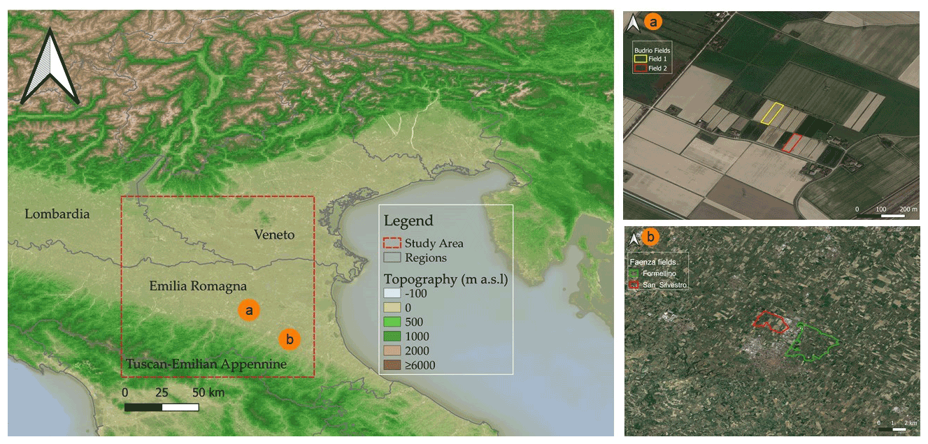
Figure 1The study area and the two test sites of (a) Budrio and (b) Formellino. Data on the topography are obtained from ETOPO1 Arc-Minute Global Relief Model (Amante and Eakins, 2009). Map data © 2015 Google.
The analysis is carried out over the Po Valley, one of the most important agricultural areas in Italy and also one of the more intensively irrigated areas in Europe (water withdrawal in the Po basin is estimated to be 20.5 billion m3 yr−1, of which 16.5 billion m3 yr−1 is withdrawn for irrigation; Po River Watershed Authority, 2016). We use the Noah-MP v.3.6 LSM (Noah-MP hereafter) as part of the NASA Land Information System (LIS) framework, together with the WCM from Attema and Ulaby (1978), for the simulation of both σ0 vertical send and receive (VV) and vertical send and horizontal receive (VH) polarization. Level 1 Sentinel-1 σ0 observations are used to calibrate the WCM at 1 km resolution, using simulated SSM and leaf area index (LAI) estimates from Noah-MP. The WCM is calibrated for a total of four calibration experiments for each polarization, namely (1) with or without activating an irrigation scheme within Noah-MP and (2) considering two different cost functions. Specifically, we want to demonstrate that activating an – even poor – irrigation scheme is needed to obtain long-term unbiased σ0 simulations and uncorrelated errors between the WCM and Sentinel-1, and that the calibration process can be sensitive to different cost functions.
The paper is organized as follows. Section 2 provides information on the study area, the selected data sets, and methods used for our analysis. Specifically, Sect. 2.3 and 2.4 provide a detailed description of the Noah-MP LSM and the WCM. Section 2.5 describes the cost functions used for the WCM calibration, while Sect. 2.6 is a description of the experimental set-up designed for the calibration. Finally, Sect. 2.7 provides insights on the Noah-MP and WCM evaluations. Section 3 presents the results, with an assessment of the Noah-MP evaluation, both regional (Sect. 3.1) and over the test sites (Sect. 3.2). The WCM calibration and evaluation results are described in Sect. 3.3 and 3.4, respectively. We provide a discussion in Sect. 4, while conclusions are reported in Sect. 5.
2.1 Study area and in situ data
The analysis was carried out over an area of 24 000 km2 located within the Po Valley, one of the most important agricultural areas in Europe (Fig. 1; 44∘ N, 10.5∘ W – bottom left; 45.5∘ N, 12.2∘ W – top right). The Po Valley is part of the Po basin district (∼ 74 000 km2), a mountain-fed catchment which extends from the Alps in the west to the Adriatic Sea in the east. The Po district is one of the eight districts mentioned in the Water Framework Directive (WFD; EC, 2000) initiated by the European Commission and has been hit by seasonal drought events which impacted all water use sectors, in particular agriculture (Strosser et al., 2012). The water assessment and impact evaluation of human activities over the Po Valley is thus a topic of major interest, considering the significant requirements from the agricultural management sector.
According to the Köppen–Geiger climate classes (Peel et al., 2007) the study area is classified as Cfa (temperate climate, without a dry season, and with hot summers). From a geographical point of view, the Po river flows from the west to the east, splitting the area of interest in northern and southern areas, respectively. North of the Po river, the agricultural plain area can additionally be subdivided into the Veneto region to the east and the Lombardy region to the west (Fig. 1). Lombardy lands have a high water availability, thanks to the presence of several Alpine lakes and reservoirs (Musolino et al., 2017), as does the Veneto region. Wine cultivation plays an important role, especially in the Lake Garda surroundings (located to the northwest of the study area). In the south, the Emilia Romagna region is an agricultural and urbanized industrialized area. Compared to Lombardy and Veneto, Emilia Romagna is much poorer both in water availability and storage capacity, but its irrigation system is considered the most technologically advanced and efficient in the Po river basin (Musolino et al., 2017). Specifically, it hosts the Canale Emiliano Romagnolo (CER; https://consorziocer.it/it/, last access: 20 May 2021), which is one of the most important Italian hydraulic systems for agricultural water supply. The main crops in the study region include general summer and winter crops, orchards (i.e. peach, pear, and kiwi), olive groves, and vineyards (https://sites.google.com/drive.arpae.it/servizio-climatico-icolt/home; last access: 20 May 2021). The plain area is surrounded by a forested hilly and mountainous area of the Tuscan–Emilian Apennines to the south/southwest.
In situ data were collected over two test sites located in the Emilia Romagna region.
-
For an analysis at plot scale, we selected the Budrio test site (Fig. 1a), an experimental farm managed by the CER authority, which includes two plots of 0.39–0.49 ha. The main crops are maize for field 1 (in yellow) and tomatoes in field 2 (red). Daily irrigation data, in millimetres, were collected for the summer of 2015–2016 over field 1, whereas daily irrigation water amounts were collected for the summer of 2017 over field 2. Additionally, for field 2, hourly in situ soil moisture data, aggregated here at a daily scale, were made available from the Department of Physics and Earth Science of the University of Ferrara. The soil moisture data were derived from an innovative proximal gamma-ray (PGR SM hereafter; Filippucci et al., 2020, Strati et al., 2018) station, equipped with a 1 L NaI(Tl) detector placed at 2.25 m above ground and a commercial agro-meteorological station (MeteoSense 2.0, Netsens; Strati et al., 2018). The PGR is a nuclear non-invasive and non-contact technique, which allows us to overcome the issue connected to in situ point measurements, probing soil moisture with a field-scale footprint (∼ 104 m2) up to a depth of ∼ 30 cm. The quantification of PGR soil moisture is derived from measurements of gamma signals emitted by the decay of 40K, which is extremely sensitive to different soil water contents in agricultural soils (for more information on the PGR soil moisture deriving procedure, the reader can refer to Baldoncini et al., 2019). Finally, daily rainfall data were collected from the national rainfall network, managed by the Department of Civil and Environmental Protection (DPC) of Italy, for the irrigated periods.
-
The second test site (Fig. 1b) is located around the city of Faenza (hereafter the Faenza test site) and has a total extent of 1051 ha, consisting of two fields which allow analysis at the small-district spatial scale. The first one is called San Silvestro (290 ha), and it is located north of the city. The second one is called Formellino (760 ha), located east of the San Silvestro field and northeast of the city of Faenza. Fruit trees are prevalent on the fields; in particular, pear trees and kiwi dominate the area. The water used for irrigation was provided by CER, at an hourly timescale and in millimetres, for the 2-year time period of 2016–2017. Daily rainfall data were collected from the national rainfall network managed from the DPC.
2.2 Sentinel-1 σ0 and reference remote sensing products
The Copernicus-ESA Sentinel-1 σ0 observations were used in this study for the calibration of the WCM. The Sentinel-1 constellation consists of two satellites, Sentinel-1A and Sentinel-1B, launched in 2014 and 2016, respectively. Each satellite carries a synthetic aperture radar (SAR) operating at the C band (5.4 GHz) in the microwave portion of the electromagnetic spectrum. The processing of the ground-range detected (GRD) interferometric wide swath (IW) observations in VV and VH polarization was done using Google Earth Engine's Python interface and included standard techniques, namely precise orbit file application, border noise removal, thermal noise removal, radiometric calibration, and range Doppler terrain correction. Furthermore, the σ0 observations acquired at 5 m × 20 m resolution were aggregated and projected on the 1 km Equal-Area Scalable Earth version 2 (EASE-2) grid (Brodzik et al., 2012). After applying an orbit bias correction (Lievens et al., 2019), the observations from different orbits, either from Sentinel-1A or Sentinel-1B and ascending or descending tracks, were combined at the daily timescale.
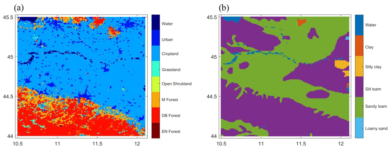
Figure 2Regridded and reclassified input data used in the LIS framework. (a) The PROBA-V land cover (LC) map. (b) The Harmonized World Soil Database (HWSD) soil texture map.
Additionally, RS observations were used for the evaluation of the SSM and LAI simulated in Noah-MP LSM for the period 31 March 2015–December 2019.
-
The NASA Soil Moisture Active Passive (SMAP; Entekhabi et al., 2010) is an orbiting observatory launched in January 2015 carrying two instruments, namely a SAR, which suffered a failure in early July 2015, and a radiometer measuring Tb at the L band, with a native spatial resolution of 40 km, a revisit time of 2–3 d, and ascending and descending overpasses at 18:00 and 06:00 LT (local time), respectively. For this study, the 9 km SMAP Enhanced Level-2 SSM version 4 (0–5 cm; SMAP L2 hereafter) product was used (O'Neill et al., 2020; Chan et al., 2018). The product is derived from SMAP Level-1B (L1B) interpolated antenna temperatures using the Backus–Gilbert optimal interpolation technique. Both ascending and descending tracks were collected.
-
The Metop ASCAT SSM Climate Data Record (CDR) H115 and its extension H116 are provided by the European Organization for the Exploitation of Meteorological Satellites (EUMETSAT) Support to Operational Hydrology and Water Management (H SAF, 2021). The SSM is retrieved from σ0, using a change detection algorithm (Wagner et al., 2013), and is characterized by a spatial sampling of 12.5 km and a temporal resolution of one to two observations per day, depending on the latitude.
-
The PROBA-V LAI is derived from the PROBA-V satellite mission (Francois et al., 2014; Dierckx et al., 2014) and provided by the Copernicus Global Land Service (CGLS) programme (Copernicus Global Land Service Site, 2021). The CGLS product at 1 km spatial resolution and 10 d temporal resolution is developed based on the work by Verger et al. (2014).
In order to compare Noah-MP simulations and reference data at the same spatial resolution, Sentinel-1 observations (σ0 VV and σ0 VH) and ASCAT SSM, SMAP L2 SSM, and PROBA-V LAI were extracted over the study domain (44∘ N, 10.5∘ W – bottom left; 45.5∘ N, 12.2∘ W – top right) and regridded over the LIS grid domain (0.01∘) using the nearest neighbour approach.
2.3 Land surface and irrigation modelling
2.3.1 Noah-MP v.3.6
The analysis was carried out using the Noah-MP (Niu et al., 2011) LSM, running within NASA's LIS version 7.2 (Kumar et al., 2008). LIS is a software framework for terrestrial hydrology modelling and DA, which supports different LSMs that can be conditioned on multiple remote sensing products from active and/or passive microwave sensors. The Noah-MP LSM, which was chosen for this study, is an evolution of the baseline Noah LSM (Mahrt and Ek, 1984; Chen et al., 1996; Chen and Dudhia, 2001), where the main improvements and augmentations are (1) the presence of four soil layers, (2) up to three snow layers, (3) one canopy layer, which allows us to dynamically simulate the vegetation and to compute separately the ground surface temperature, (4) a two-stream radiation transfer scheme based on the canopy layer sub-grid scheme, (5) a Ball–Berry-type stomatal resistance scheme, and, (6) finally, a simple groundwater model with a TOPMODEL-based runoff scheme (Niu et al., 2005, 2007). The model was set up by selecting four soil layers at depths of 0–10, 10–40, 40–100, and 100–200 cm, a dynamic vegetation model with a Ball–Berry-type canopy stomatal resistance model (Ball et al., 1987), and TOPMODEL-based runoff.
The parameterization followed the recommended options provided in the LIS documentation (https://lis.gsfc.nasa.gov/documentation/lis, last access: 30 November 2021). A model time step of 15 min and a 6 h output interval were selected, together with a spatial resolution of 0.01∘. The meteorological forcings used for running Noah-MP LSM were obtained from MERRA-2 (Gelaro et al. 2017). The MERRA-2 original spatial resolution of 0.5∘ × 0.625∘ was remapped to 0.01∘ through bilinear interpolation. Land model data and parameters were preprocessed and adapted to the LIS longitude/latitude projection using the Land Surface Data Toolkit (LDT; Arsenault et al., 2018) in order to run Noah-MP at the chosen spatial resolution.
For this study, the default LIS land cover (LC) map from the University of Maryland (UMD) global land cover product (Hansen et al., 2000), based on the Advanced Very High Resolution Radiometer (AVHRR) data, was replaced with the 2015 global LC map, available from the CGLS at 100 m spatial resolution (Buchhorn et al., 2020; available at https://land.copernicus.eu/global/products/lc, last access: 20 May 2021). The CGLS provides dynamic land cover layers at 100 m spatial resolution (CGLS-LC100), obtained by combining information derived from the vegetation instrument on board the PROBA-V satellite, a database of high-quality LC reference sites, and several ancillary data sets. For a more detailed explanation of the LC maps generation process we refer to the Algorithm Theoretical Basis Document (ATBD; Buchorn et al., 2020). The 23 classes of the PROBA-V LC map were reclassified to the 14 classes used in the UMD-AVHRR classification supported by LIS. Additionally, the LC map was regridded at 0.01∘ (Fig. 2a) by identifying the most representative class over each LIS grid cell. For additional information on the reclassification process, we refer the reader to Table S1 in the Supplement. Similarly, the default Food and Agriculture Organization (FAO) Soil Map (FAO, 1971) was replaced by the Harmonized Soil World Database (HWSD v1.21; 1 km; Fig. 2b) and mapped to five soil classes over the study region. Other model preprocessed parameters inputs were (1) the Shuttle Radar Topography Mission elevation data (SRTM30; 30 m spatial resolution); (2) the climatological global Greenness Vegetation Fraction (GVF) data (0.144∘; Gutman and Ignatov, 1998), derived from 5 years (1985–1989) of normalized difference vegetation index (NDVI) data from the AVHRR (Miller et al., 2006), (3) a snow-free albedo and a Noah-specific maximum snow albedo product from NCEP (National Centers for Environmental Prediction; original resolution 1∘ and regridded), and, finally, (4) soil, vegetation, and other general parameter tables for Noah-MP from the official LIS Data Portal (https://portal.nccs.nasa.gov/lisdata_pub/data/, last access: 20 May 2021).
2.3.2 Irrigation modelling
The ability of Noah-MP to dynamically simulate the vegetation and the option to activate irrigation are particularly important when considering an extensively irrigated area such as the Po Valley. Indeed, in a recent study by Nie et al. (2018), Noah-MP was coupled with a sprinkler irrigation scheme (Ozdogan et al., 2010; where irrigation is applied as supplementary rainfall), which requires the following three pieces of information:
-
The irrigation location, which only occurs over potentially irrigated croplands (expanding over grassland if the intensity exceeds the grid cell's total crop fraction). This information is extracted from a LC map associated with an additional data set providing information on the percent of irrigated area per grid cell. In this study, the reclassified PROBA-V LC map was coupled with the information contained in the 500 m global rain-fed, irrigated, and paddy croplands data set (GRIPC; Salmon et al., 2015).
-
The timing of irrigation, which is determined by checking the start and end of the growing season, based on a GVF threshold, separately at each grid cell. Following Ozdogan et al. (2010), we set this threshold to 40 % of the GVF.
-
The amount of water which is used for irrigation. This quantity is derived from the root zone soil moisture (RZSM) availability (MA) as , where RZSM is the current RZSM, SMWP is the wilting point, and SMFC is the field capacity. When the MA falls below a user-defined threshold, irrigation is triggered, and the quantity is defined by calculating the amount of irrigation needed to raise the RZSM to the SMFC. For this study, the MA threshold was defined as the 50 % of SMFC as in Ozdogan et al. (2010). MA is calculated at each time step, but the irrigation is only applied between 06:00 and 10:00 LT. Following Ozdogan et al. (2010), this time frame is typically chosen by farmers to reduce evaporative losses. In this context, the maximum rooting depth becomes a crucial information to compute the amount of irrigation water. This information is related to an assigned crop type, cultivated over the study area, through a maximum rooting depth table. Considering the high crop variability over the Po Valley and the lack of high-resolution dynamic crop maps for the entire study area, a generic crop type with 1 m root depth was selected for the irrigation simulations. The reference rooting depth was verified to be feasible over the study area, based on the European Soil Data Centre (ESDAC; available at https://esdac.jrc.ec.europa.eu/content/european-soil-database-derived-data, last access: 20 May 2021) rooting depths map (Fig. S1 in the Supplement).
2.4 Water Cloud Model
The WCM allows us to simulate the top-of-vegetation σ0 as a function of SSM and vegetation, using empirical fitting parameters. σ0 is modelled as the sum of the backscatter from the vegetation (; in decibels, hereafter dB) and from the bare soil (; in dB), attenuated by the t2 coefficient that describes the two-way attenuation from the vegetation layer. Scattering interactions between the ground and the vegetation are not accounted for. As reported in Baghdadi et al. (2017), for a given polarization pq (i.e. VV and VH), the WCM can be written as follows:
where, in the following,
Equations (2) and (3) describe the vegetation-related terms. V1 and V2 represent two bulk vegetation descriptors, with the first one accounting for the direct vegetation σ0 and the second one representing the attenuation. Apq (−) and Bpq (−) are the two related fitting parameters. Common vegetation descriptors used in previous studies are the vegetation water content (VWC; Paloscia et al., 2013), the NDVI (El Hajj et al., 2016; Li and Wang, 2018), and LAI (K. Kumar et al., 2015; Bai and He, 2015), while θ represents the incidence angle, which is assumed to be 37∘ for Sentinel-1. Following previous studies (see Lievens et al., 2017b; Baghdadi et al. 2017; Li and Wang, 2018), we assumed V1=V2 represented by the dynamically simulated LAI vegetation descriptor.
Equation (4) describes the soil-related term. Following the work by Lievens et al. (2017b), the can be described, in a simple linear approach, as a function of the SSM. There are several semi-empirical models (e.g. the Oh model; Oh et al., 1992) or theoretical models (e.g. the Integral Equation Model – IEM; Fung, 1994), which describe the scattering processes related to the bare soil, but their application as a forward operator coupled to a LSM has two main limitations. The first one lies in the difficulty in retrieving soil roughness values over extended reference areas required to parameterize these models. The second one is their saturation of σ0 in moist conditions, which causes low variability in simulated σ0 if the LSM soil moisture simulations are biased wet (for more information, see Lievens et al., 2017b). Those limitations justify the use of a linear fitted approach. In Eq. (4), the C and D parameters (here fitted in dB and decibels per cubic metre per cubic metre, , respectively, but is transformed back to the linear scale in Eq. 1) describe the linear relation between and SSM. Those parameters, together with A and B (–), need to be calibrated separately for each polarization.
2.5 Calibration algorithms
We considered the following two different objective functions to optimize the A, B, C, and D parameters:
-
A Bayesian solution, which minimizes the sum of squared errors (SSEs) between σ0 observations from Sentinel-1 and WCM simulations. The SSE Bayesian calibration solution aims at identifying the optimal parameter vector α, which maximizes the probability of the resulting σ0 simulations , where p(α) is the prior parameter distribution and is the likelihood. Starting from the assumption of an independent and identically distributed normal error model, the posterior probability can be maximized by maximizing the following:
i.e. the combination of the likelihood and a prior parameter constraint. The latter helps in reducing problems of equifinality. In Eq. (5), represents the observed σ0, is the simulated σ0, i is the time step, and si is the standard deviation of the residual differences between the observed and simulated σ0 values for Ni time steps. Nα is the number of parameters to be calibrated, α0 is the prior parameter constraint, and the parameter deviation is limited by , which is the variance of a uniform distribution , with determined boundaries of the parameters []. The maximum likelihood solution is found by minimizing the following cost function J:
where si is assumed to be constant in time and represented by a target accuracy of 1 dB, leaving the SSEs in the first term of J0 to minimize. The second term (Jα) constrains the optimal solution by avoiding strong deviations from initial parameter guesses.
-
A solution that maximizes the Kling–Gupta efficiency (KGE; Gupta et al., 2009). Even though this objective function does not ensure Bayesian optimality, it is a widely used metric which could help to better tune the dynamic σ0 behaviour, as follows:
The KGE formulation embeds three terms. (1) The first term accounts for the Pearson correlation (Pearson R) between the observed () and simulated () σ0 time series. (2) A second term accounts for the bias, where the long-term mean is represented as 〈.〉. Finally, (3) there is a term accounting for the variability in the simulated and observed signal through the use of the standard deviation s[.]. KGE = 1 indicates a perfect agreement between simulations and observations. Note that KGE redistributes the weight of the bias, variance, and correlation components compared to J in Eq. (6), which can help in reducing differences between simulated and observed σ0, and also in terms of temporal dynamics, during the calibration. On the other hand, in the KGE, cost function parameters are not constrained by prior values α0. This could possibly result in overfitting and a larger prediction uncertainty.
The particle swarm optimization (PSO; Kennedy and Eberhart, 1995) was used to minimize J and maximize KGE. For our case study, the PSO parameters were set as in De Lannoy et al. (2013).
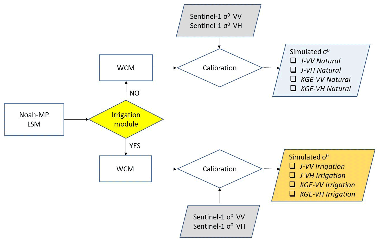
Figure 3Flow chart of the experimental set-up used in this study to calibrate the WCM σ0 signal. A natural and an irrigation experimental line was performed coupling either Noah-MP natural or irrigation simulations with the WCM. For each experimental line, σ0 simulations are driven by the Sentinel-1 signal using two different cost functions (J and KGE) in order to provide eight different calibration experiments.
2.6 Experimental set-up
An optimal DA system requires long-term unbiased σ0 simulations (with respect to the assimilated observations). The risk, over an intensively irrigated area, is that an unmodelled irrigation signal would manifest itself as a predominant bias in the σ0 simulations. The calibration would then inadvertently correct for this supposed bias (i.e. the irrigation signal), thus preventing the DA system from propagating the missing irrigation signal from the observations into the model. Even though existing irrigation schemes are evidently unrealistic and inaccurate, we conjecture that using such a scheme when calibrating the WCM will more likely yield optimal WCM parameters than when neglecting irrigation.
To that end, we considered two different experiment lines (referred to as natural and irrigation, respectively) that produced a total of eight different σ0 simulation runs (see Fig. 3). The natural experiment line differs from the irrigation line by the activation of an irrigation module in Noah-MP, and both are subjected to the calibration algorithms described in Sect. 2.5. The natural line was used as a diagnostic experiment against which to compare irrigation, which, according to our initial hypothesis, should minimize the impact of the irrigation signal contained in the σ0 observations on WCM parameters.
As a first step, a model spin up was performed, starting in January 1982 and ending in December 2014. Then, a study period from January 2015 to December 2019 was selected for the different model runs, based on the availability of the processed Sentinel-1 σ0 and reference irrigation data (see Sect. 2.1 and 2.2). Daily surface model and irrigation outputs were produced. Considering that the main source of irrigation in the Po Valley is related to surface water abstraction, the sprinkler irrigation scheme did not account for groundwater withdrawals (see Nie et al., 2018).
The A, B, C, and D parameters of the WCM (see Sect. 2.4) were fitted separately to Sentinel-1 σ0 VV and σ0 VH observations during the period of January 2017– December 2019. Following previous literature (Lievens et al., 2017b; De Lannoy et al., 2014, 2013), we performed a grid-cell-based calibration to account for the spatial variability in the simulated and observed σ0 signals that stems from specific features within the observed footprints and from the soil and vegetation parameterization of Noah-MP. Both the calibration using the SSEs with prior constraint (Bayesian J) and the KGE were applied to the natural and irrigation runs, providing eight different experiments named J-VV natural, J-VH natural, J-VV irrigation, J-VH irrigation, KGE-VV natural, KGE-VH natural, KGE-VV irrigation, and KGE-VH irrigation.
Table 1Lower boundaries (LB), upper boundaries (UB), and prior guess values of the WCM parameters for both VV and VH polarization.
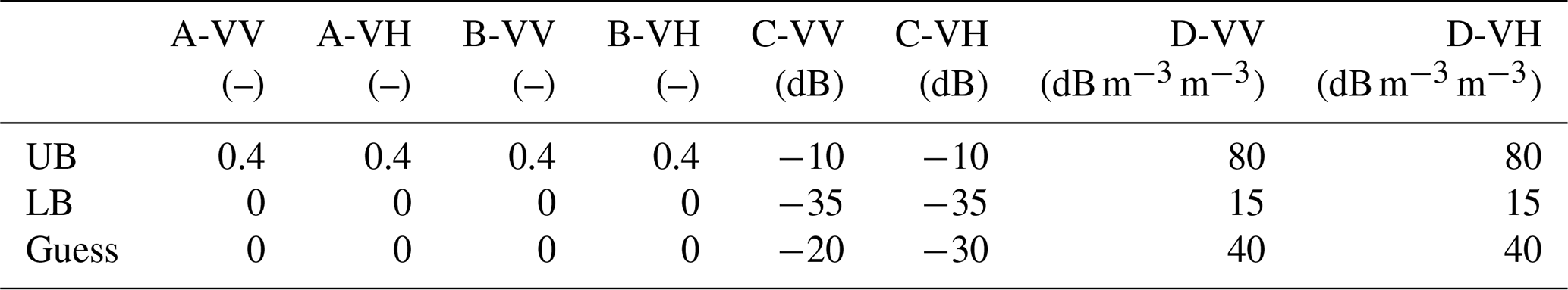
Lower and upper boundaries and prior guess values of the WCM parameters were defined based on the work of Lievens et al. (2017b) and on a sensitivity analysis (not shown here). The selected values are displayed in Table 1. Finally, it should be noted that all the calibration experiments were realized by considering daily values of σ0 simulations and observations.
2.7 Noah-MP LSM and WCM evaluations
The validation aims at (i) evaluating the performance of Noah-MP in simulating irrigation, soil moisture, and vegetation, and the ability of the WCM to simulate radar σ0, and (ii) unveiling the information about irrigation contained in Sentinel-1 radar σ0 in order to assess its potential to improve both soil moisture and vegetation representation within Noah-MP.
The evaluation was carried out on both the regional scale (i.e. over the entire study area) and on the two selected sites, Faenza (small district scale) and Budrio (plot scale), where irrigation data were available. Considering the lack of benchmark data for irrigation evaluation (Foster et al., 2020), we decided to use in situ data for the small Budrio fields spatial scale (i.e. 0.45–049 ha), even though model simulations are made at a much coarser resolution (i.e. ∼ 1 km). We are aware that differences in the spatial scale can increase the uncertainty of our evaluation, but the 0.01∘ LSM spatial resolution is still a good compromise for an analysis at the regional, small district, and plot scale. Additionally, limitations are partly reduced by the low chance of including non-irrigated fields within the 1 km LIS grid cells within the Po Valley, as the latter is almost entirely irrigated (Salmon et al., 2015). We compared Noah-MP (with and without using the irrigation module) SSM and LAI simulations with satellite SSM from ASCAT and SMAP and LAI from PROBA-V, respectively, during the period 2015–2019. Furthermore, these land surface simulations were compared to Sentinel-1 σ0 to understand how much of the SSM and LAI signal was captured by Sentinel-1.
As the irrigation timing is often driven by the stakeholders' turns to withdraw water and by water availability rather than by the conditions of the soil and crops themselves, the comparisons between simulated SSM and satellite SSM were carried out by aggregating the two variables over a biweekly time window. On the other hand, the LAI from Noah-MP was aggregated to 10 daily values in order to match the PROBA-V LAI values. We used the Pearson R for SSM and LAI evaluation. For SSM, we also computed the root mean square error (RMSE), calculated considering the original temporal resolution of the satellite products, while for LAI, we also tested the ratio bias, i.e. the ratio between the long-term mean of the simulations and the long-term mean of observations. In particular, this additional score for LAI was used to provide a further evaluation of the ability of the Noah-MP to simulate crop phenology during the irrigated vs. non-irrigated periods so as to not rely solely on the evaluation of temporal dynamics, which, due to the uncertainty in the Noah-MP crop type parameterization, could be affected by time shifts in the LAI climatology. This parameterization uncertainty comes from the lack of knowledge of the spatial crop type information and is difficult to reduce without additional information. Our assumption is that the radar σ0 assimilation can also correct for this with future data assimilation.
Following Vreugdenhil et al. (2018) and Vreugdenhil et al. (2020), Noah-MP LAI and PROBA-V LAI were also compared with the Sentinel-1 cross ratio (CR), which was demonstrated to have a high agreement with the vegetation signal. Though the σ0 VH was demonstrated to increase with the vegetation signal (Macelloni et al., 2001), the CR will be more sensitive to vegetation changes as the ratio is less sensitive to changes in soil moisture and soil–vegetation interaction (Veloso et al., 2017; Vreugdenhil et al., 2020).
To evaluate WCM simulations, we used biweekly values of σ0 simulations and observations considering a 2-year period independent from the calibration period (i.e. 2015–2016). Statistical metrics, such as grid-based temporal Pearson R, KGE, and bias, were calculated between Sentinel-1 σ0 and calibrated WCM simulations. The analysis of the parameters was restricted to the cropland area as no difference between our experiment lines exists over other land cover types (i.e. the irrigation module is active only over grid points classified as crop).
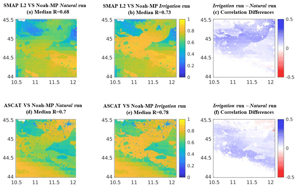
Figure 4Maps of temporal Pearson R between biweekly values of SSM from Noah-MP and satellite retrievals. (a) Natural run and SMAP L2. (b) Irrigation run and SMAP L2. (d) Natural run and ASCAT. (e) Irrigation run and ASCAT. Maps of the Pearson R differences display the grid-based difference between (c) map b and map a and (f) map e and map d. The reference period is April 2015–December 2019.
3.1 Noah MP regional evaluation
Figure 4 shows maps of the Pearson R between biweekly Noah-MP SSM natural and irrigation simulations and biweekly ASCAT and SMAP L2 SSM retrievals, respectively, for April 2015 to December 2019. The Noah-MP SSM irrigation run provides a higher agreement with both satellite SSM data sets compared to the natural run. Indeed, the median Pearson R between SMAP L2 SSM and Noah-MP SSM increases from 0.68 to 0.73, for the natural run (Fig. 4a) and the irrigation run (Fig. 4b), respectively. A similar improvement can be observed considering the ASCAT reference SSM, with an improvement in the median Pearson R of 0.08 when irrigation is activated in the model (from 0.7 to 0.78; Fig. 4e). Areas characterized by higher correlation when irrigation is simulated are represented in blue in the Pearson correlation difference map of Fig. 4f (obtained by subtracting the map in Fig. 4d from the map in Fig. 4e). Almost all cropland areas are characterized by a higher agreement between observations and simulations for the irrigation run. Note that, for the evaluation of Noah-MP against SMAP, we relaxed the retrieval quality flags, which would otherwise mask out almost the entire study area. Figure S2 in the Supplement shows the coverage when using the recommended quality flags. The results in Fig. 4 were confirmed by analysing the RMSE between satellite SSM products and Noah-MP simulations for both the natural and irrigation runs, after rescaling them based on their mean and standard deviation, because SSM retrievals and SSM simulations do not have the same units. The results are displayed in Fig. S3 and show, for both the satellite products, a general reduction in RMSE when compared with the irrigation run. An improvement in performances can be observed over the entire cropland area, in particular over the central triangle feature where a sandy loam soil texture is present and where, consequently, more irrigation is simulated in the model due to the higher permeability of the soil.

Figure 5Maps of temporal Pearson R between 10 d LAI values from PROBA-V LAI and Noah-MP LAI. (a) Natural run. (b) Irrigation run. Map of Pearson R differences between (c) map b and map a. Map of the ratio bias of LAI from PROBA-V and Noah-MP, showing the (d) natural run and (e) irrigation run. Additional histogram distributions from (f) map d and map e. The reference period is January 2015–October 2019.
The evaluation of the LAI simulation was limited to the regional-scale analysis due to a lack of in situ vegetation data over the selected test sites. The comparison between the 10 d values of Noah-MP LAI, from both model runs, and the PROBA-V LAI product was carried out over the reference period of January 2015 to October 2019, using the temporal Pearson R and the ratio bias, as shown in Fig. 5.
Figure 5a and b show that the Pearson R for vegetation has a lower median value of 0.67 when irrigation is simulated in Noah-MP, whereas this value equals 0.72 for the natural run. The difference between the two Pearson R maps is shown in Fig. 5c, providing evidence of the areas facing a deterioration of the performance in terms of Pearson R related to the irrigation run. This deterioration is particularly strong over cropland areas south of the Po river (red), while the northern area also shows grid cells where the performance improves (blue).
In contrast, the ratio bias evaluation score (Fig. 5d–f) highlights an improvement in the long-term mean vegetation simulations when irrigation is included (Fig. 5e). Here the optimal condition is represented by a ratio bias equal to 1 when the mean of the simulated LAI is equal to the mean of the observed LAI. In this context, Fig. 5d displays ratio bias values lower than 1 over a large central triangle-shaped cropland area and a median ratio bias value of 0.73, highlighting an underestimation of the LAI simulation related to the natural run. Conversely, Fig. 5e shows ratio bias values close to 1 when irrigation is simulated over an extended cropland area and a median bias value of 0.99. The improvement given by the irrigation run is emphasized in Fig. 5f, where the histograms of the ratio bias distributions related to both model runs show the higher performance of the irrigation run (red) compared to the natural run (blue) for which the distribution is more skewed to the zero value.
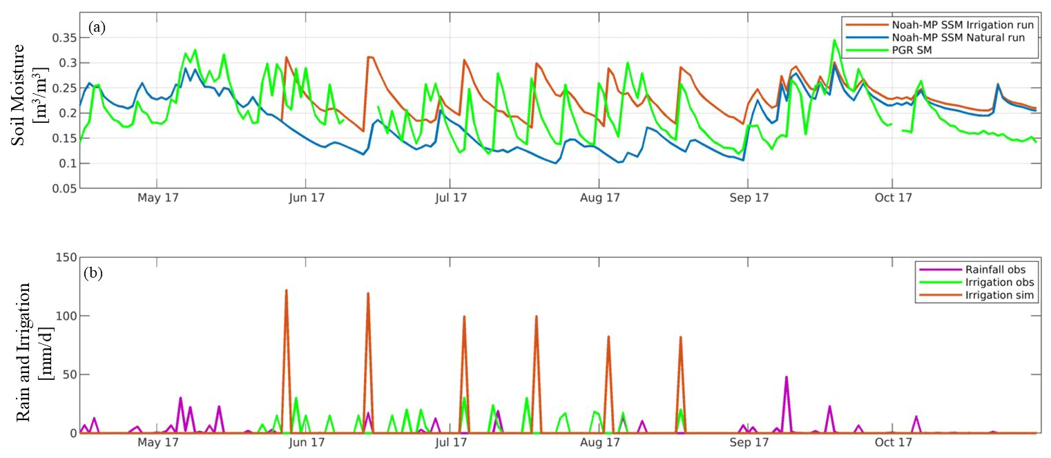
Figure 6(a) Evaluation of SSM over the Budrio field 2, with (green) in situ PGR SM data, (light blue) SSM from Noah-MP natural and (orange) SSM from Noah-MP irrigation. Additional information is provided in panel (b), with observed irrigation (green), simulated irrigation (orange), and observed rainfall (magenta) in millimetres per day (mm d−1).
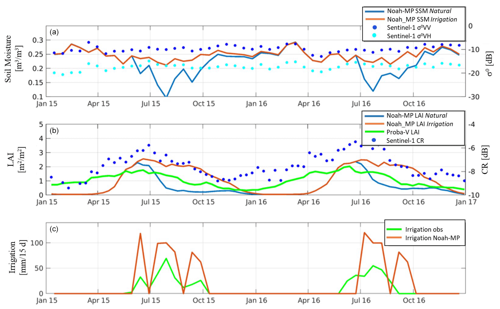
Figure 7Sentinel-1 σ0 VV and σ0 VH data for the Budrio field 1 test site compared with Noah-MP SSM, for (a) natural and irrigation runs. Sentinel-1 CR (VH/VV) compared with PROBA-V LAI and Noah-MP LAI for (b) natural and irrigation runs. Also shown are the (c) observed irrigation (green) and simulated irrigation from Noah-MP (orange).
3.2 Noah MP site evaluation
The Noah-MP SSM was evaluated at the Budrio test site field 2 (Fig. 1a), using the daily reference PGR SM for the year 2017. Comparisons between the SSM simulations of the natural and irrigation runs with in situ PGR SM are shown in Fig. 6a, while daily observed irrigation and rainfall data are compared with daily irrigation simulations in Fig. 6b. Soil moisture data are plotted at their original temporal resolution (i.e. daily) to illustrate an issue related to the irrigation timing, namely that SSM simulations in Fig. 6a show the ability of the sprinkler irrigation scheme to simulate irrigation in the summer season, but there is an inevitable problem in reproducing the correct timing and magnitude of irrigation. Indeed, the total amount of simulated irrigation is 604 mm for the 2017 summer season, which overestimates the total amount of observed irrigation that is 349.5 mm. Furthermore, the model simulations not only miss irrigation but also suffer from erroneous precipitation input, such as on the 11 July 2017, where the observed precipitation event in the growing season is not found in the model SSM simulations. In any case, biweekly Pearson R between simulated SSM and in situ PGR SM are higher for the irrigation run than for the natural run (0.54 vs. 0.42), suggesting the benefit of activating irrigation.
For the Budrio field 1 test site (Fig. 1a), two summer seasons of irrigation data were available. To assess the irrigation information contained in Sentinel-1 σ0 observations (and the potential added value for a forthcoming DA experiment), we compared biweekly values of Sentinel-1 σ0 VV and σ0 VH with SSM estimates from both the natural run and irrigation run (Fig. 7a) for this site. Although the σ0 VV is generally used to retrieve SSM (Wagner et al., 2013; Gruber et al., 2013; Bauer-Marschallinger et al., 2018), data at both polarizations were analysed in order to understand the soil contribution contained in the two signals. Information related to the irrigation periods are shown in Fig. 7c, where irrigation observations and irrigation simulations from Noah-MP are compared. Figure 7a indicates that the SSM simulations are better reflected in the Sentinel-1 σ0 VV than σ0 VH data, particularly when irrigation is simulated (orange line). The SSM estimates from the natural run (light blue line) agree poorly with the Sentinel-1 data, with Pearson R values equal to 0.32 and −0.1 for the σ0 VV (blue dots) and σ0 VH (cyan dots), respectively. When irrigation is simulated, the σ0 VV data better follow the modelled SSM signal (Pearson R of 0.53), especially during the summer irrigation season when the backscatter signal remains higher and stable. On the other hand, σ0 VH seems to provide poor performances, also when irrigation is simulated, with a Pearson R value equal to 0.06, confirming findings by Baghdadi et al. (2017), which highlighted how the use of VH alone to retrieve SSM is suboptimal when vegetation cover is well developed.
In Fig. 7b, the Sentinel-1 σ0 CR (VH/VV) is compared with Noah-MP LAI from the natural run (light-blue line) and irrigation run (orange line). The performance in terms of Pearson R decreases from 0.76 to 0.65 when the irrigation is simulated. This is due to a time shift of the Noah-MP LAI growing season in the irrigation run. PROBA-V LAI (in green) was additionally compared with the Sentinel-1 CR (blue dots), showing a Pearson R of 0.84. The higher agreement between the RS products (Sentinel-1 and PROBA-V) highlights the strong relation between the σ0 CR and the vegetation signal, suggesting a potential benefit of the Sentinel-1 assimilation for correcting the simulated vegetation phenology.
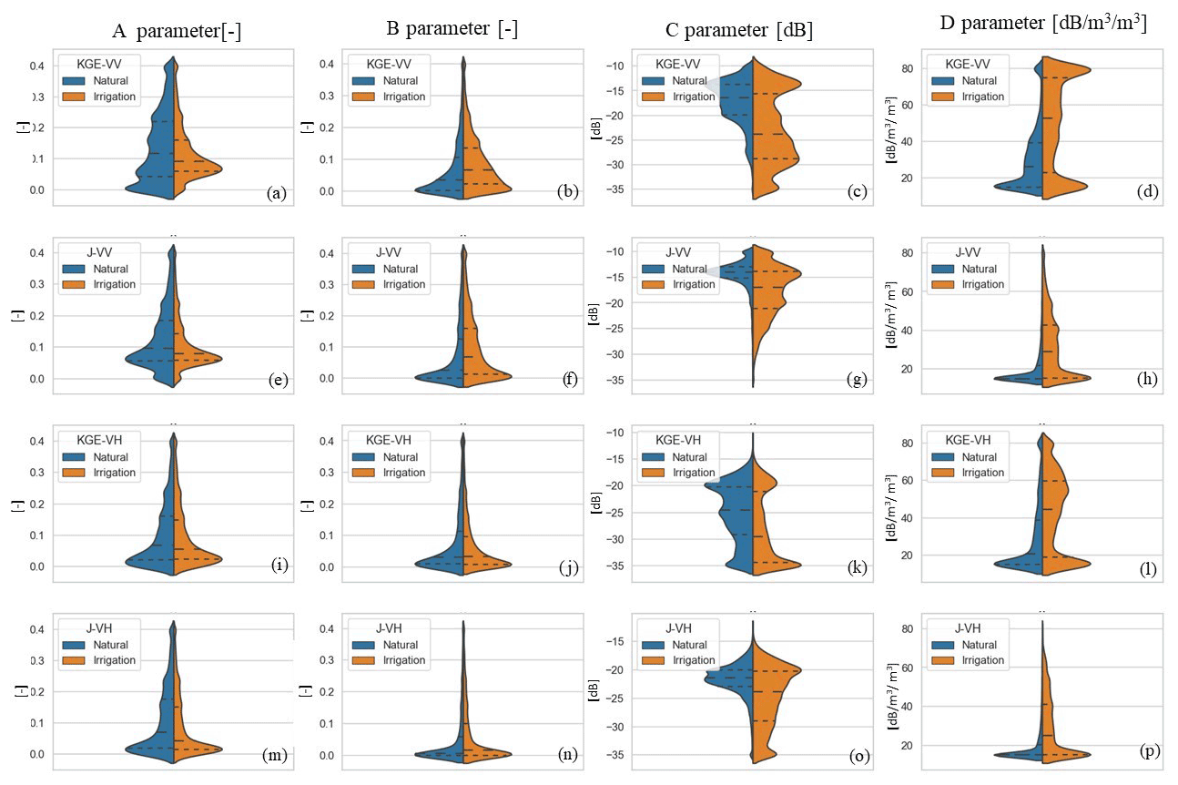
Figure 8Split violin distributions of the calibrated parameters over the entire study area for the eight calibration experiments. For both the natural (blue) and irrigation (orange) experiments, the distributions are shown for the A, B, C, and D parameters, (a–d) using the KGE objective function for VV polarization, (e–h) J objective function for VV polarization, (i–l) KGE objective function for VH polarization, and (m–p) J objective function for VH polarization. Note that the areas under the histograms on both left and right sides of the violins are automatically scaled for optimizing the visualization.
Finally, Fig. 7c shows a comparison between 15 d accumulated millimetres of simulated irrigation (orange) and observed irrigation (green). The Pearson R is equal to 0.77, indicating that the sprinkler irrigation scheme can provide acceptable irrigation estimates at this temporal resolution though absolute irrigation amounts are overestimated.
3.3 WCM calibration
The WCM parameters A and B (vegetation parameters) and C and D (soil parameters) were calibrated for each grid cell separately, during the reference period of January 2017 to December 2019 (Fig. 3), using daily σ0 simulations and observations. The calibrated parameters related to the entire study area for each of the eight experiments are shown in Fig. 8, where the blue (left) parts of the violin plots identify experiments of the natural run, while the orange (right) parts of the violin plots are related to the irrigation run.

Figure 9Maps of the (a) A parameter, (b) B parameter, (c) C parameter, and (d) D parameter for the J-VV natural calibration experiment. Maps of the (e) A parameter, (f) B parameter, (g) C parameter, and (h) D parameter for the J-VV irrigation calibration experiment.
Generally, the J calibration provides parameter distributions closer around their prior guess as compared to the KGE calibration for which the distributions are often multimodal, especially for the C and D parameters (i.e. Fig. 8d and h). This is due to the prior parameter penalty, which is included in the Bayesian solution but not in the KGE. In general, the calibration of the two functions using the natural run provides wider distributions between the lower and upper boundaries for the A vegetation parameter, with a high number of grid cells characterized by A values higher than 0.1 (see KGE-VV natural and J-VV natural experiments in Fig. 8a and e, respectively). Conversely, the irrigation run provides A distributions more skewed to the lower boundary (being also the guess value in each calibration experiment), with a smaller number of grid cells characterized by high A values compared to the natural run. In a preliminary sensitivity study (not shown), we observed that high values of the vegetation parameters A and B, as obtained for the natural run, have the tendency to generate high peaks in the simulated σ0 during the growing season. Indeed, in the summer, the SSM natural signal is low and not consistent with the Sentinel-1 σ0, which observes irrigation. In order to follow the temporal dynamics of the Sentinel-1 σ0, the calibration algorithms attribute a relatively higher weight (higher A values) to the LAI than to SSM to compensate for the underestimated SSM in the natural run. In contrast, the irrigation run provides vegetation parameter distributions more skewed to the lower boundaries (see also Sect. 3.4.2). The C and D parameter distributions feature a better sensitivity to soil moisture dynamics using the irrigation run input data, which is the expected behaviour, considering that they describe the . This is true especially when using the J cost function (see parameters distributions for the J-VV natural and for the J-VV irrigation experiments in Fig. 8g and h), which results in more spread in the calibrated C and D distributions for the irrigation simulations (especially in VV polarization), whereas the mode of the C and D parameter distributions for the natural experiments is more shifted to the upper and lower boundaries, respectively.
Figure 9 shows the spatial pattern of the parameters over the study area to better understand the differences between the natural and irrigation calibration runs. We found a connection between the WCM parameters distribution and model parameters, particularly with the HWSD soil texture map (shown in Fig. 2). For both the J-VV natural and J-VV irrigation experiments, the activation of the irrigation scheme reduces the dependency of the vegetation-related parameters A and B on soil texture (see Fig. 9a and b for the J-VV natural and Fig. 9e and f for the J-VV irrigation experiment). This is also shown in the parameter maps of the KGE calibration experiments (Fig. S5). Additionally, the activation of the irrigation scheme, more realistically, shifts the soil texture dependency towards the soil parameters C and D (Fig. 9g and h), highlighting another important reason for simulating irrigation.
Finally, the different polarization experiments generally provided similar distributions for the vegetation A and B parameters and the D soil parameter. The largest differences between the VV and VH polarizations are identified for the C parameter distributions. This is due to the lower σ0 signal associated with the VH polarization. Indeed, Fig. 8c and g are characterized by higher values of C in the VV polarization, as compared to the distributions for VH polarization in Fig. 8k and o. In the latter, the C–VH distributions are generally more skewed to the lower boundary of the parameters, with median values closer to the defined guess parameter value.
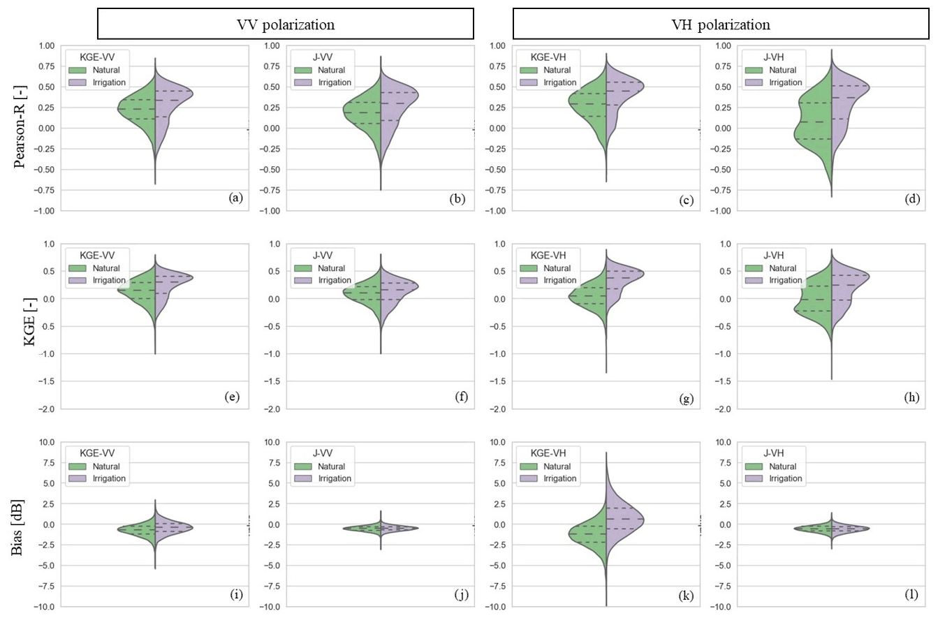
Figure 10Split violin distributions of (a–d) Pearson R, (e–h) KGE, and (i–l) bias calculated between σ0 simulations and observations for the validation period, for all the calibration experiments and considering only the cropland areas, using simulations from the natural run (left; green) and the irrigation run (right; violet). The results are shown for VV (first two columns) and VH (right two columns) and alternate for both the calibration with a J and KGE cost function. Note that the areas under the histograms on both left and right sides of the violins are automatically scaled for optimizing the visualization.
3.4 WCM evaluation
3.4.1 Regional evaluation
The regional evaluation of the calibration experiments was carried out during the period from January 2015 to December 2016 for agricultural areas within the study domain (almost 15 000 km2), by comparing biweekly σ0 simulations with Sentinel-1 σ0 in terms of Pearson R, KGE, and bias. The distribution of the evaluation metrics for the eight experiments is shown in Fig. 10. A comparison of the metrics for the irrigation and natural runs confirms better results when irrigation is activated, with violin plots skewed towards more positive values for both KGE and Pearson R. When stratified by the cost function, the Pearson R distribution in Fig. 10a–d indicates a slightly higher performance for the KGE (Fig. 10a and c) than for J (Fig. 10b and d). In terms of the KGE score, simulations are naturally closer to the observations when the KGE cost function is used. On the other hand, in terms of bias, generally better performances are found when the Bayesian solution is used (Fig. 10i–l). The latter is particularly evident for the VH polarization when comparing the KGE-VH and J-VH experiments (Fig. 10k and l).
The VH simulations exhibit a better performance in the irrigation run than the VV simulations (Fig. 10c and d and 10a and b). Indeed, considering all the statistical scores, the VV polarization is characterized by more similar distributions between the natural and irrigation run for both cost functions. This suggests a higher sensitivity of the VH polarization to the change in vegetation introduced by irrigation, confirming the Sentinel-1 σ0 VH to be strongly influenced by irrigation, as witnessed by the larger score improvement obtained for the calibration experiments KGE-VH irrigation (Fig. 10g) and J-VH irrigation (Fig. 10h) when compared to the natural run experiments.
In summary, (i) VH polarization is more sensitive to the change in the cost function and input data (irrigation or natural run) than VV polarization, likely due to its higher sensitivity to vegetation change (Vreugdenhil et al., 2018; Macelloni et al. 2001), which, in the area, is related to the crop development after irrigation, and (ii) the combination of J with the activation of the irrigation scheme is able to provide the best unbiased estimates of simulated σ0 for both VV and VH (J-VV irrigation and J-VH irrigation experiments) at the price of generally lower correlations (compared to the KGE cost function). This is, however, beneficial for DA as it minimizes the chance of potential error cross-correlation between model estimates and observations. Indeed, the match of the temporal dynamic of the signals induced by the correlation term is stronger in the KGE than in J, which, additionally, includes a parameter constraint. The higher weight of the correlation in the KGE cost function can negatively impact the parameter calibration, even when irrigation is turned on in Noah-MP, because the simulated irrigation applications are, in general, not temporally consistent with those seen by Sentinel-1 (see Fig. 6).
Table 2Results of the site WCM evaluation considering the test site Faenza San Silvestro for each WCM experiment.


Figure 11Comparisons between σ0 observations (VV polarization in blue dots and VH polarization light blue dots) and simulations (VV polarization in red and VH polarization in green) in the Faenza (San Silvestro) field, after calibration with a KGE cost function for (a) the natural run, (b) the irrigation run, and after calibration with the J cost function for (c) the natural and (d) irrigation runs.
3.4.2 In situ evaluation
The WCM simulations are further analysed in detail at the Faenza test site (specifically for the San Silvestro field) because it has a larger extent than the Budrio site (see Fig. 1), although the same overall conclusions were found for Budrio. Figure 11 shows the simulated and observed σ0 time series for the different experiments highlighted in Fig. 3, and Table 2 summarizes the statistics (i.e. Pearson R, KGE and bias) of each experiment.
The agreement between simulated and observed σ0 measured by the Pearson R and KGE in Table 2 generally gives better performances after calibration with the KGE cost function than with the J cost function. An example is in the higher correlations found for the KGE-VH irrigation experiment as compared to the J-VH irrigation (Fig. 11b and d, respectively). On the other hand, in terms of bias, the cost function J significantly outperforms the calibration with KGE in all experiments with surprisingly comparable values between natural and irrigation runs (Table 2).
One undesirable feature of natural runs is the presence of high σ0 peaks during the summer, clearly detectable over the Faenza test site, especially in the VH polarization, which are less evident in the irrigation run (see Fig. 11b and d). A similar behaviour was found for Budrio (not shown). These peaks are likely attributed to the poor estimation of model vegetation parameter values, previously discussed in Sect. 3.3, when the WCM attempts to compensate for bias in SSM and vegetation input, i.e. input that is not consistent with observations over irrigated areas. This is particularly true for the KGE calibration, which does not use a prior parameter constraint. In contrast, the J calibration still provides reasonable σ0 simulations that are closer to the ones of the irrigation run due to the Bayesian technique itself.
4.1 Noah-MP irrigation modelling
The Noah-MP LSM, used as input for the WCM calibration, was evaluated in two configurations, either with a sprinkler irrigation scheme activated or without irrigation (i.e. irrigation run and natural run). Although not all of the Po Valley is irrigated by sprinkler systems, it most likely still leads to more realistic LSM simulations than not considering irrigation at all.
The main limitation found in the irrigation simulations was related to the irrigation timing and magnitude that was inconsistent with observations. Although this finding is based on only a single study site, it is very likely that it is a widespread issue within the study area for several reasons. In LSMs, the irrigation application is driven by the RZSM availability and, consequently, by the soil type and the rooting depth parameterizations. Moreover, it is also influenced by the accuracy of the meteorological forcings (especially precipitation), which can determine errors in the soil moisture representation. The main reason, however, is likely that irrigation is often the result of subjective farmer decisions rather than objective rules based on the soil state and crop conditions. In theory, the irrigation timing issue could be partly solved by using temporally consistent high-resolution crop maps, which should provide a more realistic information of crop phenology and rooting depth. However, in practice, this is unfeasible over many areas of the world given the absence of this information on a large scale. Also, given that irrigation applications are mainly linked to unmodelled processes, like rotation schedules for farmers to withdraw water, the correct simulation of the timing can be unsolvable when using models only.
Despite the potential problems related to the unrealistic assumptions in the simulation of irrigation, our results demonstrated that even the use of simple irrigation schemes within Noah-MP can be beneficial. In the regional evaluation, SSM simulations of the natural and irrigation runs were compared with RS SSM from SMAP and ASCAT (Fig. 4) on a biweekly temporal scale. For both products, we found large improvements in temporal Pearson R when irrigation was simulated, which were confirmed by a decrease in the RMSE values over croplands, suggesting that the activation of irrigation modelling provides more realistic SSM estimates. Our findings further confirm the potential of coarse-resolution data sets for providing irrigation-related information over intensively irrigated and relatively large agricultural areas, as was shown by S. V. Kumar et al. (2015).
While the impact of irrigation was clear in terms of SSM, the regional evaluation of the simulated LAI against the PROBA-V-based LAI provided contradicting results. In this case, the Pearson R analysis suggested a deterioration of the Noah-MP-simulated LAI when irrigation was activated over the cropland area. We interpreted this correlation deterioration from the absence of specific information about the crop phenology in the model parameterization. In practice, information about the specific crop type is not available, and the rooting depth is the sole parameter controlling water uptake from the soil layers. Additionally, information on sowing and harvest periods are not included in the current version of Noah-MP, while irrigated areas are defined based on a global data set (Salmon et al., 2015) which can suffer accuracy limitations. Indeed, the absence of annual dynamic information on irrigated fields, the unknown yearly variability of the crop types, and the impact of the meteorological conditions in the stakeholders' decision-making process (i.e. sowing) make the simulation of Noah-MP prone to LAI peak shifts, as compared to observations, when irrigation is simulated. Another important aspect affecting LAI simulations is its sensitivity to root zone soil moisture, which might be more difficult to simulate than SSM during the irrigation season due to larger impacts of the soil texture and transpiration processes along with the high frequency of the wetting and drying phases caused by irrigation events. This results in a significant performance deterioration (often worse than LAI simulations not including irrigation which are mainly driven by seasonality; see Fig. 7). In contrast, irrigation modeling helps to reduce the bias of the LAI-simulated time series, which, in the cropland area, show a significant underestimation when irrigation is not considered.
The limitations found in simulating LAI and vegetation by Noah-MP, even when irrigation was simulated, could potentially be overcome by assimilating Sentinel-1 σ0 data. To explore this potential, we compared the LAI from both model runs, and from PROBA-V, with the observed Sentinel-1 σ0 CR (VH/VV), which should provide information about the vegetation dynamics (Vreugdenhil et al., 2018, 2020). We found that the correlation between σ0 CR and LAI from PROBA-V was much higher than that between σ0 CR and the simulated LAI by Noah-MP (see Fig. 7), suggesting that Sentinel-1 σ0 DA could help to correct poor LAI model simulations. Additionally, a higher correlation was found between the σ0 VV observations and the simulated SSM when irrigation was turned on than in the absence of irrigation, suggesting that the assimilation of σ0 VV could improve SSM where irrigation is poorly modelled or not modelled. On the other hand, considering the low correlation between the VH signal and SSM in presence of vegetation (Baghdadi et al. 2017), and its close relation with vegetation (Ferrazzoli et al., 1992; Macelloni et al., 2001), future data assimilation experiments will investigate the contribution of VH and CR in improving LAI predictions and irrigation quantification.
Finally, biweekly accumulated irrigation estimates in Fig. 7 agree well with real irrigation applications, suggesting that the large-scale LSM irrigation scheme is helpful for intensively irrigated areas. On the other hand, the poor soil and crop parameterization, along with other unknown parameters related to the irrigation management (e.g. the farmers can apply more water than actually needed), can cause large biases in these irrigation simulations. Again, ingestion of radar backscatter data could correct for unmodelled processes. More specifically, Sentinel-1 σ0 could correct (i) for the magnitude and timing of the irrigation simulations and (ii) for Noah-MP irrigation predictions over regions that are not irrigated.
4.2 WCM backscatter simulation
The purpose of the presented WCM observation operator calibration and evaluation was to optimize the parameters for the future assimilation of the Sentinel-1 σ0 VV and VH into Noah-MP. Such an optimization would ideally minimize the long-term bias between the simulated and observed σ0 signals. This can be achieved by calibrating the observation operator with long-term observed σ0 prior to data assimilation, but in this process, it is crucial to avoid potential error cross-correlation between model observation predictions and observations. Furthermore, a good observation operator should not already compensate for missing processes in the LSM by accepting effective, but unrealistic, optimized parameters because it would then lose its physically based ability to accurately convert misfits between observations and simulations to LSM updates during the data assimilation.
One way to avoid parameters compensating for erroneous LSM input into the WCM would be to use observed time series of, e.g., LAI. However, LAI products from different sensors have different biases themselves, which can add bias to the σ0 simulations, and more importantly, replacing simulated LAI or SSM with external data sets would undermine the possibility of updating these variables in the future assimilation system. Based on that, we performed the WCM calibration considering the SSM and LAI model input from two different experiments, i.e. a natural run and an irrigation run, as well as two cost functions, a Bayesian solution J, and a KGE solution, which resulted in four calibration experiments for each polarization (i.e. eight calibration experiments in total).
The calibration experiments using simulations from the natural run as input showed a limited performance and provided presumably bad vegetation parameter estimates, which resulted in unrealistic peaks in the simulated σ0 during the summer when driven by higher modelled LAI during this period. The inclusion of the irrigation within Noah-MP was very beneficial for all the calibration experiments, helping to reduce the bias, increase the correlation with Sentinel-1 σ0, and remove the anomalous σ0 increase during warm periods, especially for the KGE-based calibration. This corroborates our initial hypothesis that, over intensively irrigated areas, the simulation of irrigation is a mandatory task for an optimal calibration of the WCM. Irrigation modeling, even if only done approximately and perhaps with inaccurate timing, reduces obvious land surface (soil moisture and vegetation) bias and avoids that the WCM needs to compensate for this bias.
Our results show overall higher performance in terms of KGE and Pearson R scores for the KGE-based calibration, whereas the long-term bias was better reduced for the J-based calibration, which is beneficial in anticipation of future DA. This is because, in the J cost function, there is (i) a target accuracy term which also takes into account the Sentinel-1 observations, where an error is present, and (ii) a parameter deviation penalty based on the prior parameters constraints is used, which prevents parameters from deviating largely from their prior values.
In terms of polarization, we found σ0 VH simulations much more sensitive to the inclusion of the irrigation (vs. non-inclusion) in Noah-MP, suggesting that observed σ0 VH might also contain much more information about irrigation (via the influence of the vegetation change due to irrigation) than that contained in σ0 VV, which is normally used for SSM retrieval (Vreugdenhil et al., 2020). We believe that the cause of this is related to a comparatively larger σ0 of vegetation with respect to that of the soil when the crops are well developed. This was also corroborated by the better agreement between CR and LAI from PROBA-V in one of the study sites mentioned above. Despite this, further investigations are required to confirm this hypothesis, and DA will certainly help to test this aspect.
With the specific focus on intensively irrigated land, the main objective of this work was to define the optimal calibration of the WCM as an observation operator for the future ingestion of Sentinel-1 backscatter into the Noah-MP LSM via DA. In this context, we additionally aimed at (1) unveiling the strengths and limitations of irrigation simulation in LSMs from the perspective of a calibrating the WCM and (2) identifying the potential irrigation-related information contained in the Sentinel-1 σ0 observations to improve soil moisture and vegetation states, as well as irrigation estimates, in a calibrated DA system.
To reach these objectives, we coupled the Noah-MP with a sprinkler irrigation scheme within LIS and performed two different simulation experiments, i.e. one with and one without irrigation (i.e. natural and irrigation runs). Moreover, we coupled a WCM with Noah-MP and tested different calibration options to prepare for the optimal, future, assimilation of σ0 VV and VH to update both soil moisture and vegetation states.
The main conclusions drawn from our evaluation are as follows:
-
Over highly irrigated areas, the simulation of irrigation in LSMs helps to provide better soil moisture and vegetation simulations, which can be used with benefit as input for the WCM calibration. However, the performance of the irrigation simulations is limited by the simplistic model parameterization of this human process and the necessity for considering realistic and updated land cover information (e.g. crop types). This results in poor simulations of the irrigation timing and quantities, as well as vegetation dynamics.
-
The Sentinel-1 σ0 observations contain useful information about SSM and vegetation over highly irrigated areas. This information can be exploited to overcome LSM deficiencies in simulating soil moisture and vegetation over highly irrigated regions, e.g. when irrigation is unmodelled or poorly modelled because of uncertainties due to crop types, irrigation timing, and farmer agricultural practices. In particular, there is a high chance that the assimilation of Sentinel-1 σ0 can help in correcting LAI dynamics.
-
The optimal assimilation of Sentinel-1 σ0 into a LSM must rely upon a well-calibrated WCM as the observation operator to provide unbiased σ0 simulations with a minimal chance of having error cross-correlations between model and observations, while ensuring a realistic operator controllability or realistic connection between observed signals and land surface state variables. We demonstrated that calibrating the WCM by including irrigation modeling consistently led to a better agreement with Sentinel-1 σ0. The modeling of irrigation in the LSM simulations, even if not done optimally, avoids that the WCM calibration compensates for LSM biases.
-
We demonstrated that the WCM calibration with a Bayesian cost function, including a prior parameter constraint, provides the optimal WCM parameters, is able to generate the lowest bias in the σ0 simulations for both VV and VH. Although slightly higher correlations are obtained when using a KGE cost function, unbiased estimates are particularly beneficial for DA, as this minimizes the chance of potential error cross-correlation between model estimates and observations.
This study improves the understanding of the LSM limitations in simulating irrigation and highlights the information content in Sentinel-1 σ0 data. A natural follow-up of this study is the assimilation of σ0 observations within Noah-MP, which should enforce our tested evidence and provide new insights for a more realistic description of the water and carbon cycles over irrigated areas.
Data from SMAP can be downloaded at https://doi.org/10.5067/Q8J8E3A89923 (O'Neill et al., 2020). Data from ASCAT are available from the website https://www.cen.uni-hamburg.de/en/icdc/data/land/docs-land/h115-ascat-ssm-cdr-v5-pum-v0-1.pdf (EUMETSAT, 2019). The Sentinel-1 backscatter data processing was done using Google Earth Engine's Python interface and including standard processing techniques. Data from PROBA-V are available at https://land.copernicus.vgt.vito.be/PDF/portal/Application.html#Browse;Root=512260;Collection=1000083;Time=NORMAL,NORMAL,-1,,,-1,, (Verger et al., 2014). MERRA-2 data are available from MDISC, which is managed by the NASA Goddard Earth Sciences (GES) Data and Information Services Center (DISC; https://disc.gsfc.nasa.gov/datasets?project=MERRA-2; Gelaro et al., 2017). The LIS source code and default input parameters are available via https://lis.gsfc.nasa.gov/ (Kumar, 2021). The 100 m spatial resolution land cover map from the Copernicus Global Land Service can be downloaded from https://lcviewer.vito.be/2015 (Buchhorn et al., 2020). In situ data are available upon request to the original providers. The ETOPO1 1 arcmin global relief model used in Fig. 1 can be downloaded at https://doi.org/10.7289/V5C8276M (Amante and Eakins, 2009).
The supplement related to this article is available online at: https://doi.org/10.5194/hess-25-6283-2021-supplement.
SM designed and coordinated the study and did the analyses. CM, GJMDL, and AG designed, coordinated, and helped with the data analysis and interpretation. HL, AT, and RM helped with the result interpretation and data processing and collection. All authors contributed to the editing of the paper.
The contact author has declared that neither they nor their co-authors have any competing interests.
Publisher's note: Copernicus Publications remains neutral with regard to jurisdictional claims in published maps and institutional affiliations.
The authors would like to thank the European Space Agency (ESA) for funding support as part of the IRRIGATION+ project. For details, please visit https://esairrigationplus.org/ (last access: 2 December 2021). Additional acknowledgements go to the Canale Emiliano Romagnolo (CER; Emilia Romagna, Italy), for providing irrigation data over the irrigated test sites. For the Proximal Gamma Ray soil moisture data at the Budrio test site, the authors would like to thank the Department of Physics and Earth Sciences, University of Ferrara Polo Scientifico e Tecnologico, and, in particular, Martina Natali, Virginia Strati, Alberi Matteo, Kassandra Giulia Raptis, and Fabio Mantovani. Additionally, the authors want to acknowledge Kristi Arsenault from NASA Goddard Space Flight Center (GFSC) for sharing important technical information on irrigation simulations into the Land Information System (LIS) framework and the Vlaams Supercomputer Centrum (VSC) high-performance computing (HPC) for providing the computational resources needed to realize this study (https://www.vscentrum.be/, last access: 2 December 2021). Alexander Gruber has received funding from the Research Foundation Flanders.
This research has been supported by the European Space Agency (ESA) as part of the IRRIGATION+ project (contract no. 4000129870/20/I-NB). Alexander Gruber has been supported by the Research Foundation Flanders (grant no. FWO-1224320N).
This paper was edited by Louise Slater and reviewed by two anonymous referees.
Albergel, C., Munier, S., Bocher, A., Bonan, B., Zheng, Y., Draper, C., Leroux, D. J., and Calvet, J.-C.: LDAS-Monde Sequential Assimilation of Satellite Derived Observations Applied to the Contiguous US: An ERA-5 Driven Reanalysis of the Land Surface Variables, Remote Sens.-Basel, 10, 1627, https://doi.org/10.3390/rs10101627, 2018.
Amante, C. and Eakins, B. W.: ETOPO1 1 Arc-Minute Global Relief Model: Procedures, Data Sources and Analysis, 685 NOAA Technical Memorandum NESDIS NGDC-24, National Geophysical Data Center, NOAA [data set], https://doi.org/10.7289/V5C8276M, 2009.
Ambika, A. K., Wardlow, B., and Mishra, V.: Remotely sensed high resolution irrigated area mapping in India for 2000 to 2015, Sci. Data, 3, 160118, https://doi.org/10.1038/sdata.2016.118, 2016.
Arsenault, K. R., Kumar, S. V., Geiger, J. V., Wang, S., Kemp, E., Mocko, D. M., Beaudoing, H. K., Getirana, A., Navari, M., Li, B., Jacob, J., Wegiel, J., and Peters-Lidard, C. D.: The Land surface Data Toolkit (LDT v7.2) – a data fusion environment for land data assimilation systems, Geosci. Model Dev., 11, 3605–3621, https://doi.org/10.5194/gmd-11-3605-2018, 2018.
Attema, E. P. W. and Ulaby, F. T.: Vegetation modelled as a water cloud, Radio Sci., 13, 357–364, https://doi.org/10.1029/RS013i002p00357, 1978.
Badger, A. M. and Dirmeyer, P. A.: Climate response to Amazon forest replacement by heterogeneous crop cover, Hydrol. Earth Syst. Sci., 19, 4547–4557, https://doi.org/10.5194/hess-19-4547-2015, 2015.
Baghdadi, N., Hajj, M. E., Zribi, M., and Bousbih, S.: Calibration of the water cloud model at C-band for winter crop fields and grasslands, Remote Sens.-Basel, 9, 969, https://doi.org/10.3390/rs9090969, 2017.
Bai, X. and He, B.: Potential of Dubois model for soil moisture retrieval in prairie areas using SAR and optical data, Int. J. Remote Sens., 36, 5737–5753, https://doi.org/10.1080/01431161.2015.1103920, 2015.
Baldoncini, M., Alberi, M., Bottardi, C., Chiarelli, E., Raptis, K. G. C., Strati, V., and Mantovani, F.: Biomass water content effect on soil moisture assessment via proximal gamma-ray spectroscopy, Geoderma, 335, 69–77, https://doi.org/10.1016/j.geoderma.2018.08.012, 2019.
Ball, J. T., Woodrow, I. E., and Berry, J. A.: A model predicting stomatal conductance and its contribution to the control of photosynthesis under different environmental conditions, in: Process in Photosynthesis Research, Vol. 1, edited by: Biggins, J., Martinus Nijhoff, Dordrecht, the Netherlands, 221–234, 1987.
Bauer-Marschallinger, B., Freeman, V., Cao, S., Paulik, C., Schaufler, S., Stachl, T., Modanesi, S., Massari, C., Ciabatta, L., Brocca, L., and Wagner, W.: Toward Global Soil Moisture Monitoring With Sentinel-1: Harnessing Assets and Overcoming Obstacles, IEEE T. Geosci. Remote, 57, 520–539, https://doi.org/10.1109/TGRS.2018.2858004, 2018.
Bazzi, H., Baghdadi, N., Ienco, D., ElHajj, M., Zribi, M., Belhouchette, H., Escorihuela, M. J., and Demarez, V.: Mapping Irrigated Areas Using Sentinel-1 Time Series in Catalonia, Spain, Remote Sens.-Basel, 11, 1836, https://doi.org/10.3390/rs11151836, 2019.
Buchhorn, M., Lesiv, M., Tsendbazar, N. E., Herold, M., Bertels, L., and Smets, B.: Copernicus global land cover layers – collection 2, Remote Sens., 12, 1044, https://doi.org/10.3390/rs12061044, 2020 (data available at: https://lcviewer.vito.be/2015, last access: 7 December 2021).
Girotto, M., De Lannoy, G. J., Reichle, R. H., Rodell, M., Draper, C., Bhanja, S. N., and Mukherjee, A.: Benefits and pitfalls of GRACE data assimilation: A case study of terrestrial water storage depletion in India, Geophys. Res. Lett., 44, 4107–4115, https://doi.org/10.1002/2017GL072994, 2017.
Bousbih, S., Zribi, M., El Hajj, M., Baghdadi, N., Lili-Chabaane, Z., Gao, Q., and Fanise, P.: Soil moisture and irrigation mapping in a semi-arid region based on the synergic use of Sentinel-1 and Sentinel-2 data, Remote Sens., 10, 1953, https://doi.org/10.3390/rs10121953, 2018.
Breña-Naranjo, J. A., Kendall, A. D., and Hyndman, D. W.: Improved methods for satellite-based groundwater storage estimates: A decade of monitoring the high plains aquifer from space and ground observations, Geophys. Res. Lett., 41, 6167–6173, https://doi.org/10.1002/2014GL061213, 2014.
Bretreger, D., Yeo, I.-Y., Hancock, G., and Willgoose, G.: Monitoring irrigation using landsat observations and climate data over regional scales in the Murray–Darling Basin, J Hydrol., 590, 125356, https://doi.org/10.1016/j.jhydrol.2020.125356, 2020.
Brocca, L., Ciabatta, L., Massari, C., Moramarco, T., Hahn, S., Hasenauer, S., Kidd, R., Dorigo, W., Wagner, W., and Levizzani, V.: Soil as a natural rain gauge: estimating global rainfall from satellite soil moisture data, J. Geophys. Res., 119, 5128–5141, https://doi.org/10.1002/2014JD021489, 2014.
Brocca, L., Tarpanelli, A., Filippucci, P., Dorigo, W., Zaussinger, F., Gruber, A., and Fernández-Prieto, D.: How much water is used for irrigation? A new approach exploiting coarse resolution satellite soil moisture products, Int. J. Appl. Earth Obs., 73C, 752–766, https://doi.org/10.1016/j.jag.2018.08.023, 2018.
Brodzik, M., Billingsley, B., Haran, T., Raup, B., and Savoie, M.: EASE-Grid 2.0: Incremental but Significant Improvements for Earth-Gridded Data Sets, ISPRS Int. J. Geo-Inf., 1, 32–45, https://doi.org/10.3390/ijgi1010032, 2012.
Carrera, M. L., Bilodeau, B., Bélair, S., Abrahamowicz, M., Russell, A., and Wang, X.: Assimilation of passive L-band microwave brightness temperatures in the Canadian Land Data Assimilation System: Impacts on short-range warm season numerical weather prediction, J. Hydrometeorol., 20, 1053–1079, https://doi.org/10.1175/JHM-D-18-0133.1, 2019.
Chan, S., Bindlish, R., O'Neill, P. E., Jackson, T., Njoku, E. G., Dunbar, S., Chaubell, J., Piepmeier, J. R., Yueh, S., Entekhabi, D., Colliander, A., Chen, F., Cosh, M., Caldwell, T., Walker, J., Berg, A., McNairn, H., Thibeault, M., Martinez-Fernandez, J., Uldall, F., Seyfried, M., Bosch, D., Starks, P., Collins, C. H., Prueger, J., Van der Velde, R., Asanuma, J., Palecki, M., Small, E. E., Zreda, M., Calvet, J., Crow, W. T., and Kerr, Y.: Development and assessment of the SMAP enhanced passive soil moisture product, Remote Sens. Environ., 204, 931–941, https://doi.org/10.1016/j.rse.2017.08.025, 2018.
Chen, F. and Dudhia, J.: Coupling an advanced land surface hydrology model with the Penn State-NCAR MM5 modeling system. Part I: Model implementation and sensitivity, Mon. Weather Rev., 129, 569–585, https://doi.org/10.1175/1520-0493(2001)129<0569:CAALSH>2.0.CO;2, 2001.
Chen, F., Mitchell, K., Schaake, J., Xue, Y., Pan, H. L., Koren, V., Duan, Q. Y., Ek, M., and Betts, A.: Modeling of land surface evaporation by four schemes and comparison with fife observations, J. Geophys. Res.-Atmos., 101, 7251–7268, https://doi.org/10.1029/95JD02165, 1996.
Copernicus Global Land Service Site: available at: https://land.copernicus.eu/global/, last access: 30 November 2021.
Dari, J., Brocca, L., Quintana-Seguí, P., Escorihuela, M. J., Stefan, V., and Morbidelli, R.: Exploiting High-Resolution Remote Sensing Soil Moisture to Estimate Irrigation Water Amounts over a Mediterranean Region, Remote Sens.-Basel, 12, 2593, https://doi.org/10.3390/rs12162593, 2020.
De Lannoy, G. J. M., Reichle, R., and Pauwels, V.: Global calibration of the GEOS-5 L-band microwave radiative transfer model over non-frozen land using SMOS observations, J. Hydrometeorol., 14, 765–785, https://doi.org/10.1175/JHM-D-12-092, 2013.
De Lannoy, G. J. M., Reichle, R. H., and Vrugt, J. A.: Uncertainty quantification of GEOS-5 L-band radiative transfer model parameters using Bayesian inference and SMOS observations, Remote Sens. Environ., 148, 146–157, https://doi.org/10.1016/j.rse.2014.03.030, 2014.
De Lannoy, G. J. M. and Reichle, R. H.: Assimilation of SMOS brightness temperatures or soil moisture retrievals into a land surface model, Hydrol. Earth Syst. Sci., 20, 4895–4911, https://doi.org/10.5194/hess-20-4895-2016, 2016.
Dierckx, W., Sterckx, S., Benhadj, I., Livens, S., Duhoux, G.,Van Achteren, T., Francois, M., Mellab, K., and Saint, G.: PROBA-V mission for global vegetation monitoring: Standard products and image quality, Int. J. Remote Sens., 35, 2589–2614, https://doi.org/10.1080/01431161.2014.883097, 2014.
Douglas, E., Beltran-Przekurat, A., Niyogi, D., Pielke Sr, R., and Vörösmarty, C. J.: The impact of agricultural intensification and irrigation on land–atmosphere interactions and Indian monsoon precipitation – A mesoscale modeling perspective, Glob. Planet. Change, 67, 117–128, https://doi.org/10.1016/j.gloplacha.2008.12.007, 2009.
EC: Council Directive 2000/60/EC of 23. October 2000 establishing a framework for community action in the field of water policy Off. J. Eur. Communities, L 327, 1–72, 2000.
Ek, M. B., Mitchell, K. E., Lin, Y., Rogers, E., Grunmann, P., Koren, V., Gayno, G., and Tarpley, J. D.: Implementation of Noah land surface model advancements in the National Centers for Environmental Prediction operational mesoscale Eta model, J. Geophys. Res., 108, 8851, https://doi.org/10.1029/2002JD003296, 2003.
El Hajj, M., Baghdadi, N., Zribi, M., Belaud, G., Cheviron, B., Courault, D., and Charron, F: Soil moisture retrieval over irrigated grassland using X-band SAR data, Remote Sens. Environ., 176, 202–218, https://doi.org/10.1016/j.rse.2016.01.027, 2016.
El Hajj, M., Baghdadi, N., Zribi, M., and Bazzi, H.: Synergic Use of Sentinel-1 and Sentinel-2 Images for Operational Soil Moisture Mapping at High Spatial Resolution over Agricultural Areas, Remote Sens.-Basel, 9, 1292, https://doi.org/10.3390/rs9121292, 2017.
Entekhabi, D., Njoku, E. G., O'Neill, P. E., Kellogg, K. H., Crow, W. T., Edelstein, W. N., Entin, J. K., Goodman S. D., Jackson, T. J., Johnson, T. J., Kimball, J., Piepmeier, J. R., Koster, R. D., Martin, N., McDonald, K. C., Moghaddam, M., Moran, S., Reichle R., Shi, J. C., Spencer. M. W., Thurman, S. W., Tsang, L., and Van Zyl, J.: The Soil Moisture Active and Passive (SMAP) mission, Proceedings of the IEEE, 98, 704–716, https://doi.org/10.1109/JPROC.2010.2043918, 2010.
Escorihuela, M. J. and Quintana-Segui, P.: Comparison of remote sensing and simulated soil moisture datasets in Mediterranean landscapes, Remote Sens. Environ., 180, 99–114, https://doi.org/10.1016/j.rse.2016.02.046, 2016.
EUMETSAT: Product User Manual (PUM) Metop ASCAT soil moisture climate data record v5 12.5 km (H115) and extension (H116), In EUMETSAT Satellite application facility on support to operational hydrology and water management Doc. SAF/HSAF/CDOP3/PUM, p. 32, available at: https://www.cen.uni-hamburg.de/en/icdc/data/land/docs-land/h115-ascat-ssm-cdr-v5-pum-v0-1.pdf (last access: 7 December 2021), 2019.
Evans, J. P. and Zaitchik, B. F.: Modeling the large-scale water balance impact of different irrigation systems, Water Resour. Res., 44, W08448, https://doi.org/10.1029/2007WR006671, 2008.
FAO: The FAO-Unesco Soil Map of the World, Legend and 9 volumes, Unesco, Paris, France, 1971.
FAO: AQUASTAT online database, available at: http://www.fao.org/ag/agl/aglw/aquastat/main/index.stm (last access: 30 November 2021), Food and Agriculture Organization of the United Nations (FAO), 2006.
Ferrazzoli, P., Paloscia, S., Pampaloni, P., Schiavon, G., Solimini, D., and Coppo, P.: Sensitivity of microwave measurements to vegetation biomass and soil moisture content: A case study, IEEE T. Geosci. Remote, 30, 750–756, https://doi.org/10.1109/36.158869, 1992.
Filippucci, P., Tarpanelli, A., Massari, C., Serafini, A., Strati, V., Alberi, M., Raptis, K. G. C., Mantovani, F., and Brocca, L.: Soil moisture as a potential variable for tracking and quantifying irrigation: A case study with proximal gamma-ray spectroscopy data, Adv. Water Resour., 136, 103502, https://doi.org/10.1016/j.advwatres.2019.103502, 2020.
Foley, J. A., Ramankutty, N., Brauman, K. A., Cassidy, E. S., Gerber, J. S., Johnston, M., and Balzer, C.: Solutions for a cultivated planet, Nature, 478, 337–342, https://doi.org/10.1038/nature10452, 2011.
Foster, T., Mieno, T., and Brozovic, N.: Satellite-based monitoring of irrigation water use: Assessing measurement errors and their implications for agricultural water management policy, Water Resour. Res., 56, e2020WR028378, https://doi.org/10.1029/2020WR028378, 2020.
Francois, M., Santandrea, S., Mellab, K., Vrancken, D., and Versluys, J.: The PROBA-V mission: The space segment, Int. J. Remote Sens., 35, 2548–2564, https://doi.org/10.1080/01431161.2014.883098, 2014.
Fung, A.: Microwave Scattering and Emission Models and their Applications, Artech House, Boston, MA, 1994.
Gao, Q., Zribi, M., Escorihuela, M., Baghdadi, N., and Segui, P.: Irrigation mapping using Sentinel-1 time series at field scale, Remote Sens.-Basel, 10, 1495, https://doi.org/10.3390/rs10091495, 2018.
Gelaro, R., McCarty, W., Suárez, M. J., Todling, R., Molod, A., Takacs, L., Randles, C. A., Darmenov, A., Bosilovich, M. G., Reichle, R., Wargan, K., Coy, L., Cullather, R., Draper, C., Akella, S., Buchard, V., Conaty, A., da Silva, A. M., Gu, W., Kim, G.-K., Koster, R., Lucchesi, R., Merkova, D., Nielsen, J. E., Partyka, G., Pawson, S., Putman, W., Rienecker, M., Schubert, S. D., Sienkiewicz, M., and Zhao, B.: The modern-era retrospective analysis for research and applications, version 2 (MERRA-2), J. Climate, 30, 5419–5454, https://doi.org/10.1175/JCLI-D-16-0758.1, 2017 (data available at: https://disc.gsfc.nasa.gov/datasets?project=MERRA-2, last access: 20 May 2021).
Gruber, A., Wagner, W., Hegyiova, A., Greifeneder, F., and Schlaffer, S.: Potential of Sentinel-1 for high-resolution soil moisture monitoring, in: 2013 IEEE International Geoscience and Remote Sensing Symposium-IGARSS, 4030–4033, 2013.
Gupta, H. V., Kling, H., Yilmaz, K. K., and Martinez, G. F.: Decomposition of the mean squared error and NSE performance criteria: implications for improving hydrological modelling, J. Hydrol., 377, 80–91, https://doi.org/10.1016/j.jhydrol.2009.08.003, 2009.
Gutman, G. and Ignatov, A.: The derivation of the green vegetation fraction from NOAA/AVHRR data for use in numerical weather prediction 720 models, Int. J. Remote Sens., 19, 1533–1543, https://doi.org/10.1080/014311698215333, 1998.
H SAF: Algorithm Theoretical Baseline Document (ATBD) Metop ASCAT Surface Soil Moisture Climate Data Record v5 12.5 km sampling (H115) and Extension (H116), v0.1, available at: http://hsaf.meteoam.it/ (last access: 20 May 2021), 2019.
Haddeland, I., Skaugen, T., and Lettenmaier, D. P.: Hydrologic effects of land and water management in North America and Asia: 1700–1992, Hydrol. Earth Syst. Sci., 11, 1035–1045, https://doi.org/10.5194/hess-11-1035-2007, 2007.
Hansen, M. C., DeFries, R. S., Townshend, J. R., and Sohlberg, R.: Global land cover classification at 1 km spatial resolution using a classification tree approach, Int. J. Remote Sens., 21, 1331–1364, https://doi.org/10.1080/014311600210209, 2000.
Hu, X., Shi, L., Zeng, J., Yang, J., Zha, Y., Yao, Y., and Cao, G.: Estimation of actual irrigation amount and its impact on groundwater depletion: A case study in the Hebei Plain, China, J. Hydrology, 543, 433–449, https://doi.org/10.1016/j.jhydrol.2016.10.020, 2016.
Jalilvand, E., Tajrishy, M., Hashemi, S. A. G., and Brocca, L.: Quantification of irrigation water using remote sensing of soil moisture in a semi-arid region, Remote Sens. Environ., 231, 111226, https://doi.org/10.1016/j.rse.2019.111226, 2019.
Kennedy, J. and Eberhart, R.: “Particle swarm optimization”, Proceedings of ICNN'95 – International Conference on Neural Networks, Perth, WA, Australia, pp. 1942–1948, vol. 4, https://doi.org/10.1109/ICNN.1995.488968, 1995.
Kolassa, J., Reichle, R., and Draper, C.: Merging active and passive microwave observations in soil moisture data assimilation, Remote Sens. Environ., 191, 117–130, https://doi.org/10.1016/j.rse.2017.01.015, 2017.
Kumar, K., Rao, H. P. S., and Arora, M. K.: Study of water cloud model vegetation descriptors in estimating soil moisture in Solani catchment, Hydrol. Process., 29, 2137–2148, https://doi.org/10.1002/hyp.10344, 2015.
Kumar, S.: LIS Framework, available at: https://lis.gsfc.nasa.gov/, last access: 7 December 2021.
Kumar, S. V., Reichle, R. H., and Peters-Lidard, C. D.: A land surface data assimilation framework using the land information system: Description and applications, Adv. Water Resour., 31, 1419–1432, https://doi.org/10.1016/j.advwatres.2008.01.013, 2008.
Kumar, S. V., Peters-Lidard, C. D., Santanello, J. A., Reichle, R. H., Draper, C. S., Koster, R. D., Nearing, G., and Jasinski, M. F.: Evaluating the utility of satellite soil moisture retrievals over irrigated areas and the ability of land data assimilation methods to correct for unmodeled processes, Hydrol. Earth Syst. Sci., 19, 4463–4478, https://doi.org/10.5194/hess-19-4463-2015, 2015.
Kumar, S. V., Holmes, T. R., Bindlish, R., de Jeu, R., and Peters-Lidard, C.: Assimilation of vegetation optical depth retrievals from passive microwave radiometry, Hydrol. Earth Syst. Sci., 24, 3431–3450, https://doi.org/10.5194/hess-24-3431-2020, 2020.
Lawston, P. M., Santanello, J. A., Zaitchik, B. F., and Rodell, M.: Impact of irrigation methods on land surface model spinup and initialization of WRF forecasts, J. Hydrometeorol., 16, 1135–1154, https://doi.org/10.1175/JHM-D-14-0203.1, 2015.
Le Page, M., Jarlan, L., El Hajj, M. M., Zribi, M., Baghdadi, N., and Boone, A.: Potential for the Detection of Irrigation Events on Maize Plots Using Sentinel-1 Soil Moisture Products, Remote Sens.-Basel, 12, 1621, https://doi.org/10.3390/rs12101621, 2020.
Li, J. and Wang, S.: Using SAR-Derived Vegetation Descriptors in a Water Cloud Model to Improve Soil Moisture Retrieval, Remote Sens.-Basel, 10, 1370, https://doi.org/10.3390/rs10091370, 2018.
Lievens, H., Reichle, R. H., Liu, Q., De Lannoy, G. J. M., Dunbar, R. S., Kim, S. B., Das, N. N., Cosh, M., Walker, J. P., and Wagner, W.: Joint Sentinel-1 and SMAP data assimilation to improve soil moisture estimates, Geophys. Res. Lett., 44, 6145–6153, https://doi.org/10.1002/2017GL073904, 2017a.
Lievens, H., Martens, B., Verhoest, N. E. C., Hahn, S., Reichle, R. H., and Miralles, D. G.: Assimilation of global radar backscatter and radiometer brightness temperature observations to improve soil moisture and land evaporation estimates, Remote Sens. Environ., 189, 194–210, https://doi.org/10.1016/j.rse.2016.11.022, 2017b.
Lievens, H., Demuzere, M., Marshall, H. P., Reichle, R. H., Brucker, L., Brangers, I., de Rosnay, P., Dumont, M., Girotto, M., Immerzeel, W. W., Jonas, T., Kim, E. J., Koch, I., Marty, C., Saloranta, T., Schöber, J., and De Lannoy, G. J. M.: Snow depth variability in the Northern Hemisphere mountains observed from space, Nat. Commun., 10, 4629, https://doi.org/10.1038/s41467-019-12566-y, 2019.
Liu, C. and Shi, J.: Estimation of vegetation parameters of water cloud model for global soil moisture retrieval using time-series L-Band Aquarius observations, IEEE J. Sel. Top. Appl., 9, 5621–5633, https://doi.org/10.1109/JSTARS.2016.2596541, 2016.
Macelloni, G., Paloscia, S., Pampaloni, P., Marliani, F., and Gai, M.: The relationship between the backscattering coefficient and the biomass of narrow and broad leaf crops, IEEE T. Geosci. Remote, 39, 873–884, https://doi.org/10.1109/36.917914, 2001.
Mahrt, L. and Ek, M.: The influence of atmospheric stability on potential evaporation, J. Appl. Meteorol. Clim., 23, 222–234, 1984.
Miller, J., Barlage, M., Zeng, X., Wei, H., Mitchell, K., and Tarpley, D.: Sensitivity of the NCEP/Noah land surface model to the MODIS green vegetation fraction data set, Geophys. Res. Lett., 33, L13404, https://doi.org/10.1029/2006GL026636, 2006.
Monfreda, C., Ramankutty, N., and Foley, J. A.: Farming the planet: 2. Geographic distribution of crop areas, yields, physiological types, and net primary production in the year 2000, Global Biogeochem. Cy., 22, GB1022, https://doi.org/10.1029/2007GB002947, 2008.
Musolino, D., de Carli, A., and Massarutto, A.: Evaluation of socio-economic impact of drought events: the case of Po river basin, European Countryside, 9, 163–176, https://doi.org/10.1515/euco-2017-0010, 2017.
Nie, W., Zaitchik, B. F., Rodell, M., Kumar, S. V., Anderson, M. C., and Hain, C.: Groundwater withdrawals under drought: Reconciling GRACE and Land Surface Models in the United States High Plains Aquifer, Water Resour. Res., 48, 317, https://doi.org/10.1029/2017WR022178, 2018.
Niu, G. Y., Yang, Z. L., Dickinson, R. E., and Gulden, L. E.: A simple TOPMODEL‐based runoff parameterization (SIMTOP) for use in global climate models, J. Geophys. Res.-Atmos., 110, D21106, https://doi.org/10.1029/2005JD006111, 2005.
Niu, G.-Y., Yang, Z.-L., Dickinson, R. E., Gulden, L. E., and Su, H.: Development of a simple groundwater model for use in climate models and evaluation with Gravity Recovery and Climate Experiment data, J. Geophys. Res., 112, D07103, https://doi.org/10.1029/2006JD007522, 2007.
Niu, G. Y., Yang, Z. L., Mitchell, K. E., Chen, F., Ek, M. B., Barlage, M., Kumar, A., Manning, K., Niyogi, D., Rosero, E., Tewari, M., and Xia, Y.: The community Noah land surface model with multiparameterization options (Noah-MP): 1. Model description and evaluation with local-scale measurements, J. Geophys. Res.-Atmos., 116, 1–19, https://doi.org/10.1029/2010JD015139, 2011.
Oh, V., Sarabandi, K., and Ulaby, F.: An empirical model and an inversion technique for radar scattering from bare soil surfaces, IEEE T. Geosci. Remote, 30, 370–381, 1992.
Oh, Y.: Quantitative retrieval of soil moisture content and surface roughness from multipolarized radar observations of bare soil surfaces, IEEE T. Geosci. Remote, 42, 596–601, https://doi.org/10.1109/TGRS.2003.821065, 2004.
O'Neill, P. E., Chan, S., Njoku, E. G., Jackson, T., Bindlish, R., and Chaubell, J.: SMAP Enhanced L2 Radiometer Half-Orbit 9 km EASE-Grid Soil Moisture, Version 4, Boulder, Colorado, USA, NASA National Snow and Ice Data Center Distributed Active Archive Center, https://doi.org/10.5067/Q8J8E3A89923, 2020.
Ozdogan, M. and Gutman, G.: A new methodology to map irrigated areas using multi-temporal MODIS and ancillary data: An application example in the continental US, Remote Sens. Environ., 112, 3520–3537, https://doi.org/10.1016/j.rse.2008.04.010, 2008.
Ozdogan, M., Rodell, M., Beaudoing, H. K., and Toll, D. L.: Simulating the effects of irrigation over the United States in a land surface model based on satellite-derived agricultural data, J. Hydrometeorol., 11, 171–184, https://doi.org/10.1175/2009JHM1116.1, 2010.
Paloscia, S., Pettinato, S., Santi, E., Notarnicola, C., Pasolli, L., and Reppucci, A.: Soil moisture mapping using Sentinel-1 images: Algorithm and preliminary validation, Remote Sens. Environ., 134, 234–248, https://doi.org/10.1016/j.rse.2013.02.027, 2013.
Peel, M. C., Finlayson, B. L., and McMahon, T. A.: Updated world map of the Köppen-Geiger climate classification, Hydrol. Earth Syst. Sci., 11, 1633–1644, https://doi.org/10.5194/hess-11-1633-2007, 2007.
Po River Watershed Authority: Caratteristiche del bacino del fiume Po e primo esame dell'impatto ambientale delle attività umane sulle risorse idriche, available at: http://www.adbpo.it/PBI/Piano_adottato/Relazione_Generale_07_12_2016.pdf (last access: 30 November 2021), 2016.
Qian, Y., Yang, Z., Feng, Z., Liu, Y., Gustafson, W. I., Berg, L. K. and, Ma, H. Y.: Neglecting irrigation contributes to the simulated summertime warm-and-dry bias in the central United States, npj Clim. Atmos. Sci., 3, 31, https://doi.org/10.1038/s41612-020-00135-w, 2020.
Reichle, R. H., Liu, Q., Koster, R., Crow, W., De Lannoy, G. J. M., Kimball, J., Ardizzone, J., Bosch, D., Colliander, A., Cosh, M., Kolassa, J., Mahanama, S., McNairn, H., Prueger, J., Starks, P., and Walker, J.: Version 4 of the SMAP Level-4 Soil Moisture Algorithm and Data Product, J. Adv. Model. Earth Sy., 11, 3106–3130, https://doi.org/10.1029/2019MS001729, 2019.
Romaguera, M., Hoekstra, A. Y., Su, Z., Krol, M. S., and Salama, M. S.: Potential of using remote sensing techniques for global assessment of water footprint of crops, Remote Sens., 2, 1177–1196, https://doi.org/10.3390/rs2041177, 2010.
Salmon, J. M., Friedl, M. A., Frolking, S., and Wisser, D.: Global rain-fed, irrigated, and paddy croplands: A new high resolution map derived from remote sensing, crop inventories and climate data, Int. J. Appl. Earth Obs., 38, 321–334, https://doi.org/10.1016/j.jag.2015.01.014, 2015.
Strati, V., Albéri, M., Anconelli, S., Baldoncini, M., Bittelli, M., Bottardi, C., Chiarelli, E., Fabbri, B., Guidi, V., and Raptis, K. G. C., Solimando, D., Tomei, F., Villani, G., and Mantovani, F.: Modelling Soil Water Content in a Tomato Field: Proximal Gamma Ray Spectroscopy and Soil–Crop System Models, Agriculture, 8, 60, https://doi.org/10.3390/agriculture8040060, 2018.
Strosser, P., Dworak, T., Delvaux, P. A. G., Berglund, M., Schmidt, G., Mysiak, J., Kossida, M., Iacovides, I., and Ashton, V.: Gap analysis of the water scarcity and droughts policy in the EU European Commission, European Commission, Tender ENV. D.1/SER/2010/0049, 206, 2012.
Verger, A., Baret, F., and Weiss, M.: Near real-time vegetation monitoring at global scale, IEEE J. Sel. Top. Appl., 7, 3473–3481, https://doi.org/10.1109/JSTARS.2014.2328632, 2014 (data available at: https://land.copernicus.vgt.vito.be/PDF/portal/Application.html#Browse;Root=512260;Collection=1000083;Time=NORMAL,NORMAL,-1,,,-1,, (last access: 2 December 2021).
Veloso, A., Mermoz, S., Bouvet, A., Le Toan, T., Planells, M., Dejoux, J. F., and Ceschia, E.: Understanding the temporal behaviour of crops using Sentinel-1 and Sentinel-2-like data for agricultural applications, Remote Sens. Environ., 199, 415–426, https://doi.org/10.1016/j.rse.2017.07.015, 2017.
Vreugdenhil, M., Wagner, W., Bauer-Marschallinger, B., Pfeil, I., Teubner, I., Rüdiger, C., and Strauss, P.: Sensitivity of Sentinel-1 Backscatter to Vegetation Dynamics: An Austrian Case Study, Remote Sens.-Basel, 10, 1396, https://doi.org/10.3390/rs10091396, 2018.
Vreugdenhil, M., Navacchi, C., Bauer-Marschallinger, B., Hahn, S., Steele-Dunne, S., Pfeil, I., Dorigo, W., and Wagner, W.: Sentinel-1 Cross Ratio and Vegetation Optical Depth: A Comparison over Europe, Remote Sens.-Basel, 12, 3404, https://doi.org/10.3390/rs12203404, 2020.
Wagner, W., Hahn, S., Kidd, R., Melzer, T., Bartalis, Z., Hasenauer, S., Figa-Saldaña, J., de Rosnay, P., Jann, A., Schneider, S., Komma, J., Kubu, G., Brugger, K., Aubrecht, C., Züger, J., Gangkofner, U., Kienberger, S., Brocca, L., Wang, Y., Blöschl, G., Eitzinger, J., and Steinnocher, K.: The ASCAT soil moisture product: A review of its specifications, validation results, and emerging applications, Meteorol. Z., 22, 5–33, https://doi.org/10.1127/0941-2948/2013/0399, 2013.
Zaussinger, F., Dorigo, W., Gruber, A., Tarpanelli, A., Filippucci, P., and Brocca, L.: Estimating irrigation water use over the contiguous United States by combining satellite and reanalysis soil moisture data, Hydrol. Earth Syst. Sci., 23, 897–923, https://doi.org/10.5194/hess-23-897-2019, 2019.
Zribi, M., Baghdadi, N., Holah, N., and Fafin, O.: New methodology for soil surface moisture estimation and its application to ENVISAT-ASAR multi incidence data inversion, Remote Sens. Environ., 96, 485–496, https://doi.org/10.1016/j.rse.2005.04.005, 2005.
Zribi, M., Chahbi, A., Shabou, M., Lili-Chabaane, Z., Duchemin, B., Baghdadi, N., Amri, R., and Chehbouni, A.: Soil surface moisture estimation over a semi-arid region using ENVISAT ASAR radar data for soil evaporation evaluation, Hydrol. Earth Syst. Sci., 15, 345–358, https://doi.org/10.5194/hess-15-345-2011, 2011.