the Creative Commons Attribution 4.0 License.
the Creative Commons Attribution 4.0 License.
 | 02 Dec 2021
Modeling seasonal variations of extreme rainfall on different timescales in Germany
Jana Ulrich
Felix S. Fauer
Henning W. Rust
We model monthly precipitation maxima at 132 stations in Germany for a wide range of durations from 1 min to about 6 d using a duration-dependent generalized extreme value (d-GEV) distribution with monthly varying parameters. This allows for the estimation of both monthly and annual intensity–duration–frequency (IDF) curves: (1) the monthly IDF curves of the summer months exhibit a more rapid decrease of intensity with duration, as well as higher intensities for short durations than the IDF curves for the remaining months of the year. Thus, when short convective extreme events occur, they are very likely to occur in summer everywhere in Germany. In contrast, extreme events with a duration of several hours up to about 1 d are conditionally more likely to occur within a longer period or even spread throughout the whole year, depending on the station. There are major differences within Germany with respect to the months in which long-lasting stratiform extreme events are more likely to occur. At some stations the IDF curves (for a given quantile) for different months intersect. The meteorological interpretation of this intersection is that the season in which a certain extreme event is most likely to occur shifts from summer towards autumn or winter for longer durations. (2) We compare the annual IDF curves resulting from the monthly model with those estimated conventionally, that is, based on modeling annual maxima. We find that adding information in the form of smooth variations during the year leads to a considerable reduction of uncertainties. We additionally observe that at some stations, the annual IDF curves obtained by modeling monthly maxima deviate from the assumption of scale invariance, resulting in a flattening in the slope of the IDF curves for long durations.
- Article
(3939 KB) - Full-text XML
-
Supplement
(404 KB) - BibTeX
- EndNote


Extreme precipitation events can potentially cause significant damage (Linnerooth-Bayer and Amendola, 2003; Barredo, 2009; Davenport et al., 2021), depending on their duration and spatial extent: extreme convective events can lead to flash floods, while long-lasting stratiform precipitation may lead to river flooding. In recent years, floods and landslides following heavy precipitation have become increasingly frequent in many European countries (Bronstert, 2003; Paprotny et al., 2018), and weather conditions favoring the occurrence of heavy rainfall events are expected to further increase due to anthropogenic climate change (Hattermann et al., 2013; Hartmann et al., 2013, and references therein). However, in addition to regional differences, changes in the frequency and intensity of extreme precipitation in Europe have been found to also differ between different storm types, namely convective and stratiform events (Berg et al., 2013), as well as between different seasons (e.g., Moberg and Jones, 2005; Łupikasza, 2017; Kunz et al., 2017, and references therein). Hence, it is critical to research and improve our understanding of the occurrence of extreme precipitation events on different timescales as well as in different seasons in order to detect and interpret changes in seasonality in a consistent way.
The characteristics of extreme precipitation on different timescales can be summarized in terms of intensity–duration–frequency (IDF) curves. These are a standard tool in hydrology for designing hydrological structures and managing water supplies (Durrans, 2010). IDF curves are basically probability distributions for extreme values of precipitation intensity for a range of durations, or more precisely aggregation times. Thus, they provide the relationship between precipitation intensity and duration for selected occurrence frequencies (i.e., exceedance probabilities or return periods). Since differences exist in the storm characteristics of different seasons, it is essential to provide information on precipitation extremes on a seasonal basis. Even though a seasonal resolution may not be relevant for planning or adjusting hydrological structures, it could be beneficial for stakeholders managing water storage. In addition, a seasonal approach allows for a more detailed examination of the underlying mechanisms that influence the IDF relationship, considering that extreme events with different durations may occur in different seasons. However, while studies exist that investigate seasonality in extreme precipitation of a selected duration (e.g., Maraun et al., 2009; Rust et al., 2009; Fischer et al., 2018, 2019) or also in flood frequency (e.g., Durrans et al., 2003; Kochanek et al., 2012; Rottler et al., 2020), there are few studies regarding seasonal IDF curves (Willems, 2000; Durrans, 2010).
Extreme value theory offers several approaches to describe the occurrence probability of extreme events (for an introduction, see Coles, 2001). There are numerous applications of extreme value statistics in hydrology and climatology (e.g., Katz et al., 2002; Friederichs, 2010; Davison and Gholamrezaee, 2012; Papalexiou and Koutsoyiannis, 2013; Sebille et al., 2017; Lazoglou et al., 2019), making use of two commonly accepted concepts: the block maxima approach and the peaks over threshold (POT) approach. For the block maxima approach, the observed time series is divided into blocks of equal length and the probability distribution of the maxima of these blocks is modeled using a generalized extreme value (GEV) distribution. For the peaks over threshold (POT) approach, on the other hand, the distribution of exceedances above a chosen threshold is modeled using a generalized Pareto distribution (GPD), potentially allowing for the use of more data. However, while a sufficient block size has to be selected for the block maxima approach, the POT approach requires the choice of a suitable threshold. In the context of this study, it would be necessary to choose a threshold that varies seasonally as well as with duration; therefore we consider the block maxima approach to be the more suitable choice.
Since extreme events are by definition rare, the estimation of quantiles (return levels) corresponding to small exceedance probabilities (return periods) is always associated with the problem of limited data. When modeling IDF curves, the limitations of the observations are firstly the spatial coverage and secondly the temporal resolution (Courty et al., 2019). For example, the German Meteorological Service (DWD) operates a relatively dense weather station network, so that many long observation time series exist for daily precipitation measurements. However, fewer stations provide sub-daily measurements, and, in addition, considerably shorter time series are available at these stations, since operating instruments with hourly or minute by minute measurement intervals has only been feasible without considerable maintenance for a few decades. The situation is similar in many other countries (see e.g., Dyrrdal et al., 2015; Olsson et al., 2019). The objective in modeling sub-daily extreme precipitation events is therefore to use the available data most efficiently, i.e., to pool the information where possible. Hence, in this study we aim to combine different information on extreme precipitation within one model, namely information on different durations as well as seasonal variations.
In order to assess extreme precipitation observations of different aggregation times simultaneously, it is possible to use a duration-dependent extreme value distribution (Koutsoyiannis et al., 1998; Van de Vyver and Demarée, 2010; Lehmann et al., 2013; Van de Vyver, 2018). In the context of the block maxima approach, a duration-dependent GEV (d-GEV) distribution is derived by implementing empirical dependencies of the GEV parameters on duration. Thus, we are able to directly obtain quantile estimates for all durations within the considered interval while additionally reducing the uncertainties of the estimation by combining information of different durations (Ulrich et al., 2020). To the best of our knowledge, this approach has so far only been used with an annual block size. This means that only the annual maxima of each aggregation time are used, and therefore large amounts of data are neglected for the analysis. However, when modeling daily precipitation sums, monthly block sizes have been shown to be sufficient to model extreme precipitation in the midlatitudes (Coles, 2001; Maraun et al., 2009; Rust et al., 2009). Naturally, it would be possible to model the block maxima separately according to the month of their occurrence, but the choice of a more complex model that explicitly includes the intra-annual variations results in a substantial reduction in the number of parameters that need to be estimated. This can be accomplished by adding smooth periodic functions as covariates for the GEV parameters (Fischer et al., 2018, 2019). Fischer et al. (2018) demonstrated that this approach provides more precise quantile estimates than using an annual block size as it allows for the use of more data.
In this study, we implement monthly covariates analogously for the parameters of the d-GEV distribution. Hence, we model intra-annual variations of extreme precipitation for a wide range of durations from 1 min to approximately 6 d at 132 stations in Germany. This not only allows us to estimate and compare IDF curves of different months, but we also expect to obtain more reliable annual IDF curves due to the more efficient use of the available data. Furthermore, we anticipate that accounting for seasonality and reducing uncertainties in parameter estimation will provide a better understanding of the underlying processes. Hence, we expect to gain new insights into the empirical dependencies of GEV parameters on duration, which are in turn relevant for the modeling of annual maxima. This study addresses the following research questions:
-
How does the IDF relationship at different stations in Germany evolve throughout the year?
-
To what extent do the annual IDF curves based on monthly and annual maxima differ?
-
Does explicit modeling of seasonal variations allow us to draw conclusions aimed at improving the modeling of annual maxima?
The remainder of this study is organized as follows: in Sect. 2, we present the data and methods on which this study is based. We address both the methods used for modeling as well as for comparing the different models. We then present and discuss the respective results regarding our research questions in Sect. 3. We close with our conclusions in Sect. 4.
We aim to model the intra-annual variations of extreme precipitation on different timescales. For this purpose, we use observations with high temporal resolution from stations in Germany. We use a duration-dependent GEV (d-GEV) distribution with monthly covariates to describe the monthly maxima over a range of durations collectively in one model. Thereby, appropriate models for the intra-annual variations of the d-GEV parameters are selected through stepwise forward regression. This approach allows us to examine how the IDF curves vary throughout the year in different areas of Germany. From this seasonal model, we can derive annual IDF curves as well. We compare these annual IDF curves with those resulting from directly modeling the annual maxima via a verification procedure using the quantile skill index. Finally, we verify whether modeling monthly maxima allows for a more precise estimate of the relationships between GEV parameters and duration. Therefore, we model each duration separately using the GEV distribution with monthly covariates. Details of the data as well as all methods involved are described in the following section.
2.1 Data
We use precipitation measurements at 132 stations in Germany that provide a temporal resolution of 1 min. Their locations are presented in Fig. 1. The majority (129) of these stations are operated by the German Meteorological Service (DWD). The data were obtained via the Climate Data Center (https://opendata.dwd.de/climate_environment/CDC/observations_germany/climate, last access: 5 March 2021). The available time series at these stations range from 19 to 28 years (Fig. 1 yellow and green). Additionally we use three stations operated by the Wupperverband (https://www.wupperverband.de, last access: 11 June 2021) with time series ≥44 years (Fig. 1 blue). The station Bever-Talsperre with the longest observation period of 51 years is used as an example station.
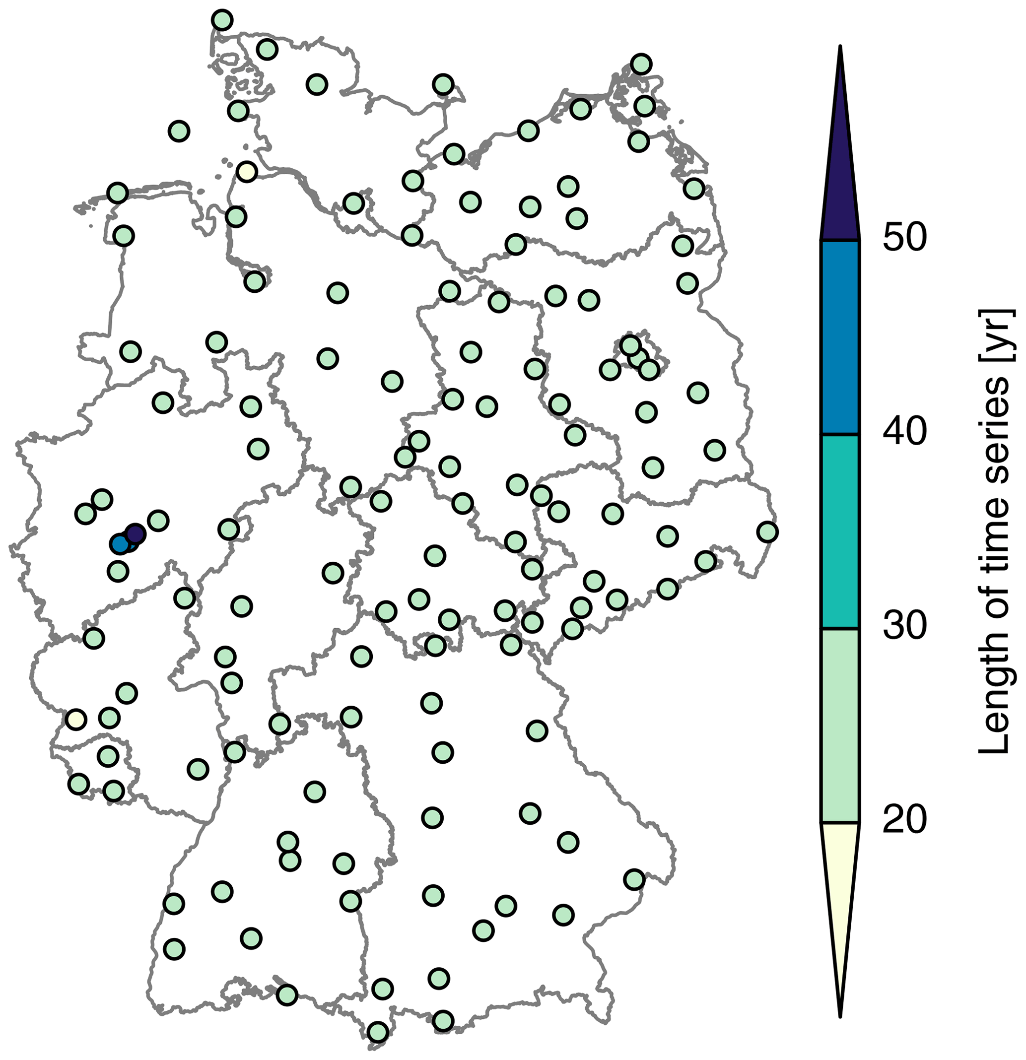
Figure 1Map of Germany with positions of all 132 stations considered. Colors represent the length of the available time series with minute resolution. The longest observation period of 51 years exists for station Bever-Talsperre (dark blue).
The observations were accumulated to the following durations: , with the longest duration 8192 min ≈ 5.7 d, thus resulting in 14 time series per station. Of each time series, we consider both the monthly and annual maxima. Blocks are excluded from the analysis if they contain more than 10 % missing values.
2.2 Modeling annual maxima of different durations
The challenge in modeling extremes is to estimate probabilities of very rare events or those not even observed yet. Here, we apply the block maxima approach which is commonly used for this purpose. It is based on the Fisher–Tippett–Gnedenko theorem, which essentially states that under certain assumptions the probability distribution of block maxima can be modeled by the generalized extreme value (GEV) distribution (Coles, 2001).
More precisely, let X1, … Xn be a sequence of n random variables which are independent and identically distributed (iid), with an unknown distribution. We denote the maximum of this sequence as
In the limit of large block sizes n, the non-exceedance probability can be approximated by the generalized extreme value (GEV) distribution
if for n→∞ the distribution of properly rescaled Mn converges to a nondegenerate distribution. The GEV distribution
is defined on and has three parameters: location parameter , scale parameter σ>0, and a shape parameter . Thus, the position and width of the distribution are specified by μ and σ, respectively, whereas ξ determines the right tail behavior, resulting in bounded right tails for ξ<0 and polynomial decay for ξ>0. In the case ξ=0, Eq. (3) is interpreted in the limit of ξ→0, leading to the Gumbel distribution, with an exponentially decaying tail.
The GEV distribution is thus likely to be a well suited model for the distribution of annual precipitation intensity maxima of one selected aggregation duration. In order to model the distribution for different durations simultaneously, Koutsoyiannis et al. (1998) proposed that the empirical relationship between precipitation intensity and duration can be directly used to model the parameters of the GEV distribution depending on duration, which leads to a duration-dependent GEV (d-GEV) distribution . The relationship between precipitation intensity I and duration d for a chosen non-exceedance probability p corresponds to the quantile qp(d) of the d-GEV distribution:
hence IDF curves can be estimated in a consistent way (Ulrich et al., 2020). For the empirical dependence of the parameters on duration, we follow the assumptions of Koutsoyiannis et al. (1998):
with re-parameterized location parameter , scale offset σ0>0, duration offset θ≥0, and duration exponent . These assumptions are commonly used (Lehmann et al., 2013; Van de Vyver, 2015; Stephenson et al., 2016; Ritschel et al., 2017), however, it may be beneficial to introduce additional parameters (Van de Vyver, 2018; Fauer et al., 2021). By inserting assumptions (Eqs. 5–7) into Eq. (3), we obtain the d-GEV distribution with five parameters
which constitutes a model for the distribution of annual precipitation maxima for a range of durations.
2.3 Modeling monthly maxima
According to the Fisher–Tippett–Gnedenko theorem, the GEV distribution is an adequate model for block maxima if the block size is sufficiently large. For geophysical applications, such as modeling extreme precipitation, it is common to choose a block size of 1 year, as explicit modeling of seasonality is thereby avoided. However, this results in two major disadvantages: large portions of the data are lost for the analysis if only the annual maxima are used, and the assumption that precipitation events originate from an identical distribution is violated if a distinct intra-annual cycle exists. Therefore, the use of a smaller block size is worth considering. Multiple studies suggest that the GEV distribution is well suited to model monthly block maxima of daily precipitation sums in the midlatitudes (Maraun et al., 2009; Rust et al., 2009; Fischer et al., 2018). Similarly, we use monthly maxima to model extreme precipitation of different durations: either with separate models for each duration using the GEV (Eq. 3) or simultaneously using the d-GEV distribution (Eq. 8). Inspection of the quantile–quantile (q–q) plots indicates that the d-GEV distribution is a reasonable approximation for the distribution of monthly maxima at the regarded stations. The q–q plots for station Bever-Talsperre with respect to each month are shown in Fig. S1 in the Supplement.
To account for any form of variability in the GEV model (Eq. 3), the GEV parameters can be modeled as linear functions of covariates xi within the framework of vector generalized linear models (VGLMs) (Yee and Stephenson, 2007):
where φ0 represents the intercept, and are the regression coefficients. The choice of the parameter specific link function lφ(⋅) can ensure that parameters stay within a predefined range. However, we employ the identity lφ(φ)=φ as link function for all parameters. Following Fischer et al. (2018), the intra-annual variations of the GEV parameters can be modeled as a periodic functions of the day of the year (doy) using a series of harmonic functions with a fundamental period of 1 year:
where J is the maximum order of harmonic functions. To obtain the parameters for each month, Eq. (10) is evaluated at the corresponding center days of each month. We model the seasonal variations of the d-GEV distribution in exactly the same way. Essentially, this means that each of the parameters can be expressed in the form of Eq. (10).
2.4 Parameter estimation
The parameters of the GEV distribution can be estimated from a time series of observed block maxima. For this purpose, we apply the widely used maximum likelihood estimator (MLE) (Coles, 2001). Thus, the parameters are chosen by optimizing the likelihood
where the parameter vector contains the unknown GEV parameters, the vector Z consists of the observed maxima zn for different blocks (years/months) n, and g(zn;ϕ) is the probability density function of the GEV distribution. This can be applied analogously for the d-GEV distribution:
Whereas in this case the parameter vector , Z now contains all observed maxima zn for different blocks (years/months) n and durations d, and is the probability density function of the d-GEV distribution. A benefit of the MLE is that it can be easily extended in the case of using covariates to model the parameters (Eq. (10)). The parameter vector then contains the parameter intercepts φ0 and regression coefficients and for each parameter in the case of both GEV and d-GEV distribution.
Since the logarithm of the likelihood reaches the maximum at the same value but is easier to calculate, the parameters are estimated by optimizing the log-likelihood numerically:
It is possible to derive the uncertainty of the parameter estimates, i.e., the variance–covariance matrix, via the Fisher information matrix estimated in this process.
Nevertheless, Eqs. (11) and (12) are only valid if the block maxima are independent of each other. The assumption that maxima of different years or also months are independent is reasonable. However, a dependency exists between the maxima of different durations. Jurado et al. (2020) have shown that accounting for asymptotic dependence between durations yields a modest improvement in the estimation of quantiles of short durations d≤10 h but comes at the cost of increased model complexity. We therefore decide to neglect the dependence between durations when estimating the d-GEV parameters using Eq. (12). Yet, the dependence between durations is taken into account when estimating the uncertainties of the quantiles using the bootstrap method (see Sect. 2.6).
2.5 Model selection
To obtain a parsimonious model, we use a selection procedure consisting of two steps: in the first step, we determine for which of the GEV/d-GEV parameters the modeling of the intra-annual variations is not appropriate and which should therefore remain constant. In the second step, we select which terms of the harmonic series in Eq. (10) are actually needed in order to model the nonconstant parameters.
When modeling intra-annual variations of GEV parameters, the shape parameter ξ is often assumed to be constant (Maraun et al., 2009; Rust et al., 2009; Fischer et al., 2018). This is justified by the fact that ξ controls the tail of the distribution, and thus the estimation of ξ is already associated with large uncertainties. Hence, adding additional coefficients to the estimation of ξ is only reasonable if there are sufficient data available. Fischer et al. (2019) demonstrated that modeling the intra-annual variations of ξ can indeed improve the GEV model. However, their model is able to combine the observations of many stations – due to additional spatial covariates – and therefore the amount of data on which the estimation is based is increased. Since in contrast we employ separate models for each station, we choose the shape parameter to remain constant ξ(doy)=ξ0. For the parameters μ(doy) and σ(doy), a variation in the form of Eq. (10) is adopted.
To be consistent, we also use a constant shape parameter in the d-GEV case. The estimation of the duration offset parameter θ is likewise associated with considerable uncertainties because it is strongly influenced by the estimation of the parameters η and σ0. Equation (5) clearly indicates this effect. Therefore, we choose for θ to remain constant θ(doy)=θ0 as well. The parameters , and η(doy) are allowed to vary periodically throughout the year according to Eq. (10).
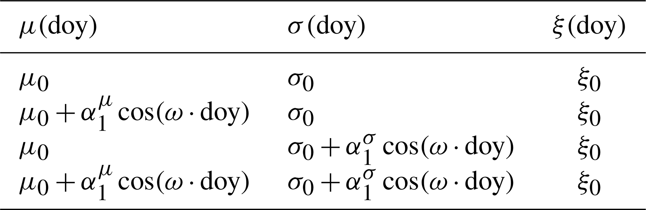
For the maximum order of the harmonic series in Eq. (10), we choose J=4. This results in a maximum of eight regression coefficients and for each nonconstant parameter. Thus, in the GEV case, one would obtain one model per duration containing parameters and in the d-GEV case one model describing all durations simultaneously with parameters to be estimated. To reduce this number to a level where the model describes the variations sufficiently well without overfitting, we apply a stepwise forward regression. For both the GEV model and the d-GEV model, we use the same methods to select the necessary predictor terms: as a model selection criterion, we use the cross-validated log-likelihood. For this purpose, the observations are divided into a training set and a test set, and ln [ℒ(ϕ∣Z)] is computed as in Eqs. (11) and (12), where the parameter vector ϕ is estimated based on the training set, and the observations Z originate from the test set. We choose a small number of folds k=2, as recommended for cross-validation with the aim of model selection (Arlot and Celisse, 2010). Thus, the data are divided into two sets, each of which is used once as a training and once as a test set. In the first step of the stepwise regression, we compare all possible models that can result from the addition of the cosine term with j=1 as covariate for the nonconstant parameters. This yields four possible models for the GEV case, listed in Table 1, and analogously eight models for the d-GEV case. The model resulting in the maximum cross-validated likelihood is retained for the next model selection step. In this next step we similarly identify the nonconstant parameters for which the addition of the sine term with j=1 results in an improvement of the model. We proceed to the maximum order J=4 accordingly.
Table 1All possible models in the first step of the stepwise regression (GEV case) with .
For the station Bever-Talsperre, the resulting estimated d-GEV parameters are presented in Fig. 2. For comparison, the estimated parameters resulting from using a separate model for each month are shown as well. In the case of the station Bever-Talsperre, model selection yields a model with 16 parameters to be estimated. This represents a large parameter reduction compared to using one separate d-GEV model per month with parameters. From Fig. 2, we can note that the choice to keep the parameters ξ and θ constant seems to be justified. In addition, the parameters σ0 and η show a clear variation throughout the year. The estimates of the separate models per month and the d-GEV model with covariates agree well for these two parameters. In the case of the modified location parameter , the variations are not as pronounced as for σ0 and η, so it might be possible to model this parameter as constant as well. However, following Eq. (6), setting would enforce the annual cycle of the location parameter μ(d) and the scale parameter σ(d) to be in phase for any fixed duration d. Based on the results of an exploratory analysis (see Sect. S3), we conclude that the assumption of phase equality of μ(d) and σ(d) for each duration may be too restrictive. Therefore, we decide to allow variations in throughout the year.
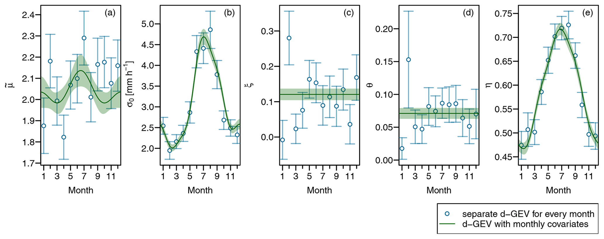
Figure 2Estimated d-GEV parameters , σ0, ξ, θ, and η (a–e) for station Bever-Talsperre: through applying one separate d-GEV model for each month (blue dots) and by modeling all month simultaneously using a d-GEV model with monthly covariates (green lines). The error bars and shaded areas show the 95% confidence intervals obtained via the estimated Fisher information matrix.
2.6 Obtaining IDF curves
When modeling the annual maxima with the d-GEV distribution according to Eq. (8), we can derive IDF curves that correspond to the annual exceedance probabilities using Eq. (4). Likewise, when modeling monthly maxima using the d-GEV distribution with monthly covariates (Eq. 10), Eq. (4) yields separate IDF curves for each month of the year. These correspond to the probabilities that a certain intensity will not be exceeded within a specific month. To distinguish between these two types of IDF curves, we refer to them as annual and monthly IDF curves, respectively.
However, we can also derive annual IDF curves, i.e., quantiles of the distribution of annual maxima, from modeling the monthly maxima. Assuming the maxima of all months in a year as independent, the non-exceedance probability p of an intensity level qp,d within 1 year is derived from its monthly non-exceedance probabilities as
for a fixed duration d. Therefore, to obtain the quantiles of the distribution of annual maxima, we numerically solve Eq. (14) for qp,d, where qp,d is the quantile corresponding to the exceedance probability 1−p, sometimes interpreted as the return level associated with the return period . We compute qp,d for the entire duration range to yield the annual IDF curves.
We determine the uncertainties of the estimated IDF curves using the ordinary nonparametric bootstrap percentile method (Davison and Hinkley, 1997). In this process, a sample is first created from the data by drawing with replacement. This sample is used to estimate the model parameters, from which a certain intensity quantile dependent on duration Ip(d) is then calculated using Eq. (4). By repeating this process R=500 times, we obtain a distribution of intensity quantiles. Finally, the empirical 0.025 and 0.975 quantiles of the bootstrap distribution are used as the lower and upper bounds of the 95 % confidence interval for Ip(d). We assume that considering an appropriate sampling strategy, this method accounts for the dependence between maxima of different durations. For this purpose, all maxima from a particular year are jointly sampled; thus we obtain a sample of n years matching the length of the station time series. Fauer et al. (2021) demonstrated in a sampling experiment that the coverage of the 95 % confidence intervals obtained in this manner stays adequate, even when the dependence of the maxima of different durations is increased.
To visualize the differences between the annual IDF curves resulting from the different models, it can be useful to compare the parameters of the respective distributions of annual maxima. Unfortunately, these are only directly available when modeling the annual maxima. However, we can assume that the distribution of the annual maxima resulting from modeling the monthly maxima is for each duration again a GEV distribution, due to its max-stability property. Thus, we estimate the GEV parameters of the distribution of annual maxima by firstly using Eq. (14) to estimate the quantiles in the range and through inversion obtaining p(qp,d). We then fit the GEV distribution to p(qp,d) using the nonlinear least-squares method to estimate μd, σd, and ξd:
The uncertainties of the estimates of μd, σd, and ξd are likewise determined using the described bootstrap method.
2.7 Verification
We apply a verification procedure in order to assess the estimated quantiles, i.e., IDF curves. At a given station, we aim to compare the annual IDF curves obtained by modeling the monthly maxima with those obtained by modeling the annual maxima. We model the monthly maxima using the d-GEV distribution with monthly covariates according to Eqs. (8) and (10). We abbreviate this model as monthly d-GEV in the following. For modeling the annual maxima, we use the d-GEV distribution (Eq. 8) and abbreviate this model as annual d-GEV.
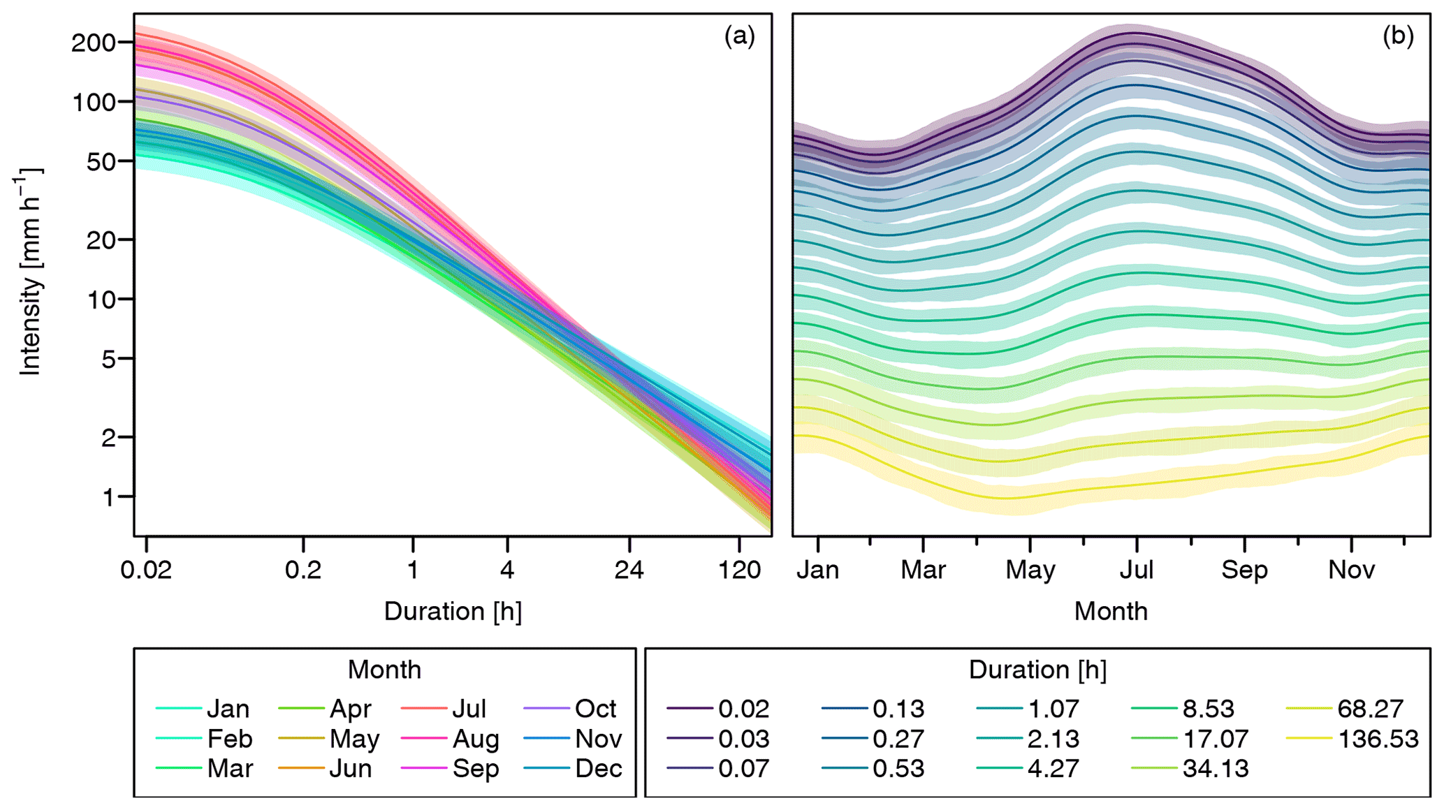
Figure 3The 0.9 quantiles for station Bever-Talsperre for each month (a) and for various durations (b). The durations shown correspond to the durations min discussed in Sect. 2.1. Shaded areas represent the 95 % confidence intervals obtained via the bootstrap method.
To provide a detailed analysis we follow Ulrich et al. (2020), who suggest a verification strategy that allows the estimated quantiles for each duration d and probability p to be examined separately. The approach is based on the comparison of the observations on with the modeled quantile qp via the quantile score (QS) (Bentzien and Friederichs, 2014):
where the check-loss function ρp(u) is evaluated at . To obtain the out-of-sample performance of the model, QS is evaluated in a cross-validation setting (Wilks, 2011). For this purpose, we split the available time series at a station into ny sets, corresponding to the length of the time series in years, by removing the maxima of all durations of a specific year y for each set. The model parameters and thus the quantile qp,d are estimated based on the remaining data. The quantile score for a cross-validation set is calculated from qp,d and the respective omitted observed annual maximum od,y. Therefore, the cross-validated quantile score results in
To compare the score of the monthly d-GEV with that of the annual d-GEV , we use the quantile skill index (QSI) (Ulrich et al., 2020) that is based on the quantile skill score (Wilks, 2011):
Therefore, , where negative values indicate a superior performance of the annual d-GEV model, whereas positive values indicate a superior performance of the monthly d-GEV model.
We first show the results for the monthly IDF curves at the station Bever-Talsperre. Based on the probability that the annual p quantile is exceeded within a certain month, we investigate the seasonal variations of the IDF relationship across Germany. We present the results in detail for six selected stations. Furthermore, we examine the annual IDF curves resulting from modeling monthly maxima and compare them to those obtained from modeling annual maxima. We present the resulting annual IDF curves together with the verification results for three example stations. Since the annual IDF curves derived from the monthly maxima deviate from our original assumptions about the duration dependence, we finally investigate the dependence of the estimated GEV parameters on duration using annual and monthly maxima, respectively. We focus in detail on the shape parameter.
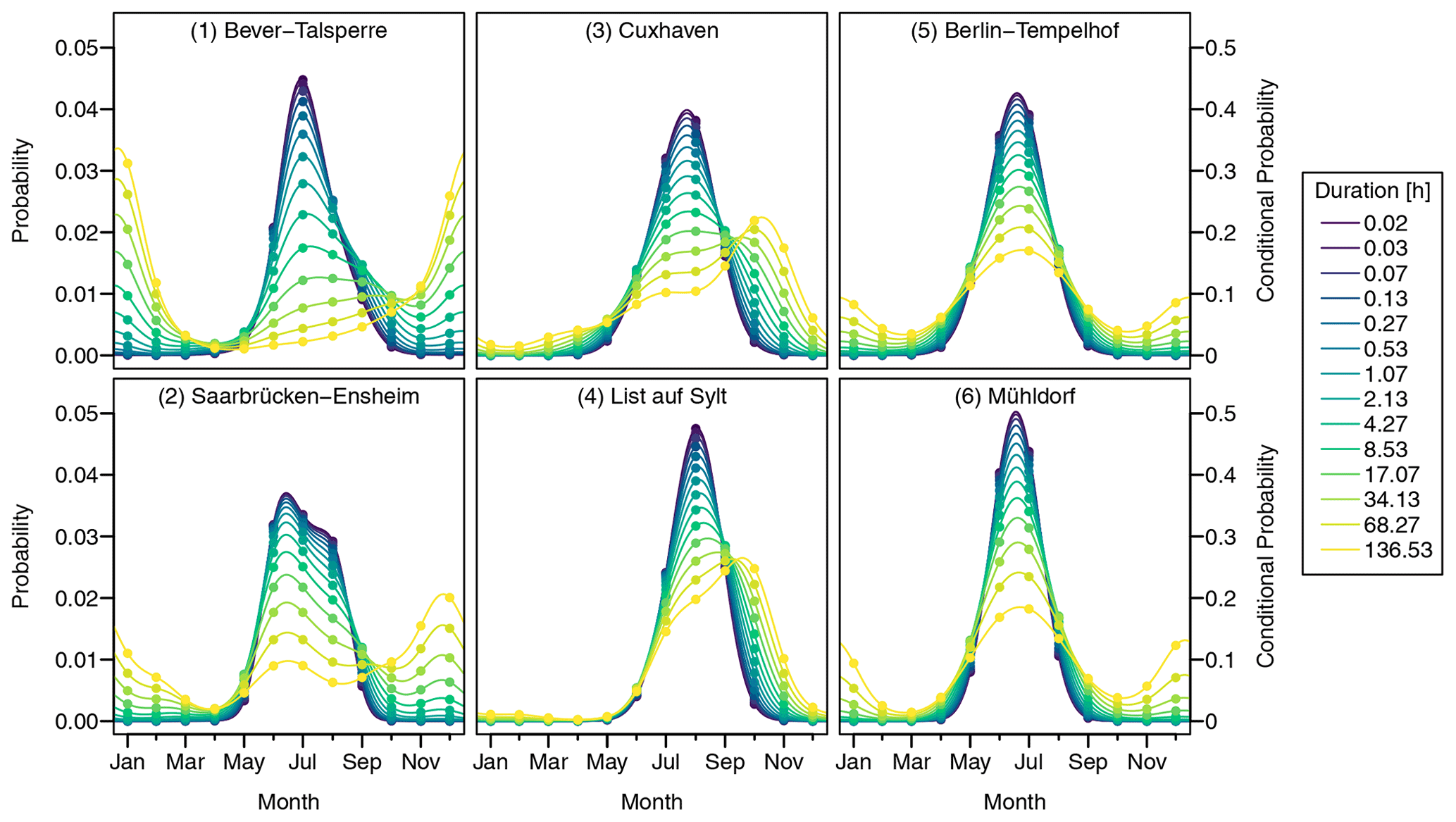
Figure 4Probability of the annual 0.9 quantile q0.9,d being exceeded in a given month. Dots indicate the probability that q0.9,d is exceeded in a certain month, while each point in a line can be interpreted as the probability that q0.9,d is exceeded within the surrounding block of 30 d. To illustrate the interpretation, the product of all probability values presented as dots for a chosen duration results in the annual exceedance probability . Therefore, dividing the probability values by 0.1 yields the conditional probability of exceeding q0.9,d in a given month. For reasons of visual clarity, confidence intervals are not presented. Station names are listed at the top of each plot, while the numbers indicate their positions in Fig. 5.
3.1 Intra-annual variations
We obtain quantile estimates, i.e., IDF curves, for each month using the d-GEV distribution (Eq. 8) with monthly covariates (Eq. 10), through Eq. (4). In the case of the monthly IDF curves, p indicates the probability that the value of the p quantile will not be exceeded within a given month. The 0.9 quantile for each month dependent on duration is shown in Fig. 3a for the station Bever-Talsperre. The IDF curves exhibit a steeper slope in the summer months (pink) than in the autumn and winter months (blue). This is related to the duration exponent η, which exhibits higher values in summer than in winter (Fig. 2e). This result matches the findings of Willems (2000), who determined the rate of exponential decline β of intensity with duration (equivalent to η) for different seasons and likewise found that β exhibits the smallest values in the winter season. For short durations d≤1 h, the intensities reach their maximum in the summer months and their minimum in the winter months. This corresponds to the scale offset parameter σ0, which similarly peaks in summer (Fig. 2b). In contrast, the intensity maximum of long durations d≥24 h occurs in winter and the minimum in spring and summer, since the curves for different months intersect at d≈8 h. The annual variation of the intensity for the different durations is presented in Fig. 3b. It is evident that the intensity maximum shifts from summer for the short durations (purple/ blue) through autumn into winter for the long durations (light green/ yellow). Here, only the quantiles of the monthly distributions for p=0.9 are shown. However, the monthly quantiles for other probability values exhibit the same behavior. The intersection of the IDF curves and the resulting change in seasonality for different durations is not generally present at all stations in the investigated duration range. However, since different duration exponents of the curves in summer and winter occur at all stations, we suspect that at all stations, given sufficiently long durations, the intensity maximum moves into winter eventually.
Due to the exponential decrease of intensity with duration, a comparison of the p quantiles of different durations is only possible on a logarithmic intensity scale. However, the interpretation of a logarithmic axis is often difficult. Therefore, in addition to the monthly 0.9 quantiles presented in Fig. 3, we will also consider the probabilities that the annual 0.9 quantile is exceeded within a given month. To do this, we first use Eq. (14) to calculate the annual quantiles qp,d (return values) from the monthly non-exceedance probabilities. Based on this, we calculate the probability that qp,d will be exceeded within a given month. Figure 4 (upper left) presents the probabilities that the annual 0.9 quantile q0.9,d (10-year return value) for different durations will be exceeded within a given month at the Bever station. This depiction is a useful complement to Fig. 3, since the probabilities for different durations vary on a linear scale, unlike the intensities. The monthly exceedance probability for short durations d<1 h (purple/ blue) exhibits a sharp peak with a maximum in July. The probability that is exceeded in the months November to April is approximately zero. This means that extreme events of short duration, i.e., caused by convective precipitation cells, are likely to occur in summer, while the probability of these events occurring in the months October to April is very small. This is consistent with the results for one station in Belgium (Willems, 2000). In the transition to longer durations, the probability decreases in July, while a second maximum occurs in December to January. For durations of about 8 to 17 h, this results in an extended period of time ranging from June to February, during which the probability shows similarly elevated values. For the long durations d>48 h (light green/yellow), the probability again has one clear maximum, which occurs in December to January. The probability of being exceeded in the months April to June is relatively low in this case. Therefore, these long-lasting extreme events, i.e., frontal events, are more likely to occur in late autumn or winter.
To investigate the intra-annual variations across Germany, we calculate the probability that the annual p quantile is exceeded in a given month for each station. We present the results for p=0.9 in Fig. 5, whereby a different choice of p yields very similar results. We summarize the information on a map by indicating the maximum probability (size of the dots), as well as the month in which the maximum occurs (color of the dots). To a certain extent, the maximum probability provides information about the shape of the curve: a high maximum probability is associated with a narrow probability peak. This implies that the probabilities in the remaining months of the year are comparatively small. In contrast, a small maximum probability suggests that there are other months in the year with similar probability values.
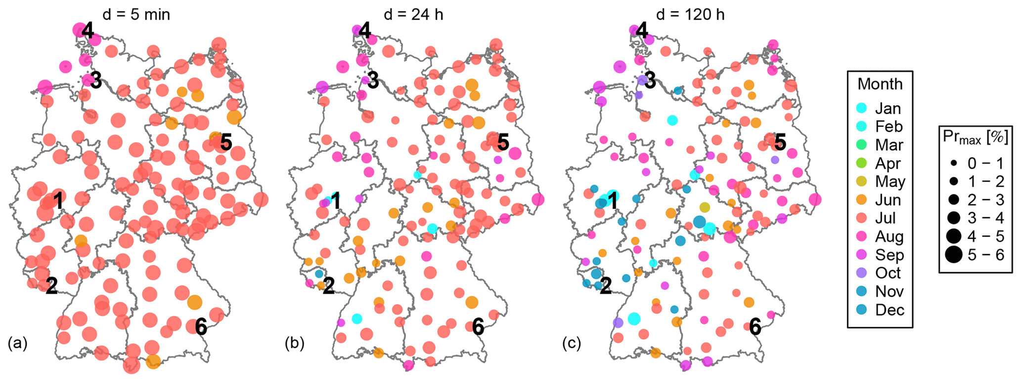
Figure 5Maximum probability of the annual 0.9 quantile qp,d being exceeded in 1 month and months when the maximum occurs at each of the considered stations for three different durations. Dividing the probability values by the annual exceedance probability yields the conditional probability. Therefore a value of Prmax=5 % can be interpreted as 50 % of the exceedances of qp,d occurring in a single month. Numbers indicate the locations of example stations, presented in more detail in Fig. 4.
From Fig. 5a it is evident that for short durations the probability peaks in summer at every station, specifically in July at most stations. There are also some stations where the maximum occurs in June or August. Noticeably, the stations where the maximum is in August are all located on the North Sea coast. Furthermore, at most stations the maximum probability is greater than 3 %, which indicates a narrow probability peak in summer for short durations. When comparing the maximum probabilities with those at d=24 h (Fig. 5b), we find that the maximum probability decreases considerably at almost all stations, thus broadening the time window within which the annual 0.9 quantile is more likely to be exceeded. At most stations, the maximum occurs in the period from June to September. At six stations, however, the maximum is reached in December or January. These stations are all located at higher altitudes (Mittelgebirge). Figure 5c for d=120 h reveals a comparatively heterogeneous spatial distribution, both in terms of the maximum probability and the months in which the maximum occurs. At most stations in Germany, the maximum still lies between June and September; however, the number of stations with maximum probability between November and January is considerably increased in the west of Germany, especially in higher regions.
Regarding the month with the highest probability in the case of long durations, we derive a rough division of the stations within Germany into three types. For each type we choose two stations, for which we present the probabilities in detail in Fig. 4. We separate the stations into those with a maximum in late autumn and winter (1, 2), between September and October (3, 4), and in summer (5, 6). The locations of the stations are indicated by numbers in Fig. 5.
Station (1) is Bever-Talsperre, which has already been discussed in detail. Similarly to (1), the maximum at the station Saarbrücken-Ensheim (2) also shifts from summer for short durations into late autumn to winter for long durations. The stations differ, however, insofar as the maximum probability for short durations at station (2) in July varies only slightly from the probability in the months of June and September. In addition, the probability for long durations remains rather high in summer, in contrast to station (1). Stations that show a similar shift of the maximum exceedance probability, from summer for short durations to late autumn or winter for long durations, are located exclusively in the western half of Germany and also occur mostly at higher altitudes. The exception are two stations in northern Germany. The location of these stations coincides well with the results of Fischer et al. (2018). They explain the increased occurrence of longer-lasting extreme events in these regions in late autumn and winter, with the stronger westerly winds during these months, which cause particularly high precipitation amounts on the windward sides of the mountain chains (Mittelgebirge) due to the forced uplift of the air. However, this study is based on daily precipitation sums. The fact that when modeling several durations simultaneously, the seasonal variations are observed at longer durations than when modeling a single duration might be due to the smoothing of the seasonal signal.
As examples for stations where the maximum occurs in September or October, for long durations, we present the monthly exceedance probabilities for Cuxhaven (3) and List auf Sylt (4). At both stations the width of the probability peak increases for long durations, while its maximum shifts. This shift is more pronounced at station (3). The probabilities in the interval between December and May are relatively low at both stations for all durations. Some stations of this type are located scattered throughout Germany. However, a clear cluster of these stations exists on the North Sea coast. This group is also characterized by extreme convective precipitation events occurring most likely in August, which could be related to the water temperature in this region reaching its maximum during this month. Accordingly, a possible explanation for the high probability of long-lasting heavy precipitation in the following months might be that extratropical cyclones transport air, which was warmed over the North Sea and thus features a high water content, into this region.
Examples of stations where the probability maximum for all durations occurs in summer are Berlin-Tempelhof (5) and Mühldorf (6). An essential difference to the stations (3) and (4) is that in this case a second maximum occurs in winter for long durations. At station (6) this second maximum is even almost as high as the one in summer for d>120 h. Stations of this type occur everywhere in Germany but are the prominent station type in the eastern half of Germany. The example stations (5) and (6) show a very distinct behavior for the probabilities with increasing duration. At most of the other stations of this type, the signal for longer durations is less clear, as sometimes several maxima occur, or the summer maximum might be shifted by 1 or 2 months. However, the common characteristics of these stations continue to be the maximum for all durations occurring in the period between May and October and the probability for long durations showing similarly increased values throughout several months of the year.
The monthly exceedance probability is a useful indicator of the months from which the annual maxima of different durations originate. For all stations, the peak of the probability is relatively narrow for short durations, with the maximum in summer. The probability that the annual 0.9 quantile occurs in one of the other seasons is negligible. This fact contradicts the assumption of the block maxima approach that precipitation intensities are identically distributed within the block of 1 year. In other words, a block size of 1 year for short durations results in a much smaller effective block size of about 4 to 6 months. With respect to longer durations, the stations differ greatly, but it can be generally stated that the effective block size increases for long durations. Thus, the annual maxima at a station for different durations originate from effective blocks of different sizes, which might even be in different seasons, depending on the station's location. This effect is further emphasized in Fig. S2. Modeling the monthly maxima, on the other hand, avoids this problem. Therefore, in the following section we compare the annual IDF curves derived from annual maxima with those derived from monthly maxima.
3.2 Annual IDF curves
We obtain the annual IDF curves and their confidence intervals from modeling annual and monthly maxima, using the respective methods described in Sect. 2.6. We compare the estimated quantiles from both models along with the QSI described in Sect. 2.7. Figure 6 presents the IDF curves (lower panels) together with the QSI (upper panels) for three example stations. In addition to the station Bever-Talsperre (1), with the longest time series, we present the results for the stations Saarbrücken-Ensheim (2) and Cuxhaven (3), since these three stations cover a broad spectrum in terms of differences between the quantile estimates obtained by both models as well as their uncertainties. The QSI is used to compare the performance of both models. Positive values (red) indicate an increase in the skill of the monthly d-GEV model compared to the annual d-GEV model, while negative values (blue) indicate that the annual model is superior. The result of the QSI may be less reliable if the length of the time series T is shorter than the period corresponding to the non-exceedance probability being verified. Therefore, we indicate the length of the time series available for verification by dots in the upper panels in Fig. 6.
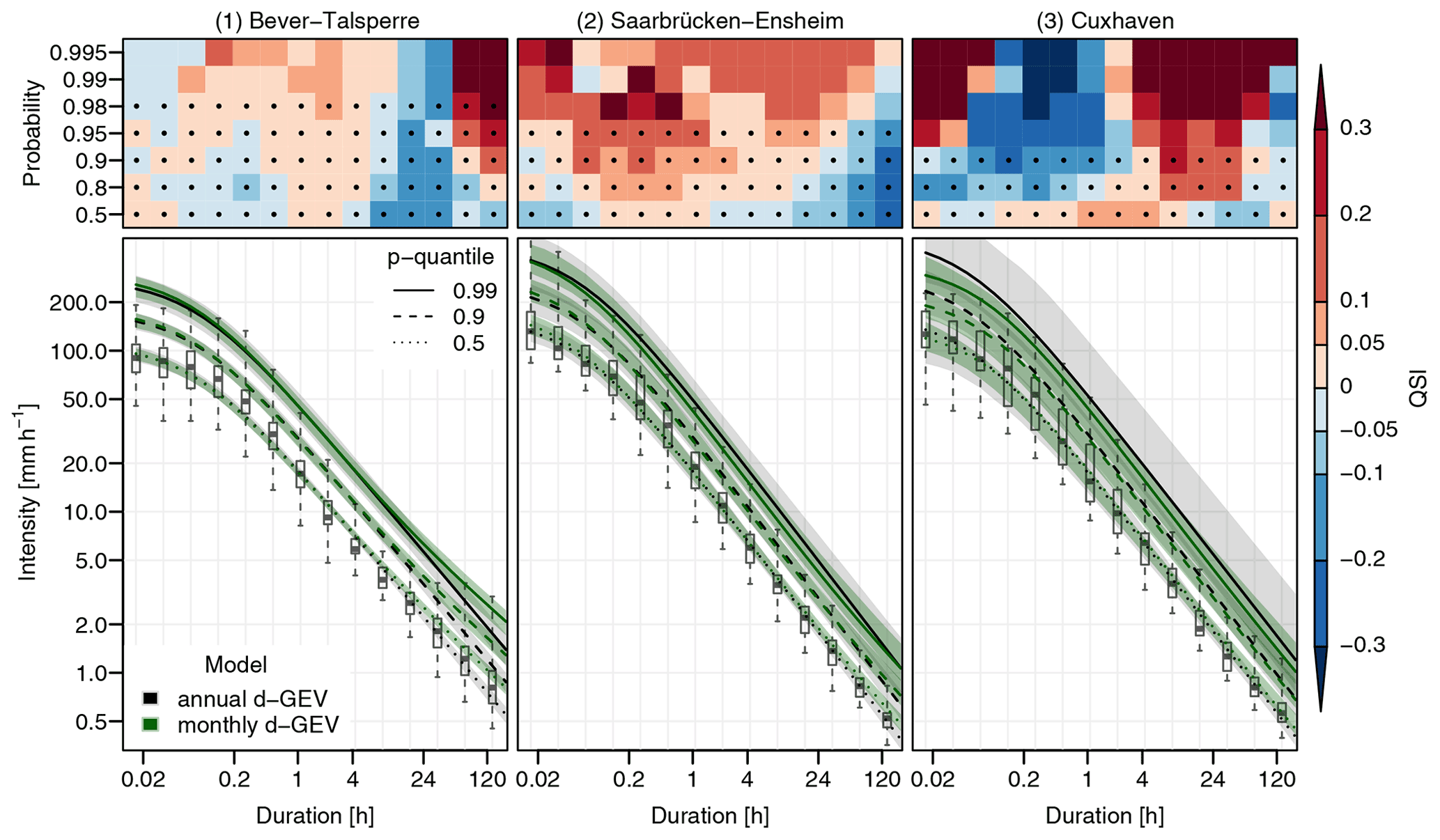
Figure 6Annual IDF curves for three example stations estimated via two models: modeling annual maxima with the d-GEV distribution and modeling monthly maxima using the d-GEV distribution with monthly covariates. The shaded areas represent the respective 95 % confidence intervals. The distributions of the observed annual maxima are shown as box-and-whisker plots, where the whiskers cover the complete data range. In the upper panels the corresponding QSI values are presented, indicating the comparison of the models' performances, where positive values indicate an increase in the skill of the monthly d-GEV model compared to the annual d-GEV model.
For the station Bever-Talsperre, the IDF curves resulting from the two different models are almost identical over a long duration range d<8 h. Therefore, in this duration range, the models' performances differ only marginally, indicated by for almost all probabilities. For high probabilities p≥0.98, the QSI suggests a slightly better performance of the monthly model for durations 4 min≤d≲2 h. At d≈8 h the IDF curves of the monthly model start to deviate from those of the annual model. More precisely, the IDF curves of the monthly model no longer exhibit a power-law behavior for d>8 h but decrease more gradually. Due to the larger differences in the IDF curves, the models' performances vary considerably () in this range. However, the sign of the QSI differs for d≲34 h and d≳68 h: for d≲34 h, the data are better represented by the annual model, as indicated by the negative values of the QSI in this range. For d≳68 h and p≥0.95, however, the monthly model is a considerable improvement over the annual model. This is evident both from the strongly positive QSI values in this range as well as directly from the data, shown as box-and-whisker plots, as the maximum of the observations extends above the modeled 0.99 quantile. The models do not differ much with respect to the width of the 95 % confidence intervals.
At station Saarbrücken-Ensheim, the differences in the IDF curves of the two models are more pronounced throughout the entire duration range: the estimated quantiles of the monthly model are higher for very small and very large durations but lower in the range 8 min≲d≲48 h than those of the annual model. Thus, again the monthly model does not comply with a power law. The QSI indicates that the monthly model is mostly an improvement, except for smaller probabilities at longer durations. Since this station provides a shorter time series than station Bever-Talsperre, i.e., only 24 years, the 95 % confidence intervals of the annual model are wider, especially for short durations and high probabilities. This indicates that the monthly model benefits from utilizing more data regarding the uncertainties.
This appears even more prominent at the Cuxhaven station. Since the high-resolution time series at this station covers only 19 years, the uncertainties of the annual model are considerably wider than those of the monthly model. The estimates of the monthly model for the 0.9 quantile and the 0.99 quantile are below the respective estimates of the annual model. The estimates for the 0.5 quantile differ only slightly. The quantiles of the monthly model roughly parallel those of the annual model for longer durations. Thus, the monthly model does not deviate essentially from a power law at this station. The QSI does not provide a clear indication regarding which model better represents the data but fluctuates between positive and negative values. This seems to be in agreement with the observations. The spread of the boxes and whiskers first increases and then decreases over duration. As a result, in the duration ranges with narrower box-and-whisker plots, the monthly model better represents the data, especially for higher quantiles, while the annual model is more suitable particularly for 8 min≤d≲1 h, where the boxes and whiskers are rather broad.
Overall, we find that the differences between the annual and the monthly model are very heterogeneous for individual stations. However, two general statements can be made:
-
Modeling monthly maxima provides a clear improvement in terms of the quantile estimates' uncertainties, especially for stations with short observational time series.
-
Although a power-law behavior for long durations is assumed for the monthly IDF relations, the resulting annual IDF curves can deviate from this behavior and are therefore more flexible.
This deviation from a simple power-law behavior for long durations is consistent with the findings of Willems (2000), who observes a decrease in the rate of exponential decline of intensity with increasing duration. We observe this decrease to be particularly pronounced at the station Bever-Talsperre, where we also find a clear shift of the seasons in which extreme events of different durations occur. We therefore suspect that the lower slope of the annual IDF curves at long durations is related to this shift. Since we aim to better understand this deviation from the original assumptions in Eqs. (5)–(7), in the following section we examine the relationships between the GEV parameters and duration that follow from modeling monthly maxima.
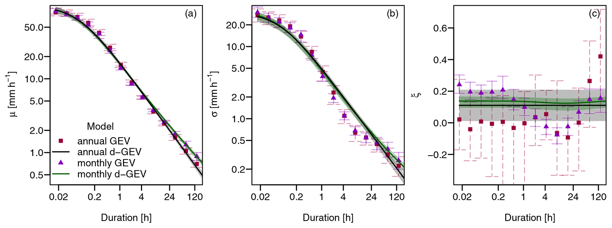
Figure 7Annual GEV parameters μ, σ, and ξ for station Bever-Talsperre estimated via four different models along with bootstrapped 95 % confidence intervals shown as error bars and shaded areas.
In terms of model performance, we likewise cannot draw general conclusions. At some stations, such as Cuxhaven, we find that modeling monthly maxima improves the estimates of the annual IDF curves for almost all probabilities and durations. However, at many stations the improvement in the estimation is limited to a selected range of probabilities and durations, and there are also stations at which the estimated quantiles of the monthly model are always worse than those of the annual model. Since the objective of this study is to model the seasonal variations at all stations by applying a uniform framework, the model selection was performed identically for all stations, e.g., choosing and This results in a varying quality of representation of the parameters at different stations. We expect that parameter estimation for rare events should generally improve, as the introduction of smooth variation during the year allows for the inclusion of additional information. Therefore we assume that with more focus on estimating the IDF curves of a single station, and thus a more targeted choice of model selection approach and initial conditions, the model performance of the monthly model at this station can be considerably improved.
3.3 Duration dependence
To model the IDF relationship, we have so far assumed that the GEV parameters depend on duration according to Eqs. (5)–(7). This results in a power-law behavior, or so-called simple scaling, of intensity with duration except for short durations d<1 h. The curvature of the IDF curves for short durations (in a double-logarithmic plot) is controlled by the parameter θ. Figure 3a illustrates that the IDF curves for each month follow this imposed pattern. However, the resulting annual IDF curves, shown in Fig. 6 in green, deviate from this behavior and thus from the assumptions in Eqs. (5)–(7). To investigate this deviation in more detail, we estimate the annual GEV parameters resulting from modeling monthly maxima, using nonlinear regression according to Eq. (15), separately for each duration. We use the obtained parameters only to compare them with those estimated directly from modeling the annual maxima. They are not intended as a basis of any further analysis. We compare the following four models:
-
modeling annual maxima using
-
a separate GEV distribution for each duration (annual GEV)
-
one d-GEV distribution (annual d-GEV)
-
-
modeling monthly maxima using
-
a separate GEV distribution with monthly covariates for each duration (monthly GEV)
-
one d-GEV distribution with monthly covariates (monthly d-GEV).
-
The annual GEV parameters μ, σ, and ξ estimated via these models are presented depending on duration for the station Bever-Talsperre in Fig. 7 including their respective 95 % confidence intervals. Although the uncertainties of the parameters estimated directly from the annual maxima can be derived using the Fisher information matrix, for comparability, the uncertainties of the parameter estimates are obtained using the bootstrap method described in Sect. 2.6 for all models.
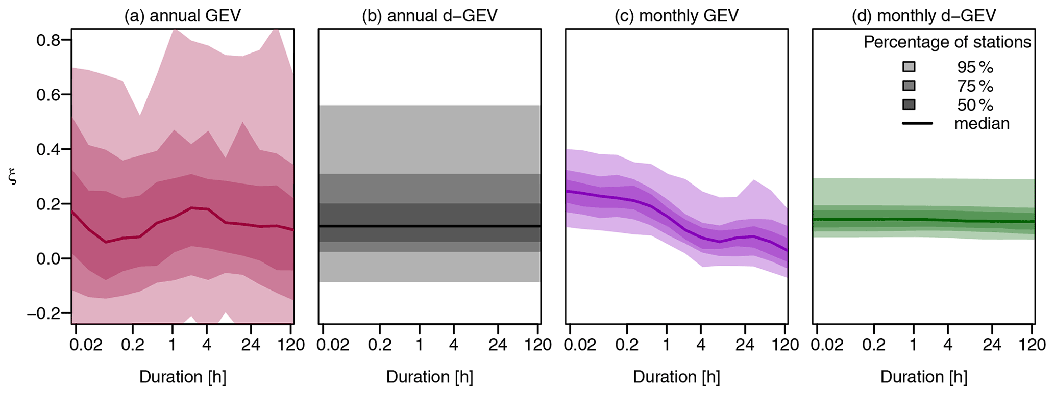
Figure 8Distribution of shape parameter ξ estimated using four different models (columns) at all 132 stations. The shaded areas present the percentage of stations for which the estimated value lies within the respective range, while the line depicts the median value.
For the location parameter μ (Fig. 7a), the estimates of both annual models (red squares and black line) agree well; i.e., μ follows a power law for durations d≥1 h, while the curve decreases more gradually for shorter durations. The estimates of the monthly models (purple triangles and green line) are consistent with those of the annual models for durations d≲24 h; however, both monthly models agree on a slower decline of μ for longer durations d≳24 h and thus a deviation from simple scaling. We observe quite a similar behavior of the model estimates for the scale parameter σ (Fig. 7b): the estimates of all models agree relatively well for short durations d≲1 h, and both monthly models show an upwards deviation from simple scaling for longer durations d≳24 h. However, the estimates of both GEV models (squares and triangles) deviate noticeably from simple scaling towards smaller values in the range 1 h≲d≲24 h. Regarding the uncertainties for the estimates of μ and σ, the annual GEV model (red) is associated with the largest uncertainties. By considering more data, the parameters can be estimated more accurately using the monthly GEV model (purple). Similarly, the annual d-GEV model (black) exhibits considerably smaller uncertainties than the annual GEV model because here the addition of data from other aggregation levels leads to a more confident estimate. Consequently, the joint use of data from all months and durations in the monthly d-GEV model results in the smallest uncertainties regarding parameter estimation. The estimates for μ and σ obtained from all four models agree relatively well at most of the other stations (not presented). Similar to the station Bever-Talsperre, at several stations the estimates of the monthly models show an upward deviation from simple scaling for long durations. The estimates are associated with considerably larger uncertainties for most other stations, where shorter time series are available.
The shape parameter ξ determines the tail of the distribution, and its estimation is therefore subject to relatively large uncertainties depending on the length of the time series. This is similarly the case for the station Bever-Talsperre (Fig. 7c) with a time series of 51 years, where the estimates of ξ based on annual maxima of a single duration (red squares) vary in the range 0.09 to 0.4, but since the 95 % confidence intervals are very broad, it is challenging to derive a relationship between ξ and duration. For the d-GEV we therefore assume a constant shape parameter (Eq. 7), which for the annual d-GEV model (black line) is estimated to be 0.11. Compared to the separate estimates of the annual GEV for each duration (red squares), this value appears reasonable. Additionally, the uncertainties decrease significantly when modeling the annual maxima of all durations simultaneously. For the monthly d-GEV, ξ is also assumed to remain constant over duration for each month. In addition, we hypothesize that ξ does not change throughout the year either, as described in Sect. 2.5. Interestingly, ξ(d) resulting from the monthly d-GEV model (green line) nevertheless deviates slightly from being constant. The estimated values are slightly higher than those of the annual d-GEV model and vary between 0.12 and 0.14, with the minimum at about d≈17 h. Similarly to μ and σ, the uncertainties of the monthly d-GEV model (green) for the estimation of ξ are even smaller than those of the annual d-GEV model (black). When we model the monthly maxima for each duration separately, we benefit from being able to estimate the shape parameter with smaller uncertainties without constraining the relation between ξ and duration. Thus, we observe a distinct variation of ξ estimated via the monthly GEV model (purple triangles) over duration. The estimated values exhibit a minimum, similar to those of the monthly d-GEV model (green line), at d≈8 h and vary in the range −0.08 to 0.24. To evaluate this result, we can visually examine the distribution of annual maxima for different durations, seen in Figs. S2 and 6 (bottom left) as box-and-whisker plots. It is noticeable that the observations for d≈8 h actually cover the smallest range, thus agreeing with the results for the shape parameter.
Since the shape parameter estimates of the four different models vary substantially at the individual stations, we summarize the information for all stations in Fig. 8. For each model, the distribution of the estimated value over all stations is plotted with respect to duration. We observe that ξ estimated using the annual GEV model (red) varies widely among stations. The model seems to only provide estimates in a reasonable range at 75 % of the stations based on the small amount of data. The median of all stations appears to oscillate around a constant value. For the annual GEV model (black), the range in which the estimates vary among stations is narrower, but implausibly high values still occur at some stations. The median is consistent with the median of the annual GEV model (red). In comparison, the range in which the estimated values of the monthly d-GEV model (green) vary is much smaller, and the values are within a reasonable range at all stations. Although in this model ξ is assumed to be constant over duration and months, we see a subtle decrease in the median with duration. Likewise, the variation for ξ between individual stations is smaller for the monthly GEV model (purple) than for either of the annual models (red and black). Additionally, we can see a clear decrease of the shape parameter with duration for this model, since in this case no relation between ξ and duration is predefined.
To summarize, we find that modeling the monthly maxima allows new conclusions to be drawn about the behavior of the parameters of the distribution of annual maxima depending on duration. Instead of using the more complex modeling of monthly maxima to estimate annual IDF curves, one might also try to implement the resulting characteristics directly into the model for annual maxima. We find that for some stations the location μ and scale σ parameters deviate from the assumption of simple scaling toward higher values for long durations. Fauer et al. (2021) showed that this behavior of the parameters can be modeled by an additional parameter τ, called intensity offset. They report that the addition of this parameter for the stations of the Wupper catchment, in which the example station Bever-Talsperre is located, leads on average to an improved estimation of the annual IDF curves for medium to long durations. Regarding the shape parameter ξ, we observe that the reduced uncertainties in the estimation of ξ, resulting from modeling monthly maxima, allow for further investigation of the dependence of ξ on duration. We find that ξ decreases with duration when taking the average of the investigated stations in Germany, reaching values around zero for most stations at long durations. We believe that this finding provides a good basis to explore a potentially more suitable formulation of ξ(d) in future studies. We could imagine that the explicit modeling of this decrease of ξ yields similar results to assuming a different duration exponent for the parameters μ and σ of the d-GEV, so called multiscaling (Gupta and Waymire, 1990; Van de Vyver, 2018). Possibly the latter implementation could be beneficial, since the estimation of these parameters is associated with less uncertainty than that of ξ.
This study focuses on modeling the intra-annual variations of extreme precipitation on different timescales. For this purpose, we employ a duration-dependent generalized extreme value (d-GEV) distribution with monthly covariates. Using this approach allows for the following:
-
investigation of seasonal variations in the intensity–duration–frequency (IDF) relationship;
-
the obtaining of more reliable estimates for the annual IDF curves by utilizing information on extreme events more efficiently;
-
a better understanding of the underlying processes, i.e., the dependence of the parameters on the duration.
Regarding the seasonal variations, we find that everywhere in Germany, the short convective extreme events are most likely to occur in the summer months, whereas there are regional differences for the seasonality of long-lasting stratiform extreme events. Our findings will allow future studies to identify meaningful factors accounting for these regional differences.
Furthermore, our results show that the annual IDF curves based on the monthly maxima constitute a major improvement in terms of uncertainties of the estimates. Using the quantile skill index (QSI), we compare the performance of the models based on the annual and monthly maxima and show that, for some stations, modeling the monthly maxima also leads to a considerable improvement in this regard. A limitation of this study is the strict assumptions that are imposed on the seasonal variations of the distribution parameters. Subsequent studies should therefore investigate the degree to which relaxing these assumptions might further improve the performance of the model based on monthly data. For example, in the framework of a vector generalized additive model (Yee and Stephenson, 2007), it would be possible to model these smooth variations in a nonparametric form. Based on our results, it might be beneficial to model the monthly maxima for obtaining annual IDF curves when there are large differences in the seasonality of extreme events on different timescales, such as at the station Bever-Talsperre, or for stations where only short observation time series are available. However, it must be considered that a misspecification of the seasonal variations of the parameters can lead to poor results. Moreover, modeling monthly precipitation maxima with the GEV may not be possible in regions with very small precipitation amounts during some months of the year. Therefore, the applicability of the model to the data should always be verified.
Finally, we can demonstrate that at some stations the annual IDF curves based on the monthly maxima deviate from the assumption of scale invariance for long durations. We illustrate that this behavior can be captured by a different parameterization of the location and scale parameter. For future research, it might be of interest to compare the monthly model employed in this study with an annual model that uses different parameterization, e.g., the one proposed by Fauer et al. (2021). Moreover, by including additional information in the form of smooth variations during the year, we observe that the shape parameter decreases with duration when averaged over all stations. Based on this result, future research should investigate whether the assumption of a constant shape parameter is appropriate for a wide range of durations from minutes to several days or whether a more appropriate explicit relationship can be identified.
In conclusion, the use of monthly maxima can be beneficial in several respects when estimating IDF curves, even when information on seasonal variations is not required.
The station data are mostly publicly available via the Climate Data Center of the DWD (https://opendata.dwd.de/climate_environment/CDC/observations_germany/climate/1_minute/precipitation/historical/; DWD, 2021). We provide the monthly maxima for 14 aggregation times at all 132 stations, serving as the basis for the analysis, online (https://doi.org/10.5281/zenodo.5025657; Ulrich et al., 2021a). The statistical analysis was performed using the package IDF for the R environment (Ulrich et al., 2020; R Core Team, 2020). The package is available for download at https://CRAN.R-project.org/package=IDF (Ulrich et al., 2021b).
The supplement related to this article is available online at: https://doi.org/10.5194/hess-25-6133-2021-supplement.
HWR and JU conceptualized this study. HWR provided supervision. JU developed the software, carried out the statistical analysis, and evaluated the results. FSF supported the code implementation. HWR and FF contributed to the interpretation of the results. JU prepared the original draft. HWR and FSF revised the draft.
The contact author has declared that neither they nor their co-authors have any competing interests.
Publisher's note: Copernicus Publications remains neutral with regard to jurisdictional claims in published maps and institutional affiliations.
The authors would like to thank the Wupperverband as well as the Climate Data Center of the DWD, for providing and maintaining the precipitation time series. Jana Ulrich kindly appreciates the support and motivation offered by Lisa Berghäuser and Oscar E. Jurado. Finally, we would like to thank Juliette Blanchet and two anonymous referees for their valuable feedback and suggestions to improve the manuscript.
This research has been supported by the Deutsche Forschungsgemeinschaft (grant nos. GRK2043/1, GRK2043/2, and CRC 1114) and the Bundesministerium für Bildung und Forschung (grant no. 01LP1902H).
We acknowledge support from the Open Access Publication Initiative of Freie Universität Berlin.
This paper was edited by Nadav Peleg and reviewed by J. Blanchet and two anonymous referees.
Arlot, S. and Celisse, A.: A survey of cross-validation procedures for model selection, Statist. Surv., 4, 40–79, https://doi.org/10.1214/09-SS054, 2010. a
Barredo, J. I.: Normalised flood losses in Europe: 1970–2006, Nat. Hazards Earth Syst. Sci., 9, 97–104, https://doi.org/10.5194/nhess-9-97-2009, 2009. a
Bentzien, S. and Friederichs, P.: Decomposition and graphical portrayal of the quantile score, Q. J. Roy. Meteorol. Soc., 140, 1924–1934, https://doi.org/10.1002/qj.2284, 2014. a
Berg, P., Moseley, C., and Haerter, J.: Strong increase in convective precipitation in response to higher temperatures, Nat. Geosci., 6, 181–185, https://doi.org/10.1038/ngeo1731, 2013. a
Bronstert, A.: Floods and Climate Change: Interactions and Impacts, Risk Anal., 23, 545–557, https://doi.org/10.1111/1539-6924.00335, 2003. a
Coles, S.: An Introduction to Statistical Modeling of Extreme Values, Springer, London, https://doi.org/10.1198/tech.2002.s73, 2001. a, b, c, d
Courty, L. G., Wilby, R. L., Hillier, J. K., and Slater, L. J.: Intensity-duration-frequency curves at the global scale, Environ. Res. Lett., 14, 084045, https://doi.org/10.1088/1748-9326/ab370a, 2019. a
Davenport, F. V., Burke, M., and Diffenbaugh, N. S.: Contribution of historical precipitation change to US flood damages, P. Natl. Acad. Sci. USA, 118, e2017524118, https://doi.org/10.1073/pnas.2017524118, 2021. a
Davison, A. C. and Gholamrezaee, M. M.: Geostatistics of extremes, P. Roy. Soc. A, 468, 581–608, https://doi.org/10.1098/rspa.2011.0412, 2012. a
Davison, A. C. and Hinkley, D. V.: Bootstrap methods and their application, 1, Cambridge University Press, Cabridge, 1997. a
Durrans, S. R.: Intensity-Duration-Frequency Curves, AGU – American Geophysical Union, 159–169, available at: https://agupubs.onlinelibrary.wiley.com/doi/10.1029/2009GM000919 (last access: 1 December 2021), 2010. a, b
Durrans, S. R., Eiffe, M. A., Thomas, W. O., and Goranflo, H. M.: Joint Seasonal/Annual Flood Frequency Analysis, J. Hydrol. Eng., 8, 181–189, https://doi.org/10.1061/(ASCE)1084-0699(2003)8:4(181), 2003. a
DWD Climate Data Center (CDC): Historical 1-minute station observations of precipitation for Germany, version V1, 2019, https://opendata.dwd.de/climate_environment/CDC/observations_germany/climate/1_minute/precipitation/historical/, last access: 5 March 2021. a
Dyrrdal, A. V., Lenkoski, A., Thorarinsdottir, T. L., and Stordal, F.: Bayesian hierarchical modeling of extreme hourly precipitation in Norway, Environmetrics, 26, 89–106, 2015. a
Fauer, F. S., Ulrich, J., Jurado, O. E., and Rust, H. W.: Flexible and Consistent Quantile Estimation for Intensity-Duration-Frequency Curves, Hydrol. Earth Syst. Sci. Discuss. [preprint], https://doi.org/10.5194/hess-2021-334, in review, 2021. a, b, c, d
Fischer, M., Rust, H. W., and Ulbrich, U.: Seasonal Cycle in German Daily Precipitation Extremes, Meteorol. Z., 27, 3–13, https://doi.org/10.1127/metz/2017/0845, 2018. a, b, c, d, e, f, g
Fischer, M., Rust, H., and Ulbrich, U.: A spatial and seasonal climatology of extreme precipitation return-levels: A case study, Spat. Stat., 34, 100275, https://doi.org/10.1016/j.spasta.2017.11.007, 2019. a, b, c
Friederichs, P.: Statistical downscaling of extreme precipitation events using extreme value theory, Extremes, 13, 109–132, https://doi.org/10.1007/s10687-010-0107-5, 2010. a
Gupta, V. K. and Waymire, E.: Multiscaling properties of spatial rainfall and river flow distributions, J. Geophys. Res.-Atmos., 95, 1999–2009, https://doi.org/10.1029/JD095iD03p01999, 1990. a
Hartmann, D., Klein Tank, A., Rusticucci, M., Alexander, L., Brönnimann, S., Charabi, Y., Dentener, F., Dlugokencky, E., Easterling, D., Kaplan, A., Soden, B., Thorne, P., Wild, M., and Zhai, P.: Observations: Atmosphere and Surface, book section 2, Cambridge Univ. Press, Cambridge, UK and New York, NY, USA, 159–254, https://doi.org/10.1017/CBO9781107415324.008, 2013. a
Hattermann, F. F., Kundzewicz, Z. W., Huang, S., Vetter, T., Gerstengarbe, F.-W., and Werner, P.: Climatological drivers of changes in flood hazard in Germany, Acta Geophys., 61, 463–477, https://doi.org/10.2478/s11600-012-0070-4, 2013. a
Jurado, O. E., Ulrich, J., Scheibel, M., and Rust, H. W.: Evaluating the Performance of a Max-Stable Process for Estimating Intensity-Duration-Frequency Curves, Water, 12, 3314, https://doi.org/10.3390/w12123314, 2020. a
Katz, R. W., Parlange, M. B., and Naveau, P.: Statistics of extremes in hydrology, Adv. Water Resour., 25, 1287–1304, https://doi.org/10.1016/S0309-1708(02)00056-8, 2002. a
Kochanek, K., Strupczewski, W. G., and Bogdanowicz, E.: On seasonal approach to flood frequency modelling. Part II: flood frequency analysis of Polish rivers, Hydrol. Process., 26, 717–730, https://doi.org/10.1002/hyp.8178, 2012. a
Koutsoyiannis, D., Kozonis, D., and Manetas, A.: A mathematical framework for studying rainfall intensity-duration-frequency relationships, J. Hydrol., 206, 118–135, https://doi.org/10.1016/S0022-1694(98)00097-3, 1998. a, b, c
Kunz, M., Mohr, S., and Werner, P. C.: Niederschlag, in: Klimawandel in Deutschland, chap 7, edited by: Brasseur, G., Jacob, D., and Schuck-Zöller, S., Springer Spektrum, Berlin, Heidelberg, 57–66, https://doi.org/10.1007/978-3-662-50397-3_7, 2017. a
Lazoglou, G., Anagnostopoulou, C., Tolika, K., and Kolyva-Machera, F.: A review of statistical methods to analyze extreme precipitation and temperature events in the Mediterranean region, Theor. Appl. Climatol., 136, 99–117, https://doi.org/10.1007/s00704-018-2467-8, 2019. a
Lehmann, E., Phatak, A., Soltyk, S., Chia, J., Lau, R., and Palmer, M.: Bayesian hierarchical modelling of rainfall extremes, edited by: Piantadosi, J., Anderssen, R., and Boland, J., in: Proceedings of the 20th International Congress on Modelling and Simulation (MODSIM), 1–6 December 2013, Modelling & Simulation Society Australia & New Zealand, Adelaide, 2806–2812, 2013. a, b
Linnerooth-Bayer, J. and Amendola, A.: Introduction to Special Issue on Flood Risks in Europe, Risk Anal., 23, 537–543, https://doi.org/10.1111/1539-6924.00334, 2003. a
Łupikasza, E. B.: Seasonal patterns and consistency of extreme precipitation trends in Europe, December 1950 to February 2008, Clim. Res., 72, 217–237, https://doi.org/10.3354/cr01467, 2017. a
Maraun, D., Rust, H. W., and Osborn, T. J.: The annual cycle of heavy precipitation across the United Kingdom: a model based on extreme value statistics, Int. J. Climatol., 29, 1731–1744, https://doi.org/10.1002/joc.1811, 2009. a, b, c, d
Moberg, A. and Jones, P. D.: Trends in indices for extremes in daily temperature and precipitation in central and western Europe, 1901–99, Int. J. Climatol., 25, 1149–1171, https://doi.org/10.1002/joc.1163, 2005. a
Olsson, J., Södling, J., Berg, P., Wern, L., and Eronn, A.: Short-duration rainfall extremes in Sweden: a regional analysis, Hydrol. Res., 50, 945–960, https://doi.org/10.2166/nh.2019.073, 2019. a
Papalexiou, S. M. and Koutsoyiannis, D.: Battle of extreme value distributions: A global survey on extreme daily rainfall, Water Resour. Res., 49, 187–201, https://doi.org/10.1029/2012WR012557, 2013. a
Paprotny, D., Sebastian, A., Morales-Nápoles, O., and Jonkman, S. N.: Trends in flood losses in Europe over the past 150 years, Nat. Commun., 9, 1985, https://doi.org/10.1038/s41467-018-04253-1, 2018. a
R Core Team: R: A Language and Environment for Statistical Computing, R Foundation for Statistical Computing, Vienna, Austria, available at: https://www.R-project.org/ (last access: 15 June 2021), 2020. a
Ritschel, C., Ulbrich, U., Névir, P., and Rust, H. W.: Precipitation extremes on multiple timescales – Bartlett-Lewis rectangular pulse model and intensity-duration-frequency curves, Hydrol. Earth Syst. Sci., 21, 6501–6517, https://doi.org/10.5194/hess-21-6501-2017, 2017. a
Rottler, E., Francke, T., Bürger, G., and Bronstert, A.: Long-term changes in central European river discharge for 1869–2016: impact of changing snow covers, reservoir constructions and an intensified hydrological cycle, Hydrol. Earth Syst. Sc., 24, 1721–1740, https://doi.org/10.5194/hess-24-1721-2020, 2020. a
Rust, H., Maraun, D., and Osborn, T.: Modelling seasonality in extreme precipitation, Eur. Phys. J. Spec. Top., 174, 99–111, https://doi.org/10.1140/epjst/e2009-01093-7, 2009. a, b, c, d
Sebille, Q., Fougères, A.-L., and Mercadier, C.: Modeling extreme rainfall A comparative study of spatial extreme value models, Spat. Stat., 21, 187–208, https://doi.org/10.1016/j.spasta.2017.06.009, 2017. a
Stephenson, A. G., Lehmann, E. A., and Phatak, A.: A max-stable process model for rainfall extremes at different accumulation durations, Weather Clim. Ext., 13, 44–53, https://doi.org/10.1016/j.wace.2016.07.002, 2016. a
Ulrich, J., Jurado, O. E., Peter, M., Scheibel, M., and Rust, H. W.: Estimating IDF Curves Consistently over Durations with Spatial Covariates, Water, 12, 3119, https://doi.org/10.3390/w12113119, 2020. a, b, c, d, e
Ulrich, J., Fauer, F. S., and Rust, H. W.: Monthly precipitation intensity maxima for 14 aggregation times at 132 stations in Germany, Zenodo [data set], https://doi.org/10.5281/zenodo.5025657, 2021a. a
Ulrich, J., Ritschel, C., Mack, L., Jurado, O. E., Fauer, F. S., Detring, C., and Joedicke, S.: IDF: Estimation and Plotting of IDF Curves, r package version 2.1.0 [code], https://CRAN.R-project.org/package=IDF, 2021. a
Van de Vyver, H.: Bayesian estimation of rainfall intensity–duration–frequency relationships, J. Hydrol., 529, 1451–1463, https://doi.org/10.1016/j.jhydrol.2015.08.036, 2015. a
Van de Vyver, H.: A multiscaling-based intensity–duration–frequency model for extreme precipitation, Hydrol. Process., 32, 1635–1647, https://doi.org/10.1002/hyp.11516, 2018. a, b, c
Van de Vyver, H. and Demarée, G. R.: Construction of Intensity–Duration–Frequency (IDF) curves for precipitation at Lubumbashi, Congo, under the hypothesis of inadequate data, Hydrolog. Sci. J., 55, 555–564, https://doi.org/10.1080/02626661003747390, 2010. a
Wilks, D. S.: Statistical methods in the atmospheric sciences, in: vol. 100, Academic Press, Amsterdam, the Netherlands, 2011. a, b
Willems, P.: Compound intensity/duration/frequency-relationships of extreme precipitation for two seasons and two storm types, J. Hydrol., 233, 189–205, https://doi.org/10.1016/S0022-1694(00)00233-X, 2000. a, b, c, d
Yee, T. W. and Stephenson, A. G.: Vector generalized linear and additive extreme value models, Extremes, 10, 1–19, https://doi.org/10.1007/s10687-007-0032-4, 2007. a, b