the Creative Commons Attribution 4.0 License.
the Creative Commons Attribution 4.0 License.
 | 18 Nov 2021
AI-based techniques for multi-step streamflow forecasts: application for multi-objective reservoir operation optimization and performance assessment
Yuxue Guo
Xinting Yu
Haiting Gu
Jingkai Xie
Streamflow forecasts are traditionally effective in mitigating water scarcity and flood defense. This study developed an artificial intelligence (AI)-based management methodology that integrated multi-step streamflow forecasts and multi-objective reservoir operation optimization for water resource allocation. Following the methodology, we aimed to assess forecast quality and forecast-informed reservoir operation performance together due to the influence of inflow forecast uncertainty. Varying combinations of climate and hydrological variables were input into three AI-based models, namely a long short-term memory (LSTM), a gated recurrent unit (GRU), and a least-squares support vector machine (LSSVM), to forecast short-term streamflow. Based on three deterministic forecasts, the stochastic inflow scenarios were further developed using Bayesian model averaging (BMA) for quantifying uncertainty. The forecasting scheme was further coupled with a multi-reservoir optimization model, and the multi-objective programming was solved using the parameterized multi-objective robust decision-making (MORDM) approach. The AI-based management framework was applied and demonstrated over a multi-reservoir system (25 reservoirs) in the Zhoushan Islands, China. Three main conclusions were drawn from this study: (1) GRU and LSTM performed equally well on streamflow forecasts, and GRU might be the preferred method over LSTM, given that it had simpler structures and less modeling time; (2) higher forecast performance could lead to improved reservoir operation, while uncertain forecasts were more valuable than deterministic forecasts, regarding two performance metrics, i.e., water supply reliability and operating costs; (3) the relationship between the forecast horizon and reservoir operation was complex and depended on the operating configurations (forecast quality and uncertainty) and performance measures. This study reinforces the potential of an AI-based stochastic streamflow forecasting scheme to seek robust strategies under uncertainty.
- Article
(11025 KB) - Full-text XML
- BibTeX
- EndNote


Multi-step streamflow forecast is of great importance for reservoir operations to determine optimal water allocations considering the current use and the carry-over storage for mitigating water scarcity risk in the future (Guo et al., 2018; Zhao et al., 2019). Previous studies have identified that real-time reservoir operations are influenced by multiple uncertainties (Xu et al., 2020), among which inflow forecast uncertainty has been determined as the primary source, resulting in the risk of water shortage when the forecast inflow overestimates the actual inflow. Ensemble forecasting techniques are commonly used to characterize various uncertainties in streamflow forecasts. According to comparative analysis for various probabilistic forecasting techniques (Nott et al., 2012; Fang et al., 2018a; Zhai and Chen, 2018; Zhou et al., 2020b), Bayesian model averaging (BMA) (Hoeting et al., 1999) has been found to be an effective and most commonly used method to evaluate uncertainty and thus can be used in streamflow forecast.
Any ensemble forecast approach relies upon model diversity that different models produce, with specific emphasis and different aspects of the features they want to model (Zhou et al., 2020a). In the last few decades, many approaches have been developed to forecast streamflow, including physically based and data-driven models (Tikhamarine et al., 2020; Zuo et al., 2020). Although physically based models can help understand underlying physical processes, they usually require a large amount of input information, such as meteorological and geographic data as well as soil and land use characteristics (Guo et al., 2018, 2020a). Different from physically based models, data-driven models based on statistical modeling have attracted significant interest due to their simplicity and satisfactory forecast results with low information requirements (Al-Sudani et al., 2019; Mehdizadeh et al., 2019; Osman et al., 2020). Artificial intelligence (AI)-based approaches, i.e., machine learning (ML) methods, belong to the latter group. Widely used ML approaches include artificial neural networks (ANNs) and least-squares support vector machines (LSSVMs) (Ghumman et al., 2018; Kisi et al., 2019; Meng et al., 2019; Adnan et al., 2020; Ali and Shahbaz, 2020). Such models have been proven to be efficient tools to model qualitative and quantitative hydrological variables and deal with nonlinear features in streamflow. In recent years, the booming development of deep learning technology has brought many new approaches, such as recurrent neural networks (RNNs) (Elman, 1990), one of the most popular neural networks in the deep learning field. RNNs can preserve and remember the short-past and long-past information and thus are preferred for a complex and highly nonlinear timing problem. Long short-term memory (LSTM) (Hochreiter and Schmidhuber, 1997) and gated recurrent unit (GRU) models (Cho et al., 2014) are two different versions of RNNs. LSTM and GRU networks have been successfully applied in many fields (Greff et al., 2017; Zhang et al., 2018; Jung et al., 2020; Shahid et al., 2020; Ayzel and Heistermann, 2021), and they are demonstrated to generate comparable performances, But GRU has a more straightforward structure and a higher operation speed than LSTM. Recently, many applications that assessed them together are also found in the hydrological field (Gao et al., 2020; Muhammad et al., 2019).
While a considerable research effort has been made to evaluate and improve the quality of streamflow forecasts (Gibbs et al., 2018; Nanda et al., 2019; Sharma et al., 2019; Van Osnabrugge et al., 2019; Feng et al., 2020; Pechlivanidis et al., 2020), how forecasts impact decision-making in the real-time reservoir operations has also gradually gained researchers' attention (Goddard et al., 2010; Shamir, 2017; Anghileri et al., 2019; Alexander et al., 2020; Hadi et al., 2020), e.g., do high-quality forecasts mean improved decision? Traditionally, a skillful forecast is vital for the reliability of the forecasts and is essential to promote the use of forecasts in real-world applications by decision makers. In fact, forecast value is expected to increase with forecast quality, but it may also vary based on other factors such as reservoir capacity and operating objectives (Anghileri et al., 2016). Some studies have even disproved the intuitive assumption that higher forecast performance always leads to better operation decisions, for example, in agricultural water management (Chiew et al., 2003) and water resources allocation (Turner et al., 2017). Therefore, when forecasts are used to support reservoir operation, it should be assessed in which conditions they can help make better decisions. Moreover, forecast uncertainty and error generally grow with the increase of the forecast horizon (Maurer and Lettenmaier, 2004; Denaro et al., 2017; Zhao et al., 2019). A decision maker may doubt whether longer forecast lead times provide sufficient information for a decision purpose or not. There is often a mismatch between the information needed for reservoir operations and the skillful lead time of the reservoir inflow forecast (Anghileri et al., 2016). It is crucial to demonstrate the applicability and effectiveness of the forecast horizon in a forecast-based reservoir operation system (Xu et al., 2014). Overall, there is a continuous need for in-depth study to conduct posterior evaluations of forecasts with different forecast lead times and obtain the efficient forecast horizon for water allocation.
A decision maker must allocate limited water to different water use sectors considering the conflicting objectives (e.g., benefits and costs) and multiple uncertainties (e.g., forecast uncertainty) in a forecast-based reservoir operation system. Multi-objective programming (MOP) is a valuable tool for helping decision makers facilitate decision-making with multiple conflicting objectives (Fang et al., 2018b; Guo et al., 2020c), which can offer feasible methods for generating compromise decision alternatives. Some MOP approaches have been widely developed to tackle the uncertainty associated with the decision-making processes, such as multi-objective fuzzy programming (Zimmermann, 1978; Pishvaee and Razmi, 2012; Ren et al., 2017) and multi-objective stochastic programming (Xu et al., 2014, 2020; Zhang et al., 2020). These approaches generally convert the multi-objective functions into a single-objective deterministic problem through a fuzzy programming method or a constraint operator. They can effectively deal with the uncertainties between objectives and/or constraints by integrating the decision makers aspiration levels. However, they may encounter difficulties due to the need for predetermined individual preferences or reasonable bounds for all objectives. In comparison, multi-objective robust decision-making (MORDM) is an effective way to handle such difficulties (Kasprzyk et al., 2013; Zeff et al., 2014; Yan et al., 2017; Hadjimichael et al., 2020). It can generate many alternative solutions (Pareto solutions) that do not require assumptions about decision makers' preferences and enhance the robustness of the optimization process. Besides, MORDM, by parameterizing the decision space, can avoid the curse of dimensionality in some MOP approaches, simplify computational complexity, and reduce the running time (Giuliani et al., 2016; Salazar et al., 2017).

In summary, there are still several challenges in forecast-informed reservoir optimization. To address these challenges, the specific research questions of this study are as follows:
-
Can GRU achieve the same accuracy in the streamflow forecast compared to LSTM with fewer parameters and more straightforward structures?
-
In which conditions can an improvement in forecast skill be translated into improved reservoir operation optimization?
-
How do such short-term inflow forecasts with different forecast horizons be used to optimize the multi-reservoir system to impact operation results?
To answer the questions mentioned above, we build an AI-based management framework, which integrates multi-step streamflow forecasts and multi-reservoir operation optimization. We strive to (1) simulate inflow using LSTM, GRU, and LSSVM and verify their effectiveness on short-term deterministic streamflow forecasts; (2) generate stochastic inflow scenarios using BMA for refining uncertainty characterization; (3) develop the parameterized MORDM framework for a multi-reservoir operation system and inform decision-making by assessing the value, that is, the operation benefit gain or the induced cost of forecasts with a particular lead time. As a case study, including one recipient reservoir storing water from the continental diversion project and 24 supply reservoirs storing water from local rainfall, 25 reservoirs supplying water for four water plants in the Zhoushan Islands, China, are chosen to assess the performance of the AI-based forecast and the forecast-informed operation.
The experimental approach followed in the study is shown in Fig. 1 and described in the following sections.
2.1 Machine learning (ML) methods
This section gives a brief introduction to long short-term memory (LSTM), gated recurrent unit (GRU), and least-squares support vector machine (LSSVM) models. In this study, the mapping function between the forecasted streamflow Qt and hydrological variables xt can be represented by f(⋅). In LSTM and GRU, denotes the last hidden cell state and the initial state of ht is h0=0, while in GWO-LSSVM, Qt=f(xt).
2.1.1 Long short-term memory (LSTM)
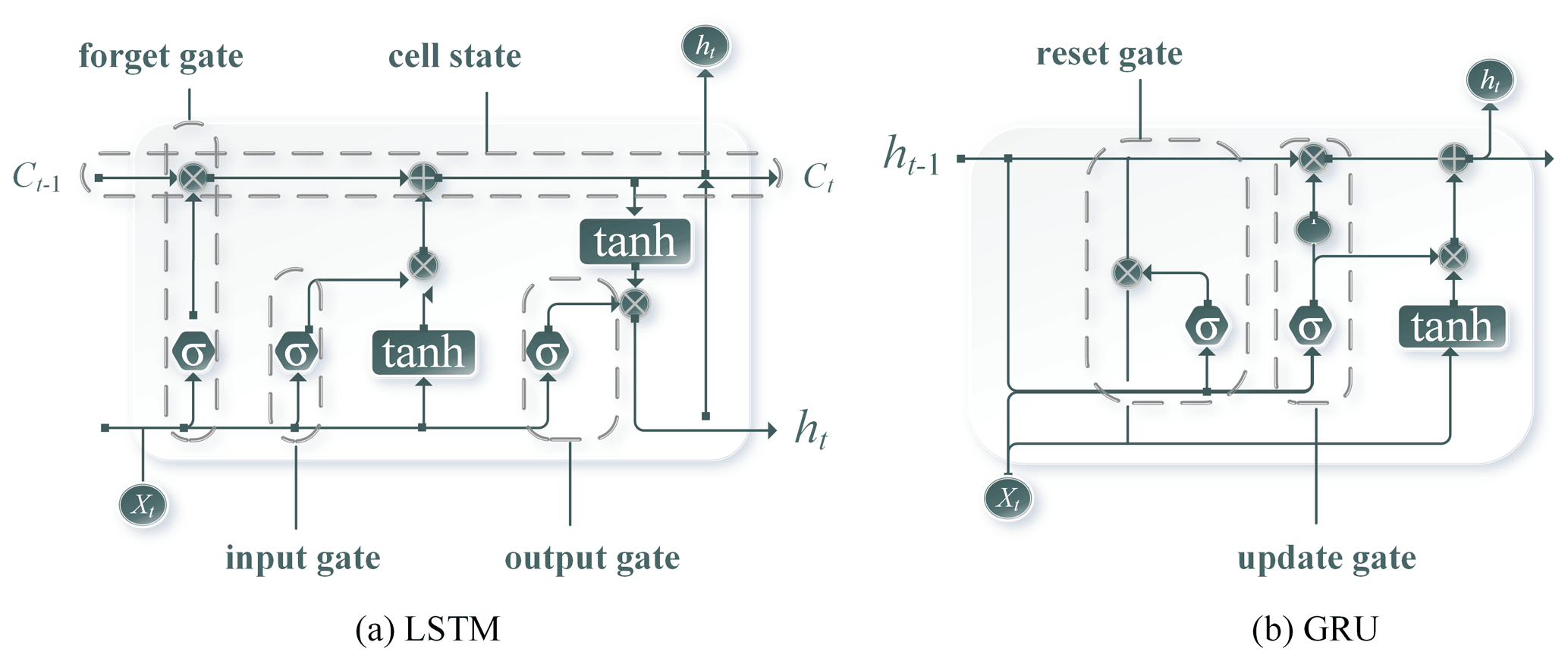
The LSTM network is one of the recurrent neural networks (RNNs) developed by Hochreiter and Schmidhuber (1997), and the basic structure of an LSTM cell is illustrated in Fig. 2a. It is an improved RNN aiming to solve problems such as gradients in long-term memory and backpropagation. The LSTM cell has three gates maintaining and adjusting its cell state and hidden state, including the forget gate, input gate, and output gate. The forget gate determines what information should be thrown away from the cell state. The input gate decides which information is used to update the cell state. The output gate controls which information stored in the current cell state flows into the new hidden state. In Fig. 2a, the state (ct) and the hidden state (ht) of the LSTM cell are updated as follows (Hochreiter and Schmidhuber, 1997):
where gt, ct, ot, and represent the forget gate, input gate, output gate, and potential cell state, respectively. ⊙ denotes the element-wise multiplication of vectors, and tanh(⋅) is the hyperbolic tangent. xt represents the current input vector, ht−1 denotes the last hidden cell state, and the initial state of ht is h0=0. σ(⋅) represents the logistic sigmoid function. [Wf, Wi, Wo, ], [Uf, Ui, Uo, ], and [bf, bi, bo, ] represent the input weight matrix, recurrent weight matrix, and bias vectors for the forget, input–output, and potential cell gates, respectively.
2.1.2 Gated recurrent unit (GRU)
GRU networks were proposed as a modification of LSTM networks with a more straightforward structure (Cho et al., 2014). The specific structure of the GRU cell is shown in Fig. 2b. Compared with LSTM, GRU only has two control gates, including a reset gate and an update gate. The update gate is applied to control how much information of the previous step is brought into the current step, while the reset gate is used to control the degree of ignoring the information of the previous state. In this way, GRU is superior to LSTM in terms of computer modeling time and parameter updates. In Fig. 2b, the state (ct) and the hidden state (ht) of the GRU cell are updated as follows (Cho et al., 2014):
where rt, zt, and represent the reset, update, and potential cell state, respectively. ⊙ denotes the element-wise multiplication of vectors, and tanh(⋅) is the hyperbolic tangent. xt represents the input vectors, ht−1 denotes the last hidden cell state, and the initial state of ht is h0=0. σ(⋅) represents the logistic sigmoid function. [Wr, Wz, ], [Ur, Uz, ], and [br, bz, ] represent the input weight matrix, recurrent weight matrix, and bias vectors for the reset, update, and potential cell gates, respectively.
2.1.3 Least-squares support vector machine with grey wolf optimizer (GWO-LSSVM)
LSSVM is a modified version of SVM, proposed by Suykens and Vandewalle (1999) to reduce the computational time of SVM. SVM uses the quadratic program to formulate the training process of the modeling procedure, while LSSVM aims to employ the least-squares loss functions. The LSSVM nonlinear function is expressed as (Suykens et al., 2002)
where φ(⋅) is the mapping function that maps the input x into a d-dimensional feature vector, w is a weight vector, and b represents bias. In LSSVM, a minimum objective function is proposed to estimate ω and b (Suykens et al., 2002).
that has the following constraints (Suykens et al., 2002):
where e is the error variable, and γ is the regulative constant. The objective function can be obtained to solve the optimization problems in Eq. (15) by introducing the Lagrange multipliers α and transferring the constraint problem into an unconstrained one (Suykens et al., 2002):
By finding the partial derivative of Eq. (16) with respect to w, b, αi, and ei, the following equation can be derived:
where K(x,xi) is the kernel function. Many kernel functions such as linear, polynomial, radial basis, and sigmoidal have been proposed for LSSVM (Bemani et al., 2020). We adopt the most widely used kernel function, radial basis function (RBF), in this study. The RBF is expressed as
where σ2 is the kernel parameter. In this study, the parameters γ and σ were optimized using the grey wolf optimizer (GWO). Please see more details on GWO in Guo et al. (2020d).
2.2 Bayesian model averaging (BMA)
Generally, it is difficult to determine which model is the best one, leading to model uncertainty. BMA is proposed to solve the uncertainty of the models through averaged estimations from individual models (Liu and Merwade, 2019; Samadi et al., 2020). The weight for each model is based on the simulated decision probability density function, i.e., the posterior probability of the model. Suppose Q is the unknown quantity we want to predict, given a subset of model forecasts , …, fK} (k=1, 2, …, K, where K is the number of individual model) and the observed data D, the posterior distribution of Q can be calculated as (Hoeting et al., 1999)
where is the posterior distribution of Q given the model forecast fk and the observed data D, and p(fk|D) is the posterior probability. In this case, posterior probabilities are the weighting factor for each model, and . The posterior mean (E) and variance (V) of Q are as follows (Hoeting et al., 1999):
where wk and are the posterior mean (weight) and variance of the kth forecast model. In this study, a log-likelihood function is maximized to estimate the parameters (weight wk and variance ) as shown in Eq. (21).
where θ is the vector of parameters {wk, , k=1, 2, …, K}. , is the Gaussian distribution function, where wk is the weight and is the variance.
The expectation–maximization (EM) algorithm (Lee et al., 2020) is used to find out the maximum likelihood with a termination criterion (early stopping or a maximal iteration). As the EM proceeds, the parameters of weight wk and variance are updated as follows.
where “Iter” is the number of iterations. NT is the length of calibration periods. Yt and are the observed and forecast streamflow at the tth time step, respectively (m3 s−1), and is the latent variable for the kth model at the tth time step in the Iter iteration. Then we use the Monte Carlo simulation method to generate BMA ensemble forecasts. Assume M is the number of Monte Carlo simulations, and the procedure is described below (Zhou et al., 2020a).
- a.
Set the initial cumulative weight , and calculate the cumulative weight for k=1, 2, …, K. Create a random variable u between 0 and 1. If , the kth forecast model would be used as the target forecast.
- b.
Generate a realization of the forecasts Qt using the Gaussian distribution function , . In such a way, there are a set of alternative forecasts to be chosen from as the final forecast.
- c.
Repeat steps (a) and (b) M times, and obtain a set of streamflow series . Furthermore, 90 % confidence intervals between the 5 % and 95 % quantities are employed to represent the uncertainty of BMA ensemble forecasts.
2.3 Forecast performance measures
Three performance indicators are applied to assess the deterministic forecast performance of the three data-process models. They are the Nash–Sutcliffe efficiency (NSE) (Nash and Sutcliffe, 1970), the root mean square error (RMSE) (Karunanithi et al., 1994), and the mean absolute error (MAE) (Legates and McCabe, 1999). They are expressed as below:
where T is the number of samples, Qm,t is the forecasted reservoir inflow (m3 s−1), Qo,t is the observed inflow (m3 s−1), and is the average of the observed inflow (m3 s−1). The NSE can be used to evaluate the stability of the forecasted value. In contrast, the RMSE and MAE are used to characterize the overall forecast accuracy. The NSE value is (−∞, 1], while MAE and RMSE values are (0, +∞). Generally, models with larger values of NSE or smaller values of RMSE and MAE provide better forecasting accuracy.
In addition, two performance indicators are used to evaluate the performance of ensemble forecast models, i.e., the containing ratio (CR), and average deviation amplitude (D), which were adopted for assessing the goodness of the prediction bounds (Xiong et al., 2009).
where and represent the lower and upper prediction bounds of streamflow (m3 s−1), respectively. Clearly, models with higher CR values but lower D values would produce better performance.
2.4 Parameterized multi-objective robust decision-making (MORDM)
This study proposes a parameterized multi-objective robust decision-making approach to design operating policies for the multi-objective reservoir operations by combining direct policy search (DPS) and multi-objective robust decision-making (MORDM). In the parameterized MORDM, instead of using the volumes of water to be allocated as the decision variables, we prescribe decisions approximated as nonlinear functions conditioned on system state variables (e.g., forebay water level observed or predicted inflows and precipitation) (Giuliani et al., 2016; Quinn et al., 2017a, b; Salazar et al., 2017). The nonlinear functions can be realized by the DPS approach. DPS is based on the parameterization of the operating policy pθ and the exploration of the parameter space Θ to find a parameterized policy that optimizes the expected function, i.e.,
where J1, J2, …, JM are the objective functions, and M is the number of objectives. is the corresponding optimal policy with parameters θ*. Different DPS approaches have been proposed, where two nonlinear approximating networks, namely artificial neural networks (ANNs) and radial basis functions (RBFs), have become widely adopted as universal approximators in many applications (Deisenroth et al., 2013). In particular, we parameterize the operating policy as RBFs because they have been demonstrated to be effective in solving multi-objective water resources management problems (Giuliani et al., 2014, 2015), and the kth decision variable in the vector ut (with k=1, …, K) is defined as
where N is the number of RBFs φ(⋅), Γt is the policy input vectors at the tth time step including exogenous information (e.g., forebay water level observed or predicted inflows and precipitation), and ωi,k is the weight of the ith RBF, . The single RBF is defined as follows:
where (Γt)j is the jth policy input at the tth time step, and M denotes the number of policy input vectors Γt, j=1, 2, …, M. ci and bi are the M-dimensional center and radius vectors of the ith RBF, respectively. The centers of the RBF must lie within the bounded input space (Yang et al., 2017). The parameter vector θ is defined as , where the number of θ is . In general, when DPS problems involve multiple objectives, they can be coupled with truly multi-objective optimization methods, such as multi-objective evolutionary algorithms (MOEAs), which allow for an approximation of the Pareto front in a single run of the algorithm.

In our study, the parameterized MORDM approach will be coupled with a rolling horizon scheme over a 1-year period to solve the multi-objective reservoir operation problem. Given the lead time of 7 d (the forecast horizon is equal to the operation horizon) as an example, it is operated following two steps: the optimization model is first operated daily over a 7 d horizon using the parameterized MORDM; after implementing current water allocation decisions, the status, inflow, and other information of reservoirs update as time evolves, and then the remainder is subsequently operated. The two steps are repeated until the process (1-year period) is completed. In each operating horizon, the main steps of the parameterized MORDM are described below and presented in Fig. 3.
-
Problems are formulated, including the performance measures and constraints.
-
Generate alternative parameterized policies subject to all the constraints, and the objectives are evaluated over stochastic inflows with the following procedures (Giuliani et al., 2016):
- a.
The operating policies are parameterized using RBFs.
- b.
Run a system simulation from t=1, 2, … 7 d upon each individual parameterized policy pθ for each inflow series and obtain the system trajectories.
- c.
Compute the parameterized policies performance in terms of the operating objectives as a function of system trajectories.
- a.
-
Recompute the parameterized policy performance with robust criteria, for instance, the principle of insufficient reason, minimax, and minimax regret (Guo et al., 2020b). Among them, the principle of insufficient reason transforming the problem under uncertainty into a decision-making problem under risk has been used in water resources problems (Giuliani and Castelletti, 2016). The principle of insufficient reason suggests that in the absence of knowledge on the probabilities associated with the different states, the decision could be taken by assigning equal probability to all the states (i.e., ). The robust parameterized policy performance can be expressed as
where Obj(pθ,sj) is the performance function using parameterized policy pθ upon jth streamflow series, sj denotes the scenario of the jth streamflow series, and n is the number of stochastic streamflow series.
-
Optimize the parameterized policies using multi-objective evolutionary algorithms (MOEAs) based on the robust performance objectives. Repeat steps (2)–(4) until the times of population iteration are reached, and export the optimal Pareto solutions. In this study, the optimization is solved by applying NSGA-II to search the space of decision variables and identify the trajectories.
It should be noted that the parameterized MORDM in this study aims to solve optimization problems under uncertainty, and thereby one streamflow series needs to be repeated multiple times.
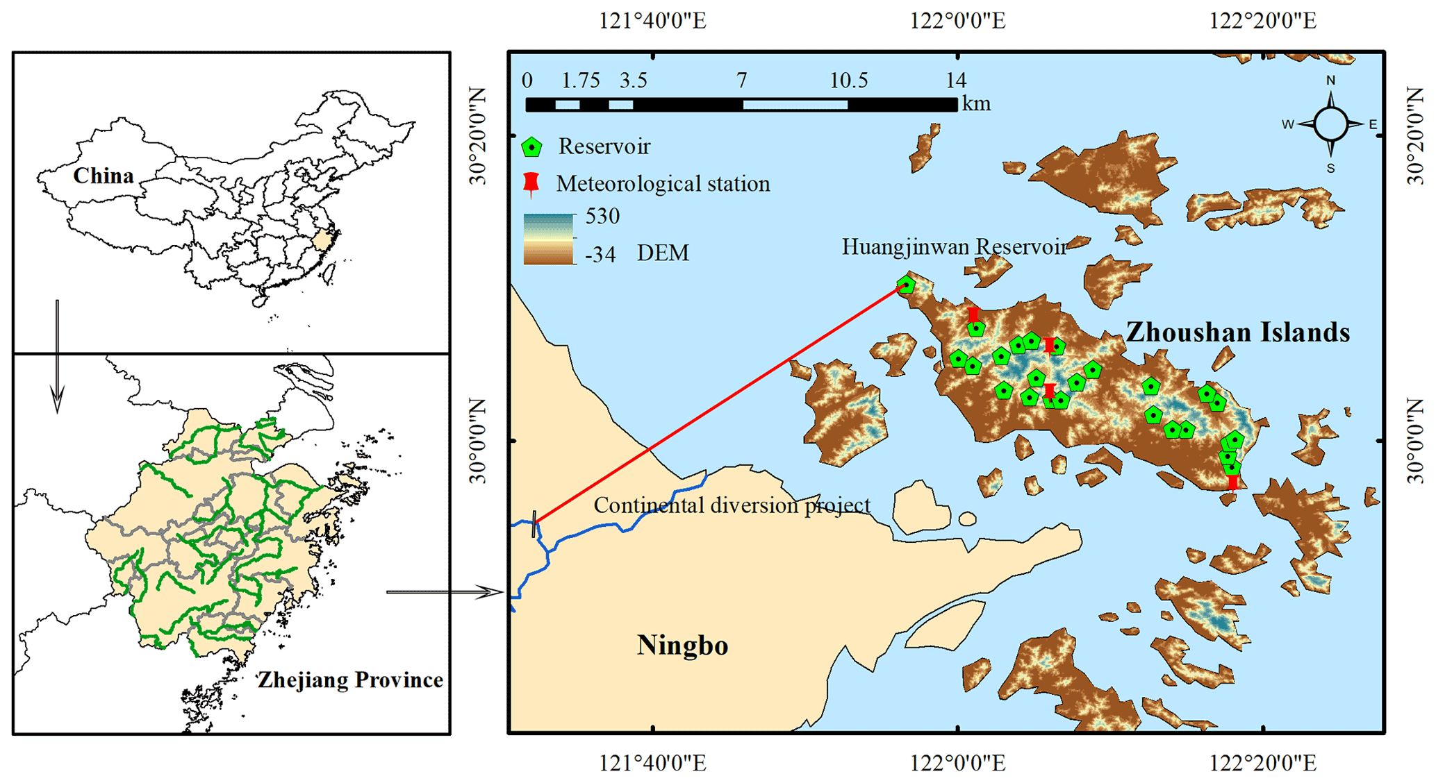
Figure 4Location of the Zhoushan Islands.
3.1 Study area and data
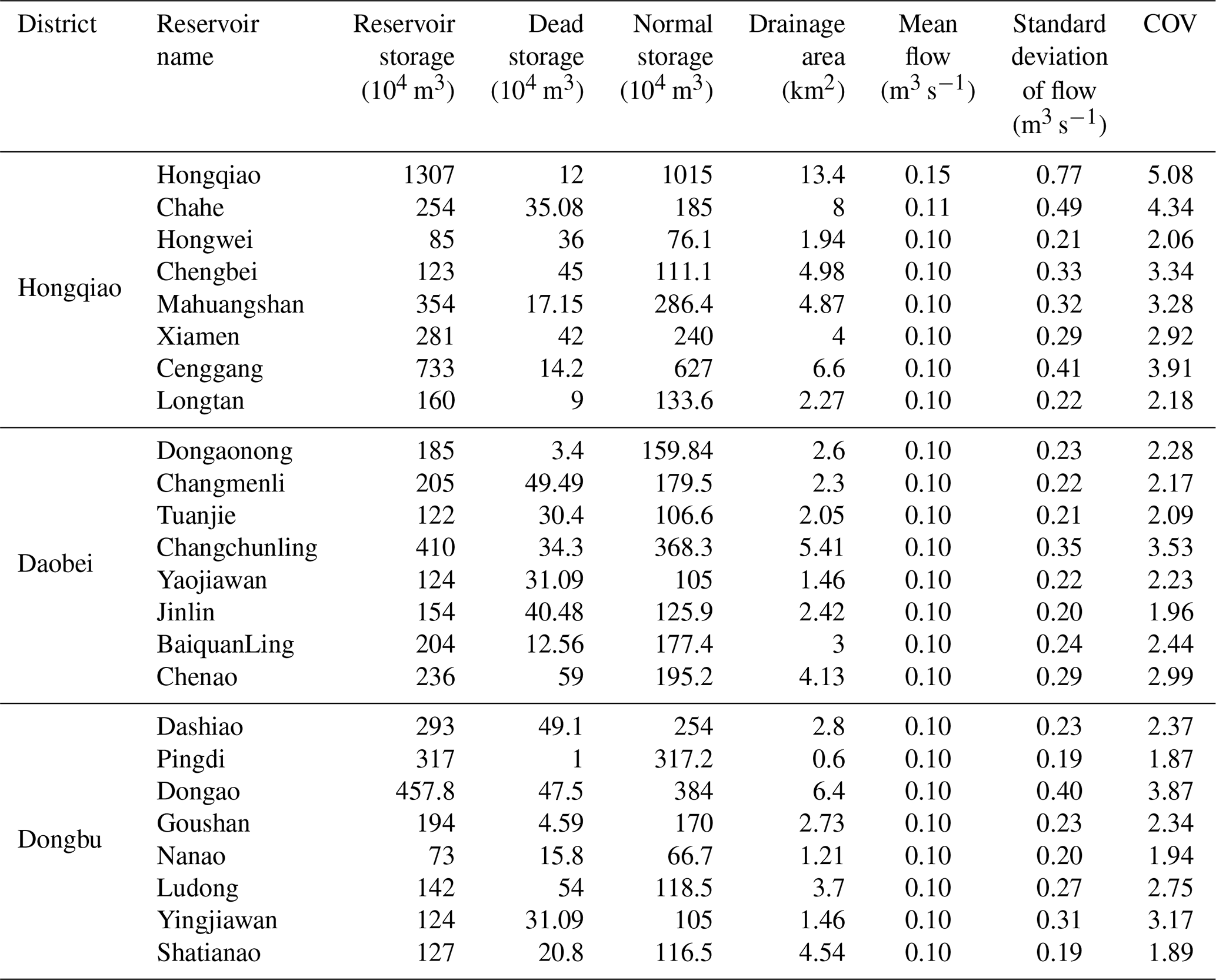
The Zhoushan Islands are located in the northeast of Zhejiang Province, China, with a total area of 22 000 km2 and 1390 islands (Fig. 4). The climate is governed by monsoon-influenced subtropical marine weather systems, and the annual mean temperature and precipitation are 17 ∘C and 1300 mm, respectively. There are no large rivers in the islands, and the insufficient freshwater resources severely limit the development of industry and population in the Zhoushan Islands. Recently, a continental diversion project transferring water from the city of Ningbo to Zhoushan Islands has been treated as an effective solution to overcome the water scarcity problem partially. The transferred water is stored in Huangjinwan Reservoir and then operated together with the limited freshwater resources in the remaining 24 reservoirs to supply water to four water plants, i.e., Daobei, Hongqiao, Lincheng, and Pingyangpu. Data for this study include historical inflow and state of reservoirs, water demand of water plants, and climate forcing data over 2002–2008. The climate data, including daily precipitation and evaporation, are observed at one meteorological station and three rainfall stations. The characteristics of the reservoirs are listed in Table 1.
3.2 Problem formulation
Figure 5 shows the simplified schematic diagram of the water supply system in Zhoushan Islands, including reservoirs, pumping stations, pipelines, and water plants. The pipeline arrow indicates the direction of the water flow. It covers the processes associated with water abstraction from resources, water distribution through the network involving the use of pumping stations and pipelines, and main activities relevant to water flow. In this study, water resources include local surface water and imported water. The surface water is the water stored in local reservoirs (a number of 24 reservoirs), while the imported water is the water transferred from the city of Ningbo (stored in Huangjinwang Reservoir). The imported water is transferred from the city of Ningbo to Zhoushan Islands through Lixidu and Lanshan pumping stations. End users within the water supply system are generally divided into the household, industry, agriculture, and environmental use. This study mainly considers household and industry use, which water plants can supply. The agriculture and environmental use are satisfied through operating the reservoir storage above a specific value. That is to say, the main goal of the water allocation plan is to ensure sufficient water flows into the four plants in Zhoushan Islands. They are Daobei, Lincheng, Hongqiao, and Pingyangpu plants, respectively. Releases from the reservoirs (Huangjinwan Reservoir and the remaining 24 local reservoirs) must meet the requirements of water plants. As observed in Fig. 5, the reservoirs supplying plants can be divided into two categories. Some reservoirs can directly release water into the plants or reservoirs, including Longtan, Ludong, Shatianao, Nanao, Chenao, Cengang, Tuanjie, and Changchunling reservoirs. In contrast, the other reservoirs can only release water into the plants or reservoirs using pumping stations. In such a way, the pumping flow can be obtained by summing reservoir releases through the corresponding pumping station, using the following equation.
where denotes the jth pumping flow at the tth time step (m3 s−1), denotes the release of the nth reservoir at the tth time step (m3 s−1), and N1 is the number of reservoirs pumped by the jth pumping station.

It can be noted in Fig. 5 that there are no specific hydraulic connections between most of the reservoirs, while Chahe, Hongwei, Chengbei, and Xiamen reservoirs can release water into Hongqiao Reservoir (the largest reservoir in Zhoushan Islands). With a water plant as a center, the whole islands are divided into four districts, i.e., Daobei, Lincheng, Hongqiao, and Dongbu. The dashed line represents the district boundary. Each district includes a water plant, several pumping stations, and reservoirs to supply water for the water plant. The hydraulic connection between such a water plant and corresponding pumping stations and reservoirs can be expressed as
where is the amount of water supply for a water plant at the tth time step (m3), J is the number of pumping stations flowing into the water plant, and N2 is the number of reservoirs directly releasing into the water plant.
In Fig. 5, every two system elements are connected by the pipelines, e.g., reservoir and reservoir, reservoir and pumping station, and pumping station and water plant. In some cases, more than one reservoir or pumping station share one pipeline, leading to competition on channel flow. However, the multi-objective optimization problem is operated on a daily time step in our study, and we assume reservoir releases or pumping station flows to the water plant without considering the channel flow limitation, thereby regardless of the specific hydrologic connections between channels or pipelines.
Three objectives are identified to evaluate the performance of the strategies. The conflicting objectives are to minimize the water deficiency ratio of the Daobei Plant, minimize the water deficiency ratio of the remaining three plants (Hongqiao, Lincheng, and Pingyangpu), and maximize the net benefits. The three plants can feed each other and thus are considered together in our study. A decision maker would consider a different suite of costs depending on whether an existing system is being managed or a completely new system is being designed. As water supply occurs in an existing system, costs considered in this study are the operating costs. These objective functions are given as follows:
where Obj1 and Obj2 are the water deficiency ratio of Daobei Plant and the sum of the remaining three plants, respectively (%); Obj3 denotes the net operating costs (RMB); and are the amount of water supply and demand for Daobei Plant at the tth time step, respectively (m3); and are the amount of water supply and demand for the kth plant (one of the remaining three plants) at the tth time step, respectively (m3); and are the operating costs for water supply using local reservoir water and imported water, respectively (RMB); and Mr is the revenue (RMB). The costs and revenue can be obtained according to the following:
-
operating costs for water supply using local reservoir water (, RMB),
where , , and represent the water resource fees paid to the government, water fees paid to reservoir managers, and the electricity fees in Zhoushan Islands, respectively (RMB); , , and denote the constant vectors, representing the unit price of water resources, water, and electricity in Zhoushan Islands, respectively (RMB per m3). Δt is the time step; i is the index of a reservoir; j is the index of a pumping station; I denotes the number of reservoirs; J denotes the number of pumping stations in Zhoushan Islands; denotes the amount of water supply for plants using local reservoir water at the tth time step (m3); denotes the supporting motor power of the jth pumping station (Kw); denotes the flow through the jth pumping station at the tth time step (m3 s−1); denotes the upper flow boundary of the jth pumping station in Zhoushan Islands (m3 s−1).
-
operating costs for water supply using imported water (, RMB),
where , , and represent the water resources fees paid to the government, water fees paid to the river managers, and electricity fees in the city of Ningbo, respectively (RMB); , , and denote the constant vectors, representing the unit price of water resources, water, and electricity in the city of Ningbo, respectively (RMB/m3); denotes the amount of water supply for plants using imported water at the tth time step (m3); denotes the flow through the jth pumping station at the tth time step, and J is the number of pumping stations transferring water from the city of Ningbo, J=2, . Lj denotes the length of the continental diversion pipeline using the jth pumping station (m), and denotes the upper flow boundary of the ith pumping station for water transfer (m3 s−1).
-
revenues (Mr, RMB),
where b denotes the unit price of water supply revenue (RMB per m3).
The optimization model is subject to the following constraints:
where It,i is the inflow of the ith reservoir at the tth time step (m3 s−1); Vt,i is the storage of ith reservoir at the tth time step (m3); Vmin and Vmax are the lower and upper storage boundaries, respectively (m3); is the maximum release of the ith reservoir at the tth time step (m3 s−1). In some cases, obtained by the RBF policies can be greater than , and we will do the following step to modify .
3.3 Model development
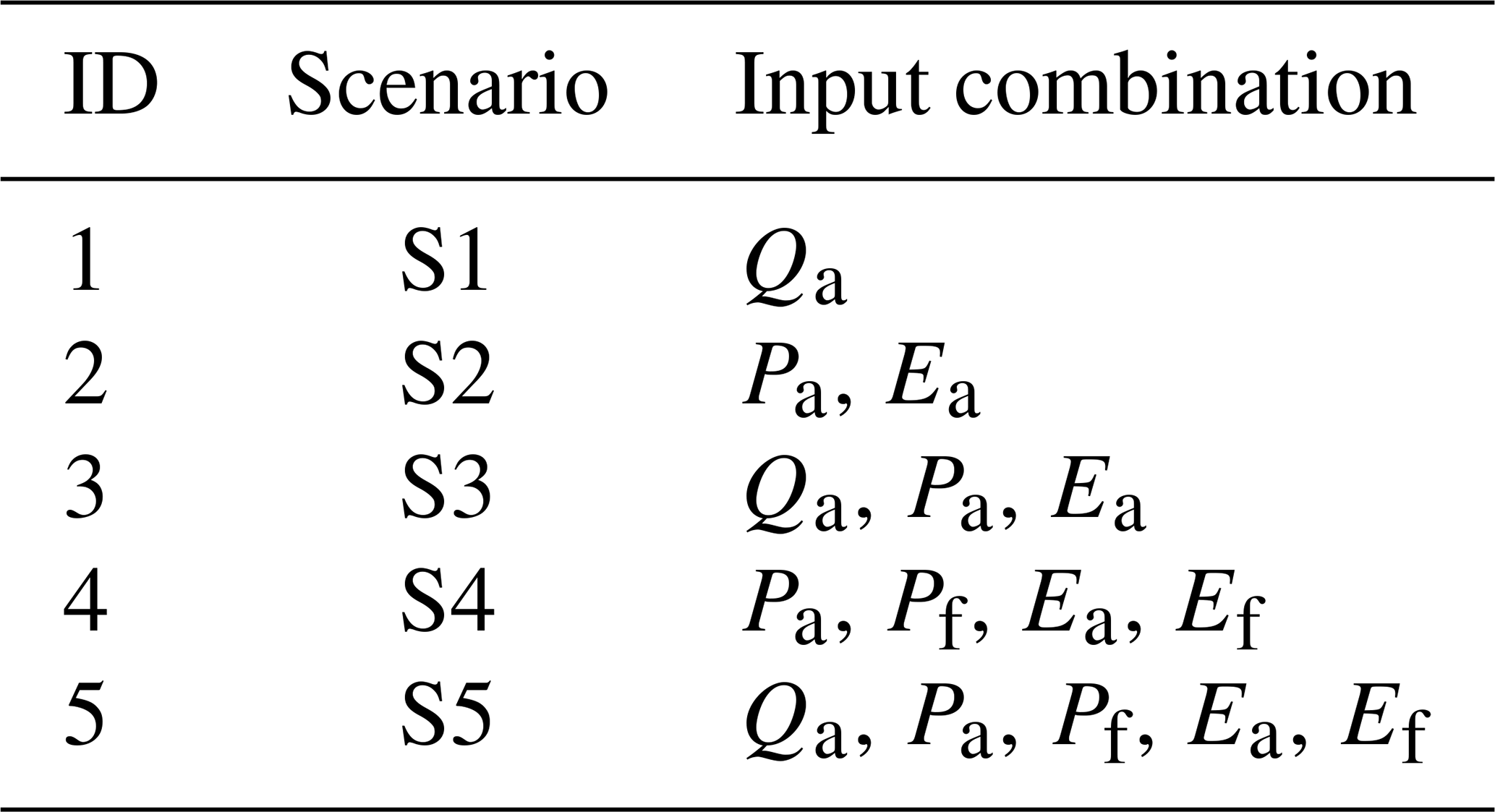
In this study, five input combination scenarios are considered to investigate whether the use of data-driven methods with climate forcing is efficient in inflow forecasts or not. These scenarios are described in Table 2. Pa represents antecedent precipitation, Ea represents antecedent evaporation, Qa represents antecedent streamflow, Pf represents forecast precipitation, and Ef represents forecast evaporation.
Several strategies have been proposed in the literature to tackle a multi-step-ahead forecast task (Kline, 2004), such as the recursive, direct combination of direct and recursive strategies. In this study, we chose one of the most carried out strategies, i.e., the direct strategy (Ben Taieb et al., 2012), to forecast multi-step streamflow over the short-term horizon (1–7 d). In this case, the streamflow is forecasted using the following equations, using S3 as an example.
where f(⋅) is the mapping function between inputs and outputs, which can be modeled by LSTM, GRU, and GWO-LSSVM in our case. The hydrological variables normalized to the same scale of [0, 1] are used as the inputs in the three ML methods. The normalization equation is given as follows:
where x and x′ are the original and normalized values, respectively. xmin and xmax are the minimum and maximum values of the original series, respectively.
An issue with the ML methods is that they can easily overfit training data. To avoid this, the entire data are divided into three subsets in RNNs: (i) a training set, which is used to compute the gradient and update the weights and biases of the network; (ii) a validation set, over which the errors are monitored during the training process and is used to decide when to stop training; and (iii) a test set, which is used to assess the expected performance in the future. In addition, dropout is a regularization method where input and recurrent connections to LSTM and GRU units are probabilistically excluded from activation and weight updates while training a network. The strategies mentioned above have the effect of reducing overfitting and improving model performance in RNNs. Both LSTM and GRU are trained based on truncated backpropagation through time (BPTT) (Cheng et al., 2020), which uses a backpropagation network to update the parameters in iterations. The NSE function is used as the loss function to calibrate the LSTM and GRU models. As for LSSVM, we avoid overfitting by minimizing the NSE during the calibration and validation periods, while the test period is also used to assess the performance. In this study, January 2002 to December 2006 is used as the training period, while the validation and tests extend from January–December 2007 and January–December 2008, respectively.
The multi-reservoir operation optimization using inflow forecasts is performed over 1 year (1 April 2007–31 March 2008) with 25 reservoirs. The period is selected to ensure that it does not cover the calibration datasets. For the short-term forecasting and reservoir operation purpose, a forecast horizon of 1–7 d ahead is chosen. In this study, we use the parameterized MORDM approach to design operating policies for the multi-objective reservoir operations under uncertainty. The optimized operations are regulated based on both deterministic and uncertain forecast inflow. To keep it fair, we perform a simulation to generate deterministic and observed ensemble forecasts, which are each repeated 900 times. Using the uncertain streamflow forecasts (BMA, deterministic or observed ensemble forecasts) as policy inputs in the parameterized MORDM method, we can generate alternative RBF policies that are subject to all the constraints, and the objectives are evaluated over stochastic inflows. Under the parameterized MORDM, the decision variables in the optimization problem are not the volumes of water to be transferred from the city of Ningbo and the remaining 24 reservoirs each day. Instead, the decision variables are the parameters of the RBF policies. The best operation is obtained by conditioning the operating policies upon the following two input variables, e.g., the initial forebay water level and current inflow of reservoir. The optimization is solved at each time step (a particular forecast horizon, e.g., 1–7 d) by applying NSGA-II to search the space of decision variables and identify the islands' water allocation trajectories.
3.4 Results and discussion
3.4.1 Multi-step deterministic forecasts based on ML methods
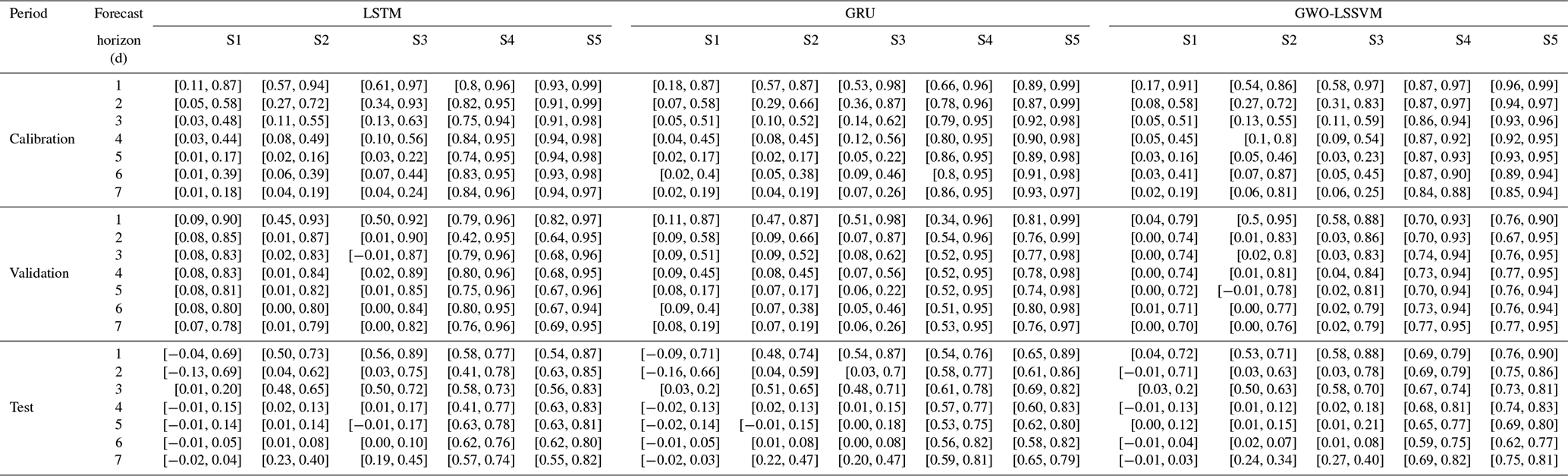
We consider five different input scenarios described in Sect. 3.3. Table 3 demonstrates the forecast analysis carried out with the different configurations (input combination and forecast model), tabulating the NSE ranges for lead times from 1 to 7 d ahead over all reservoirs during the calibration, validation, and test periods. It can be seen that S1 using only the flow variables and S2 using only the antecedent climate variables are inferior to the other scenarios. The performance is generally improved when the flow variables are used in combination with the antecedent precipitation and evaporation under S3. However, in this case, the antecedent variables succeed in forecasting only 1 d ahead. The forecast performance decreases significantly as the forecast horizon increases from 1 to 7 d ahead. Herein, we suppose that the following precipitation and evaporation have been forecasted. It is clear that S4 and S5, with the forecast climate variables, make significant increments in streamflow forecasting. The NSE can remain relatively stable at different horizons. There are no apparent differences between the three forecast models during the calibration period. However, the two RNNs perform better than GWO-LSSVM during the validation period, while GWO-LSSVM outperforms during the test periods. Besides, given that GRU has more superficial structures and fewer parameters and requires less time for model training, it may be the preferred method for short-term streamflow forecast compared with LSTM. The same results have been obtained in Gao et al. (2020) when they used LSTM and GRU to model short-term rainfall–runoff relationships.
Table 3NSE ranges ([min, max]) for all reservoirs with the different configurations during the calibration, validation, and test periods.
We aim to compare how the forecasted climate variables impact the streamflow forecast and reservoir operation performance. For the sake of brevity, S3 and S5 are compared in detail in the following section. Recall that S3 uses flow variables, antecedent precipitation, and evaporation as inputs, while S5 uses flow variables as well as the antecedent and forecast climate forcing. After assessing model validity, the next step is to compare the performance across the 24 reservoirs. The coefficient of variation (COV), defined as the ratio of the standard deviation of the inflow time series, is used to capture the varying characteristics of the incoming flow into the reservoir. Figure 6 reveals a strong negative relationship between COV and forecast performance under S3 at all lead times. The forecast performance decreases as the COV increases for all forecast models. This indicates that the more variation the flow has, the harder it is for data-driven methods to learn the flow pattern when there is not enough input information. However, the negative signal under S5 (Fig. 7) with forecasted climate variables (precipitation and evaporation in this study) is not as strong as that under S3, indicating that the forecast climate variables can help AI-based models' mapping functions between inputs and outputs. The improvements are more significant for the two RNN models, i.e., LSTM and GRU, than LSSVM. This result demonstrates that the efficiency of deep-learning RNN methods is better and more accurate than LSSVM.

Figure 6NSE values at lead times of 1 to 7 d plotted against the coefficient of variation (COV) for all the 24 reservoirs during the period of (a) calibration, (b) validation, and (c) test under S3.
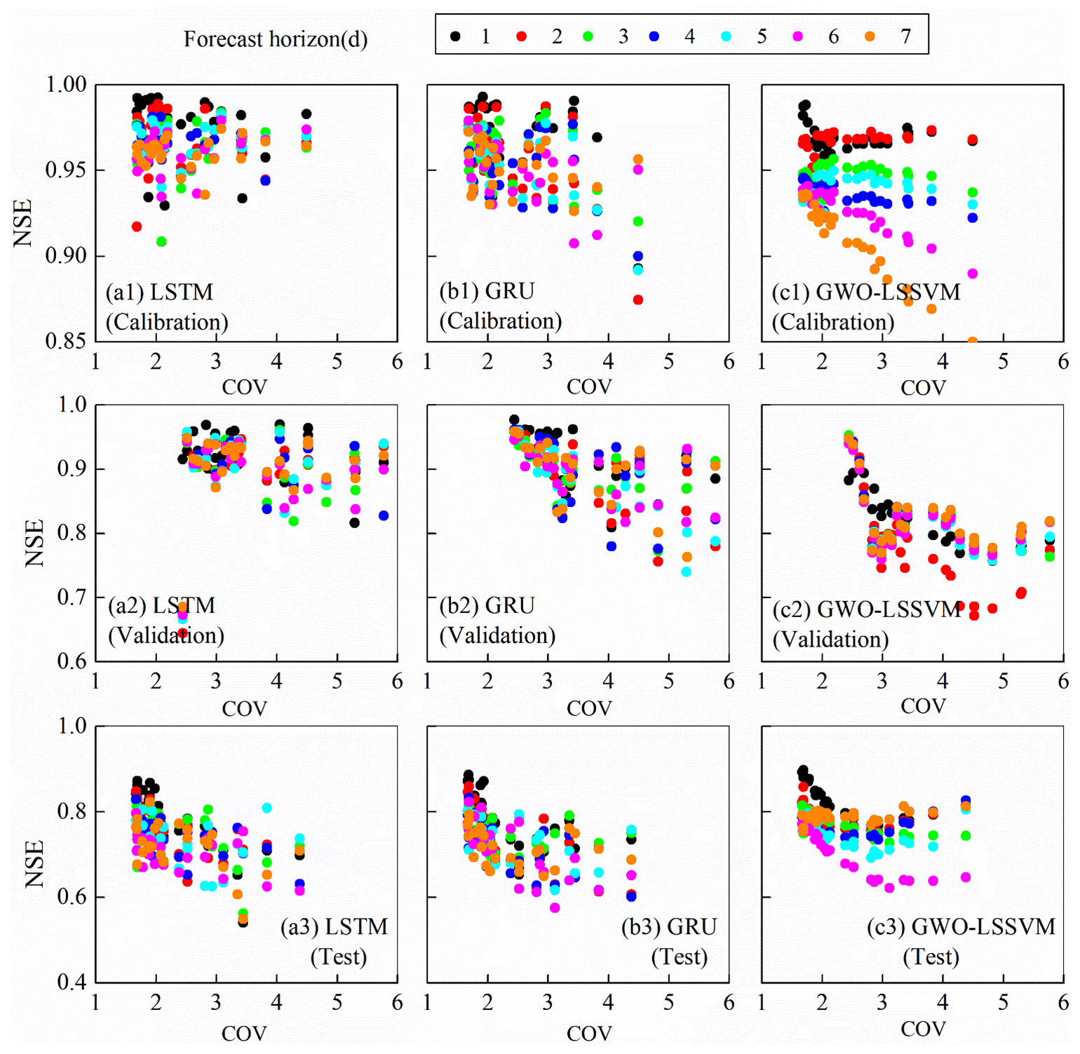
Figure 7NSE values at lead times of 1 to 7 d plotted against the coefficient of variation (COV) for all the 24 reservoirs during the period of (a) calibration, (b) validation, and (c) test S5.
3.4.2 Multi-step stochastic forecasts based on BMA method
Based on the forecast results of three data-driven models in the calibration period, the BMA method determines weights for LSTM, GRU, and GWO-LSSVM models. The weights reflecting the performance of the ensemble models during the calibration period are shown only for lead times of 1 and 7 d for the sake of brevity under S3 and S5 in Fig. 8. The model weights reflect the comparative importance of all the competitive modeling predictions on one level. Figure 8 indicates that it is difficult to conclude which individual model provides the best prediction. For example, GRU outperforms the remaining two models for Hongqiao Reservoir, while LSTM performs best for Cenggang Reservoir in Fig. 8a1. Similar results can be obtained from Fig. 8b1. Comparatively, Fig. 8a2 shows that LSTM and GWO-LSSVM influence the BMA model more than GRU. This higher weight is assigned because the forecasts are more similar to observations than those less similar to observations using the BMA posterior processor. However, observed from Fig. 8b2, the prediction accuracy of GWO-LSSVM is seriously affected and much less than that of GRU. It is consistent with the results obtained in Fig. 7, indicating that RNNs outperform GWO-LSSVM when there is more input information under S5. Overall, model uncertainty always exists whether forecast climate variables are involved or not, and it is necessary to analyze and evaluate the model uncertainty involved using BMA.
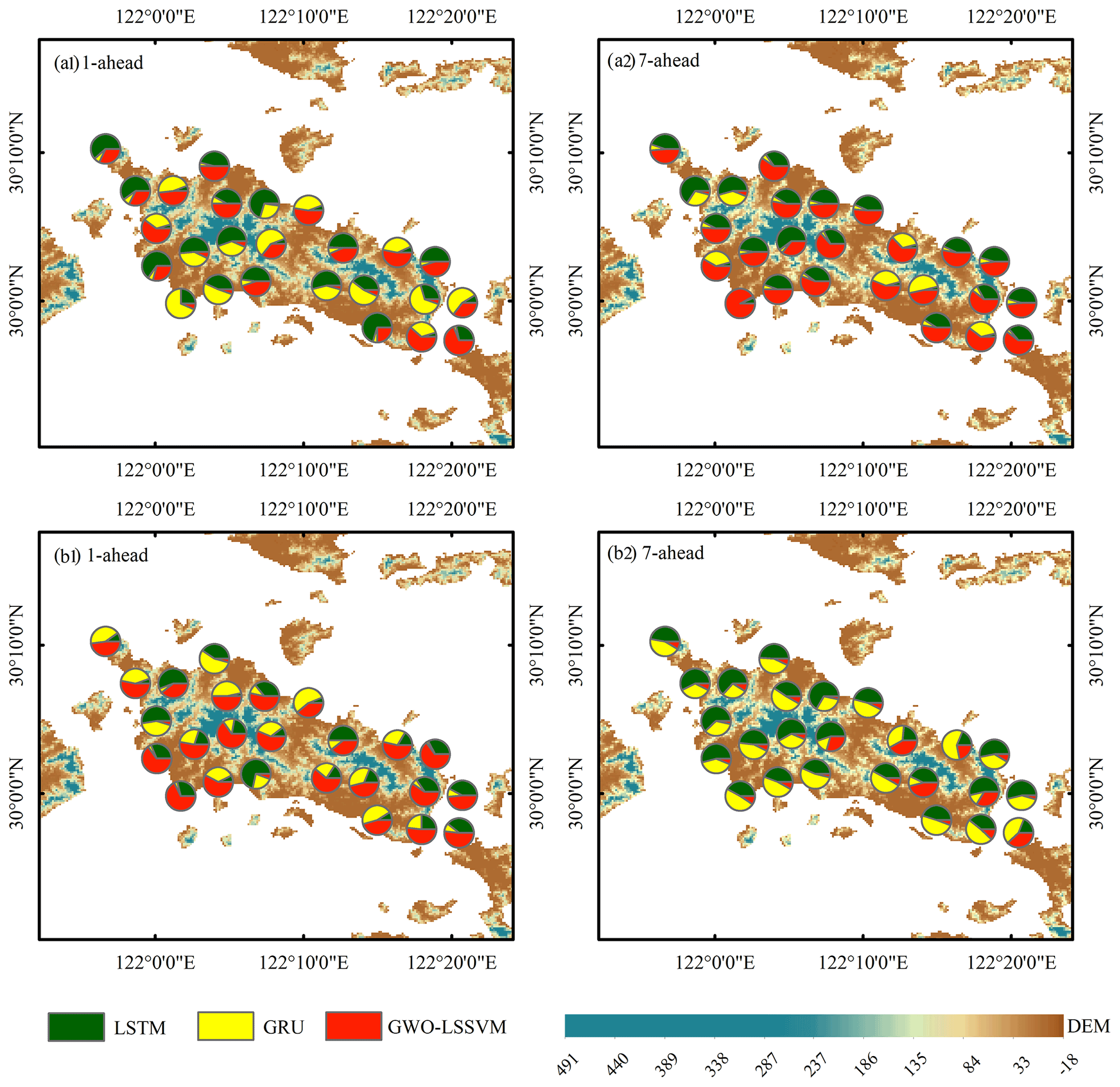
Figure 8Weights of three individual forecast models for the BMA model for all reservoirs under (a) S3 and (b) S5.
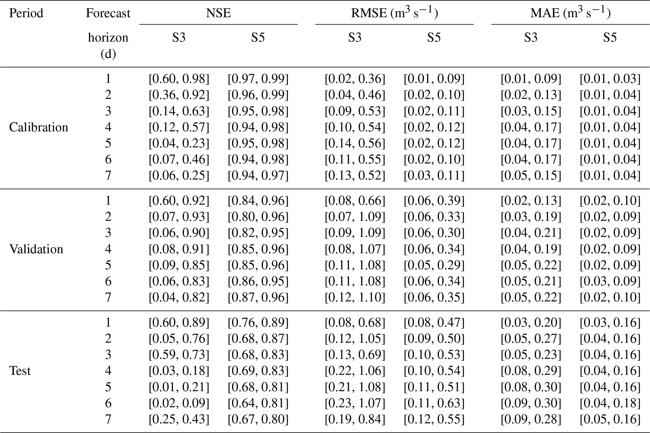
To access model validity, the evaluation of the modeled streamflow is performed over calibration, validation, and test periods using NSE, RMSE, and MAE metrics. Table 4 shows the performance metric ranges for all 24 reservoirs of BMA methods under S3 and S5. Apparently, both the replicative (forecast performance in calibration sets) and predictive (forecast performance in validation and test sets) validity under S5 for forecast horizons are significantly better than those under S3. For example, Fig. 9 demonstrates the improvement rates in terms of NSE, RMSE, and MAE of the BMA model compared with the three individual models. BMA produces the maximum NSE, minimum RMSE, and minimum MAE during the calibration period for both two scenarios, indicating that BMA has the best goodness of fit. This is because the weights are derived according to the individual forecast model in this period. With respect to validation and test periods, the BMA method shows better forecasts than the three comparative models except for the GRU modeling validation datasets under S5. Thus, it is shown that the BMA model matches the actual streamflow well.
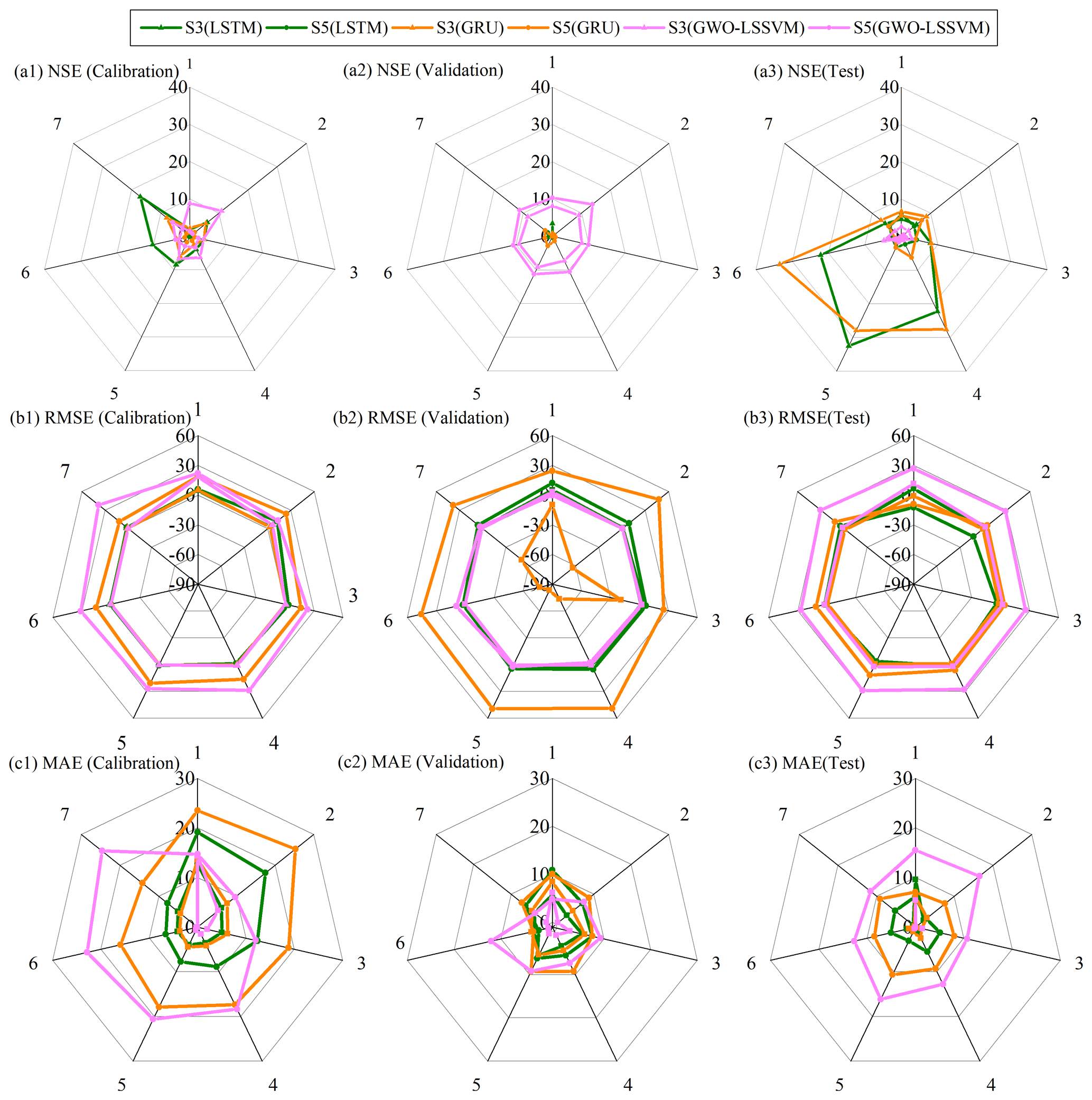
Figure 9Improvement rates in terms of averaged (a) NSE, (b) RMSE, and (c) MAE of the BMA model for forecasts as compared with the three individual models.
Table 4Performance metric ranges ([min, max]) for all 24 reservoirs of BMA methods under S3 and S5.
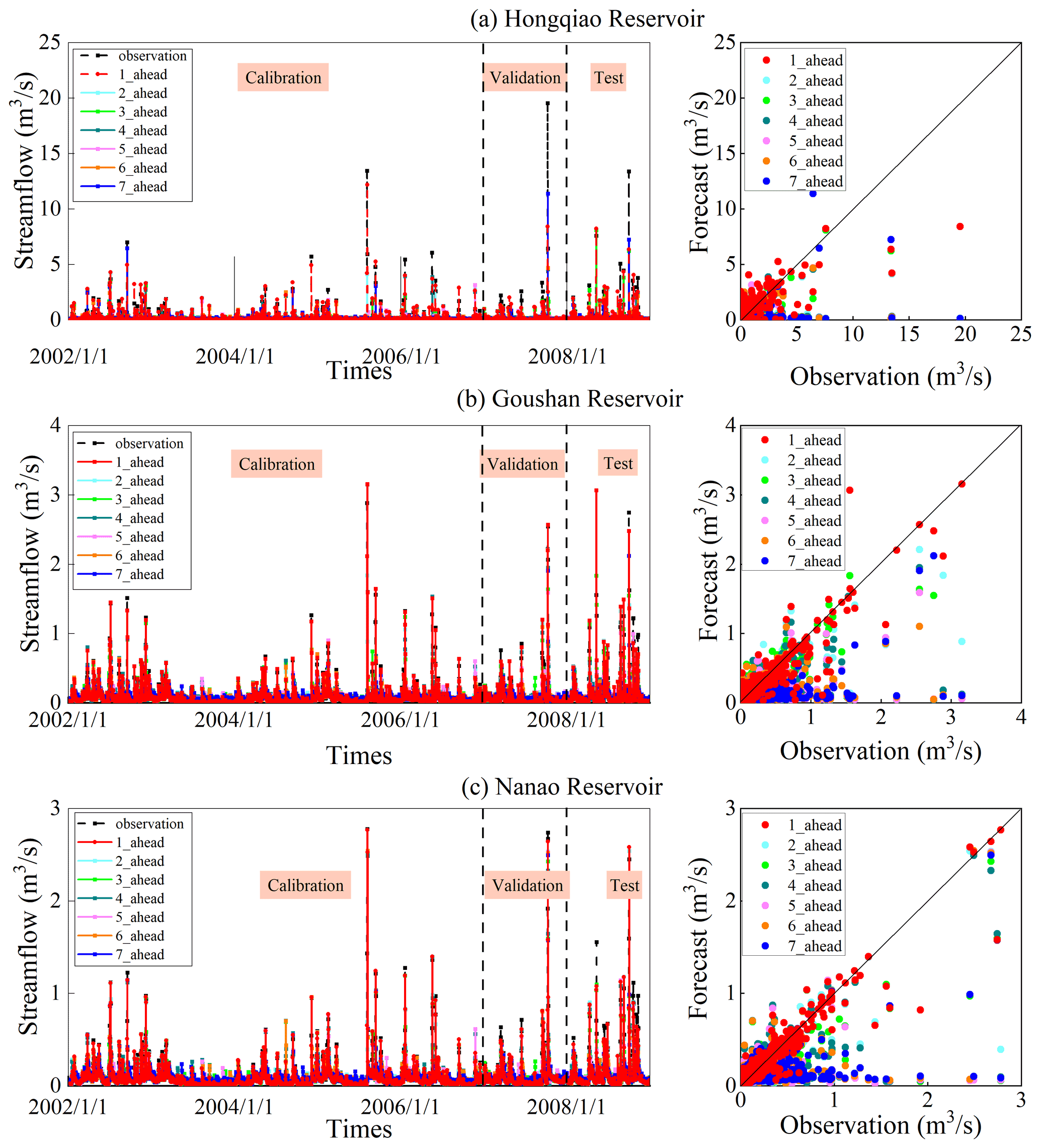
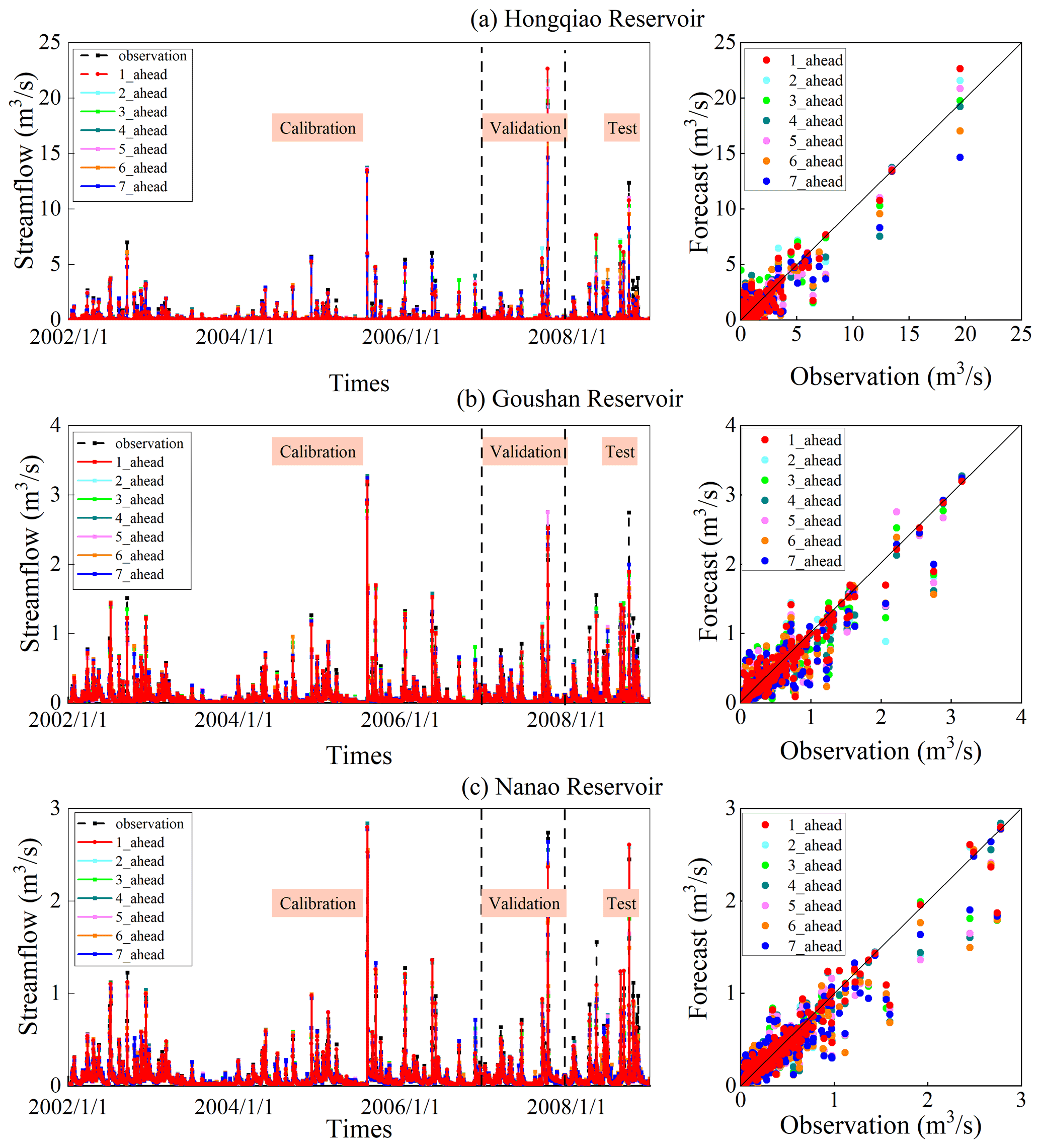
The model validity is then assessed using (i) hydrographs and (ii) scatter plots of observed and modeled streamflow, as shown in Figs. 10 and 11. Herein, we only show three reservoirs, i.e., Hongqiao (the largest reservoir), Goushan (the medium reservoir), and Nanao (the smallest reservoir), for the sake of brevity. From Fig. 10, it is clearly shown that the modeled streamflow deviates gradually from the 1:1 line, and the forecast skill decreases with the increase of lead time under S3 as expected, which is consistent with the statistical results shown in Table 4. In contrast, the scatters of the observed and modeled streamflow implemented with forecasted climate variables fit well across the 1:1 line at different lead times under S5, observed from Fig. 11. The performance for Hongqiao Reservoir is affected explicitly by an extreme peak event that hit the reservoir during the calibration period shown in Fig. 10, which does not occur over the training set of data. This causes heavy underestimations in the streamflow forecast. A more extended calibration period is required to improve the performance over such extreme peak flow events. However, the BMA method performs well on this extreme peak flow in Hongqiao Reservoir at all lead times when the forecast climate forcing is applied as inputs. This is because the reservoirs in Zhoushan Islands have relatively small drainage areas, and thus the flow is concentrated in a very short time after an extreme rain event.
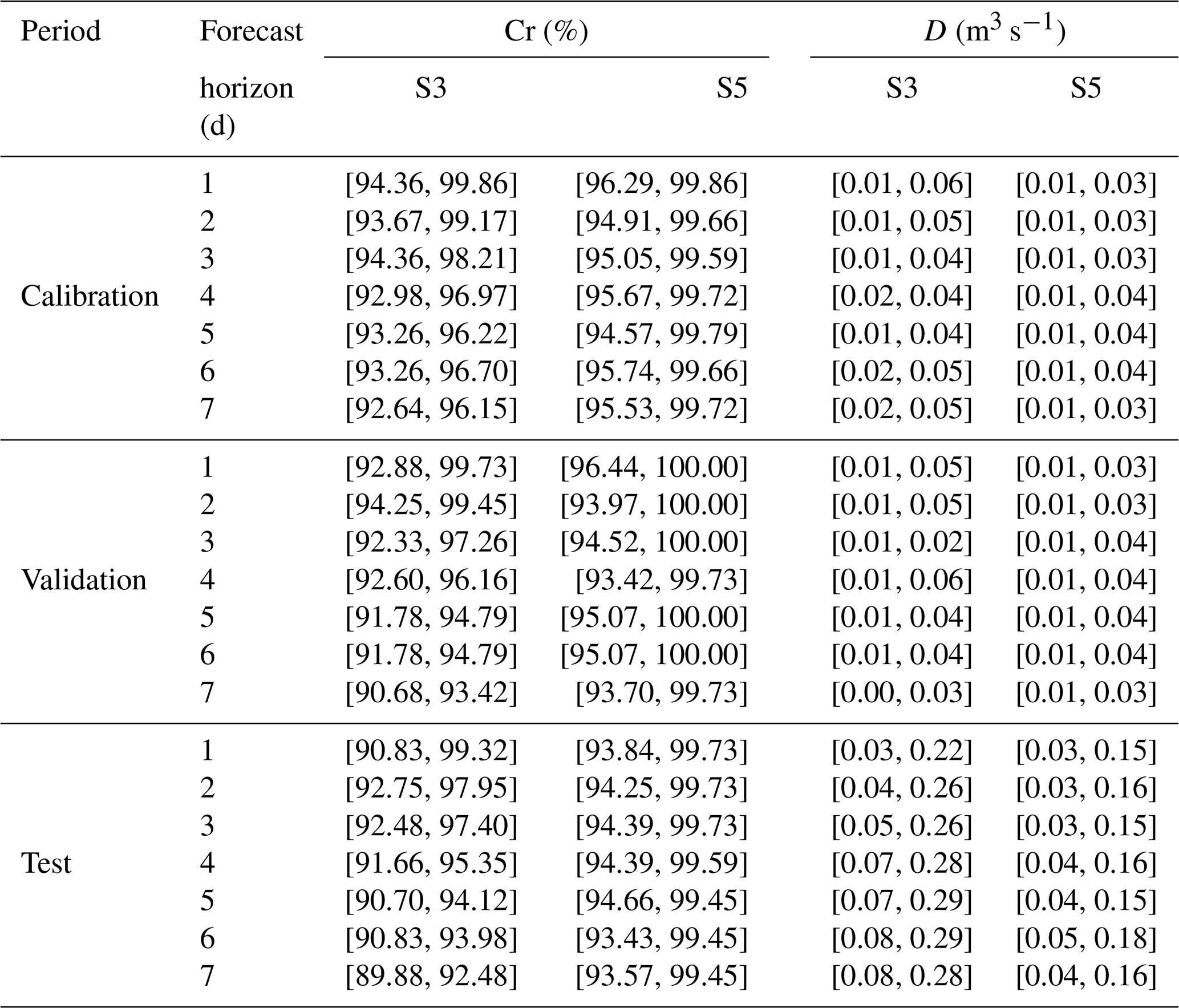
We use the Monte Carlo simulation method to generate BMA ensemble forecasts. The number of simulations is set as 1000 in this study. To demonstrate the optimization results of multi-reservoir operations based on the data-driven forecast models under uncertainty, 90 % confidence intervals associated with the deterministic predictions at BMA are further calculated. The confidence interval provides more alternatives that are possibly useful for a tradeoff between multiple objectives, such as flood control, hydropower generation, and improved navigation (Zhang et al., 2015). The interval performance metrics of Cr and D described in Sect. 2.3 are adopted to assess the performance of uncertain forecasts. Table 5 displays the averaged metrics for all the 24 reservoirs under S3 and S5. Both indicators under S5 are superior to those under S3. The 90 % streamflow interval between the 5th and 95th percentiles of some representative reservoirs, e.g., Hongqiao, Goushan, and Nanao reservoirs, are presented in Figs. 12 and 13. The results are consistent with those in Figs. 10 and 11. It is observed from Fig. 12 that the streamflow interval fails to capture the extreme peak flow for Hongqiao Reservoir under S3. The BMA performs gradually worse with increasing lead times for the three reservoirs. However, in Fig. 13, the red dots represent the observed streamflow, most of which are covered by the 90 % interval at both 1 and 7 d ahead. Therefore, the forecast climate variables will be conducive to reducing the predictive uncertainty of real-time streamflow forecasting.
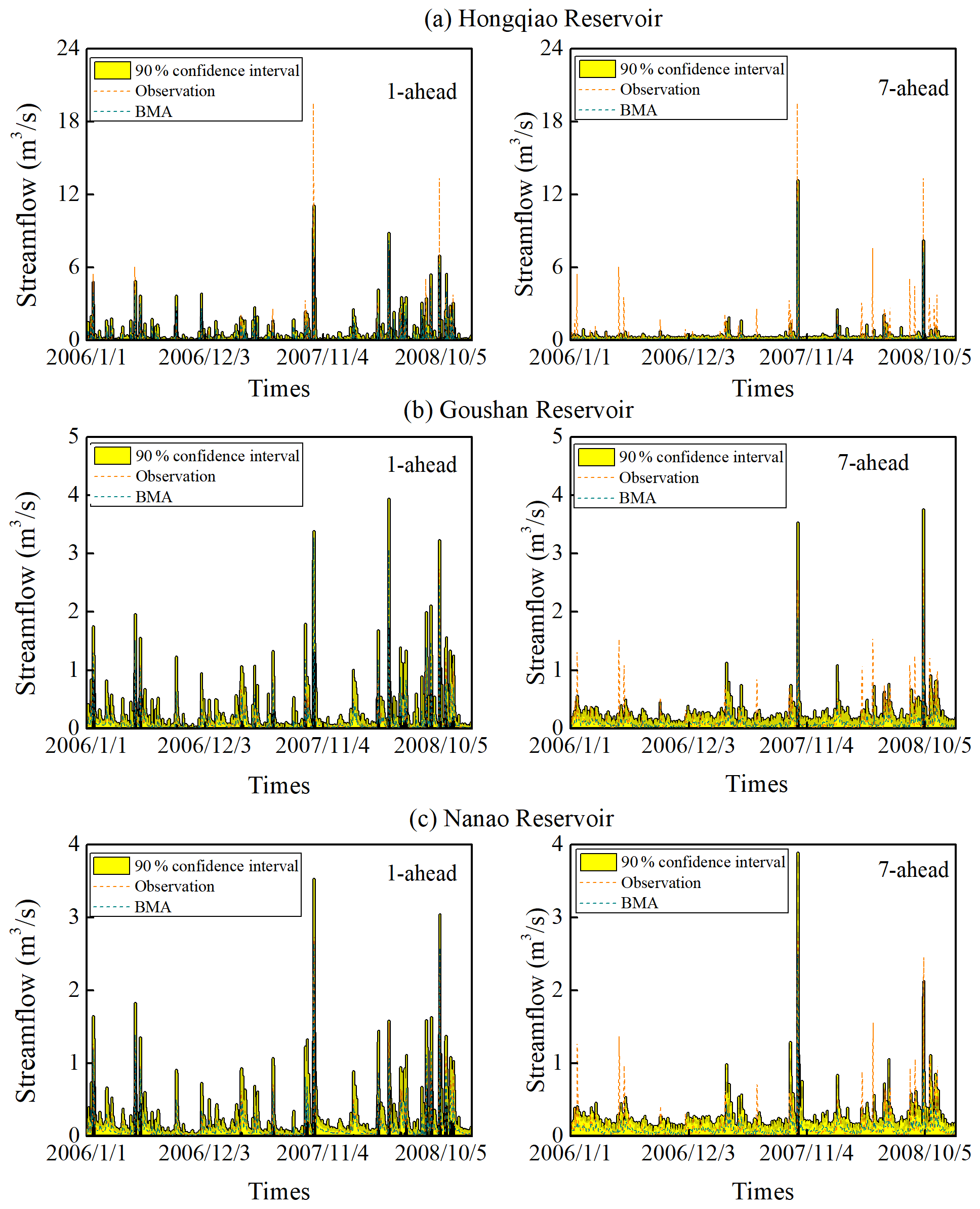

Table 5Ranges of interval performance metrics ([min, max]) for all the 24 reservoirs under S3 and S5.
3.4.3 Multi-objective reservoir operation performance evaluation
The optimized operations are regulated based on both deterministic and uncertain forecast inflow. To demonstrate the relationship between the conflicting objectives, a set of Pareto solutions over a 7 d horizon at different periods under S5 is given as an example, as shown in Fig. 14. The optimization using the Pareto concept allows the operator to choose an appropriate solution depending on the prevailing circumstances and analyze the tradeoff between the conflicting objectives. In each of the plots, the water deficiency ratio of Daobei Plant and the sum of the remaining plants are plotted on the x and y axes, respectively. The color of the markers indicates the net operating costs, with colors ranging from red, representing low value, to blue, representing high value. Thus, an ideal solution should be located at the left corner (low value of the water deficiency ratio of Daobei Plant and the sum of the remaining three plants) of the plot and represented by a red (low net operating costs) marker. The black arrows have been added in the figure to guide the reader in understanding the directions of optimization. Generally, the water deficiency ratio of Daobei Plant has an inverse relationship with that of the sum of the remaining plants (inverse relationship; i.e., the former decreases with the increase of the latter). In contrast, the water deficiency ratio of the remaining three plants has a positive relationship with the net costs (positive relationship; i.e., the former increases with the increase of the latter).

Figure 14A set of Pareto solutions at different periods over a 7 d horizon under (a) deterministic and (b) uncertain forecasts.
It is interesting to compare the performances associated with deterministic and uncertain forecasts. Uncertain conditions (Fig. 14b) show a much broader scale on the three objectives than deterministic conditions (Fig. 14a). For instance, uncertain forecasts produce the water deficiency ratio of Daobei Plant, ranging from −40 % to 80 %, during 12 to 18 August 2007, while deterministic forecasts have a smaller range, with a value from 30 % to 100 %. The water supply deficits under deterministic forecasts are due to the high demand happening in August, which can be mitigated when informing the reservoir operations with uncertain forecasts. In this way, we expect that if the ensemble streamflow forecasts are used in a stochastic optimization scheme, the reservoir operation could be further enhanced because the optimization considers possible uncertainty provided by uncertain forecasts and thus takes advantage of correcting the influences of uncertainty.
-
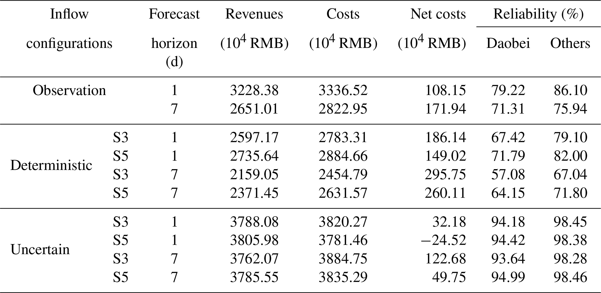
Performance evaluation with different forecast skills. In general, forecasts are always useful for reservoir operations. The annual revenues, costs, and water supply reliability are chosen as metrics to compare the performance of the operating policies derived from different configurations. Reliability is a measure of how well the water demand for users is met in a water transfer system. In this case, reliability is expressed as a percentage. The system performances are averaged over a set of solutions. The annual values during the period from 1 April 2007 to 31 March 2008 at various configurations are provided in Table 6 with two decision horizons of 1 and 7 d. The multi-reservoir operation based on observation is designed as a benchmark. It can be seen from Table 6 that the performance indicators from the 1 d forecast horizon are better than those from 7 d using deterministic inflows (in the case of observed and forecasted inflows). Two scenarios (S3 and S5) with the 1 d forecast horizon show similar operating performance, which is consistent with the performance of the inflow forecast listed in Table 3. Recall again that S3 uses flow variables, antecedent precipitation, and evaporation as forecast inputs, while S5 uses flow variables as well as the antecedent and forecast climate forcing. In contrast to S3, the operating results of S5 with a 7 d forecast horizon are closest to that of the observation. This is due to the improved inflow forecast performance under S5. However, it is depicted in Table 6 that the indicator of water supply reliability and net costs under S5 are inferior to those under S3. As for the stochastic forecasts, S5 outperforms S3 with lower net costs and approximate water supply reliability. In this case, the improved performance may not lead to improved decisions in deterministic forecasts.
The results obtained in Table 6 show that system performance derived from the observed inflows is inferior to that from other configurations. This finding cannot confirm the effectiveness of inflow forecasts. The reason for that is the forecast inflows may overestimate the actual inflows. For example, the mean value (0.14 m3 s−1) of the observed inflow of Hongqiao Reservoir is lower than that of the forecasted inflow (0.17 m3 s−1). In this case, the good performance presented in Table 6 is “fake”. That is to say, although decision makers can follow the strategies determined by the forecasted inflows, the system performance should be assessed using the actual inflows (i.e., observed inflows). We further re-evaluate the operating strategies optimized from different configurations mentioned above using the observed inflows. The performance metrics are listed in Table 7. It is expected that the results can reveal the maximum efficiency and reliability that could be achieved based on accurate information. In general, the indicator values under deterministic forecasts in Table 7 are reduced compared with those in Table 6. The reason is that reservoir operating decisions in Table 6 are optimized based on a higher inflow series.
In terms of both deterministic and uncertain forecasts, net operating costs of S5 are improved significantly compared with that of S3, while water supply reliability is increased slightly. This result may suggest that improved forecasts are more skillful in making decisions when using forecast climate variables as inputs. We highlight that this result we obtained is specific to the Zhoushan Islands. Indeed, many studies show that higher forecast performance did not lead to better operation decisions (Chiew et al., 2003; Goddard et al., 2010; Turner et al., 2017). However, some researchers draw the same conclusions as us. For instance, Anghileri et al. (2016) declared that inflow forecasts with accurate weather components would produce much smaller water supply deficits. Moreover, Anghileri et al. (2019) found that preprocessed forecasts (higher performance) were more valuable than the raw forecasts (less performance) regarding two operation performance metrics, i.e., mean annual revenues and spilled water volume.
There is also an interesting finding that the operating performance upon deterministic forecasts deteriorates, while the performance upon uncertain forecasts can stay relatively stable. This implies that the use of uncertain forecasts in reservoir operation can be more efficient and reliable than that of deterministic forecasts. The reason is that in a stochastic optimization scheme, the value can be further enhanced because the optimization can account for the total uncertainty provided by the ensemble forecasts. Similar results were obtained by Roulston and Smith (2003), who reported that the hydroelectric power production derived from the ensemble forecasts was increased compared with the deterministic forecasts. Boucher et al. (2012) also found that stochastic forecasts outperformed deterministic ones with the lower turbinate flow, higher generation production, and less spillage during a flood period. Overall, in most cases, a noticeable improvement can be achieved through the use of the stochastic decision-making assistance tool.
We then assess the performance metrics of water supply reliability over different seasons. It is noted in Fig. 15 that the deterministic forecasts are less skillful than the uncertain forecast when used in spring (JFM), summer (AMJ), autumn (JAS), and winter (OND) with the two forecast horizons. Although the operating performance using the deterministic forecast is lower due to its deterministic character, the main characteristics of the relationship between the forecast quality and value remain unchanged. That is to say, the benefits of considering the forecasts are more significant when the forecast quality is higher. It indicates that the optimization is capable of exploiting efficient information to improve reservoir operations. In our multi-objective optimization modeling, we would like to make the best use of water resources and maximize water supply. However, the operating performance in autumn shows a lower value with respect to that in other seasons. This is because the water demand in autumn is usually much higher. The shortage does not imply the non-effectiveness of our proposed forecast-based management framework but is due to the limitation of available water and pumping station capacity.
-
Performance evaluation with different forecast horizons. The impact of different forecast horizons on the operation performance is further evaluated under different configurations, as shown in Fig. 16. It is noted that the operating policy optimized from uncertain forecast inflows upon S5 outperforms that from S3. In terms of deterministic conditions, S5 improves the operation on the metrics of water supply reliability of Daobei Plant, water supply reliability of the other plants, and net costs with a variation of 2.11 %–13.58 %, 2.74 %–7.38 %, and −19.94 % to −10.30 %, respectively, compared with S3. As for uncertain conditions, S5 improves by 0.24 %–1.90 %, 0.06 %–1.32 %, and −59.45 % to −176.19 %, respectively. Although the increments in water supply reliability are not insignificant, S5 can secure water demand with much lower operating costs than S3, which decision makers value most. Furthermore, uncertain forecasts produce an improved ratio of 31.52 %–65.01 %, 19.98 %–46.60 %, and −116.45 % to −56.95 % than deterministic forecasts regarding the three metrics, respectively. Our results again highlight that uncertain forecasts are more valuable than deterministic forecasts when designing forecast-informed reservoir operations.
With an increase in forecast horizon from 1 to 7 d, the performance in water supply reliability and net operating costs upon deterministic conditions are generally reduced. This suggests that considering a longer forecast horizon (up to 7 d) does not necessarily improve reservoir operation without future forecast climate variables as inputs (low forecast quality). The reduced performance in water supply reliability might be due to the fact that the optimization explores strategies to secure the whole water demand in a longer horizon, which results in a sacrifice in reliability on some particular days. This result is similar to the finding proposed in Xu et al. (2014), who argued that the use of longer horizon (an efficient forecast horizon longer than 1 d) inflows could not improve hydropower performance when they set the forecast horizon as 1–5 d. Nevertheless, the increasing forecast horizon may not generate improved or decreased water supply reliability in uncertain conditions. Approximate water supply volume can lead to similar revenues or fees paid to the government and managers (water fees and water resources fees). Accordingly, the growing trend in net costs is caused by the increased operating costs, mainly dominated by electricity prices, when the multi-reservoir is operated to supply the demand in a longer horizon. In this case, the operation performance varies at different conditions. This demonstrates that the relationship between the forecast horizon and reservoir operation is rather complex and depends not only on the configurations (i.e., inflow forecast quality and uncertainty) used to determine operating rules, but also on the performance metrics used to assess operation.
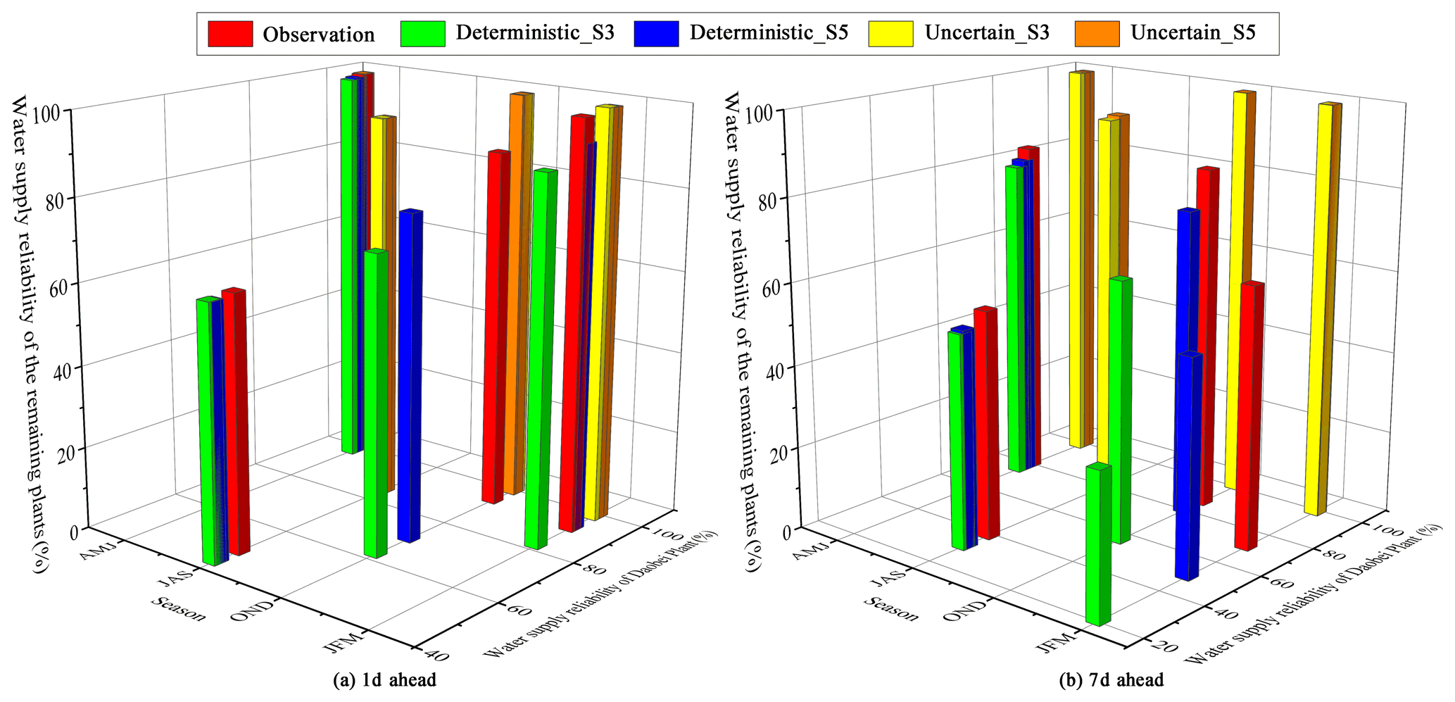
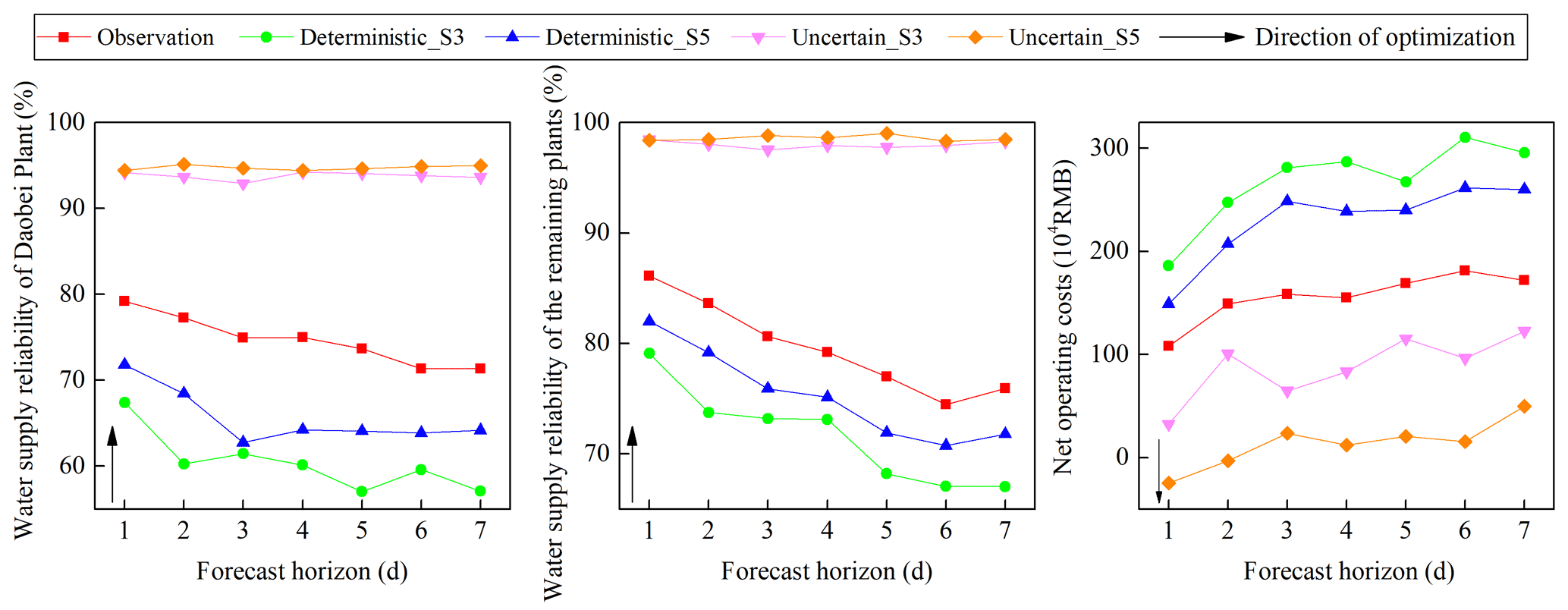
Table 6Annual system performance using forecast inflow information.
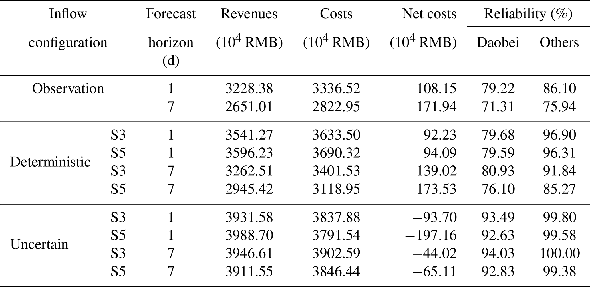
Table 7Annual system performance using observed inflow information.
Our work suffers from some limitations which could be overcome in future studies. One of the limitations is that only one single indicator was used to calibrate the forecast models, while multiple indicators were used in assessing the performance of the models. It would be a more fair practice to use multi-criteria to do both calibration and assessment, and this could be interesting for future work. Another limitation is that we used the average observed price to calculate the revenues and operating costs. In an operational and deregulated market setting, the prices may fluctuate significantly (Anghileri et al., 2019). For instance, forecasting electricity prices is likely to improve short-term operation efficiency significantly. The combined effects of price and streamflow forecasts on water resource allocation are worth investigating in future studies. Our study also suffers from the drawback that instead of using the short-term weather forecasts from the Global Forecast System (GFS) or European Centre for Medium-Range Weather Forecasts (ECMWF) model (Choong and El-Shafie, 2015; Schwanenberg et al., 2015; Peng et al., 2018; Ahmad and Hossain, 2019; Liu et al., 2019), we used the observed weather conditions as alternatives, which may result in an overestimation in forecast quality. However, forecast uncertainty and error generally grow with lead time. The usefulness of the forecast information is reduced with the increase of the forecast horizon and thus the operating performance. This may influence the finding we highlight above that the relationship between the forecast horizon and reservoir operation is not constant and specific. It would be interesting to analyze the reservoir operation performance when accounting for an ensemble numerical weather prediction.
In this study, we proposed an AI-based management methodology to assess forecast quality and forecast-informed reservoir operation performance together. The approach was tested on a water resources allocation system in Zhoushan Islands, China. Specifically, the findings are summarized below.
A data-driven reservoir inflow forecasting system using ML methods (LSTM, GRU, and GWO-LSSVM) was first developed with a comprehensive calibration–validation–testing framework. The validity of the deterministic forecast was demonstrated by applying it over 25 reservoirs with varying climate and hydrological characteristics. Results showed that the more variation the streamflow has (a high COV value), the harder it was for the ML methods to learn the flow pattern when there was not enough input information. The forecast skill deteriorated with increasing lead times under such scenarios. However, short-term forecast climate forcing was efficient and scalable in forecasting the multi-reservoir inflow over the forecast horizon (1–7 d). LSTM and GRU models generated comparable performance under different configurations. Given that GRU has simpler structures and fewer parameters and required less time for modeling, it might be the preferred method for streamflow forecasts than LSTM.
Then we used BMA to generate stochastic inflow scenarios for quantifying uncertainty based on LSTM, GRU, and GWO-LSSVM deterministic forecasts. The results demonstrated that it was difficult to conclude which individual model provided the best prediction, but the BMA did display better forecast skills in comparison to the individual ones. Including one scenario with antecedent conditions and one scenario with both antecedent and forecast information, two input combination scenarios were compared on the uncertain forecast performance in detail. The comparison indicated that forecast climate variables would help reduce the predictive uncertainty of short-term streamflow forecasting.
The forecasting scheme was further coupled with a multi-objective reservoir operation model to optimize water resources allocation. Using a MORDM approach, we identified strategies that were useful for a tradeoff between water supply reliability and operating costs in Zhoushan Islands. A rolling horizon scheme was employed to obtain an optimal operating policy over the horizon of 1–7 d. The long-term assessment over a year based on deterministic and stochastic forecasts showed quite different performances in terms of water supply reliability and net operating costs. Our averaged annual results showed that uncertain forecasts were more valuable than deterministic forecasts. The operating benefits of considering the forecasts were more significant when the forecast quality was higher. Similar results could be obtained at a seasonal scale. While showing the unquestionable benefit of implementing forecast-based reservoir operations, our results also demonstrated that the relationship between the forecast horizon and reservoir operation was complex and depended on the operating configurations (forecast quality and uncertainty) and performance measures for the Zhoushan Islands system.
Overall, the developed AI-based management framework has demonstrated a clear advantage in quantifying the uncertainties of inflow forecasts to improve the overall system performance of water allocation systems. Such a framework can be further applied to other study sites with similar problems. However, the results we obtained in this study are only specific to the Zhoushan Islands and should be applied to other study sites with care.
The data used to support the findings of this study are available from the corresponding author upon request.
YG and YPX designed all the experiments. HC and HG collected and preprocessed the data. YG and XY conducted all the experiments and analyzed the results. YG wrote the first draft of the manuscript with contributions from JX. YPX supervised the study and edited the manuscript.
The authors declare that they have no conflict of interest.
Publisher's note: Copernicus Publications remains neutral with regard to jurisdictional claims in published maps and institutional affiliations.
The editors and two reviewers are greatly acknowledged for their constructive comments to improve the quality of this paper.
This research has been supported by the Key Project of Zhejiang Natural Science Foundation (grant no. LZ20E090001), the Zhejiang Key Research and Development Program (2021C03017), and the Fundamental Research Funds for the Zhejiang Provincial Universities (2021XZZX015).
This paper was edited by Dimitri Solomatine and reviewed by two anonymous referees.
Adnan, R. M., Liang, Z., Heddam, S., Zounemat-Kermani, M., Kisi, O., and Li, B.: Least square support vector machine and multivariate adaptive regression splines for streamflow prediction in mountainous basin using hydro-meteorological data as inputs, J. Hydrol., 586, 124371, https://doi.org/10.1016/j.jhydrol.2019.124371, 2020.
Ahmad, S. K. and Hossain, F.: A generic data-driven technique for forecasting of reservoir inflow: Application for hydropower maximization, Environ. Model. Softw., 119, 147–165, https://doi.org/10.1016/j.envsoft.2019.06.008, 2019.
Alexander, S., Yang, G., Addisu, G., and Block, P.: Forecast-informed reservoir operations to guide hydropower and agriculture allocations in the Blue Nile basin, Ethiopia, Int. J. Water Resour. Dev., 37, 208–233, https://doi.org/10.1080/07900627.2020.1745159, 2020.
Ali, S. and Shahbaz, M.: Streamflow forecasting by modeling the rainfall–streamflow relationship using artificial neural networks, Model. Earth Syst. Environ., 6, 1645–1656, https://doi.org/10.1007/s40808-020-00780-3, 2020.
Al-Sudani, Z. A., Salih, S. Q., and Yaseen, Z. M.: Development of multivariate adaptive regression spline integrated with differential evolution model for streamflow simulation, J. Hydrol., 573, 1–12, https://doi.org/10.1016/j.jhydrol.2019.03.004, 2019.
Anghileri, D., Monhart, S., Zhou, C., Bogner, K., Castelletti, A., Burlando, P., and Zappa, M.: Value of long-term streamflow forecasts to reservoir operations for water supply in snow-dominated river catchments, Water Resour. Res., 52, 4209–4225, https://doi.org/10.1002/2015WR017864, 2016.
Anghileri, D., Voisin, N., Castelletti, A., Pianosi, F., Nijssen, B., and Lettenmaier, D. P.: The Value of Subseasonal Hydrometeorological Forecasts to Hydropower Operations: How Much Does Preprocessing Matter?, Water Resour. Res., 55, 10159–10178, https://doi.org/10.1029/2019WR025280, 2019.
Ayzel, G. and Heistermann, M.: The effect of calibration data length on the performance of a conceptual hydrological model versus LSTM and GRU: A case study for six basins from the CAMELS dataset, Comput. Geosci., 149, 104708, https://doi.org/10.1016/j.cageo.2021.104708, 2021.
Bemani, A., Xiong, Q., Baghban, A., Habibzadeh, S., Mohammadi, A. H., and Doranehgard, M. H.: Modeling of cetane number of biodiesel from fatty acid methyl ester (FAME) information using GA-, PSO-, and HGAPSO-LSSVM models, Renew. Energy, 150, 924–934, https://doi.org/10.1016/j.renene.2019.12.086, 2020.
Ben Taieb, S., Bontempi, G., Atiya, A. F., and Sorjamaa, A.: A review and comparison of strategies for multi-step ahead time series forecasting based on the NN5 forecasting competition, Exp. Syst. Appl., 39, 7067–7083, https://doi.org/10.1016/j.eswa.2012.01.039, 2012.
Boucher, M. A., Tremblay, D., Delorme, L., Perreault, L., and Anctil, F.: Hydro-economic assessment of hydrological forecasting systems, J. Hydrol., 416, 133–144, https://doi.org/10.1016/j.jhydrol.2011.11.042, 2012.
Cheng, M., Fang, F., Kinouchi, T., Navon, I. M., and Pain, C. C.: Long lead-time daily and monthly streamflow forecasting using machine learning methods, J. Hydrol., 590, 125376, https://doi.org/10.1016/j.jhydrol.2020.125376, 2020.
Chiew, F., Zhou, S., and McMahon, T.: Use of seasonal streamflow forecasts in water resources management, J. Hydrol., 270, 135–144, https://doi.org/10.1016/S0022-1694(02)00292-5, 2003.
Cho, K., Merrienboer, B. v., Gulcehre, C., Bahdanau, D., Bougares, F., Schwenk, H., and Bengio, Y.: Learning Phrase Representations using RNN Encoder-Decoder for Statistical Machine Translation, Comput. Sci., arxiv: perprint: http://arxiv.org/abs/1406.1078v3 (last access: 14 November 2021), 2014.
Choong, S.-M. and El-Shafie, A.: State-of-the-Art for Modelling Reservoir Inflows and Management Optimization, Water Resour. Manage., 29, 1267–1282, https://doi.org/10.1007/s11269-014-0872-z, 2015.
Deisenroth, M., Neumann, G., and Peters, J.: A Survey on Policy Search for Robotics, Foundat. Trends Robot., 2, 1–142, https://doi.org/10.1561/2300000021, 2013.
Denaro, S., Anghileri, D., Giuliani, M., and Castelletti, A.: Informing the operations of water reservoirs over multiple temporal scales by direct use of hydro-meteorological data, Adv. Water Resour., 103, 51–63, https://doi.org/10.1016/j.advwatres.2017.02.012, 2017.
Elman, J. L.: Finding Structure in Time, Cognit. Sci., 14, 179–211, https://doi.org/10.1207/s15516709cog1402_1, 1990.
Fang, G., Guo, Y., Huang, X., Rutten, M., and Yuan, Y.: Combining Grey Relational Analysis and a Bayesian Model Averaging Method to Derive Monthly Optimal Operating Rules for a Hydropower Reservoir. Water, 10, 1099, https://doi.org/10.3390/w10081099, 2018a.
Fang, G., Guo, Y., Wen, X., Fu, X., Lei, X., and Tian, Y.: Multi-Objective Differential Evolution-Chaos Shuffled Frog Leaping Algorithm for Water Resources System Optimization, Water Resour. Manage., 32, 3835–3852, https://doi.org/10.1007/s11269-018-2021-6, 2018b.
Feng, D., Fang, K., and Shen, C.: Enhancing streamflow forecast and extracting insights using long-short term memory networks with data integration at continental scales, Water Resour. Res., 56, e2019WR026793, https://doi.org/10.1029/2019WR026793, 2020.
Gao, S., Huang, Y., Zhang, S., Han, J., Wang, G., Zhang, M., and Lin, Q.: Short-term runoff prediction with GRU and LSTM networks without requiring time step optimization during sample generation, J. Hydrol., 589, 125188, https://doi.org/10.1016/j.jhydrol.2020.125188, 2020.
Ghumman, A. R., Ahmad, S., and Hashmi, H. N.: Performance assessment of artificial neural networks and support vector regression models for stream flow predictions, Environ. Monit. Assess., 190, 704, https://doi.org/10.1007/s10661-018-7012-9, 2018.
Gibbs, M. S., McInerney, D., Humphrey, G., Thyer, M. A., Maier, H. R., Dandy, G. C., and Kavetski, D.: State updating and calibration period selection to improve dynamic monthly streamflow forecasts for an environmental flow management application, Hydrol. Earth Syst. Sci., 22, 871–887, https://doi.org/10.5194/hess-22-871-2018, 2018.
Giuliani, M. and Castelletti, A.: Is robustness really robust? How different definitions of robustness impact decision-making under climate change, Climatic Change, 135, 409–424, https://doi.org/10.1007/s10584-015-1586-9, 2016.
Giuliani, M., Herman, J., Castelletti, A., and Reed, P.: Many-objective reservoir policy identification and refinement to reduce policy inertia and myopia in water management, Water Resour. Res., 50, 3355–3377, https://doi.org/10.1002/2013WR014700, 2014.
Giuliani, M., Pianosi, F., and Castelletti, A.: Making the most of data: an information selection and assessment framework to improve water systemsoperations, Water Resour. Res., 51, 9073–9093, https://doi.org/10.1002/2015WR017044, 2015.
Giuliani, M., Castelletti, A., Pianosi, F., Mason, E., and Reed, P. M.: Curses, tradeoffs, and scalable management: Advancing evolutionary multiobjective direct policy search to improve water reservoir operations, J. Water Resour. Pl. Manage., 142, 04015050, https://doi.org/10.5334/jors.293, 2016.
Goddard, L., Aitchellouche, Y., Baethgen, W., Dettinger, M., Graham, R., Hayman, P., Kadi, M., Martínez, R., and Meinke, H.: Providing Seasonal-to-Interannual Climate Information for Risk Management and Decision-making, Proced. Environ. Sci., 1, 81–101, https://doi.org/10.1016/j.proenv.2010.09.007, 2010.
Greff, K., Srivastava, R. K., Koutník, J., Steunebrink, B. R., and Schmidhuber, J.: LSTM: A Search Space Odyssey, IEEE T. Neural Netw. Learn. Syst., 28, 2222–2232, https://doi.org/10.1109/TNNLS.2016.2582924, 2017.
Guo, Y., Fang, G., Wen, X., Lei, X., Yuan, Y., and Fu, X.: Hydrological responses and adaptive potential of cascaded reservoirs under climate change in Yuan River Basin, Hydrol. Res., 50, 358–378, https://doi.org/10.2166/nh.2018.165, 2018.
Guo, Y., Fang, G., Xu, Y.-P., Tian, X., and Xie, J.: Identifying how future climate and land use/cover changes impact streamflow in Xinanjiang Basin, East China, Sci. Total Environ., 710, 136275, https://doi.org/10.1016/j.scitotenv.2019.136275, 2020a.
Guo, Y., Fang, G., Xu, Y.-P., Tian, X., and Xie, J.: Responses of hydropower generation and sustainability to changes in reservoir policy, climate and land use under uncertainty: A case study of Xinanjiang Reservoir in China, J. Clean. Product., 281, 124609, https://doi.org/10.1016/j.jclepro.2020.124609, 2020b.
Guo, Y., Tian, X., Fang, G., and Xu, Y.-P.: Many-objective optimization with improved shuffled frog leaping algorithm for inter-basin water transfers, Adv. Water Resour., 138, 103531, https://doi.org/10.1016/j.advwatres.2020.103531, 2020c.
Guo, Y., Xu, Y.-P., Sun, M., and Xie, J.: Multi-step-ahead forecast of reservoir water availability with improved quantum-based GWO coupled with the AI-based LSSVM model, J. Hydrol., 597, 125769, https://doi.org/10.1016/j.jhydrol.2020.125769, 2020d.
Hadi, S. J., Tombul, M., Salih, S. Q., Al-Ansari, N., and Yaseen, Z. M.: The capacity of the hybridizing wavelet transformation approach with data-driven models for modeling monthly-scale streamflow, IEEE Access, 8, 101993–102006, https://doi.org/10.1109/ACCESS.2020.2998437, 2020.
Hadjimichael, A., Gold, D., Hadka, D., and Reed, P.: Rhodium: Python Library for Many-Objective Robust Decision Making and Exploratory Modeling, J. Open Res. Softw., 8, 12, https://doi.org/10.5334/jors.293, 2020.
Hochreiter, S. and Schmidhuber, J.: Long Short-Term Memory, Neural Comput., 9, 1735–1780, https://doi.org/10.1162/neco.1997.9.8.1735, 1997.
Hoeting, J. A., Madigan, D., Raftery, A. E., and Volinsky, C. T.: Bayesian Model Averaging: A Tutorial, Stat. Sci., 14, 382–417, 1999.
Jung, Y., Jung, J., Kim, B., and Han, S.: Long short-term memory recurrent neural network for modeling temporal patterns in long-term power forecasting for solar PV facilities: Case study of South Korea, J. Clean. Product., 250, 119476, https://doi.org/10.1016/j.jclepro.2019.119476, 2020.
Karunanithi, N., Grenney, W. J., Whitley, D., and Bovee, K.: Neural networks for river flow prediction, J. Comput. Civ. Eng., 8, 201–220, https://doi.org/10.1061/(ASCE)0887-3801(1994)8:2(201), 1994.
Kasprzyk, J. R., Nataraj, S., Reed, P. M., and Lempert, R.: Many objective robust decision making for complex environmental systems undergoing change, Environ. Model. Softw., 42, 55–71, https://doi.org/10.1016/j.envsoft.2012.12.007, 2013.
Kisi, O., Choubin, B., Deo, R. C., and Yaseen, Z. M.: Incorporating synoptic-scale climate signals for streamflow modelling over the Mediterranean region using machine learning models, Hydrolog. Sci. J., 64, 1240–1252, https://doi.org/10.1080/02626667.2019.1632460, 2019.
Kline, D.: Methods for Multi-Step Time Series Forecasting with Neural Networks, Neural Networks in Business Forecasting, IGI Global, USA, 226–250, https://doi.org/10.4018/978-1-59140-176-6.ch012, 2004.
Lee, S., Yen, H., Yeo, I.-Y., Moglen, G. E., Rabenhorst, M. C., and McCarty, G. W.: Use of multiple modules and Bayesian Model Averaging to assess structural uncertainty of catchment-scale wetland modeling in a Coastal Plain landscape, J. Hydrol., 582, 124544, https://doi.org/10.1016/j.jhydrol.2020.124544, 2020.
Legates, D. R. and McCabe Jr., G. J.: Evaluating the use of “goodness-of-fit” Measures in hydrologic and hydroclimatic model validation, Water Resour. Res., 35, 233–241, https://doi.org/10.1029/1998WR900018, 1999.
Liu, L., Xu, Y. P., Pan, S. L., and Bai, Z. X.: Potential application of hydrological ensemble prediction in forecasting floods and its components over the Yarlung Zangbo River basin, China, Hydrol. Earth Syst. Sci., 23, 3335–3352, https://doi.org/10.5194/hess-23-3335-2019, 2019.
Liu, Z. and Merwade, V.: Separation and prioritization of uncertainty sources in a raster based flood inundation model using hierarchical Bayesian model averaging, J. Hydrol., 578, 124100, https://doi.org/10.1016/j.jhydrol.2019.124100, 2019.
Maurer, E. P. and Lettenmaier, D. P.: Potential effects of long-lead hydrologic predictability on Missouri River main-stem reservoirs, J. Climate, 17, 174–186, https://doi.org/10.1175/1520-0442(2004)017<0174:PEOLHP>2.0.CO;2, 2004.
Mehdizadeh, S., Fathian, F., Safari, M. J. S., and Adamowski, J. F.: Comparative assessment of time series and artificial intelligence models to estimate monthly streamflow: A local and external data analysis approach, J. Hydrol., 579, 124225, https://doi.org/10.1016/j.jhydrol.2019.124225, 2019.
Meng, E., Huang, S., Huang, Q., Fang, W., Wu, L., and Wang, L.: A robust method for non-stationary streamflow prediction based on improved EMD-SVM model, J. Hydrol., 568, 462–478, https://doi.org/10.1016/j.jhydrol.2018.11.015, 2019.
Muhammad, A. U., Li, X., and Feng, J.: Using LSTM GRU and Hybrid Models for Streamflow Forecasting, in: Machine Learning and Intelligent Communications 2019, Lecture Notes of the Institute for Computer Sciences, Social Informatics and Telecommunications Engineering, Springer, 294, 510–524, https://doi.org/10.1007/978-3-030-32388-2_44, 2019.
Nanda, T., Sahoo, B., and Chatterjee, C.: Enhancing real-time streamflow forecasts with wavelet-neural network based error-updating schemes and ECMWF meteorological predictions in Variable Infiltration Capacity model, J. Hydrol., 575, 890–910, https://doi.org/10.1016/j.jhydrol.2019.05.051, 2019.
Nash, J. E. and Sutcliffe, J. V.: River flow forecasting through conceptual models part I – A discussion of principles, J. Hydrol., 10, 282–290, https://doi.org/10.1016/0022-1694(70)90255-6, 1970.
Nott, D. J., Marshall, L., and Brown, J.: Generalized likelihood uncertainty estimation (GLUE) and approximate Bayesian computation: What's the connection?, Water Resour. Res., 48, W12602, https://doi.org/10.1029/2011WR011128, 2012.
Osman, A., Afan, H. A., Allawi, M. F., Jaafar, O., Noureldin, A., Hamzah, F. M., Ahmed, A. N., and El-shafie, A.: Adaptive Fast Orthogonal Search (FOS) algorithm for forecasting streamflow, J. Hydrol., 586, 124896, https://doi.org/10.1016/j.jhydrol.2020.124896, 2020.
Pechlivanidis, I., Crochemore, L., Rosberg, J., and Bosshard, T.: What are the key drivers controlling the quality of seasonal streamflow forecasts?, Water Resour. Res., 56, e2019WR026987, https://doi.org/10.1029/2019WR026987, 2020.
Peng, A., Zhang, X., Peng, Y., Xu, W., and You, F.: The application of ensemble precipitation forecasts to reservoir operation, Water Supply, 19, 588–595, https://doi.org/10.2166/ws.2018.105, 2018.
Pishvaee, M. S. and Razmi, J.: Environmental supply chain network design using multi-objective fuzzy mathematical programming, Appl. Math. Model., 36, 3433–3446, https://doi.org/10.1016/j.apm.2011.10.007, 2012.
Quinn, J. D., Reed, P. M., Giuliani, M., and Castelletti, A.: Rival framings: A framework for discovering how problem formulation uncertainties shape risk management trade-offs in water resources systems, Water Resour. Res., 53, 7208–7233, https://doi.org/10.1002/2017WR020524, 2017a.
Quinn, J. D., Reed, P. M., and Keller, K.: Direct policy search for robust multi-objective management of deeply uncertain socio-ecological tipping points, Environ. Model. Softw., 92, 125–141, https://doi.org/10.1016/j.envsoft.2017.02.017, 2017b.
Ren, C., Guo, P., Tan, Q., and Zhang, L.: A multi-objective fuzzy programming model for optimal use of irrigation water and land resources under uncertainty in Gansu Province, China, J. Clean. Product., 164, 85–94, https://doi.org/10.1016/j.jclepro.2017.06.185, 2017.
Roulston, M. S. and Smith, L. A.: Combining dynamical and statistical ensembles, Tellus A, 55, 16–30, https://doi.org/10.3402/tellusa.v55i1.12082, 2003.
Salazar, J. Z., Reed, P. M., Quinn, J. D., Giuliani, M., and Castelletti, A.: Balancing exploration, uncertainty and computational demands in many objective reservoir optimization, Adv. Water Resour., 109, 196–210, https://doi.org/10.1016/j.advwatres.2017.09.014, 2017.
Samadi, S., Pourreza-Bilondi, M., Wilson, C., and Hitchcock, D.: Bayesian model averaging with fixed and flexible priors: Theory, concepts, and calibration experiments for rainfall-runoff modeling, J. Adv. Model. Earth Syst., 12, e2019MS001924, https://doi.org/10.1029/2019MS001924, 2020.
Schwanenberg, D., Fan, F. M., Naumann, S., Kuwajima, J. I., Montero, R. A., and Assis dos Reis, A.: Short-Term Reservoir Optimization for Flood Mitigation under Meteorological and Hydrological Forecast Uncertainty, Water Resour. Manage., 29, 1635–1651, https://doi.org/10.1007/s11269-014-0899-1, 2015.
Shahid, F., Zameer, A., and Muneeb, M.: Predictions for COVID-19 with deep learning models of LSTM, GRU and Bi-LSTM, Chaos Solit. Fract., 140, 110212, https://doi.org/10.1016/j.chaos.2020.110212, 2020.
Shamir, E.: The value and skill of seasonal forecasts for water resources management in the Upper Santa Cruz River basin, southern Arizona, J. Arid Environ., 137, 35–45, https://doi.org/10.1016/j.jaridenv.2016.10.011, 2017.
Sharma, S., Siddique, R., Reed, S., Ahnert, P., and Mejia, A.: Hydrological Model Diversity Enhances Streamflow Forecast Skill at Short-to Medium-Range Timescales, Water Resour. Res., 55, 1510–1530, https://doi.org/10.1029/2018WR023197, 2019.
Suykens, J. A. K. and Vandewalle, J.: Least Squares Support Vector Machine Classifiers, Neural Process. Lett., 9, 293–300, https://doi.org/10.1023/A:1018628609742, 1999.
Suykens, J. A. K., Van Gestel, T., De Brabanter, J., De Moor, B., and Vandewalle, J.: Least Squares Support Vector Machines, World Scientific Publishing, Singapore, 2002.
Tikhamarine, Y., Souag-Gamane, D., Najah Ahmed, A., Kisi, O., and El-Shafie, A.: Improving artificial intelligence models accuracy for monthly streamflow forecasting using grey Wolf optimization (GWO) algorithm, J. Hydrol., 582, 124435, https://doi.org/10.1016/j.jhydrol.2019.124435, 2020.
Turner, S., Bennett, J., Robertson, D., and Galelli, S.: Complex relationship between seasonal streamflow forecast skill and value in reservoir operations, Hydrol. Earth Syst. Sci., 21, 4841–4859, https://doi.org/10.5194/hess-21-4841-2017, 2017.
Van Osnabrugge, B., Uijlenhoet, R., and Weerts, A.: Contribution of potential evaporation forecasts to 10-day streamflow forecast skill for the Rhine River, Hydrol. Earth Syst. Sci., 23, 1453–1467, https://doi.org/10.5194/hess-23-1453-2019, 2019.
Xiong, L., Wan, M., Wei, X., and O'connor, K. M.: Indices for assessing the prediction bounds of hydrological models and application by generalised likelihood uncertainty estimation, Hydrolog. Sci. J., 54, 852–871, https://doi.org/10.1623/hysj.54.5.852, 2009.
Xu, B., Zhong, P.-a., Lu, Q., Zhu, F., Huang, X., Ma, Y., and Fu, J.: Multiobjective stochastic programming with recourses for real-time flood water conservation of a multireservoir system under uncertain forecasts, J. Hydrol., 590, 125513, https://doi.org/10.1016/j.jhydrol.2020.125513, 2020.
Xu, W., Zhang, C., Peng, Y., Fu, G., and Zhou, H.: A two stage B ayesian stochastic optimization model for cascaded hydropower systems considering varying uncertainty of flow forecasts, Water Resour. Res., 50, 9267–9286, https://doi.org/10.1002/2013WR015181, 2014.
Yan, D., Ludwig, F., Huang, H. Q., and Werners, S. E.: Many-objective robust decision making for water allocation under climate change, Sci. Total Environ., 607, 294–303, https://doi.org/10.1016/j.scitotenv.2017.06.265, 2017.
Yang, G., Guo, S., Liu, P., Li, L., and Xu, C.: Multiobjective reservoir operating rules based on cascade reservoir input variable selection method, Water Resour. Res., 53, 3446–3463, https://doi.org/10.1002/2016WR020301, 2017.
Zeff, H. B., Kasprzyk, J. R., Herman, J. D., Reed, P. M., and Characklis, G. W.: Navigating financial and supply reliability tradeoffs in regional drought management portfolios, Water Resour. Res., 50, 4906–4923, https://doi.org/10.1002/2013WR015126, 2014.
Zhai, B. and Chen, J.: Development of a stacked ensemble model for forecasting and analyzing daily average PM2.5 concentrations in Beijing, China, Sci. Total Environ., 635, 644–658, https://doi.org/10.1016/j.scitotenv.2018.04.040, 2018.
Zhang, D., Lindholm, G., and Ratnaweera, H.: Use long short-term memory to enhance Internet of Things for combined sewer overflow monitoring, J. Hydrol., 556, 409–418, https://doi.org/10.1016/j.jhydrol.2017.11.018, 2018.
Zhang, F., Guo, S., Liu, X., Wang, Y., Engel, B. A., and Guo, P.: Towards sustainable water management in an arid agricultural region: A multi-level multi-objective stochastic approach, Agricult. Syst., 182, 102848, https://doi.org/10.1016/j.agsy.2020.102848, 2020.
Zhang, J., Liu, P., Wang, H., Lei, X., and Zhou, Y.: A Bayesian model averaging method for the derivation of reservoir operating rules, J. Hydrol., 528, 276–285, https://doi.org/10.1016/j.jhydrol.2015.06.041, 2015.
Zhao, Q., Cai, X., and Li, Y.: Determining Inflow Forecast Horizon for Reservoir Operation, Water Resour. Res., 55, 4066–4081, https://doi.org/10.1029/2019WR025226, 2019.
Zhou, Y., Chang, F.-J., Chen, H., and Li, H.: Exploring Copula-based Bayesian Model Averaging with multiple ANNs for PM2.5 ensemble forecasts, J. Clean. Product., 263, 121528, https://doi.org/10.1016/j.jclepro.2020.121528, 2020a.
Zhou, Y., Chang, L.-C., and Chang, F.-J.: Explore a Multivariate Bayesian Uncertainty Processor driven by artificial neural networks for probabilistic PM2.5 forecasting, Sci. Total Environ., 711, 134792, https://doi.org/10.1016/j.scitotenv.2019.134792, 2020b.
Zimmermann, H.-J.: Fuzzy programming and linear programming with several objective functions, Fuzzy Sets Syst., 1, 45–55, https://doi.org/10.1016/0165-0114(78)90031-3, 1978.
Zuo, G., Luo, J., Wang, N., Lian, Y., and He, X.: Decomposition ensemble model based on variational mode decomposition and long short-term memory for streamflow forecasting, J. Hydrol., 585, 124776, https://doi.org/10.1016/j.jhydrol.2020.124776, 2020.