the Creative Commons Attribution 4.0 License.
the Creative Commons Attribution 4.0 License.
 | 11 Nov 2021
Large-scale sensitivities of groundwater and surface water to groundwater withdrawal
Edwin H. Sutanudjaja
Niko Wanders
Increasing population, economic growth and changes in diet have dramatically increased the demand for food and water over the last decades. To meet increasing demands, irrigated agriculture has expanded into semi-arid areas with limited precipitation and surface water availability. This has greatly intensified the dependence of irrigated crops on groundwater withdrawal and caused a steady increase in groundwater withdrawal and groundwater depletion. One of the effects of groundwater pumping is the reduction in streamflow through capture of groundwater recharge, with detrimental effects on aquatic ecosystems. The degree to which groundwater withdrawal affects streamflow or groundwater storage depends on the nature of the groundwater–surface water interaction (GWSI). So far, analytical solutions that have been derived to calculate the impact of groundwater on streamflow depletion involve single wells and streams and do not allow the GWSI to shift from connected to disconnected, i.e. from a situation with two-way interaction to one with a one-way interaction between groundwater and surface water. Including this shift and also analysing the effects of many wells requires numerical groundwater models that are expensive to set up. Here, we introduce an analytical framework based on a simple lumped conceptual model that allows us to estimate to what extent groundwater withdrawal affects groundwater heads and streamflow at regional scales. It accounts for a shift in GWSI, calculates at which critical withdrawal rate such a shift is expected, and when it is likely to occur after withdrawal commences. It also provides estimates of streamflow depletion and which part of the groundwater withdrawal comes out of groundwater storage and which parts from a reduction in streamflow. After a local sensitivity analysis, the framework is combined with parameters and inputs from a global hydrological model and subsequently used to provide global maps of critical withdrawal rates and timing, the areas where current withdrawal exceeds critical limits and maps of groundwater and streamflow depletion rates that result from groundwater withdrawal. The resulting global depletion rates are compared with estimates from in situ observations and regional and global groundwater models and satellites. Pairing of the analytical framework with more complex global hydrological models presents a screening tool for fast first-order assessments of regional-scale groundwater sustainability and for supporting hydro-economic models that require simple relationships between groundwater withdrawal rates and the evolution of pumping costs and environmental externalities.
- Article
(5312 KB) - Full-text XML
-
Supplement
(1725 KB) - BibTeX
- EndNote


Increasing population, economic growth and changes in diet have dramatically increased the demand for food and water over the last decades (Godfray et al., 2010). To meet increasing demands, irrigated agriculture has expanded into semi-arid areas with limited precipitation and surface water (Siebert et al., 2015). This has greatly intensified the dependence of irrigated crops on groundwater withdrawal (Wada et al., 2012) and caused a steady increase in groundwater depletion rates (Wada and Bierkens, 2019). Recent estimates of the current groundwater withdrawal range approximately between 600 and 1000 km3 yr−1, leading to estimated depletion rates of 150–400 km3 yr−1 (Wada, 2016).
Groundwater that is pumped comes either out of storage, from reduced groundwater discharge, or from reduction of evaporation fed from below by groundwater through capillary rise and/or phreatophytes (Theis, 1940; Alley et al., 1999; Bredehoeft, 2002; Konikow and Leake, 2014). Thus, extensive groundwater pumping not only leads to groundwater depletion (Wada et al., 2010), but also to a reduction in streamflow (Wada et al., 2013; Mukherjee et al., 2019; De Graaf et al., 2019; Jasechko et al., 2021) and desiccation of wetlands and groundwater-dependent terrestrial ecosystems (Runhaar et al., 1997; Shafroth et al., 2000; Elmore et al., 2006; Yin et al., 2018). However, the effect of groundwater pumping on groundwater depletion and surface water depletion heavily depends on the nature of the interaction between groundwater and surface water. Limiting ourselves to phreatic groundwater systems, and following Winter et al. (1998), a distinction can be made between gaining streams, loosing streams, and disconnected loosing streams, depending on the position of the free groundwater surface with respect to the surface water level and the bottom of the stream (Fig. 1). Since groundwater pumping affects groundwater levels, it can move a stream from gaining to loosing to disconnected and loosing, which, in turn, affects the way that groundwater pumping affects streamflow.
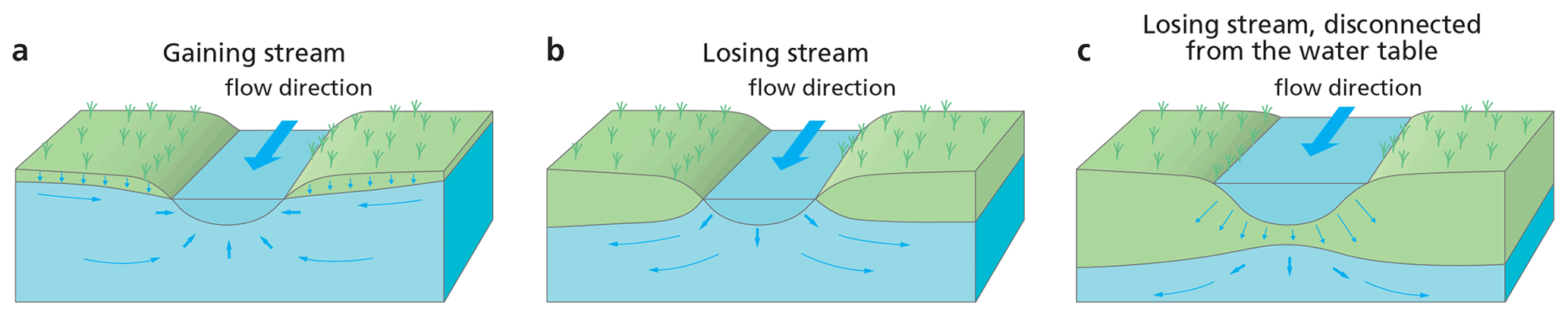
Figure 1Groundwater–streamflow interaction: (a) gaining stream; (b) losing stream; (c) losing stream disconnected from the water table, modified from Winter at al. (1998). Credit to the United States Geological Survey.
Based on the above, Bierkens and Wada (2019) define two stages of groundwater withdrawal in phreatic aquifers. In stage 1, groundwater withdrawal is such that the water table remains connected to the surface water system (Fig. 1a, b). Upon pumping, groundwater initially comes out of storage, and groundwater levels decline. However, as groundwater levels decline around a well, the well attracts more of the recharge that would otherwise end up in the stream until a new equilibrium is reached, where all of the pumped water comes out of captured streamflow. In a stage 1 withdrawal regime, withdrawal can be considered physically stable, where groundwater depletion is limited and groundwater withdrawal mostly diminishes streamflow and evaporation. Depending on the groundwater level, one could further distinguish between gaining (Fig. 1a) and loosing (Fig. 1b) streams. This is important when considering the quality of pumped groundwater, as in the case of loosing stream surface water may end up in the well. In a stage 2 withdrawal regime, groundwater withdrawal is so large that groundwater levels fall below the bottom of the stream (Fig. 1c). In that case, a further decline in the groundwater level hardly increases infiltration from the stream to the aquifer. Thus, in stage 2, groundwater withdrawal in excess of recharge and (constant) stream water infiltration is physically unstable and as a result leads to groundwater depletion and does not impact streamflow further if pumping rates increase.
From the above it follows that there is a critical transition between stage 1 and stage 2 groundwater withdrawal that depends on the groundwater withdrawal rate. In reality, this transition is less abrupt. Right after the water table is just below the river bottom, negative pressure heads occur below the river bed while the soil is fully or partly saturated. Wang et al. (2015) show experimentally and theoretically that a full disconnection, i.e. the water table has no impact on the infiltration flux, occurs only when the depth of the groundwater table below the stream becomes larger than the stream water depth. Another reason that this transition does not occur abruptly is that multiple surface water bodies in the surroundings of groundwater wells differ in depth depending on stream order and location in the river basin. We also note that in many regions of the world groundwater is pumped from deeper-confined or leaky-confined aquifers (De Graaf et al., 2017). Under confined conditions, groundwater–streamflow interaction only occurs for the larger rivers that are deep enough to penetrate the confining layer, while in leaky-confined aquifers the interactions are more complicated and delayed (Hunt, 2003).
There are many analytical solutions for calculating the stream depletion rate (SDR), defined as the ratio of the volumetric rate of water abstraction from a stream water to groundwater pumping rate. These solutions differ in assumptions about the type of aquifer (unconfined, confined, leaky-confined, multiple aquifers), stream bottom elevation, and stream geometry and including additional resistance from the streambed clogging layer or not. We refer to Huang et al. (2018) for an extensive overview of solutions and when to apply them. These analytical solutions typically involve a single well and a single stream, or, using apportionment methods, a single well and stream networks (Zipper et al., 2019), while they consider streams to be connected to the water table. Such analytical solutions could possibly be used for multiple wells using e.g. superposition. However, for more complex situations, with multiple wells, increasing withdrawal rates and streams changing from e.g. connected to disconnected, numerical groundwater models need to be used. These have the disadvantage that they are parameter-greedy, are time-consuming to set up, and are often computationally expensive. Thus, relatively simple analytical tools to assess the effects of extensive multi-well groundwater pumping on groundwater and surface water systems at large scale are lacking.
Here, we introduce a simple analytical framework based on a lumped conceptual model of aquifer–stream interaction under pumping. The framework aims to describe at larger scales, i.e. large catchments and/or regional-scale phreatic aquifer systems, to what extent multi-well groundwater withdrawal affects area-average groundwater heads and streamflow. It allows for a shift in the nature of groundwater–surface water interaction and calculates at which critical withdrawal rate such a shift is expected and when it is likely to occur after withdrawal commences. It also provides estimates of streamflow depletion and the partitioning between groundwater storage depletion and reduction in streamflow (capture). We envision that such an analytical framework, when parameterized with parameters and inputs from a more complex global-scale hydrological model, can be used as a screening tool for fast first-order assessments of regional-scale groundwater sustainability and for supporting hydro-economic models that require simple relationships between large-scale groundwater withdrawal rates and the evolution of pumping costs and environmental externalities.
In the following, we first introduce the lumped conceptual model of large-scale groundwater pumping with groundwater–surface water interaction. Next, we show its properties with an extensive sensitivity analysis followed by a global application of the model using inputs and parameters from an existing global hydrological model (PCR-GLOBWB 2) and an evaluation of its performance with estimates from in situ observations, regional and global groundwater models and satellites.
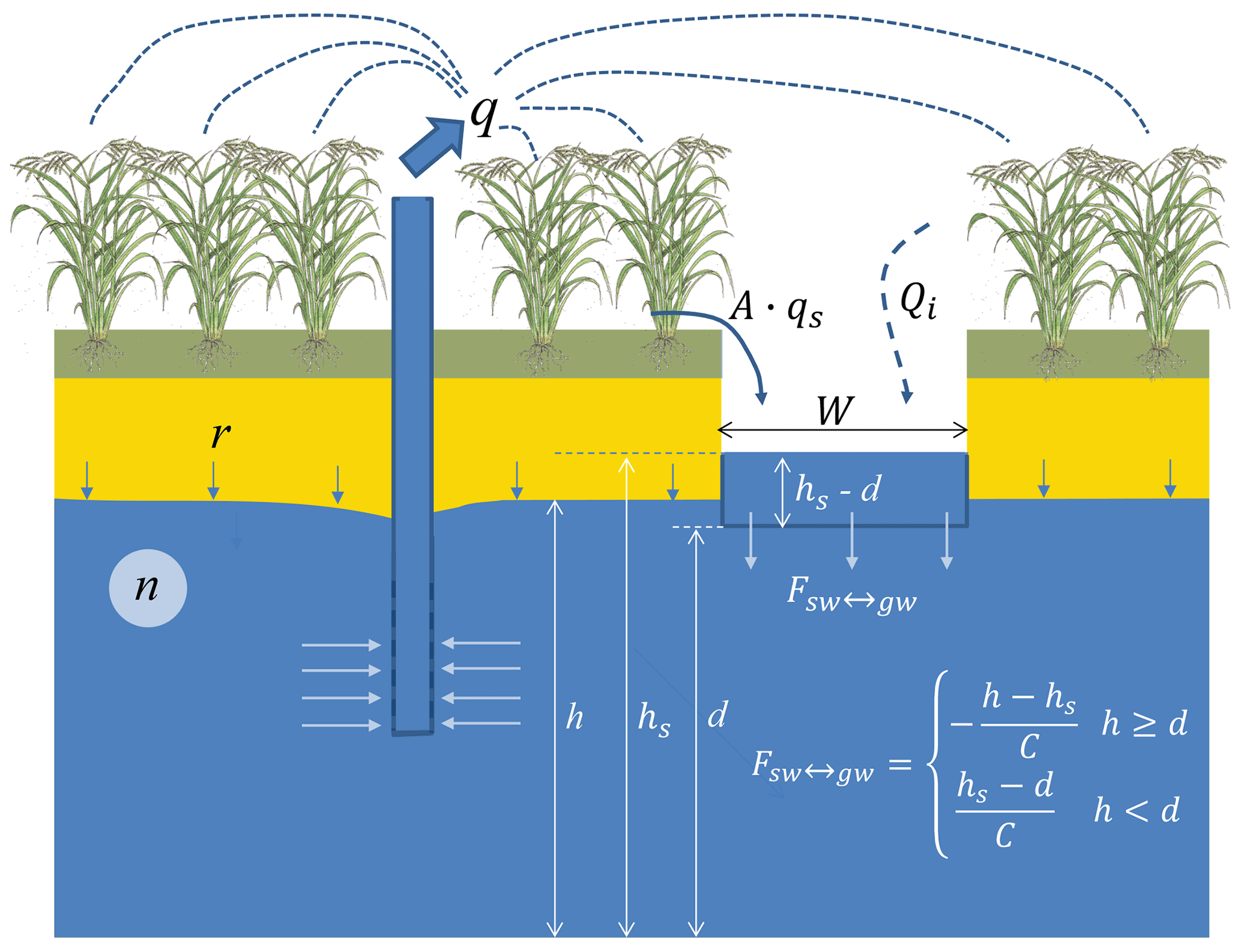
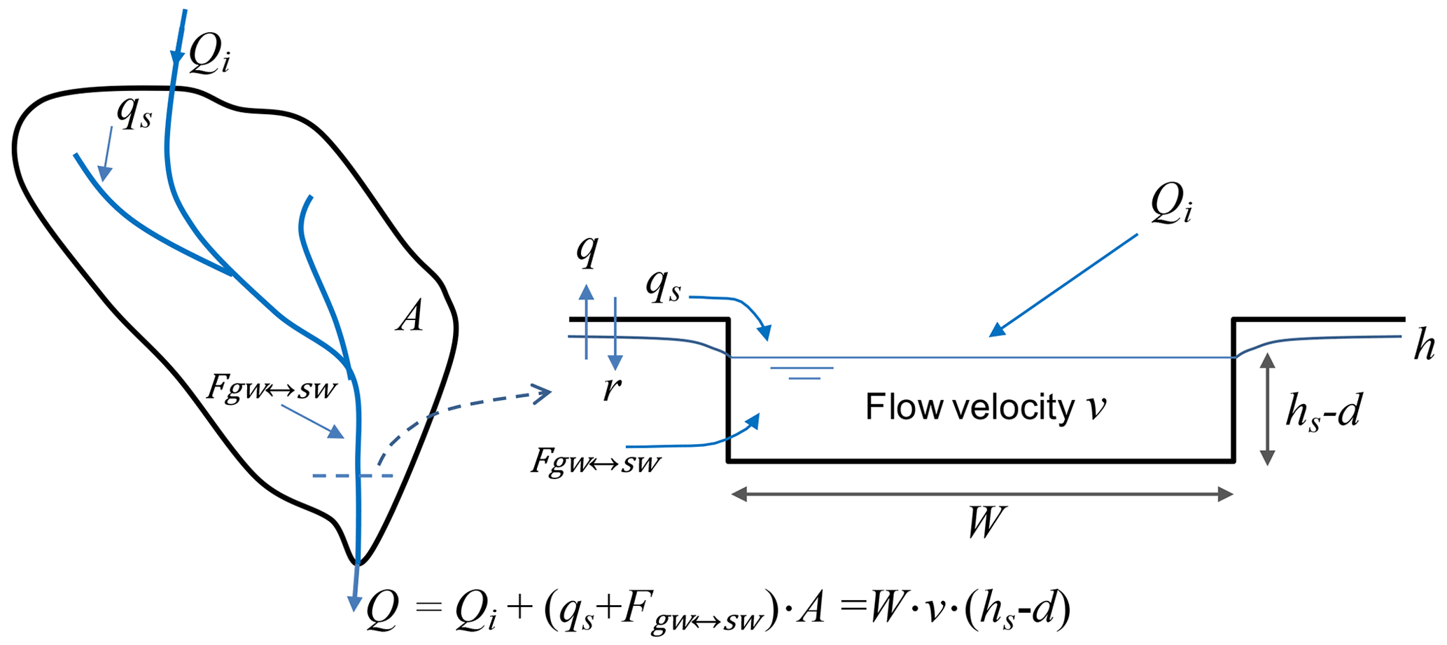
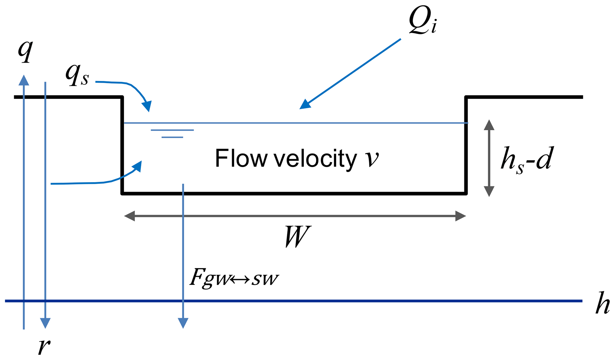
Figure 2Conceptual model of groundwater extracted (in this case for irrigation) from an aquifer recharged by diffuse recharge and riverbed infiltration. Symbols are explained in the text.
A lumped conceptual hydrogeological model is proposed that allows for the analytical treatment of area-average large-scale groundwater decline under varying pumping rates yet exhibits the properties of surface water–groundwater interaction. Consider a simplified model of a phreatic aquifer subject to groundwater pumping (Fig. 2). The volume of groundwater pumped sums up all the pumping efforts of a large number of land owners that all draw water from the same aquifer that can be seen as a common pool resource. Recharge consists of diffuse recharge from precipitation and concentrated recharge from riverbed infiltration, where river discharge comes from local surface runoff and from inflow from upstream areas outside the area of interest.
Being of a lumped nature, the model neglects (lateral) groundwater flow processes within the aquifer and the mutual influence of multiple wells by treating the aquifer as one pool with a given specific yield and unknown depth (i.e. physical limits are unknown) subject to pumping treated as a diffuse sink. The latter is a simplification that represents the effects of hundreds to thousands of wells of farmers spread more or less evenly across the aquifer. Also, we assume withdrawal rate, surface runoff and river bed recharge to be constant in time, neglecting seasonal variations that usually occur due to variation in crop water demand. These simplifications allow us to represent the change in groundwater level h with a simple linear differential equation of the total aquifer mass balance:
with
-
h: groundwater head (m),
-
n: specific yield (–),
-
q: pumping rate per area (m3 m−2 yr−1), and
-
Fgw↔sw: surface water infiltration (or drainage) flux density (m3 m−2 yr−1).
The groundwater–surface water flux is modelled as follows:
where hs is the surface water level and d the elevation of the bottom of the water course. The parameter C is a drainage resistance (yr) which pools together all the parameters of surface–water groundwater interaction, i.e. the density or area fraction of surface waters, surface water geometry, and river bed/lake bed conductance and the hydraulic conductivity of the aquifer. Equation (2) is also used to describe groundwater–surface water interaction in numerical groundwater models such as MODFLOW (McDonald and Harbaugh, 2005) as well as in several large-scale hydrological models (Döll et al., 2014; Sutanudjaja et al., 2018). This is a simplification of the true interaction where in case of a detachment of the groundwater level and the river bed (h<d) negative pressure heads can occur below the river bed and Eq. (2) may underestimate the river bed infiltration (Brunner et al., 2010). However, this latter study also shows that errors remain within 5 % in case the surface water is deep enough (>1 m). Equation (2) provides a critical transition in terms of the effect of pumping on the hydrological system. As long as the groundwater level is above the bottom of the surface water network, the groundwater–surface water flux acts as a negative feedback on groundwater-level decline, at the expense of surface water decline. As the water table falls below the bottom elevation (only possible if the pumping rate q is large enough; see hereafter), surface water decline stops and progressive groundwater decline sets in.
The surface water level itself is a variable which is related to the surface water discharge Q (m3 yr−1) and the groundwater level as follows:
with
-
A: the area over the (sub-)aquifer considered (m2),
-
qs: surface runoff (m yr−1),
-
Qi: influx of surface water from upstream (m3 yr−1),
-
W: stream width (m),
-
d: bottom elevation stream (m), and
-
v: streamflow velocity (m yr−1).
The influx Qi is added to account for aquifers in dry climates where the surface water system is fed by wetter upstream areas, e.g. mountain areas. The surface runoff qs (including shallow subsurface storm runoff) also supplements the streamflow. Equation (3) lumps the streamflow system overlying the phreatic aquifer system with a representative discharge, water height, flow velocity and stream width taken constant in time. Equations (1)–(3) together describe the coupled surface water–groundwater system where all parameters and inputs remain constant with time and groundwater head h and surface water levels hs change over time as a result of groundwater pumping only.
In Appendix A expressions are derived for the following properties of the coupled system.
-
qcrit Critical pumping rate (m3 m−2 yr−1) above which the groundwater level becomes disconnected from the stream.
-
tcrit Critical time (years after start of withdrawal) at which the groundwater level becomes disconnected from the stream, i.e. h<hs.
-
h(t) Groundwater head (m) over time
-
h(∞) Equilibrium groundwater head (m) at t=∞ that only occurs in case q≤qcrit.
-
hs(t) Surface water level (m) over time
-
hs(∞) Equilibrium surface water level (m), which is different when q≤qcrit than when q>qcrit.
-
Q(t) Surface water discharge (m3 yr−1) over time
-
Q(∞) Equilibrium surface water discharge (m3 yr−1), which is different when q≤qcrit than when q>qcrit.
-
qstor(t) Part of the pumped groundwater that comes out of storage, which is different when q≤qcrit than when q>qcrit.
-
qcap(t) Part of the pumped groundwater that comes from capture (reduction in streamflow), which is different when q≤qcrit than when q>qcrit.
Table 1 provides an overview of the mathematical expressions derived for each of these properties in Appendix A. The left column shows the stable regime where upon commencement of pumping after some time an equilibrium is reached with equilibrium groundwater levels h(∞), streamflow Q(∞) and surface water level hs. The middle and right columns show the results of unstable groundwater withdrawal. The behaviour of h(t), Q(t)hs(t) follows that of the stable regime until time t=tcrit, when the groundwater level drops below the bottom of the surface water. After this time the groundwater level h(t) shows a persistent decline, and surface water level hs(t), streamflow Q(t) and fraction of water pumped from capture become constant.
Table 1Overview of derived expressions for groundwater properties used in this paper.
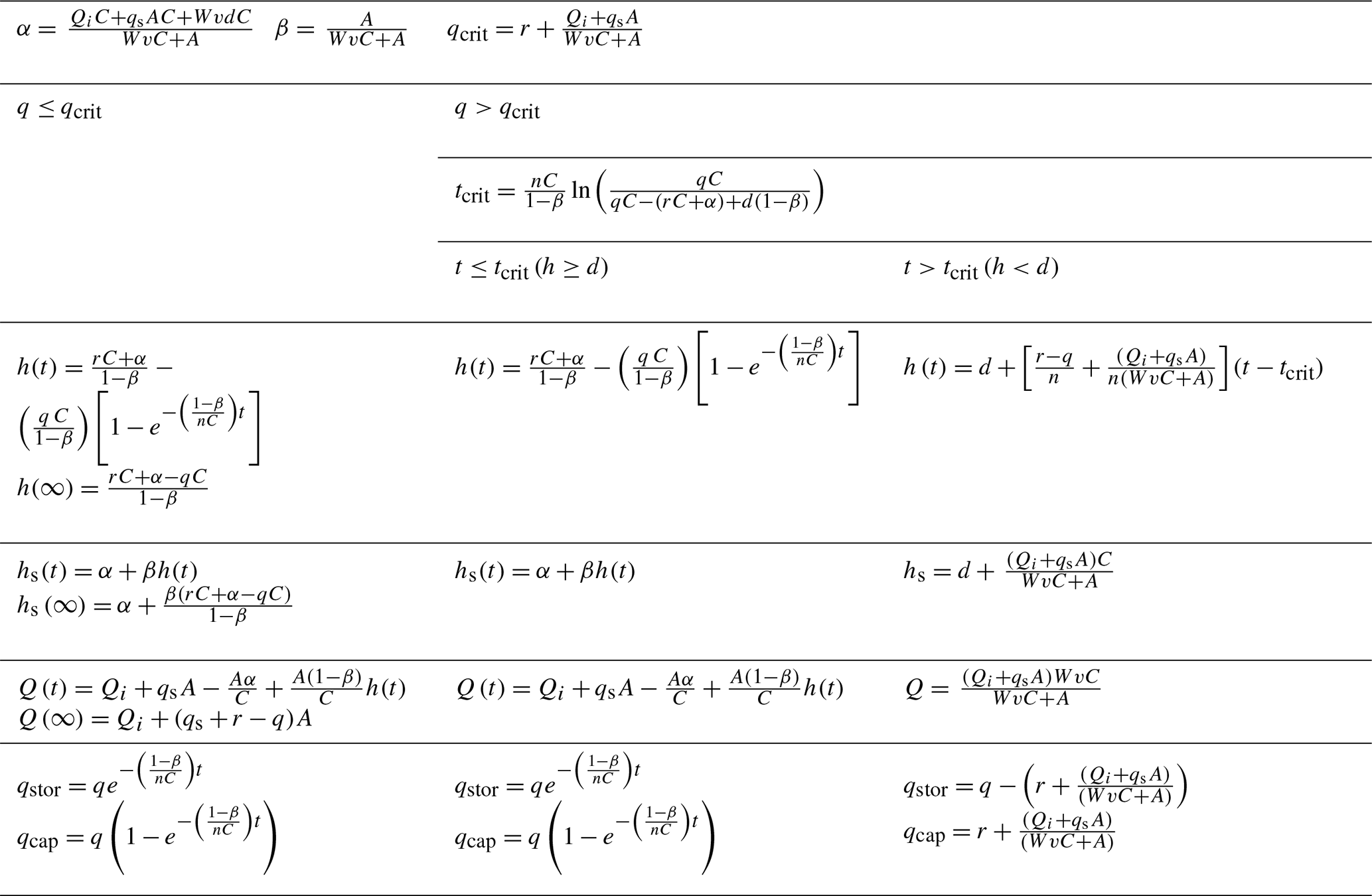
Figure 3 shows the results of a sensitivity analysis for the critical withdrawal rate qcrit and the critical time until the water table disconnects from the stream tcrit. For the stable regime (q≤qcrit) it shows the change in groundwater level at equilibrium , the change in streamflow at equilibrium , and the e-folding time of reaching the equilibrium after the commencement of pumping. For the unstable regime, we show the decline rate of the groundwater level , the (constant) streamflow depletion dQ, and the constant fraction of capture (. We stress that our sensitivity analysis is far from exhaustive (global) and that sensitivity plots are shown to provide a general feel of the behaviour of the model and to show relationships between parameters and outputs that are of interest to show. Unless they are varied on one of the axes, the parameter values used are the reference values denoted in Table 2.
Table 2Reference parameter values used in sensitivity analyses.
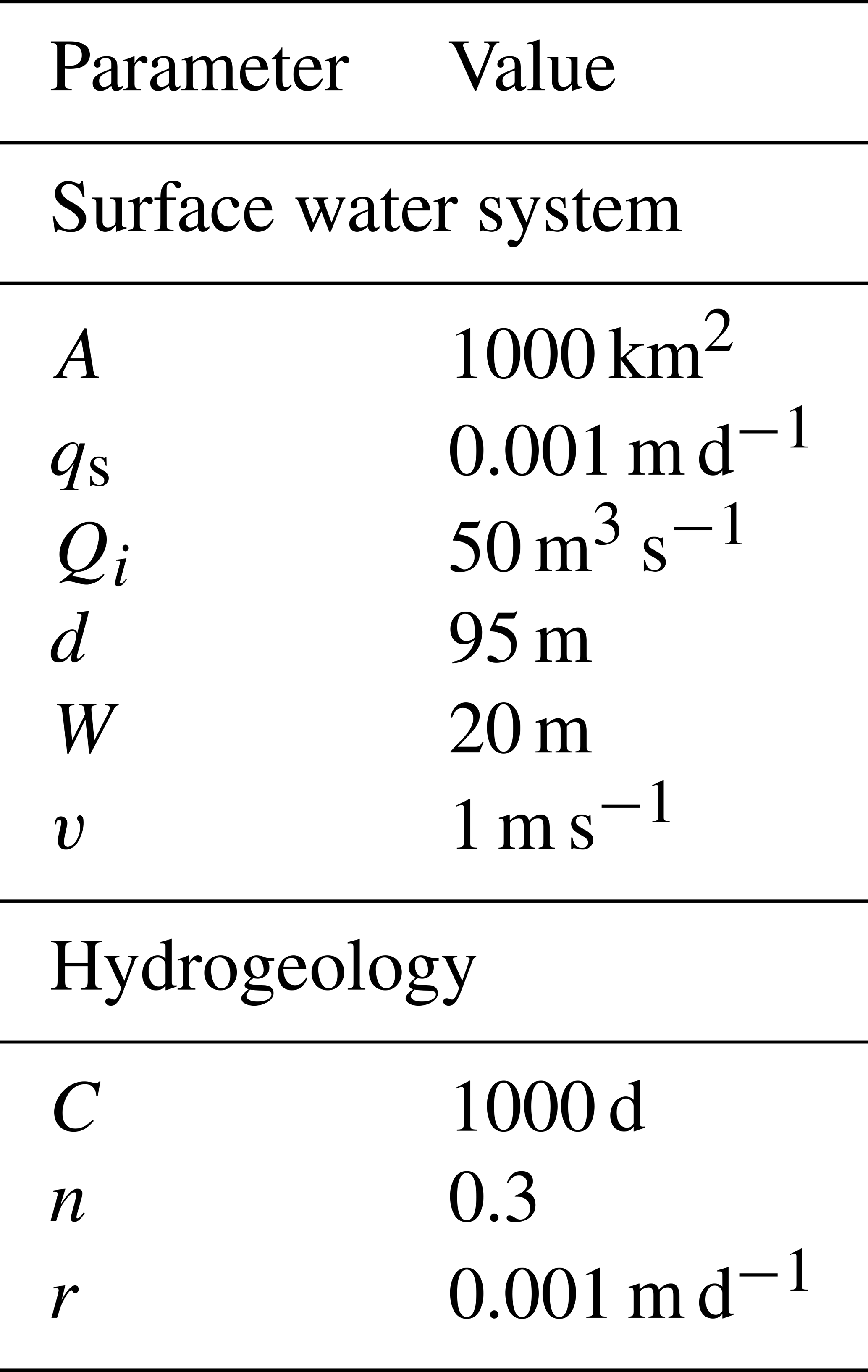
Figure 3a shows that the critical withdrawal rate increases with the relative abundance of surface water due to upstream inflow and runoff and decreases with a decreased strength of the surface water–groundwater interaction (increased value of C). For stable withdrawal rates we see the largest equilibrium groundwater-level declines with increased pumping rates and decreased strength of surface water–groundwater interaction, i.e. decreased capture (Fig. 3c). Figure 3e shows the equilibrium reduction in streamflow to be proportional to groundwater withdrawal rate, as expected, but to depend only mildly on the upstream inflow. The latter is caused by the two-way interaction between surface water and groundwater: increasing inflow for a given withdrawal rate reduces groundwater-level decline, which in turn limits the loss of surface water to the groundwater. As follows from the expression , the time to equilibrium (Fig. 3g), i.e. the time until the pumped groundwater originates completely from capture and no further storage changes occur, is proportional to the resistance value C and the specific yield, where the degree of proportionality depends on the surface water properties. Figure 3g also shows that the time to full capture can be very large, up to several decades.
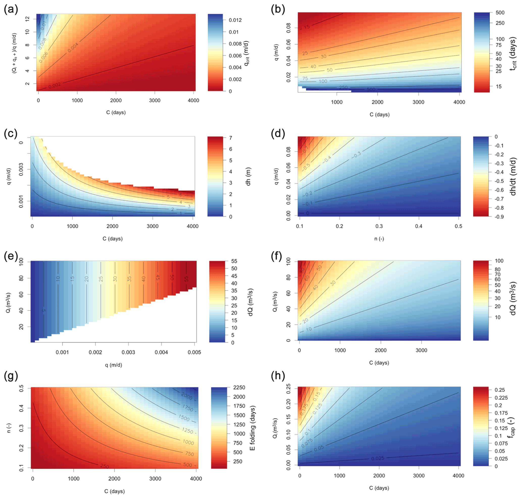
Figure 3Results of the sensitivity analyses showing parameter dependence of qcrit (a) and tcrit (b); variables under stable withdrawal: (c), (e), and ; variables under unstable withdrawal and t>tcrit: (e), dQ (f), and .
Figure 3b–h (right column) provide sensitivity plots of relevant variables in the unstable regime. Figure 3b shows that under the unstable regime, the time tcrit to a transition from a connected to a non-connected groundwater table decreases with withdrawal rate but slightly increases with C. The latter seems counter-intuitive at first, because a larger value of C means reduced surface water contribution and therefore likely larger groundwater-level decline rates and smaller values of tcrit. The equation for h(t) in Table 1 (Eq. A11 in the Appendix) shows that this is indeed the case for early times but that for later times the decline rates are reduced by a larger value of C in the term factor in the exponential. Figure 3d–h show sensitivity plots for t>tcrit (h<d), i.e. groundwater levels are disconnected from the surface water, groundwater is persistently taken out of storage and the capture becomes constant. As expected, the groundwater-level decline rates (Fig. 3d) are proportional to withdrawal rates and inversely proportional to specific yield. The final reduction in streamflow (Fig. 3f) for t>tcrit decreases with the value of C (limited surface water–groundwater interaction), while the availability of surface water is important for smaller values of C. Here, a larger inflow leads to larger losses because losses are proportional to the surface water level which increases with inflow. Figure 3h resembles that of Fig. 3f because apart from the constant recharge, the fraction of capture is proportional to the streamflow reduction which ends up in the pumped groundwater.
4.1 Global parameterization
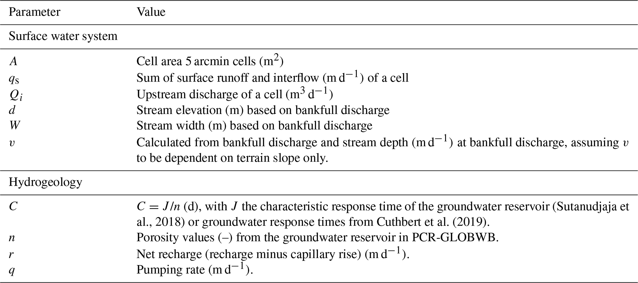
We applied the analytical framework to the global scale at 5 arcmin resolution (approximately 10 km at the Equator) by obtaining parameters and inputs from the global hydrology and water resources model PCR-GLOBWB 2 (Sutanudjaja et al., 2018; see Table 3 and Figs. S1–S9 in the Supplement (https://doi.org/10.4121/uuid:e3ead32c-0c7d-4762-a781-744dbdd9a94b, last access 22 October 2020). For the flux densities q, qs, r, the discharge Qi, and the velocity v, we used the average values over the period 2000–2015. Note that for an application of the analytical framework on a cell-by-cell basis, the reduction in streamflow dQ in a given cell should be accounted for by reducing the inflow Qi to the downstream cell. However, by using as inflow Qi the upstream discharge from a PCR-GLOBWB simulation that includes human water use, upstream withdrawals from surface water and groundwater are already accounted for. Note that they would also be implicitly included in case an observation-based streamflow dataset (e.g. Barbarossa et al., 2019) would have been used for Qi. The groundwater–surface water interaction parameter C is determined from the characteristic response time J of the groundwater reservoir in PCR-GLOBWB 2, which is based on the drainage theory of Kraijenhoff-van de Leur (1958). From this solution and Eq. (2) it can be shown that C=J/n (see Appendix B). Since the variables qcrit and tcrit depend heavily on the value of C, we have also included the dataset of groundwater response time published by Cuthbert et al. (2019) (https://doi.org/10.6084/m9.figshare.7393304 (last access: 22 October 2020) to calculate the C value.
Table 3Parameter and input values used in global-scale analyses at 5 arcmin cells (∼ 10 km at the Equator). All inputs obtained from PCR-GLOBWB 2 (Sutanudjaja et al., 2018), except the C values obtained from PCR-GLOBWB and from Cuthbert et al. (2018); input variables averaged over the period 2000–2015.
4.2 Global results
Figure 4 shows the groundwater depletion rates q−qcrit for the areas with unstable groundwater withdrawal. The resulting patterns are similar to those calculated from previous global studies (Wada et al., 2012; Döll et al., 2014) and show the well-known hotspots of the world. Total depletion rates in Fig. 4 are 158 km3 yr−1 (a) and 166 km3 yr−1 (b), which are in the range of previous studies, e.g. 234 km3 yr−1 (Wada et al., 2012; year 2000), 171 km3 yr−1 (Sutanudjaja et al., 2018; 2000–2015), and 113 km3 yr−1 (Döll et al., 2014; 2000–2009).
The similarity of the groundwater depletion estimates to those obtained from global hydrological models can be explained by the fact that the way the groundwater–surface water system is modelled in Fig. 1 is similar to how the groundwater reservoirs and their interactions with surface water have been implemented in global hydrological models such as PCR-GLOBWB (De Graaf et al., 2015) and WGHM (Döll et al., 2014) (see also Appendix B). Since the groundwater dynamics of the latter models are (piece-wise) linear and groundwater recharge in our model is applied directly in Eq. (1) – i.e. the non-linear responses of the soil system to precipitation and evaporation are bypassed – forcing our model with average fluxes r,q, Qi, and qs and using the parameter J from PCR-GLOBWB yields almost the same depletion rates as from the time-varying model simulations with PCR-GLOBWB. The small difference between our estimate (158 km3 yr−1) and the value from PCR-GLOBWB 2 (Sutanudjaja et al., 2018) (171 km3 yr−1) is explained by a resulting non-linearity not accounted for: during dry periods some of the streams in the PCR-GLOBWB run dry and do not contribute to the concentrated recharge flux. It should be noted that our results are obtained at only a fraction of the computational costs of global hydrological models: a few minutes at a single PC compared to 2 d on a 48-core machine with PCR-GLOBWB at 5 arcmin. Thus, the sensitivity to changing pumping rates or changes in recharge under climate change can be quickly evaluated.

Figure 4Average groundwater depletion rates (q−qcrit) over 2000–2015 at 5 arcmin resolution calculated with the data from Table 2. (a) Using C values from Sutanudjaja et al. (2018); (b) using C values based on Cuthbert et al. (2019); (c) difference map (a–b).
Figure 5 shows the time to critical transition tcrit from both datasets. It is quite striking that, although the depletion rates are rather similar between datasets (Fig. 4), the critical transition times are much larger for the Cuthbert et al. (2018) dataset. These differences can even add up to 2–3 orders of magnitude, which is extremely large. The reason is that the characteristic response times based on Cuthbert et al. (2018) are much larger (also up to 2–3 orders of magnitude) than those based on PCR-GLOBWB. Since the e-folding time in the stable regime is close to proportional to the C value (e.g. Fig. 3g), this is also true for the critical transition time. The very large differences in response times between these two datasets reveal that our method is only as good as its inputs and that critical transition times and times to full capture calculated with our approach should be interpreted with care and as order of magnitude estimates at best.
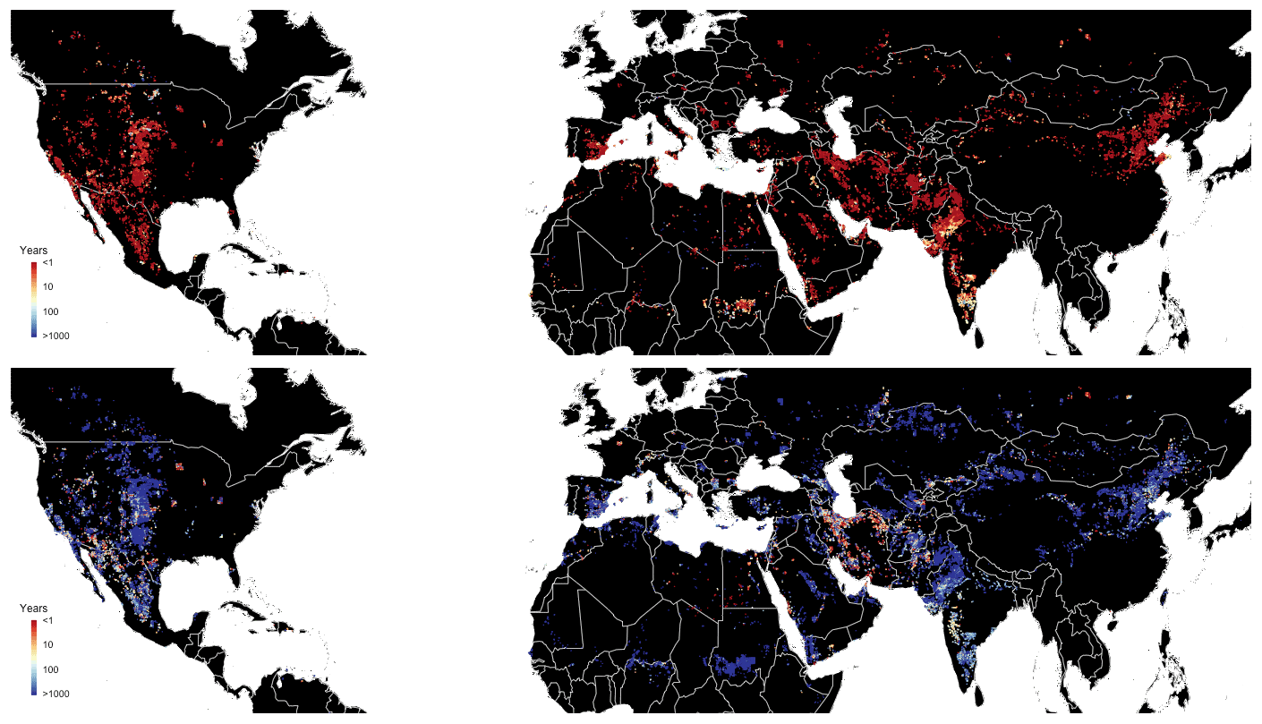
Figure 5Critical transition times (critical time at which the groundwater level becomes disconnected from the stream after start of pumping, i.e. h<hs in case q>qcrit) calculated with the data from Table 1. The top figure uses C values from Sutanudjaja et al. (2018) and the lower figure from Cuthbert et al. (2019).
To further explore the global impacts of groundwater withdrawal, we calculated relevant output variables for the areas that have been identified as subject to stable groundwater withdrawal (q≤qcrit; Fig. 6) and unstable withdrawal (q>qcrit; Fig. 7). Figure 6a shows the equilibrium water table decline from stable groundwater withdrawal. We see the largest declines occurring in areas with larger groundwater withdrawals, which are often close to the depletion areas (Fig. 4) and coincide with regions with limited surface water occurrence due to a semi-arid climate (higher C values). In contrast, the equilibrium decline in streamflow (Fig. 6b) is focused in areas with significant groundwater withdrawal and higher surface water densities (low C values), which are those areas that have a more semi-humid climate where both groundwater use and surface water use are present. These are also the areas with relatively short times to equilibrium (Fig. 6c).
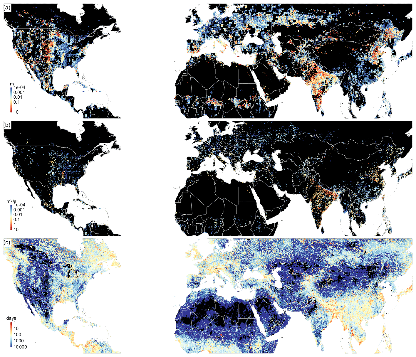
Figure 6Results for the areas with stable withdrawal rates (q≤qcrit); (a) equilibrium groundwater-level decline (m); (b) equilibrium reduction of discharge (m3 s−1); (c) e-folding time to complete capture; black areas are areas without groundwater withdrawal, with unstable groundwater withdrawal or negligible values ().
As expected, the groundwater decline rates under unstable withdrawal (Fig. 7a) mirror the depletion rates (Fig. 4). Estimates based on piezometers for major depleting areas are on the order of 0.4–1.0 m yr−1 in southern California and the Southern High Plains aquifer (Scanlon et al., 2012) and 0.1–1.0 m yr−1 in the Gangetic Plain (MacDonald et al., 2016). Our estimates are at the lower end of those observed ranges, which could be partly explained by the fact that, particularly in the US, groundwater withdrawal is from semi-confined aquifers, leading to a larger head decline per volume out of storage than follows from the specific yields used in our conceptual model. The largest change in streamflow and the highest fraction of capture are found in areas where groundwater depletion coincides with the presence of surface water, e.g. such as the northern and eastern parts of the Ogallala aquifer, the Indus basin and southern India.

Figure 7Results for the areas with unstable withdrawal rates (q>qcrit); (a) groundwater-level decline rate (mm yr−1); (b) equilibrium reduction of discharge (m3 s−1); (c) fraction of capture (–); black areas are areas without groundwater withdrawal, with stable groundwater withdrawal or with negligible values ().
4.3 Sensitivity and evaluation of global results
Critical parameters that determine the stream–aquifer interaction and hence many of the outputs shown in Figs. 4–7 are the stream–aquifer resistance parameter C and the stream bottom elevation d. We performed a local sensitivity analysis by changing the parameters C and d±10 % around their current values (Figs. S3 and S6) and calculated the relative change in the output per unit relative change in parameters C and d. The results (Table S1) reveal that for most outputs the sensitivity to C and d is limited (below unity). A notable exception is the sensitivity of tcrit to d, which can be quite large, particularly for the lower values of C from Sutanudjaja et al. (2018). From the sensitivity analysis we conclude that the global results are relatively robust to changes in the parameters C and d, except for the critical time to stream–aquifer disconnection, which is sensitive to d and to a lesser extent to C.
To evaluate our global results, we compare these with observations and model results at various scales, working from large to smaller scales (both in extent and resolution). These include aquifer average storage change from the Gravity Recovery and Climate Experiment (GRACE) satellite, global-scale groundwater and streamflow depletion estimates from a global groundwater model (De Graaf et al., 2019), continental-scale (conterminous US) groundwater and streamflow depletion estimates from Parflow-CLM (Condon and Maxwell, 2019) and groundwater flow and streamflow decline rates for the Republican River Basin based on in situ observations (Wen and Chen, 2006; McGuire, 2017).
From the results in Fig. 4a (with C from Sutanudjaja et al. (2018), assuming q>qcrit and t>tcrit) we computed average depletion rates of the world's major aquifers subject to depletion (following Richey et al., 2015) and compared these with average trends in total water storage (TWS) from GRACE gravity anomalies over the period 2003–2015 (Fig. 8). We used the JPL GRACE Mascon product RL05M (Wiese, 2015; Watkins et al., 2015; Wiese et al., 2016) (https://doi.org/10.5067/TEMSC-OCL05, last access: 22 Ocotober 2020). We did not correct TWS for changes in other hydrological stores, assuming the latter to be approximately constant over a 13-year period in semi-arid areas with limited surface water and TWS trends to mainly reflect groundwater depletion. Figure 8 shows that the estimated depletion rates are reasonably consistent with the GRACE estimates, particularly for the known hotspot aquifers with the largest depletion. Notable exceptions are an overestimation of the depletion rate in the Paris Basin and underestimation of depletion rates of the Maranhao Basin, the North Caucasus Basin and the North African Aquifer Systems. These differences may be caused by errors in withdrawal data from PCR-GLOBWB 2 (Fig. S9), errors in streamflow leakage and errors that result from not correcting the GRACE products for possible secular trends in other hydrological stores. A notable effect could be that by assuming aquifers to be unconfined, we overestimate the leakage from surface water to groundwater in pumped confined aquifers, leading to an underestimation of depletion rates. It should also be noted however that the aquifers whose depletion rates are underestimated have estimated GRACE trends between 1 and 10 mm yr−1, just above the accuracy limit of GRACE TWS trends (viz. Richey et al., 2015).
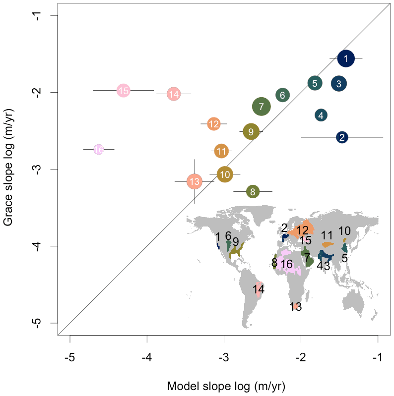
Figure 8Comparison of depletion rates in Fig. 4a for major groundwater basins with average depletion rates from GRACE (m yr−1). The size of the circles is proportional to aquifer area; crosses are standard errors in estimated mean aquifer trends. 1: Central Valley (California); 2: Paris Basin; 3 Ganges–Brahmaputra Basin; 4; Indus Basin; 5: North China Plain; 6. Ogallala (High Plains) Aquifer; 7. Arabian Aquifer System; 8: Senegalo–Mauritanian Basin; 9: Atlantic and Gulf Coastal Plains Aquifer; 10: Songliao Basin; 11: Tarim Basin; 12; Russian Platform basins; 13: Karoo Basin; 14: Maranhao Basin; 15: North Caucasus Basin; 16: North African Aquifer systems.
At the global scale, we compared the head decline rate (mm d−1) calculated with the analytical framework with average decline rates over the period 2000–2015 as obtained from the global groundwater model of De Graaf et al. (2019). Note that we restricted this comparison to the areas with unstable withdrawal rates (q>qcrit, t>tcrit). The results shown in Fig. S10 show that the patterns of high and low values of the two estimates are similar but that the estimated decline rates from our analytical framework are larger than those estimated by De Graaf et al. (2019). The most likely cause of the larger values in our approach is that it neglects the impact of lateral flow (across cell boundaries) or that the J value of PCR-GLOBWB used to calculate the C parameter (see Appendix B) is too large, so that leakage from the streams is underestimated. Comparison of the stream depletion estimates from the analytical framework (see Fig. S11, assuming q>qcrit, t>tcrit or q<qcrit, t≫tef) shows similar patterns to that of De Graaf et al. (2019) but also slightly larger values. Thus, the most likely cause of the larger depletion values of our analytical framework (Fig. S10) is the neglect of lateral flow between cells.
At the continental scale, we compared groundwater storage changes (m) and stream depletion (% of mean annual flow) across part of the conterminous US obtained from a ParFlow-CLM model (Condon and Maxwell, 2019) with the global estimates from our analytical framework. ParFlow simulates coupled groundwater and surface water flow by solving the 3D Richards equation and the diffusive wave equation respectively, while the community land model (CLM) includes land surface processes such as evaporation, plant water use, snow accumulation and snowmelt. Condon and Maxwell (2019) calculate the total effects of pumping from the pre-development stage (1900 until 2008), while our global results are based on the average withdrawal rates for the period 2000–2015. To make our results comparable with those of Condon and Maxwell (2019), we took their reported total storage loss of 1000 km3 since 1900 and determined the period length for which the total groundwater withdrawn based on Sutanudjaja et al. (2018) across the US approximately equals 1000 km3. This resulted in the period 1965–2015. We subsequently recalculated the global maps using the average groundwater withdrawal rate over 1965–2015 from Sutanudjaja et al. (2018).
The results are shown in Fig. S12 (for q>qcrit, t>tcrit) and Fig. S13 (q>qcrit, t>tcrit or q<qcrit, t≫tef). Figure S12 shows again that the analytical approach yields larger depletion estimates than ParFlow, but the results are more similar than with the global model of De Graaf et al. (2019). It is speculative at best to explain why the results of Condon and Maxwell (2019) are more similar. One possible explanation may be that the overestimation of decline rates due to ignoring lateral flow between cells in our approach is partly offset by the neglect of headwater streams falling dry under continuous pumping. This effect is included in ParFlow-CLM, which results in larger head decline rates that are closer to ours. The global groundwater model of De Graaf et al. (2019) does not include this effect as streams in this model remain water-carrying even if the groundwater level drops below the stream bottom elevation.
Figure S13 (top) shows the percentage reduction of streamflow by groundwater pumping since pre-development as calculated by ParfFlow-CLM and Fig. S13 (bottom) the estimates based on the analytical framework. We show both maps for reference in the Supplement, but it turns out that comparing the streamflow reduction of the analytical framework with that of ParfFlow-CLM is inhibited by differences in model output and presentation. The ParfFlow-CLM results represent cumulative dQ as a fraction of Q, whereas the results from the analytical framework represent marginal dQ as a fraction of Q, which makes the results only comparable for the headwater catchments. Also, the difficulty of comparison due to the resolution gap (ParfFlow-CLM: 1 km; analytical framework: 5 arcmin, ∼ 10 km) is exacerbated due to the different map formats (vector vs. raster). Therefore, we refrain from further comments and show the maps as they are.
At the basin scale, we compared our global results with trends in groundwater head decline and streamflow decline as obtained from observations of groundwater levels and surface water discharge in the Republican River Basin (USA). The Republican River Basin runs through the northern part of the High Plains aquifer system, which is heavily influenced by groundwater withdrawal. We used data from a study by Wen and Chen (2006) that estimated trends in streamflow over the period 1950–2003 for 24 gauging stations spread across the Republican River and its tributaries. The trends were adjusted for possible trends in precipitation and are therefore assumed to only reflect a decrease in streamflow as a result of groundwater pumping. This resulted in 18 out of the 24 stations with significant negative trends. Wen and Chen (2006) also provide groundwater-level observations from three wells with filters in the Ogallala formation at three locations positioned in three representative locations in the Republican River Basin. We used the analytical framework with global parameters (Table 3) but with the average values of q, qs, r, and Qi over the period 1960–2003 obtained from PCR-GLOBWB (Sutatudjaja et al., 2009) to estimate at 5 arcmin resolution average groundwater-level decline rates (m yr−1). Figure S14 in the Supplement shows boxplots of streamflow trends and groundwater head trends from the observations and from our framework. The distribution of estimated streamflow decline overlaps with that from the observed trends with a slight underestimation. The observed groundwater head decline rates however are underestimated. This may be caused by the fact that we only have three observations, which are from a mostly confined aquifer where small storage coefficients lead to larger decline rates.
To further investigate the performance of our method in reproducing groundwater-level declines at the sub-basin scale, we compare estimated groundwater-level declines between 2002 and 2015 from 1522 groundwater wells in the Republican River Basin obtained from McGuire (2017) (https://pubs.er.usgs.gov/publication/sim3373, last access: 25 May 2021). Figure S15 shows maps and boxplots of observed groundwater-level declines (m) and declines estimated from the analytical framework. Although the overall pattern of groundwater depletion in the Republican River Basin is reproduced, there are occasional outliers in the global estimates that are not seen in the observations. This is likely the result of the global withdrawal data that are obtained by downscaling the total US groundwater withdrawal to 5 arcmin based on 5 arcmin estimates of total groundwater demand (Sutanudjaja et al., 2018). Although these downscaled withdrawal rates are well verified at the county scale (see Wada et al., 2012), the mismatch at the 5 arcmin scale can be large. Thus, when using global datasets, the analytical framework is limited to the sub-basin scale and is too coarse for local-scale estimates. Improvements can be expected when local data on groundwater withdrawal are available at finer resolution.
4.4 Critical limits to groundwater withdrawal for major basins
We finish the result section by summarizing critical limits to groundwater withdrawal for the major river basins of the world. In Fig. 9a the median value of qcrit is plotted for the major basins in the world (sub-watershed level of HydroBasins, Lehner et al., 2008) together with the areas where groundwater withdrawal is on average unstable over the years 2000–2015. This figure provides, at first order, a global map of the maximum limit to physically stable groundwater withdrawal rates. The parts of the world where the critical withdrawal rates are very small largely coincide with the band of countries that experience high values of water stress (Hofsté et al., 2019). This shows that there is little room in these areas to supplement water demand without causing groundwater depletion.
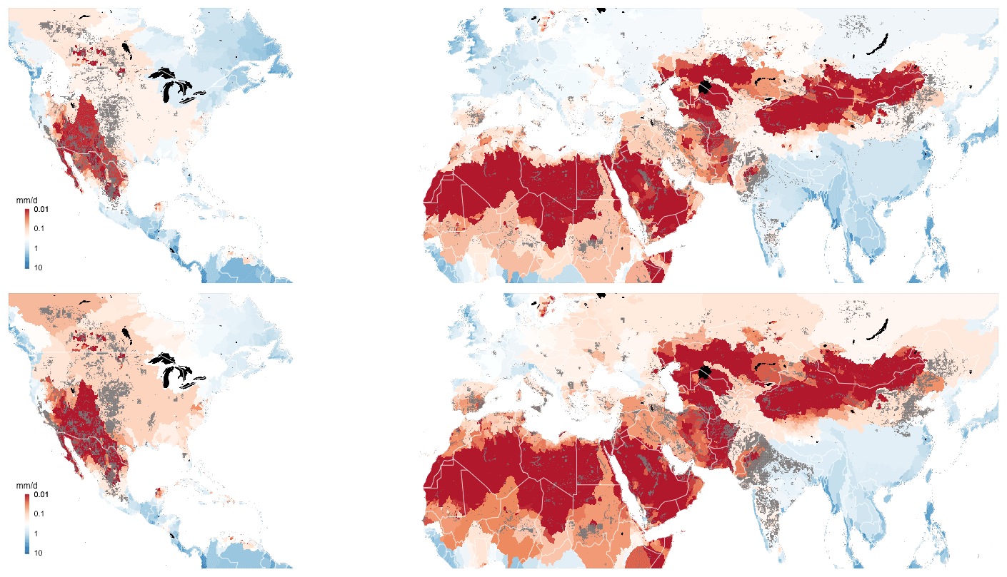
Figure 9Global limits to stable groundwater withdrawal rate. Top: limit to physically stable groundwater withdrawal mapped as the median qcrit per sub-basin (based on HydroBasins: Lehner et al., 2008); grey-shaded areas are those for which q>qcrit; bottom: limit to ecologically stable groundwater withdrawal mapped as the median qeco per sub-basin; grey-shaded areas are those for which q>qeco.
The ecological limits to groundwater withdrawal, qeco, can be defined as the withdrawal rate that is low enough to prevent streamflow from dropping below some environmental flow limit Qenv, i.e. a value that is high enough to safeguard the integrity of the aquatic ecosystems (Linnansaari et al., 2013; Pastor et al., 2014). The value of qeco can be calculated by inverting Eq. (A14) and taking Q(∞)<Qenv:
We note that environmental flows are usually defined during low-flow conditions (Pastor et al., 2014; Gleeson and Richter, 2018), so it may be more appropriate to use the value of Q(∞) as the average over the summer half year instead of yearly averages. If we assume that the average streamflow regime follows a cosine function with a period of 1 year, then the average (natural) streamflow Qs in summer would be equal to
and qeco becomes
In Fig. 9 (bottom) we have plotted qeco using, as an example, Qenv as 20 % of the average natural summer streamflow Qs. The resulting map can be seen as a first-order approximation of the limits to ecologically stable groundwater withdrawal. In most cases, qeco<qcrit, as is also evident from the larger grey-shaded areas in the bottom figure compared to the top figure. The results suggest that supplementing water demand by groundwater use in the world's water-stressed areas is limited under ecological constraints. We stress that the sub-basin-scale critical and environmental limits are meant for large-scale environmental assessment, not for local groundwater management.
We have introduced an analytical framework based on a lumped conceptual model that intends to describe to what extent groundwater withdrawal affects groundwater heads and streamflow under changing regimes of groundwater–surface water interaction. By feeding the framework with the parameters and inputs from a more complex hydrological model (i.e. PCR-GLOBWB), it can be used as a screening tool for regional-scale groundwater sustainability, i.e. by providing a rich tableau of hydrologically and ecologically relevant outputs at very limited computational costs. Another possible application is in hydro-economic modelling, where the equations in Table 1 can be used as regionally varying hydrological response functions (Harou et al., 2009; MacEwan et al., 2017) in hydro-economic optimization – where model evaluations need to be fast – in order to infer socially optimal pumping rates that include environmental externalities.
The estimated global groundwater and surface water depletion rates were compared with observations and model results at various scales (support and extent), with mixed but overall favourable results up to the sub-basin scale. Results show that the analytical framework provides similar results to those of global hydrological models but tends to overestimate the groundwater depletion rates from groundwater flow models that account for lateral flow between cells. Also, without calibration, the critical transient times, i.e. the time from commencement of pumping till the detachment of the water table from the stream, as well as the related time to full capture, are order-of-magnitude estimates at best. Finally, when using global datasets, the analytical framework is limited to the sub-basin scale and is too coarse for local-scale estimates.
We stress that output variables that are related to critical environmental limits such as qcrit, qeco, tcrit and tef are difficult to validate directly, particularly at the larger scales at which our framework operates. This would require large-scale pumping experiments or metering of pumping wells in basins while surface water and groundwater are intensively monitored over decades. As such, the critical limits are non-observables calculated with a model that is only partly validated with a limited set of output variables, i.e. groundwater-level decline and streamflow depletion. We note however that this limitation is not restricted to our analytical framework but occurs for any analytical or numerical groundwater model used.
Clearly, many complicating factors are neglected in our approach, e.g. underground spatial heterogeneity, including the occurrence of multiple aquifer systems and semi-confined layers that are present in many important alluvial groundwater basins, the variable depth and topology of the surface water system and the intermittent nature of many streams in semi-arid to semi-humid areas, and the locations of the wells with respect to the streams. Of these, the neglect of confining layers may be one of the more crucial limitations of the approach. For instance, a considerable part of the groundwater used for irrigation in the big alluvial basins of the US (e.g. Ogallala and Central Valley of California), where farmers have the financial resources to drill deep wells (Perrone and Jasechko, 2019), is pumped from deeper confined aquifers. This means that the groundwater–surface water interaction is limited to the large rivers and lakes only and that head decline per volume water pumped is larger than in phreatic conditions. It would in principle be possible to include the effect of a confining layer by using a larger value of the groundwater–surface water resistance parameter C, a smaller value of recharge r and a storage coefficient instead of specific yield. Similarly, the impacts of seasonably variable boundary conditions of q, qs and Qi could be taken into account by simple convolution, considering that the groundwater-level responses h(t) and dh/dt (Table 1) are respectively step and impulse responses of a linear system. Also, the effects of multiple streams with variable stream bottom elevations could be included by extending the piecewise linearization of Eq. (2) to more domains (e.g. Bierkens and te Stroet, 2007). However, we argue that such extensions are not in the spirit of the simple analytical framework developed, which intends to provide first-order sensitivities at larger scales. If the addition of complexity is needed to provide more accurate assessments for a specific case, it would be more logical to build a tailor-made numerical groundwater flow model.
We end with the note that a global application of our conceptual analytical framework is not restricted to the use of data from the PCR-GLOBWB repository. The necessary fluxes r, q, Qi and qs can also be obtained from other repositories of multi-model re-analyses such as EartH2Observe (Schellekens et al., 2017) and from the combination of remotely sensed estimates of hydrological variables (Lettenmaier et al., 2015; McCabe et al., 2017), e.g. estimating recharge and surface runoff from remotely sensed precipitation, evaporation and soil moisture change and using high-resolution global datasets on discharge (Barbarossa et al., 2018) and river bed dimensions (Allen and Pavelsky, 2018; Lehner et al., 2018).
A1 Basic equations
We repeat the three basic equations that make up the lumped conceptual model of regional-scale groundwater pumping with groundwater–surface water interaction.
The groundwater head as described with the total aquifer mass balance is
The groundwater–surface water flux is
The surface water balance is
A2 The cases h(t)≥d and q<qcrit
We will start by analysing the case where h≥d, i.e. where the groundwater level is attached to the surface water body. We further assume that q<qcrit, i.e. the groundwater withdrawal, is such that the groundwater level never falls below the surface water bottom level d. In this case, the surface water flux Q (m3/d) is related to the groundwater and surface water level as follows (see Fig. A1):
with
-
A: the area over the (sub-)aquifer considered (m2),
-
qs: surface runoff (m yr−1),
-
Qi: influx of surface water from upstream (m3 yr−1),
-
W: stream width (m),
-
d: bottom elevation stream (m), and
-
v: streamflow velocity (m yr−1).
Collecting hs on one side and the other terms on the right-hand side results in the following relation between surface water height and groundwater head:
with
From Eqs. (A1) and (A2) the differential equation for groundwater level gives
After substituting Eq. (A5),
From Eq. (A9) follows the steady-state groundwater level under natural conditions (q=0 and ):
Solving differential Eq. (A9) for initial condition Eq. (A10) then yields
which also gives the equilibrium groundwater level for t→∞:
The surface water level with time is given by Eq. (A5) and the final equilibrium surface water follows from Eqs. (A5) and (A12) as
The surface water discharge as a function of time follows from combining Eqs. (A3) and (A5):
with h(t) given by Eq. (A11). The equilibrium discharge is obtained by substituting Eq. (A12) for h(∞) into Eq. (A14):
which also follows logically from the water balance.
A3 The critical withdrawal rate qcrit
The critical withdrawal rate determines whether at larger times the water table drops below the bottom of the surface and moves to the physically unstable regime. We seek q such that h(∞)=d:
from which follows
Substituting α and β yields, after some manipulation,
A4 Critical transition time tcrit in case q>qcrit
In case q>qcrit at some time after pumping (tcrit), the groundwater level will fall below the bottom elevation d of the surface water. Before that time, it follows the water table decline according to Eq. (A11). So, we can find tcrit by solving it from
Solving an equation of the form gives as a solution , from which follows, from Eq. (A19),
A5 The cases q>qcrit and t>tcrit (h(t)<d)
In case the water table is below the bottom elevation of the stream, the water balance of the stream reads as (see Fig. A2)
from which we can derive an equation for the minimum and constant elevation of the surface water level (valid for t>tcrit):
The differential equation describing the change in groundwater with time now becomes
Substituting hs−d from Eq. (A22) then yields an equation for the groundwater decline rate:
which is always negative since q>qcrit. With initial condition h(tcrit)=d, one obtains from Eq. (A24) an equation for h(t)t> tcrit:
A6 Sources of pumped groundwater: q<qcrit or t<tcrit (h(t)≥d)
When neglecting direct evaporation from groundwater, the sources of pumped groundwater in case q<qcrit either come out of storage or from recharge that does not contribute to streamflow. The latter is called “capture”. From the water balance Eq. (A1), we thus find
The first two terms constitute the water pumped from capture (with Fgw↔sw negative in case h>hs and positive when h<hs) and the second term the water out of storage. Furthermore, from differentiation of Eq. (A11) we have
Combining Eqs. (A27) and (A26) then gives (since capture + out of storage adds up to q):
This shows that the fraction groundwater taken out of storage reduces over time until head decline stops and all water comes out of capture.
A7 Sources of pumped groundwater: q>qcrit and t>tcrit (h(t)<d)
In case of q>qcrit and t<tcrit, the sources of pumped groundwater follow Eq. (A28). After the groundwater table falls below the bottom elevation of the stream and t>tcrit, the sources of water follow from Eq. (A24):
Therefore,
Since the third term is the storage change and capture plus storage change adds up to q, we have
which shows that at after t>tcrit the ratio of pumping from capture (i.e. recharge and surface water leakage) and storage change becomes constant.
In PCR-GLOBWB 2 (Sutanudjaja et al., 2018) and in similar global hydrological models, the relationship between groundwater discharge Qg (m3 m−2 d−1) and the volume Vg (m3/m2) stored in the groundwater store is given by a simple linear relationship
with J the characteristic response time of the groundwater system (e-folding time of the recession) (yr). In some of the global models J is obtained by calibration to low flows or recession curves. In PCR-GLOBWB it is calculated from the transient drainage theory of Kraijenhoff-van de Leur (1958) as
with n the drainable porosity or specific yield, L the average distance between water courses (derived from the drainage density per cell) and T the aquifer transmissivity obtained from global hydrogeological datasets (e.g. Gleeson et al., 2014). A similar approach was used by Cuthbert et al. (2019) to derive groundwater response times.
The drainable volume of groundwater stored in the groundwater reservoir (m3 m−2) of a grid cell of a global hydrological model can also be expressed as , with hs the surface water level and h the groundwater level in the cell. Substituting this into Eq. (B1), we obtain the equivalent groundwater drainage equation for a grid cell:
Comparing Eqs. (B3) with (A2) shows that to obtain the same groundwater–surface water exchange in the global hydrological model and the conceptual analytical model, we must have
Note that these relationships assume that the streams remain connected with the surface water, which is not entirely consistent with Eq. (A2).
The data used in the global assessments provided by PCR-GLOBWB 2 can be downloaded from https://doi.org/10.4121/uuid:e3ead32c-0c7d-4762-a781-744dbdd9a94b (last access: 22 October 2020, Sutanudjaja et al., 2018). The groundwater response times of Cuthbert et al. (2019) can be found at https://doi.org/10.6084/m9.figshare.7393304 (last access: 22 October 2020, Cuthbert et al., 2019). GRACE data used for validation are obtained from https://doi.org/10.5067/TEMSC-OCL05 (last access: 22 October 2020, Wiese et al., 2015). The Republican River Basin well data from 2002 to 2015 can be downloaded from https://pubs.er.usgs.gov/publication/sim3373 (last access: 25 May 2021, McGuire, 2017).
The supplement related to this article is available online at: https://doi.org/10.5194/hess-25-5859-2021-supplement.
MFPB conceived and designed the study. NW and MFPB performed the calculations. NW and EHS performed the model validation. MFPB wrote the paper. All the authors read, commented on, and revised the manuscript.
The authors declare that they have no conflict of interest.
Publisher’s note: Copernicus Publications remains neutral with regard to jurisdictional claims in published maps and institutional affiliations.
Inge de Graaf and Laura Condon are thanked for supplying their model outputs for evaluation purposes. The comments and suggestions by the editor and referee Grant Ferguson and four anonymous referees significantly improved the manuscript.
Niko Wanders acknowledges funding from NWO 016.Veni.181.049
This paper was edited by Elham Rouholahnejad Freund and reviewed by Grant Ferguson and four anonymous referees.
Allen, H. and Pavelsky, M.: Global extent of rivers and streams, Science 361, 585–588, 2018.
Alley, W. M., Reilly, T. E., and Franke, O. L.: Sustainability of groundwater resources, United States Geological Survey Circular, 1186, 1999.
Barbarossa, V., Huijbregts, M. A. J., Beusen, A. H. W., Beck, H. E., King, H., and Schipper, A. F.: FLO1K, global maps of mean, maximum and minimum annual streamflowat 1 km resolution from 1960 through 2015, Sci. Data, 5, 180052, https://doi.org/10.1038/sdata.2018.52, 2018.
Bierkens, M. F. P. and Te Stroet, C. B. M.: Modelling non-linear water table dynamics and specific discharge through landscape analysis, J. Hydrol., 332, 412–426, 2007.
Bierkens, M. F. P. and Wada, Y.: Non-renewable groundwater use and groundwater depletion: a review, Environ. Res. Lett., 14, 063002, https://doi.org/10.1088/1748-9326/ab1a5f, 2019.
Condon, L. E. and Maxwell, R. M.: Simulating the sensitivity of evapotranspiration and streamflow to large-scale groundwater depletion, Sci. Adv., 5, eaav4574, https://doi.org/10.1126/sciadv.aav4574, 2019.
Cuthbert, M. O., Gleeson, T., Moosdorf, N., Befus, K. M., Schneider, A. Hartmann, J., and Lehner, B.: Global patterns and dynamics of climate–groundwater interactions, [data set], Nat. Clim. Change, 9, 137–141, 2019.
de Graaf, I. E. M., van Beek, L. P. H., Wada, Y., and Bierkens, M. F. P.: Dynamic attribution of global water demand to surface water and groundwater resources: Effects of abstractions and return flows on river discharges, Adv. Water Resour., 64, 21–33, 2014.
de Graaf, I. E. M., Gleeson, T., van Beek, L. P. H., Sutanudjaja, E. H., and Bierkens, M. F. P.: Environmental flow limits to global groundwater pumping, Nature, 574, 90–108, 2019.
Döll, P., Müller Schmied, H., Schuh, C., Portmann, F. T., and Eicker, A.: Global-scale assessment of groundwater depletion and related groundwater abstractions: Combining hydrological modeling with information from well observations and GRACE satellites, Water Resour. Res., 50, 5698–5720, 2014.
Elmore, A. J., Manning, S. J., Mustar, J. F. and Craine J. M.: Decline in alkali meadow vegetation cover in California: the effect of groundwater extraction and drought, J. Appl. Ecol., J. Appl. Ecol., 43, 770–779, 2006.
Gleeson, T., Moosdorf, N., Hartmann, J., and van Beek, L. P. H.: A glimpse beneath earth's surface: GLobal HYdrogeology MaPS (GLHYMPS) of permeability and porosity, Geophys. Res. Lett., 41, 3891–3898, 2014.
Gleeson, T. and Richter, B.: How much groundwater can we pump and protect environmental flows through time? Presumptive standards for conjunctive management of aquifers and rivers, River Res. Appl., 34, 83–92, 2018.
Godfray, H. C. J., Beddington, J. R., Crute, I. R., Haddad, L., Lawrence, D., Muir, J. F., Pretty, J., Robinsons, S., Thomas, S. M., and Toulmin, C.: Food security: The challenge of feeding 9 billion people, Science, 327, 812–818, 2010.
Harou, J. J., Pulido-Velazquez, M., Rosenberg, D. E., Medellín-Azuara, J., Lund, J. R., and Howitt, R.E.: Hydro-economic models: concepts, design, applications, and future prospects, J. Hydrol., 375, 627–643, 2009.
Hofste, R. W., Kuzma, S., Walker, S., Sutanudjaja, E. H., Bierkens, M. F. P., Kujiper, M. J. M., Sanchez, M. F., van Beek, R., Wada, Y., and Rodríguez, S. G.: Aqueduct 3.0: Updated Decision-Relevant Global Water Risk Indicators; Technical Note World Resources Institute, Washington, DC, USA; available at: https://www.wri.org/publication/aqueduct-30, 2019.
Huang, S.-H., Yang, T., and Yeh, H.-D.: Review of analytical models to stream depletion induced by pumping: Guide to model selection, J. Hydrol.,, 561, 277–285, 2018.
Hunt, B.: Unsteady stream depletion when pumping from semiconfined aquifers, J. Hydrol. Eng.-ASCE, 8, 12–19, 2018.
Jasechko, S., Seybold, H., Perrone, D., Fan, Y. and Kirchner, J.: Widespread potential loss of streamflow into underlying aquifers across the USA, Nature, 591, 391–395, 2021.
Konikow, L. F. and Leake, S. A.: Depletion and capture: Revisiting “the source of water derived from wells”, Groundwater, 52, 100–111, 2014.
Kraijenhoff van de Leur, D. A.: A study of non-steady ground-water flow with special reference to the reservoir-coefficient, De Ingenieur, 19, 87–94, 1958.
Lehner, B., Verdin, K., and Jarvis, A.: New global hydrography derived from spaceborne elevation data, Eos, 89, 93–94, 2008.
Lehner, B., Ouellet Dallaire, C., Ariwi, J., Grill, G., Anand, M., Beames, P., Burchard-Levine, V., Maxwell, S., Moidu, H., Tan, F., and Thieme, M.: Global hydro-environmental sub-basin and river reach characteristics at high spatial resolution, Sci. Data, 6, 283, https://doi.org/10.1038/s41597-019-0300-6, 2019.
Lettenmaier, D. P., Alsdorf, D., Dozier, J., Huffman, G. J., Pan, M., and Wood, E. F.: Inroads of remote sensing into hydrologic science during the WRR era, Water Resour. Res., 51, 7309–7342, 2015.
Linnansaari, T., Monk, W. A., Baird, D. J., and Curry, R. A.: Review of Approaches and Methods to Assess Environmental Flows Across Canada and Internationally, Canadian Science Advisory Secretariat, Research Document 2012/039, New Brunswick, Department of Fisheries and Oceans Canada, 2013.
MacDonald, A., Bonsor, H., Ahmed, K, Burgess, W. G., Basharat, M., Calow, R. C., Dixit, A., Foster, S. S. D, Gopal, K., Lapworth, D. J., Lark, R. M., Moench, M., Mukherjee, A., Rao, M. S, Shamsudduha, M., Smith, L., Taylor, R. G., Tucker, J., van Steenbergen, F. and Yadav, S. K.: Groundwater quality and depletion in the Indo-Gangetic Basin mapped from in situ observations, Nat. Geosci., 9, 762–766, 2016.
MacEwan, D., Cayar, M., Taghavi, A., Mitchell, D., Hatchett, S., and Howitt, R.: Hydroeconomic modeling of stable groundwater management, Water Resour. Res., 53 2384–2403, 2017.
McCabe, M. F., Rodell, M., Alsdorf, D. E., Miralles, D. G., Uijlenhoet, R., Wagner, W., Lucieer, A., Houborg, R., Verhoest, N. E. C., Franz, T. E., Shi, J., Gao, H., and Wood, E. F.: The future of Earth observation in hydrology, Hydrol. Earth Syst. Sci., 21, 3879–3914, https://doi.org/10.5194/hess-21-3879-2017, 2017.
McGuire, V. L.: Water-level changes in the High Plains aquifer, Republican River Basin in Colorado, Kansas, and Nebraska, 2002 to 2015 (ver. 1.2, March 2017), U.S. Geological Survey Scientific Investigations Map 3373, 10 p., 1 sheet with appendix, [data set], https://doi.org/10.3133/sim3373, 2017.
Mukherjee, A., Bhanja, S. N., and Wada, Y.: Groundwater depletion causing reduction of baseflow triggering Ganges river summer drying, Sci. Rep., 8, 12049, https://doi.org/10.1038/s41598-018-30246, 2018.
Pastor, A. V., Ludwig, F., Biemans, H., Hoff, H., and Kabat, P.: Accounting for environmental flow requirements in global water assessments, Hydrol. Earth Syst. Sci., 18, 5041–5059, https://doi.org/10.5194/hess-18-5041-2014, 2014.
Perrone, D. and Jasechko, S.: Deeper well drilling an unstable stopgap to groundwater depletion, Nat. Sustain., 2, 773–782, 2019.
Richey, A. S., Thomas, B. F., Lo, M.-H., Reager, J. T., Famiglietti, J. S., Voss, K., Swenson, S., and Rodell, M.: Quantifying renewable groundwater stress with GRACE, Water Resour. Res., 51, 5217–5238, 2015.
Runhaar, H., Witte, J. P. M., and Verburg, P.: Groundwater level, moisture supply, and vegetation in the Netherlands, Wetlands, 17, 528–538, 1997.
Scanlon, B. R., Faunt, C. C., Longuevergne, L., Reedy, R. C., Alley, W. M., McGuire, V. L., and McMahon, P. B.: Groundwater depletion and sustainability of irrigation in the U.S. High Plains and Central Valley, P. Natl. Acad. Sci. USA, 109, 9320–9325, 2012.
Schellekens, J., Dutra, E., Martínez-de la Torre, A., Balsamo, G., van Dijk, A., Sperna Weiland, F., Minvielle, M., Calvet, J.-C., Decharme, B., Eisner, S., Fink, G., Flörke, M., Peßenteiner, S., van Beek, R., Polcher, J., Beck, H., Orth, R., Calton, B., Burke, S., Dorigo, W., and Weedon, G. P.: A global water resources ensemble of hydrological models: the eartH2Observe Tier-1 dataset, Earth Syst. Sci. Data, 9, 389–413, https://doi.org/10.5194/essd-9-389-2017, 2017.
Shafroth, P. B., Stromberg, J. C. and Patten, D. T.: Woody riparian vegetation response to different alluvial water table regimes Western North, Am. Nat., 60, 66–76, 2000.
Siebert, S., Kummu, M., Porkka, M., Döll, P., Ramankutty, N., and Scanlon, B. R.: A global data set of the extent of irrigated land from 1900 to 2005, Hydrol. Earth Syst. Sci., 19, 1521–1545, https://doi.org/10.5194/hess-19-1521-2015, 2015.
Sutanudjaja, E. H., van Beek, R., Wanders, N., Wada, Y., Bosmans, J. H. C., Drost, N., van der Ent, R. J., de Graaf, I. E. M., Hoch, J. M., de Jong, K., Karssenberg, D., López López, P., Peßenteiner, S., Schmitz, O., Straatsma, M. W., Vannametee, E., Wisser, D., and Bierkens, M. F. P.: PCR-GLOBWB 2: a 5 arcmin global hydrological and water resources model, [data set], Geosci. Model Dev., 11, 2429–2453, https://doi.org/10.5194/gmd-11-2429-2018, 2018.
Theis, C. V.: The source of water derived from wells, Civ. Eng., 10, 277–280, 1940.
Bredehoeft, J. D.: The water budget myth revisited: why hydrogeologists model, Groundwater, 40, 340–345, 2002.
Wada, Y., van Beek, L. P. H., van Kempen, C. M., Reckman, J. W. T., Vasak, S., and Bierkens, M. F. P.: Global depletion of groundwater resources, Geoph. Res. Lett., 37, L20402, https://doi.org/10.1029/2010GL044571, 2010.
Wada, Y., van Beek, L. P. H., and Bierkens, M. F. P: Nonsustainable groundwater sustaining irrigation: A global assessment, Water Resour. Res., 48, W00L06, https://doi.org/10.1029/2011WR010562, 2012.
Wada Y., van Beek, L. P. H., Wanders, N., and Bierkens, M. F. P.: Human water consumption intensifies hydrological drought worldwide, Environ. Res. Lett. 8, 034036, https://doi.org/10.1088/1748-9326/8/3/034036, 2013.
Wada Y.: Modeling Groundwater Depletion at Regional and Global Scales: Present State and Future Prospects, Surv. Geophys., 37, 419–451, 2016.
Watkins, M. M., Wiese, D. N., Yuan, D.-N., Boening, C., and Landerer, F. W.: Improved methods for observing Earth's time variable mass distribution with GRACE using spherical cap mascons, J. Geophys. Res.-Solid, 120, 2648–2671, 2015.
Wen, F. and Chen, X.: Evaluation of the impact of groundwater irrigation on streamflow in Nebraska, J. Hydrol., 327, 603–617, 2006.
Wiese, D. N.: GRACE monthly global water mass grids NETCDF RELEASE 5.0, Version 5.0, PO.DAAC, CA, USA, [data set], https://doi.org/10.5067/TEMSC-OCL05, 2015.
Wiese, D. N., Landerer, F. W., and Watkins, M. M.: Quantifying and reducing leakage errors in the JPL RL05M GRACE mascon solution, Water Resour. Res., 52, 7490–7502, 2016.
Winter, T. C., Harvey, J. W., Franke, O. L., and Alley, W. A.: Ground water and surface water: A single resource, U.S. Geol. Surv. Circ., 1139, https://doi.org/10.3133/cir1139, 1998.
Yin, L., Zhou, Y., Xu, D., Zhang, J., Wang, X., Ma, H., and Dong, J.: Response of phreatophytes to short-term groundwater withdrawal in a semiarid region: Field experiments and numerical simulations, Ecohydrol., 11, e1948, https://doi.org/10.1002/eco.1948, 2018.
Zipper, S. C., Dallemagne, T., Gleeson, T., Boerman, T. C., and Hartmann, A.: Groundwater pumping impacts on real stream networks: Testing the performance of simple management tools, Water Resourc. Res., 54, 5471–5486, 2018.
- Abstract
- Introduction
- Conceptual model of large-scale groundwater pumping with groundwater–surface water interaction
- Local sensitivity analyses
- Global-scale application
- Discussion and conclusions
- Appendix A: Conceptual model for regional-scale groundwater pumping with groundwater–surface water interaction
- Appendix B: Relationship between groundwater response time J and drainage resistance C
- Data availability
- Author contributions
- Competing interests
- Disclaimer
- Acknowledgements
- Financial support
- Review statement
- References
- Supplement