the Creative Commons Attribution 4.0 License.
the Creative Commons Attribution 4.0 License.
 | 11 Nov 2021
Modeling and interpreting hydrological responses of sustainable urban drainage systems with explainable machine learning methods
Yang Yang
Ting Fong May Chui
Sustainable urban drainage systems (SuDS) are decentralized stormwater management practices that mimic natural drainage processes. The hydrological processes of SuDS are often modeled using process-based models. However, it can require considerable effort to set up these models. This study thus proposes a machine learning (ML) method to directly learn the statistical correlations between the hydrological responses of SuDS and the forcing variables at sub-hourly timescales from observation data. The proposed methods are applied to two SuDS catchments with different sizes, SuDS practice types, and data availabilities in the USA for discharge prediction. The resulting models have high prediction accuracies (Nash–Sutcliffe efficiency, NSE, >0.70). ML explanation methods are then employed to derive the basis of each ML prediction, based on which the hydrological processes being modeled are then inferred. The physical realism of the inferred hydrological processes is then compared to that would be expected based on the domain-specific knowledge of the system being modeled. The inferred processes of some models, however, are found to be physically implausible. For instance, negative contributions of rainfall to runoff have been identified in some models. This study further empirically shows that an ML model's ability to provide accurate predictions can be uncorrelated with its ability to offer plausible explanations to the physical processes being modeled. Finally, this study provides a high-level overview of the practices of inferring physical processes from the ML modeling results and shows both conceptually and empirically that large uncertainty exists in every step of the inference processes. In summary, this study shows that ML methods are a useful tool for predicting the hydrological responses of SuDS catchments, and the hydrological processes inferred from modeling results should be interpreted cautiously due to the existence of large uncertainty in the inference processes.
- Article
(4698 KB) - Full-text XML
- BibTeX
- EndNote


Sustainable urban drainage systems (SuDS), also known as low-impact development practices, green infrastructure, and sponge cities, are decentralized stormwater management practices that aim to promote on-site infiltration, storage, evapotranspiration, and stormwater reuse (Fletcher et al., 2015; Jones and Macdonald, 2007). SuDS can effectively improve stormwater runoff quality, reduce runoff volume, and restore natural hydrological regimes (Selbig et al., 2019; Trinh and Chui, 2013; Zhou, 2014). Commonly used SuDS include bioretention cells, green roofs, porous pavements, and rain barrels (Gimenez-Maranges et al., 2020; Charlesworth, 2010).
A number of numerical modeling methods have been adopted or developed to predict the hydrological performance of SuDS and understand the involved hydrological processes (Liu et al., 2014; Elliott and Trowsdale, 2007). The simplest methods are perhaps those developed based on empirical equations for assessing the drainage impact of different land use types. For instance, the rational method and Soil Conservation Service (SCS) runoff curve number method are modified and used in Montalto et al. (2007) and Damodaram et al. (2010) to study the effectiveness of SuDS at catchment scales. Empirical equation-based methods can be useful in preliminary designs to rapidly estimate some key performance metrics of SuDS. However, these methods may poorly reflect detailed SuDS design variations (Fassman-Beck et al., 2016).
Process-based models are another approach to modeling SuDS in which physically based or empirical equations are used to characterize the involved hydrological processes. SuDS are typically represented in process-based models as hydrological functional units, whose properties are defined using a set of parameters. Commonly used models, including the Storm Water Management Model (SWMM) and MUSIC (Model for Urban Stormwater Improvement Conceptualisation), are reviewed in Eckart et al. (2017) and Elliott and Trowsdale (2007).
The application of process-based models, however, faces several challenges. First, it may require considerable effort to set up a process-based model for SuDS, as not all the required parameters are measurable or can be measured at a reasonable cost. For example, in SWMM, the initial soil moisture deficit parameter of SuDS is often determined through calibration (Rosa et al., 2015). Second, some complex hydro-environmental processes of SuDS and surrounding environments are difficult to model using existing models. For instance, SWMM does not account for macropore flow in the SuDS soil layer (Niazi et al., 2017), and models that assess the performance of SuDS in shallow groundwater environments (Zhang and Chui, 2019) and cold climates (Johannessen et al., 2017) are limited. Third, the assumptions used in process-based models may be invalid in some cases due to unknown issues related to construction, maintenance, or physical property changes during a SuDS's service life (Yong et al., 2013).
It may be useful to model directly the statistical correlations between the random variables that describe the states of SuDS catchments. The resulting statistical models may be adopted for solving various prediction tasks and be used as references to assess the prediction accuracy of process-based models. These models may be derived using machine learning (ML) methods, which aim to learn the statistical correlations between random variables from observation data (Solomatine and Ostfeld, 2008). Terms that are closely related to ML include data-driven modeling, predictive modeling, and statistical learning.
ML methods have been widely used in various fields in hydrology (Maier and Dandy, 2000). However, they have only been used in a few SuDS-related studies. For instance, linear regression methods were used in Eric et al. (2015), Hopkins et al. (2020), and Khan et al. (2013) to predict the hydrological effectiveness of SuDS, such as runoff volume reduction, based on factors such as inflow volume, antecedent soil moisture content, and SuDS implementation levels. Li et al. (2019) used neural network models to predict the peak flow and runoff volume of runoff events of a SuDS site based on rainfall event characteristics. The studies mentioned above focused on predicting the long-term or rainfall-event-level hydrological performance of SuDS. However, there is currently insufficient literature on the application of ML methods to model the temporal evolution of the hydrological responses of SuDS at regular time steps, e.g., daily, hourly, or sub-hourly. Yang and Chui (2019) showed that ML methods, such as deep learning methods and random forest methods, are useful for predicting the runoff response of SuDS at sub-hourly timescales, provided that the model's input variables are appropriate. However, a method to derive these input variables was not described in their study.
The lack of popularity of ML methods in SuDS-related studies may be explained by several factors. First, ML methods are not applicable when the observation data of the variables of interest are unavailable. Second, modeling the hydrological responses of SuDS at fine temporal scales requires a high-dimensional hydrometeorological time series to be used as input, which can be challenging for ML methods that are not specifically designed for modeling sequence data (Nielsen, 2019). Additionally, ML methods may also not offer clear advantages over equation-based methods when applied to study the performance of SuDS at the rainfall event level. Third, ML models are usually trained to capture the statistical correlations between random variables without or with little consideration of the involved physical processes; thus, they may be considered less useful for understanding the physical processes compared to process-based models.
Therefore, to promote the application of ML methods in SuDS-related studies, one must show that ML methods can provide accurate predictions for various tasks and that the involved hydrological processes can be interpreted. While it is straightforward to apply specific ML methods to solving prediction tasks, there is currently insufficient research into interpreting the hydrological processes learned by ML models.
Several studies in hydrology explained ML models using methods adopted from explainable artificial intelligence (XAI), which is an emerging field of ML that aims to make ML modeling results more understandable to humans (Bojanowski et al., 2018). Commonly used XAI methods for understanding the functioning of ML models include transparent ML models and post hoc explainability techniques (Barredo Arrieta et al., 2020). Transparent ML models refer to those with structures that are directly understandable to humans, which include linear regression models, decision trees, and K nearest neighbors. These models have been frequently adopted in hydrology for understanding the correlations between random variables or the basis of specific predictions (Solomatine and Dulal, 2003; Wani et al., 2017). Post hoc explainability techniques aim to explain ML models that are not transparent. For instance, in hydrology, the integrated gradients method (Sundararajan et al., 2017) has been used in Kratzert et al. (2019) to understand the contribution of meteorological input at different time steps to streamflow discharge prediction in neural networks, the permutation feature importance method has been used in Schmidt et al. (2020) to assess the importance of the predictors for flood magnitude prediction in various ML models, and the SHAP (SHapley Additive exPlanations) method (Lundberg and Lee, 2017) has been used in Starn et al. (2021) to identify the factors affecting groundwater residence time distribution predictions in XGBoost models (Chen and Guestrin, 2016).
Most of the current hydrology literature uses post hoc explainability techniques to test whether an ML model makes right predictions for the right reasons, where a model is generally considered more trustworthy if it can generate predictions in a way that is consistent with our knowledge of the system being modeled. Here, the term trustworthy is defined broadly as the quality of a model to provide predictions that can be trusted (Morton, 1993). The current applications essentially test the patterns learned by ML models against that would be expected from the domain-specific knowledge of the system being modeled (Yang and Chui, 2021), and the test results are then used as an indicator of a model's trustworthiness. This approach, however, may be challenged by the fact that ML models can uncover hidden patterns in data that make no intuitive sense to humans (Ilyas et al., 2019). Thus, the quality of a model to provide accurate predictions and plausible explanations to the physical processes may be uncorrelated. Rudin (2019) further suggests that the post hoc explainability techniques themselves are uncertain and approximated because inaccurate representations of the original model may be adopted in deriving the explanations, and similar views on the uncertainties in explanation are also reported in Chen et al. (2020) and Sundararajan and Najmi (2020).
Therefore, in hydrological studies, it is meaningful to ask whether post hoc explainability techniques and ML models can provide physically plausible explanations to the processes of the system being modeled and whether a model's abilities to provide accurate predictions and plausible explanations are correlated. This study aims to investigate these questions by examining the ML models that are trained to predict hydrological responses of SuDS catchments at sub-hourly timescales and the means through which the applicability of ML methods to modeling SuDS catchments is also assessed.
2.1 Training and testing machine learning models
2.1.1 Modeling hydrological responses of SuDS using machine learning methods
Let random variable Yt denote the hydrological response of a SuDS catchment at time step t and random vector Xt denote the time series of the hydrometeorological conditions and other factors measured on and before time step t.
where Pt−i is the rainfall depth recorded at time step t−i, and E1 through Ek represent k measurements of the other variables. Pt−0 is written as Pt for convenience.
It is assumed that Yt can be written as an unknown function of Xt, which can be approximated by functions learned by ML algorithms from observation data of Xt and Yt. A feature engineering process is commonly involved in the learning process, in which Xt is converted to lower-dimensional representations using a function g, such that the mapping between g(Xt) and Yt can be learned more easily by ML algorithms (Kuhn and Johnson, 2019). Yt can then be estimated using , which is computed as follows:
where f is a function learned by an ML algorithm, and φ and θ are parameters of g and f. Figure 1 illustrates the processes for deriving the prediction for an input sample xt.

The goal of ML is then to identify the optimal parameter values θ* and φ* that minimize the expected loss ℓ over the data distribution pd(Xt,Yt), as shown in the following:
As pd(Xt,Yt) are unknown, the expectation is often approximated by averaging the losses computed for a set of observed samples (xt,yt).
2.1.2 Feature engineering methods
Gauch et al. (2021) showed that the hydrometeorological time series recorded in the long-term past can be represented using a coarser temporal resolution in ML models built for rainfall–runoff modeling without deteriorating their prediction accuracy. This study adopts a similar approach to represent a rainfall time series by aggregated rainfall depths recorded during different intervals, in which rainfall time series recorded between time steps t−a and t−b is represented by a rainfall depth feature , as follows:
However, an approach to optimally define the set of (a,b) pairs to create rainfall depth features is not known a priori.
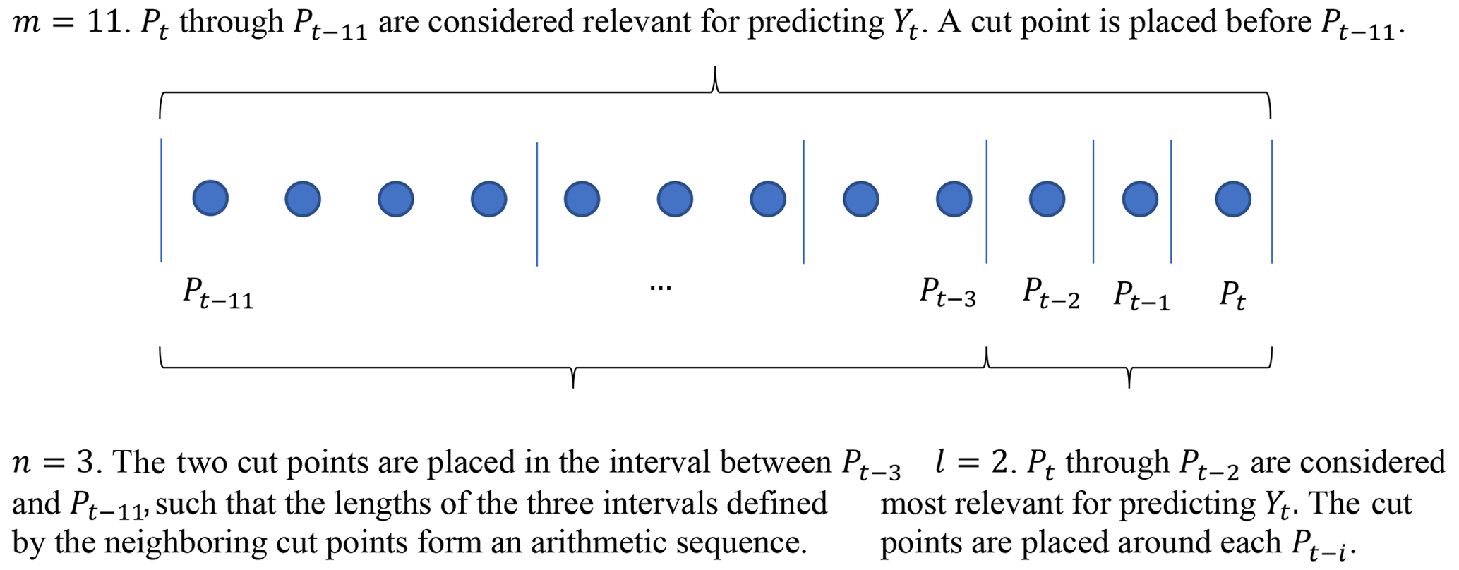
This study proposes a simple method to systematically select cut points along the time axis which form a series of intervals for defining (a,b) pairs. As shown in Fig. 2, the selection of cut points is controlled by three hyperparameters, m, l, and n. (1) For m, a cut point is placed between time steps t−m and , such that the rainfall data recorded prior to time step t−m are considered irrelevant for predicting Yt. (2) For l, the rainfall data recorded between time steps t−l and t−0 are considered to be most relevant for predicting Yt, so that cut points are placed around each time step within this interval. (3) For n, n−1 cut points are placed between time steps and t−m, such that the neighboring cut points correspond to n intervals whose lengths roughly form an arithmetic sequence. After the (a,b) pairs have been defined, a rainfall depth feature is then created for every interval formed by two neighboring cut points.
Representing a rainfall time series using a set of can reduce the dimensionality of data at the cost of losing information regarding the temporal distribution of rainfall. In this method, fewer cut points are selected for rainfall in the long-term past (e.g., a few days ago), which is based on the assumption that they are less important for predicting Yt. This is reasonable, considering the relatively fast response time of SuDS (DeBusk et al., 2011). Similarly, some of the environmental variables may be less important for predicting Yt, which can be filtered out during the feature engineering process. In this study, whether or not to include Ei is controlled by a Boolean variable, and k such variables are used.
In this study, the optimal values of the feature engineering hyperparameters, m, l, n, and the k Boolean variables, are determined using resampling and Bayesian optimization methods as described below.
2.1.3 XGBoost algorithm
This study adopts the gradient-boosted trees algorithm (Friedman, 2001) to train ML models. In particular, the XGBoost (Chen and He, 2020) software library is used. XGBoost is selected for its improved regularization methods, high computational efficiency, and ability to achieve state-of-the-art results on various ML tasks (Nielsen, 2016; Chen and He, 2020; Chen and Guestrin, 2016). A detailed introduction to XGBoost can be found in Chen and Guestrin (2016) and Mitchell and Frank (2017).
A gradient-boosted trees model G is an ensemble of decision trees, in which , the prediction for an input sample xi, is the sum of the predictions of individual trees (Chen and Guestrin, 2016), which is given as follows:
where fk is a decision tree that maps input samples to the values stored at the tree leaves, K is the number of decision trees (also known as the number of boosting iterations), and ℱ is the functional space of all possible regression trees. For a given data set, the structure of the trees, including the splitting criteria and the values stored at the leaves, is learned automatically using XGBoost.
There are a number of hyperparameters used in XGBoost for controlling model structure and the learning behaviors during training, e.g., the number of boosting iterations and maximum tree depth. A complete list of the XGBoost hyperparameters can be found in the software documentation (Chen and He, 2020). In this study, the XGBoost hyperparameters are optimized together with feature engineering hyperparameters using resampling and the Bayesian optimization methods as described below.
2.1.4 Resampling methods and Bayesian optimization for training and testing machine learning models
In this study, the effectiveness of the feature engineering and XGBoost algorithm are evaluated on different data sets of observed (xt,yt) samples collected at different SuDS sites. For each data set, the evaluation is performed by randomly splitting the data set into a series of training and test subsets. For each such split, during the hyperparameter optimization phase, the training set is further split into a series of smaller training and validation data sets. Then, multiple models with different feature engineering and XGBoost hyperparameters are trained on the smaller training data sets, and the quality of a set of hyperparameters is measured by the prediction accuracy of the resulting model on the validation data sets, and the optimal hyperparameters are then identified. During the model evaluation phase, the optimal hyperparameters are then used to fit a model on the training data set (which includes both the smaller training and validation data sets), and the resulting model is evaluated using the test data set. Apparently, the assessment results are affected by how the data set is split; thus, the hyperparameter optimization and model evaluation processes are repeated for various splits in this study for some numerical experiments. More information on resampling methods can be found in Kuhn and Johnson (2013) and Hastie et al. (2009).
During the hyperparameter optimization phase, the candidate hyperparameters to be assessed are proposed by Bayesian optimization methods, which are sample-efficient algorithms for solving black box optimization problems (Shahriari et al., 2016). Bayesian optimization methods are commonly used in ML for hyperparameter optimization (Snoek et al., 2012). The decision variables in the optimization problems are the hyperparameters, and the quantity to be optimized is the prediction accuracy on the validation data sets. An introduction to Bayesian optimization can be found in Frazier (2018).
2.2 Interpreting model structures and inferring hydrological processes learned by machine learning models
2.2.1 Interpreting the basis of each prediction
Understanding why a specific prediction is made by an ML model can be useful for understanding the relationships between various variables captured by the model. In this study, XGBoost uses decision trees as its base learner. Although each decision tree can be considered as a transparent ML model (as the rules used for making predictions can be understood easily by humans), it can be challenging to directly interpret the prediction generation process of an XGBoost model as many trees can be used in it. Therefore, post hoc explainability techniques, such as the gain, cover, and frequency metrics, are commonly used for understanding the structure of XGBoost models.
The gain of a feature is its relative contribution to the model as measured by the total gain of the feature's splits. It can be roughly regarded as a feature's contribution to prediction accuracy improvement (Chen and He, 2020). The cover of a feature is the relative number of training samples related to the feature's splits (Chen and He, 2020). The frequency of a feature is the relative number of times that this feature has been used in tree splits (Chen and He, 2020). The three metrics are global feature importance measures, as they reflect the overall contribution of a feature to an XGBoost model for making various predictions (Guidotti et al., 2019; Ahmad et al., 2018). However, these metrics can be irrelevant for understanding the basis of a specific prediction, which is a task that requires local explanation methods.
This study adopts a local feature attribution method to quantify the contribution of each feature to the prediction made for a specific input sample (Janzing et al., 2019). The SHAP method proposed by Lundberg and Lee (2017) is used in this study. The SHAP value of a feature for a specific input sample can be considered as being the marginal contribution of this feature to the predicted value compared to the mean predictions for all samples. SHAP values satisfy a series of desired properties. For instance, the sum of the SHAP value assigned to each feature equals the difference between the predicted value and the mean prediction for all samples, and the features that do not change the expected prediction are assigned with a SHAP value of 0 (Lundberg et al., 2020). The SHAP values can be computed using the following steps.
Let the real-valued function f of the N-dimensional random variable X be the ML model to be explained, and let be an observed sample of X. ∅i, the SHAP value of xi, is computed as follows:
where, R is a random permutation of the N features, ℛ is the space of all feature permutations, SR is the set of features that are located before feature i in permutation R, and is a set function that maps every subset of the N features (i.e., each member of the power set 𝒫 of all N features) to a real number, and v is known as the value function.
Therefore, ∅i can be interpreted as the expected marginal contribution to v of feature i (i.e., in a random permutation of the N features. Equation (6) is developed based on the Shapley value used in game theory, more information on which can be found in Shapley (1953) and Osborne and Rubinstein (1994).
In the SHAP method, v is the expected prediction of f when some features are missing. v may be defined in various ways. Lundberg and Lee (2017) define v using the observational conditional expectation, which is the expected value of f(X) when the feature values of X for a set of features S are known, as in the following:
Janzing et al. (2019) and Lundberg et al. (2020) defined v using the interventional conditional expectation, as in the following:
where do(S) represents an intervention that sets the feature values of X in S to xS. The SHAP values derived using Eqs. (7) and (8) are respectively termed observational SHAP values and interventional SHAP values. The observational SHAP value of xi generally measures the value of knowing xi to predict the outcome, and the interventional SHAP value of xi corresponds to the expected changes in the model prediction when the feature Xi is set to the xi.
Chen et al. (2020) suggested that both observational and interventional SHAP values are useful. They claimed that the observational SHAP values are true to the data because they are effective in identifying the true correlations between the features and the outcome of interest, whereas the interventional SHAP values are true to the model because they do not credit the features that are unused by the model. The observational SHAP values are used in most places of this paper as they are less computationally expensive than the interventional SHAP values. The TreeSHAP methods proposed in Lundberg et al. (2020) are used in this study to compute both SHAP values.
For a given input sample xt, the SHAP value assigned to a rainfall depth feature can be further distributed among the rainfall recorded at each time step between time steps t−a and t−b. The SHAP value can be assigned to the rainfall recorded at time step t−k proportional to its depth pt−k, where . Thus, τk(xt), the SHAP value assigned to pt−k, if the rainfall depth recorded between time steps t−a and t−b (denoted by ) is not 0, can be computed using the following:
The processes for quantifying the contribution of each feature of an input sample xt to model prediction and distributing the contributions to the rainfall of each time step are illustrated in Fig. 3a.

Figure 3(a) Illustration of the processes for quantifying the contribution of each feature of an input sample xt and distributing the contribution to the rainfall of each time step. (b) Examples of inferring the hydrological processes being modeled based on the basis of each prediction. (c) Examples of comparing the inferred hydrological processes to the expected patterns of the processes derived from domain-specific knowledge of the system being modeled.
2.2.2 Inferring hydrological processes from machine learning modeling results
The process of inferring the hydrological processes being modeled involves mapping from the explanations on the model structure to some imaginary catchments that are likely to possess the characteristics that are consistent with the explanations. For instance, if the explanations indicate that the discharge predictions are strongly controlled by the rainfall in the long-term past, then the processes being modeled are likely to correspond to the processes of catchments with long-term memory effects. However, the mapping processes are inherently subjective and incomplete, and discussions of these characteristics are presented in Sect. 3.6. This section introduces the methods to map the explanations to imaginary catchments, and more discussions on the limitations are given when the case study results are presented.
In this study, for each xt, τk(xt) is computed for pt−k of each time step (Eq. 9). These τk(xt) values quantitatively describe the associations between rainfall and the hydrological response across various time steps, which is useful for inferring the catchment's hydrological processes. For instance, if the predictions are found to be mostly controlled by recent rainfall, then the processes being modeled can correspond to that from a small catchment with a fast response to rainfall. The τk(xt) values can be useful for hydrograph separation. That is, a predicted hydrograph can be decomposed to sub-hydrographs associated with rainfall that occurred in different periods based on their contribution to the predicted discharge, which is different from the current practices that mostly decompose a hydrograph based on the origin of the runoff, such as baseflow and overland flow (Pelletier and Andréassian, 2020). The implications of using this method are discussed in Sect. 3.2.
The SHAP values of multiple samples can be analyzed collectively to obtain a global understanding of the model structure and the system being modeled (Lundberg et al., 2020). This study, thus, computes the expected τk(xt) values for multiple xt in a set S, when k is fixed, to understand the average association between pt−k and f(xt) using the following:
where |S| is the number of elements of S. When S contains all the xt samples, the expectation then approximately describes the overall association between pt−k and f(xt) learned by the model.
SHAP values can be negative, which will result in negative τk(xt) values. To avoid canceling out positive and negative τk(xt) values when computing the expectations, the absolute value of τk(xt) may be used. The quantity of |τk(xt)| can be interpreted as being the importance of pt−k for computing f(xt). The expected value of |τk(xt)| for the xt samples in a set S can be computed using the following:
Similarly, for a given xt, the contribution of rainfall recorded between time steps t−a and t−b, Ta, b(xt), can be simply computed as follows:
Figure 3b gives two examples of inferring hydrological processes from ML modeling results.
2.2.3 Assessing the physical realism of the inferred processes using knowledge
The inferred hydrological processes may be tested in terms of their physical realism. The premise of this test is that if an ML model can provide physically plausible explanations to the processes it models, then its predictions can generally be considered more trustworthy. That is, this test concerns whether the right predictions are made for the right reasons (Kirchner, 2006). The justification of this method is examined in Sect. 3.6.
In the proposed assessment method, the inferred hydrological processes are compared to the hydrological processes that would be expected based on the domain-specific knowledge of the system being modeled. In other words, whether the inferred hydrological processes that are physically plausible are evaluated. In an assessment, the qualitative or quantitative descriptions of the inferred processes and that derived from domain-specific knowledge are used in the comparison. For instance, a small urban catchment is modeled, and it is expected to have a fast response to rainfall. If the inferred hydrological processes correspond to that from a catchment with a long-term memory effect, then the ML model can be considered unreliable. Generally, three possible outcomes are expected in such an assessment.
-
Consistent. These are cases when the inferred hydrological processes are physically plausible according to the domain-specific knowledge of the system being modeled. The term consistent is used, rather than the terms “correct” or “valid”, to reflect that the assessment process involves a comparison to some basis derived from our knowledge of the system being modeled, which might be subjective and incomplete. The term is used following Yang and Chui (2021).
-
Inconsistent. These are cases when the inferred hydrological processes are physically implausible according to the domain-specific knowledge of the system being modeled.
-
Insufficient evidence to draw conclusions. These are cases when definitive conclusions cannot be drawn, which may be caused by the fact that the requirements for the inferred processes to be considered consistent are too specific or too general. For example, assume that the inferred hydrological processes indicate that the catchment has a small surface area (i.e., a qualitative description), and the time of concentration of the catchment being modeled is known from previous studies and is used as the assessment criterion (i.e., a quantitative description). In this context, it is impossible to determine the consistency between the two descriptions unless more evidence regarding the conversion between catchment scale and time of concentration is collected. The inability to draw a definitive conclusion can also be caused by the lack of knowledge of the processes being modeled. For instance, it is difficult to identify the expected hydrological behaviors for ungauged natural catchments.
Figure 3c illustrates the processes for assessing the physical realism of the inferred hydrological processes.
2.3 Case studies
2.3.1 Study sites
There are two SuDS sites with different drainage areas, SuDS practice types, and data availabilities examined in this study. Study site 1 is located on Washington Street, Geauga County, Ohio, USA (hereinafter referred to as WS). Multiple types of SuDS were built in WS to treat stormwater runoff generated by a nearby commercial building and parking lot, as shown in Fig. 4a (Darner et al., 2015). Runoff from approximately half of the commercial building roof (i.e., an impervious area of 316 m2) drain into a rain garden with a surface area of 37 m2. The 762 m2 parking lot was constructed using porous pavements to allow infiltration.

Figure 4(a) Layout of the SuDS and monitoring network on the Washington Street site (WS), Geauga County, Ohio, USA. This figure is adapted from Darner et al. (2015). (b) Map of the Shayler Crossing Watershed (SHC). The subcatchment boundaries and drainage system shown on the map are defined by Lee et al. (2018a).
Study site 2 is the Shayler Crossing Watershed (SHC) in Clermont County, Ohio, USA, as shown in Fig. 4b. SHC is a sub-watershed of the East Fork Little Miami River watershed. The drainage area of SHC is approximately 0.92 km2 (Hoghooghi et al., 2018), and the land use type is primarily residential. The drainage system of SHC consists of conduits, channels, detention ponds, dry ponds, and wet ponds (Lee et al., 2018a). In SHC, stormwater runoff generated by indirectly connected impervious areas (e.g., sidewalks) is treated by the nearby pervious areas, which are termed buffering pervious areas and have similar functions to grass filter strips (Lee et al., 2018b). SHC represents a typical residential area in the USA and is thus selected to test the applicability of the proposed ML methods in modeling small urban catchments.
In WS, a 10 min resolution rainfall discharge time series is available from on-site monitoring between 2009 and 2013. The outflow from WS was collected and measured by three flumes. Flumes 1, 2, and 3, respectively, collect the surface runoff from the parking lot, overflow from the surface layer of the rain garden, and underdrain flows from the parking lot. The on-site monitoring was conducted by the United States Geological Survey (USGS), and more details of the monitoring work can be found in Darner and Dumouchelle (2011) and Darner et al. (2015). In SHC, 10 min resolution rainfall time series from 2009–2010 is available, in addition to a 10 min resolution discharge time series measured at the outlet between July and August 2009 by the USA Environmental Protection Agency. The data set used in this study is the same as in Lee et al. (2018a, b), in which more details on the data set can be found.
It can be challenging to set up process-based models for both sites. In WS, the physical properties and exact design of the different drainage system elements are not precisely known (Darner et al., 2015). For instance, the rain garden is not isolated from the gravel storage layer of the porous pavements; however, the exact flow conditions in the storage layer are unknown. In SHC, the main challenge lies in the heavy workload and uncertainties in estimating the model parameters that characterize the complex drainage system. For example, to accurately represent the drainage processes, SHC should be divided into multiple subcatchments connected by a drainage network, and each subcatchment should be further subdivided into multiple subareas, such as directly and indirectly connected impervious subareas (Lee et al., 2018a). The task of the sub-area division, however, requires substantial effort, considering the relatively large number of subcatchments that are involved.
2.3.2 Numerical experiments
Rainfall–runoff models are built for both SHC and WS using ML methods. In WS, the output variable is the flow rate of the total runoff collected by the three flumes recorded at regular 10 min intervals during the warm season (i.e., April to October; Darner et al., 2015). The input variables include the 10 min resolution rainfall time series recorded prior to runoff, the month in which the runoff occurs (optional), and the accumulative rainfall depth recorded since the beginning of monitoring (optional). The optional features are considered to account for the possible time-varying performance of the SuDS during its service life (Yong et al., 2013) and the potential seasonality of the SuDS hydrological properties (Muthanna et al., 2008). Whether the two sets of optional features should be included is controlled by two binary feature engineering hyperparameters, and the other three feature engineering hyperparameters are m, l, and n, as described in Sect. 2.1.2. The ranges of the hyperparameter values are listed in Table 1, and their optimal values are determined using Bayesian optimization methods. The rainfall discharge data collected between 2010 and 2013 by USGS are used in this study. A total of 142 independent rainfall events are identified using a 24 h dry spell threshold (Guo and Senior, 2006). A nested cross-validation (CV) resampling procedure is implemented in which a five-fold CV is used for both the inner and outer CV iterations. The folds are created using a rainfall-event-grouped stratified sampling method (Zeng and Martinez, 2000), i.e., data associated with the same rainfall event are grouped into the same fold, and the peak discharge of the rainfall events in each fold roughly follows the same distribution. This is to prevent data leakage and ensure that the data in each fold are representative (Kuhn and Johnson, 2013). In general, each outer CV iteration can be considered as being an experiment to assess the effectiveness of an ML method using a specific split of the data set, and its associated inner CV iterations are considered as being procedures to derive the model to be evaluated on the test data set.
Table 1Hyperparameter values considered for the two study sites.
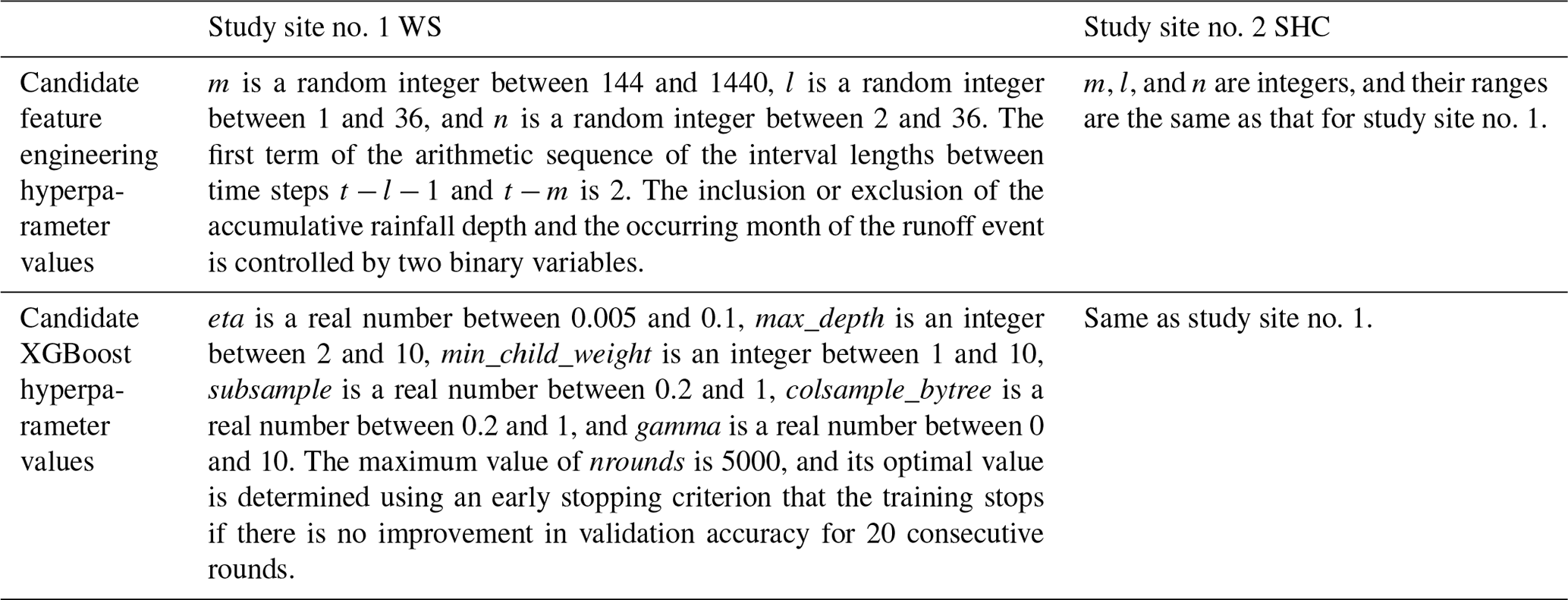
In SHC, the output variable is the watershed outlet discharge measured at 10 min intervals, and the input variable is the rainfall time series recorded before the discharge measurement. Only 2 months of runoff data are available in this study. The nested CV procedure is not used due to the small data set size; instead, the data set is split into training, validation, and test data sets that each contains at least one large runoff event. The Bayesian optimization methods are then used to identify the optimal hyperparameters (as shown in Table 1) that minimize the prediction error on the validation data set when the model is trained on the training data set. The training and validation data sets are then combined, and the ML methods with the optimal hyperparameters are applied. The resulting models are then tested on the test data set.
For each site, the resampling and hyperparameter optimization methods are also applied to train linear regression models, which are used as a baseline for evaluating XGBoost models. The only difference in the training processes between the two model types is that only the feature engineering hyperparameters are used when fitting linear regression models to the data. For SHC, the process-based model developed by Lee et al. (2018a) is also compared with the ML models built in this study. Their model is built using SWMM software, in which SHC is divided into 191 subcatchments, and the drainage processes in each subcatchment are characterized using various parameters. The prediction accuracies of different types of models are then compared for each site.
The proposed method is then applied to explain the basis of each prediction for the two sites, i.e., for each discharge prediction, the contribution of rainfall of each time step (i.e., τk(xt)) is computed. Both the observational and interventional SHAP values are used in the derivation, which results in two versions of the τk(xt) values. The following experiments on inferring hydrological processes from ML modeling results are conducted based on the τk(xt) values.
-
The predicted hydrographs are decomposed into multiple hydrographs associated with the rainfall recorded between the past 0–1, 1–2 h, and so on using Eq. (12). Whether the hydrograph separation method can generate physically plausible results is examined using a few simple hydrological principles, which include the following: (a) rainfall have positive contributions to runoff, and (b) runoff in small urban catchments are mostly contributed by rainfall that occurred in the recent past.
-
The overall importance of rainfall of each time step to discharge prediction (Eq. 11) is computed for each site using all the samples. These importance scores are then used to infer the hydrological processes of the system being modeled. The physical realism of the inferred processes is evaluated using principles derived from hydrological knowledge of the system being modeled, which includes the idea that (a) smaller catchments commonly have faster responses to rainfall compared to larger catchments and (b) the importance scores of rainfall change smoothly across time steps. Principle (b) is derived from hydrological knowledge that rainfall of similar magnitudes in adjacent time steps are expected to have similar impacts on the runoff generation processes.
-
This experiment aims to investigate whether different ML explanation methods lead to similar inferred hydrological processes. The gain, cover, and frequency metrics are computed for each XGBoost model of WS. These scores are then distributed among rainfall of each time step proportionally to its associated rainfall depth of all the samples, and the resulting quantities are compared to the normalized importance scores derived in experiment no. 2. The SHAP-related importance scores are normalized such that the resulting scores associated with all predictors sum to 1.
-
This experiment aims to investigate whether more accurate models are more likely to provide physically plausible explanations to the physical processes being modeled. The XGBoost models trained using 10 %, 20 %, 40 %, and 60 % of the observed samples of WS are evaluated in terms of their prediction accuracy and ability to provide consistent explanations to the modeled processes. The models' optimal hyperparameters are estimated using a resampling method (i.e., a training–validation split) and Bayesian optimization methods. The test data set used in prediction accuracy estimation contains 40 % of the samples and is the same for all models (that are trained on data sets of various sizes). The remaining 60 % of the samples are then used for creating training data sets that contain 10 %, 20 %, 40 %, and 60 % of the samples. Note that the training data set that contains 60 % of the samples is created using all the remaining samples (that are not contained in the test data set). For each training data set, a further training–validation split is defined, and 10 models are then trained by repeatedly applying the Bayesian optimization methods (which are stochastic). For each sample size, the training data set creation and training–validation splitting procedures are repeated 10 times and each such procedure produces 10 models (by applying Bayesian optimization methods repeatedly). That is, 100 versions of models are derived for each sample size. The importance score of rainfall of each time step is then derived following the methods in experiment no. 2, which is then used to infer the hydrological processes being modeled. The consistency of the inferred processes is then evaluated based on whether the importance scores of rainfall change smoothly across time steps using the test data set, where a threshold of L/s is used to account for numerical error.
3.1 Prediction accuracy of machine learning models
The prediction accuracies of the various WS and SHC models are compared in Fig. 5. The root mean square error (RMSE), coefficient of determination (R2), and Nash–Sutcliffe coefficient of efficiency (NSE; Nash and Sutcliffe, 1970) of the predictions on the test data sets are compared, except for the SWMM model developed by Lee et al. (2018a), which was tested on a part of its training data set due to small data set size. The prediction accuracies of the XGBoost models, i.e., NSE>0.7 and R2>0.7, can be considered satisfactory, considering that they were relatively easy to set up and that it was impossible or very difficult to build process-based models for either site. The XGBoost models for both sites consistently outperform the linear regression (LM) models, suggesting that more sophisticated ML algorithms, such as XGBoost, are able to better capture the complex rainfall–runoff correlations than simple LM methods. The SHC XGBoost models have comparable prediction accuracies to SWMM, although the former were built with considerably less effort. Thus, in future SuDS studies, it can be useful to quickly train some ML models based on available data and use them as a reference to evaluate the prediction accuracies of process-based models. The proposed ML model training methods can be potentially extended to study other small-scale urban catchments that have similar configurations to SHC.
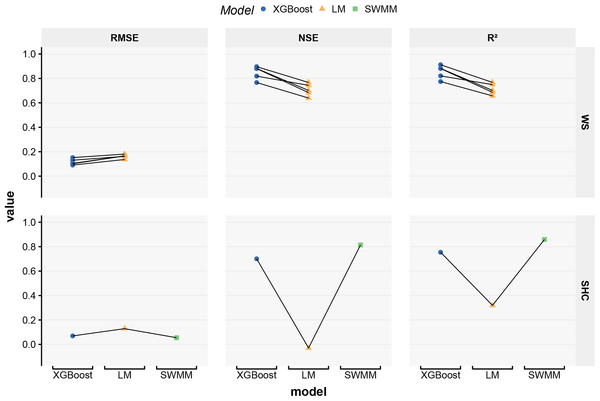
Figure 5Prediction accuracies of the various models built for the Washington Street SuDS site (WS) and Shayler Crossing Watershed (SHC). The prediction accuracies are evaluated in terms of the root mean square error (RMSE), coefficient of determination (R2), and Nash–Sutcliffe coefficient of efficiency (NSE). The RMSE units are liters per second (hereafter L/s) for WS and cubic meters per second (hereafter m3/s) for SHC. Each data point in the figure shows the prediction accuracy evaluated using a specific split of the data set. The prediction accuracies derived using the same test data set are connected by lines. The SWMM model for SHC was built by Lee et al. (2018a).
Each data point in Fig. 5 shows the results obtained for a specific split of a data set (i.e., the division of data into training, validation, and test data sets), and the points that correspond to the same split are connected by lines. The prediction accuracies of XGBoost and LM models varied considerably for different splits of a data set. The variations indicate that the sample distributions in the different versions of training and test data sets appreciably differ, even though a stratified sampling method was used to balance the sample distribution in the different folds. The imbalanced sample distribution is associated with the limited number of samples used for the model training and evaluation, which implies that the 4 years of rainfall–runoff data of WS still contained an insufficient number of samples for the ML methods examined in this study. For instance, only a few high-flow events were observed each year in WS, which may be insufficient for training ML models that provide accurate high-flow predictions. Even fewer samples were available for training and testing the SHC models; thus, the uncertainties of the prediction accuracies may be even larger.
3.2 Physical realism of the decomposed hydrographs
The results obtained for numerical experiment no. 1 are presented in this section. As an example, Fig. 6 shows the predicted decomposed hydrographs of WS associated with rainfall of different periods for a large, medium, and small runoff event. As shown in Fig. 6, runoff is mostly contributed by the rainfall that occurred within the past 1 h, regardless of the runoff event magnitude, especially for the peak discharge. These patterns are generally expected from small catchments, where runoff are mostly contributed by recent rainfall. As WS is a small-scale catchment, the inferred fast runoff responses are consistent with our hydrological knowledge.

Figure 6(a) Rainfall time series and (b) decomposed hydrographs of a large, medium, and small runoff event from the Washington Street SuDS site (WS). The model used to derive the hydrographs was obtained in the outer cross-validation iteration 1. Observational SHAP values were used in the computation.
Although it is not exactly clear how to quantitatively assess the physical realism of the contribution values assigned to rainfall of each hour, they express some patterns that are obviously inconsistent with our hydrological knowledge. First, Fig. 6 shows that rainfall can have negative contributions to runoff, which are physically impossible. Although rainfall is the only forcing variable that is used by the model, the negative contributions may also be explained by the other implicit variables that can be predicted by rainfall, e.g., evapotranspiration is correlated with rainfall and can cause water losses from the catchment. However, it is nontrivial to exclude the contributions of the implicit variables such that rainfall's contributions to runoff are strictly nonnegative. Second, there is a constant bias term in the decomposed hydrographs that are independent of the rainfall. This term is the average prediction for all samples and accounts for the differences between the predicted values and the contributions assigned to all variables in the SHAP method. However, this constant term does not clearly correspond to any processes in hydrology. Additionally, a model might use features that are not derived from rainfall (e.g., the age of the SuDS practice) as a predictor, which will also be assigned with contributions to runoff when the SHAP method is used to examine the basis of predictions. However, it is unclear how to use these contributions in hydrograph separation.
The results of this experiment show that the inferred hydrological processes can be only partially consistent with the knowledge of the system being modeled. Some ML explanation methods, such as SHAP, can generate explanations that are inherently inconsistent with hydrological principles, such as the rainfall's negative contributions to runoff and the constant contributions to runoff that are not associated with any variable. Nevertheless, it would be meaningful to compare the decomposed hydrographs to those derived using approaches in process-based modeling and tracer and isotope hydrology to further evaluate the validity of the explanations derived using ML methods.
3.3 Physical realism of the importance of rainfall of different time steps to discharge prediction
The results of numerical experiment no. 2 are shown in Fig. 7. In both WS and SHC, rainfall recorded prior to 100 time steps in the past (i.e., 16.7 h) have almost no impact on discharge prediction, which is reasonable considering their small catchment sizes. The rainfall that occurred in 1 and 4 time steps (i.e., 10 and 40 min) in the past are found to have the highest impact on discharge prediction for WS and SHC, respectively. This pattern is expected as SHC is considerably (which is around 800 times) larger than WS, and thereby, the time required for stormwater to travel through the catchment is also longer in SHC. Although the exact response time of both catchments is unknown, it is possible to use the knowledge regarding the relations between the response time of the two catchments to conduct an assessment. Utilizing relational patterns in assessing the consistency of multiple entities has been demonstrated in Yang and Chui (2021).
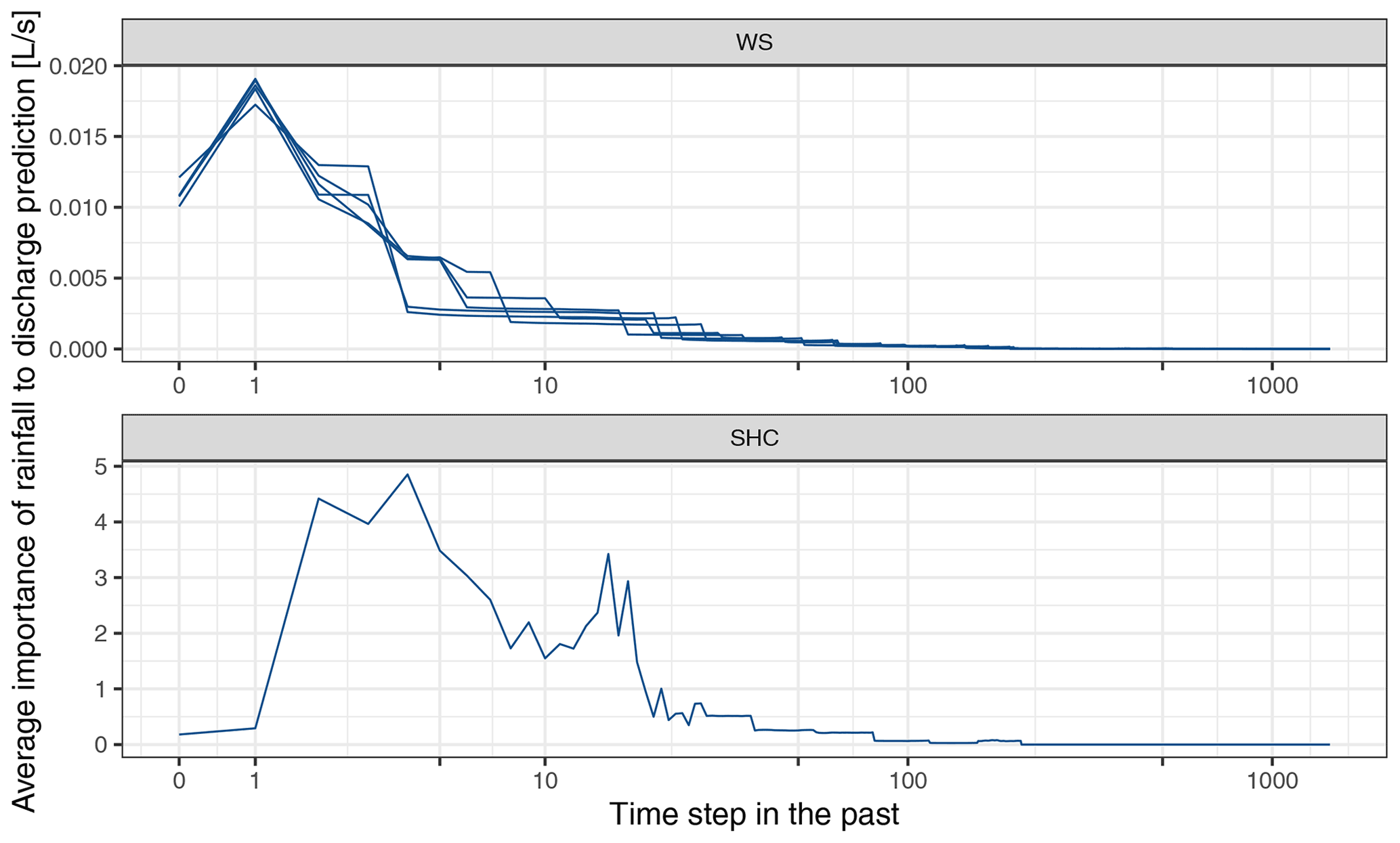
Figure 7Average importance of the rainfall at different time steps in the past for discharge predictions in the XGBoost models of the Washington Street SuDS site (WS) and the Shayler Crossing Watershed (SHC). Each line corresponds to an XGBoost model trained on a specific training data set. Each time step is 10 min. The x axis is on a pseudo-logarithmic scale. Observational SHAP values were used in the computation.
It is also worth noting that the importance scores assigned to rainfall fluctuate across time steps for SHC, which indicates that the models find that the rainfall in some specific time steps is more important for discharge prediction when compared to the others, which is inconsistent with our hydrological knowledge. In WS, these inconsistent patterns are not observed where the importance scores of rainfall generally change monotonically from the past 1 time step to the current time step and the time steps in the more distant past. The inconsistent patterns might be caused by insufficient data used in model training and evaluation, which is discussed further in Sect. 3.5.
In WS, the rainfall of a specific time step can be assigned with notably different importance scores when the models trained using different training data sets are used, which is an indication of considerably different model structures. The structural differences in ML models are also reported in Schmidt et al. (2020), where the existence of multiple possible model structures is referred to as equifinality (Beven and Freer, 2001). The different importance scores will naturally result in different explanations of the processes being modeled, and apparently, these explanations cannot be simultaneously close to reality (Bouaziz et al., 2021). However, in this case, it is not possible to quantitatively assess the explanations provided by different models due to the lack of knowledge. Experiment no. 4 investigate whether models with higher prediction accuracies can generate more trustworthy explanations to the process being modeled, and the results are presented in Sect. 3.5.
3.4 Comparison of multiple methods for explaining machine learning modeling results
The results of experiment no. 3 are shown in Fig. 8, where various feature importance scores of rainfall of different time steps are compared. All the importance scores derived using different methods suggest that the rainfall of more recent time steps have a higher impact on discharge prediction. However, different methods can derive considerably different importance scores for the rainfall of a specific time step, and the relations between the importance scores assigned to the rainfall of different time steps also vary among different methods. Some methods, such as interventional SHAP and frequency, are more sensitive to model structural differences than others. The differences in various importance scores indicate that the selection of the explanation method is another source of uncertainty in inferring the processes being modeled.
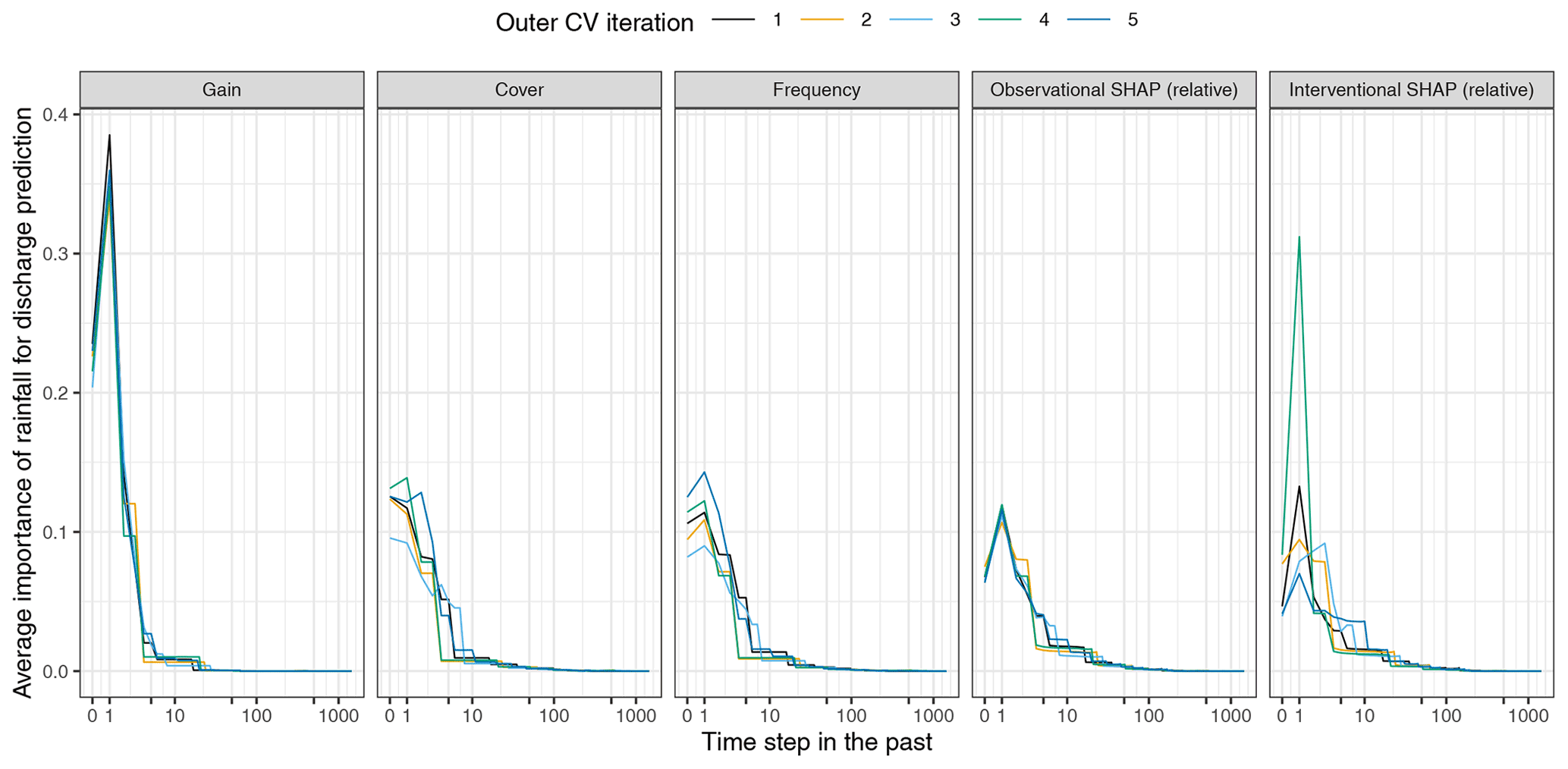
Figure 8The importance of rainfall from each time step for making discharge predictions assessed by different feature importance measures in the Washington Street SuDS site (WS) XGBoost models. Each line shows the results of model trained during an outer cross-validation (CV) iteration. The x axis is on a pseudo-logarithmic scale. For interventional SHAP, all the training samples are used as background data set.
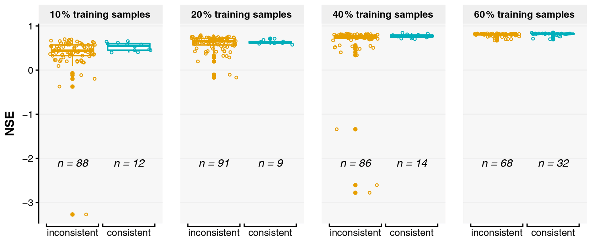
Figure 9Box plot of the prediction accuracy, as measured by the Nash–Sutcliffe coefficient of efficiency (NSE), of the Washington Street SuDS site (WS) XGBoost models when samples of different sizes are used in model training. For each sample size, the models that offer consistent or inconsistent explanations are grouped together, and the numbers of consistent and inconsistent models (the n values) are shown. Observational SHAP values were used in the computation.
The importance scores derived from the observational and interventional SHAP values varied significantly due to the different methods used for computing the expected prediction, i.e., Eqs. (7) to (8). It is, however, currently unclear how to evaluate an explanation method's effectiveness in inferring the processes being modeled. Nevertheless, it is recommended that future studies always report the configurations of the explanation methods being used and evaluate the uncertainties associated with the explanation method selection.
3.5 Correlation between the physical realism of inferred processes and model prediction accuracy
The results of experiment no. 4 are discussed in this section. As shown in Fig. 9, a models' prediction accuracy, as measured by NSE, generally increases as more samples are used to train the model, despite its large uncertainties associated with the random sampling of the data set. However, the number of models that correspond to consistent explanations (i.e., the single-peaked patterns of rainfall importance scores), also shown by the numbers in Fig. 9, did not increase as more samples are used in training. In fact, consistent results are not often observed for all training sample sizes. These results suggest that more accurate models do not necessarily offer more physically realistic explanations to the processes being modeled, and using more data samples in model training does not guarantee more physically realistic explanations. For the models trained with the same amount of data, selecting a more accurate model does not guarantee that the inferences made based on the selected model are more consistent with our knowledge. However, it is also possible that our knowledge used in the assessment is biased, and the test data set may not represent the true data distribution that would be observed on an infinite timescale.
Ilyas et al. (2019) argued that ML models can make predictions based on features that humans cannot comprehend. The implication of this argument is that ML models can make the right predictions for the wrong reasons (Ross et al., 2017) or reasons that are inconsistent with our knowledge, and therefore, the prediction accuracy of a model is not a trustworthy measurement of the physical realism of the explanations it provides. Regularizing ML models using physical principles, as suggested in Nearing et al. (2021), can potentially increase the physical realism of the explanations and the inferred physical processes.
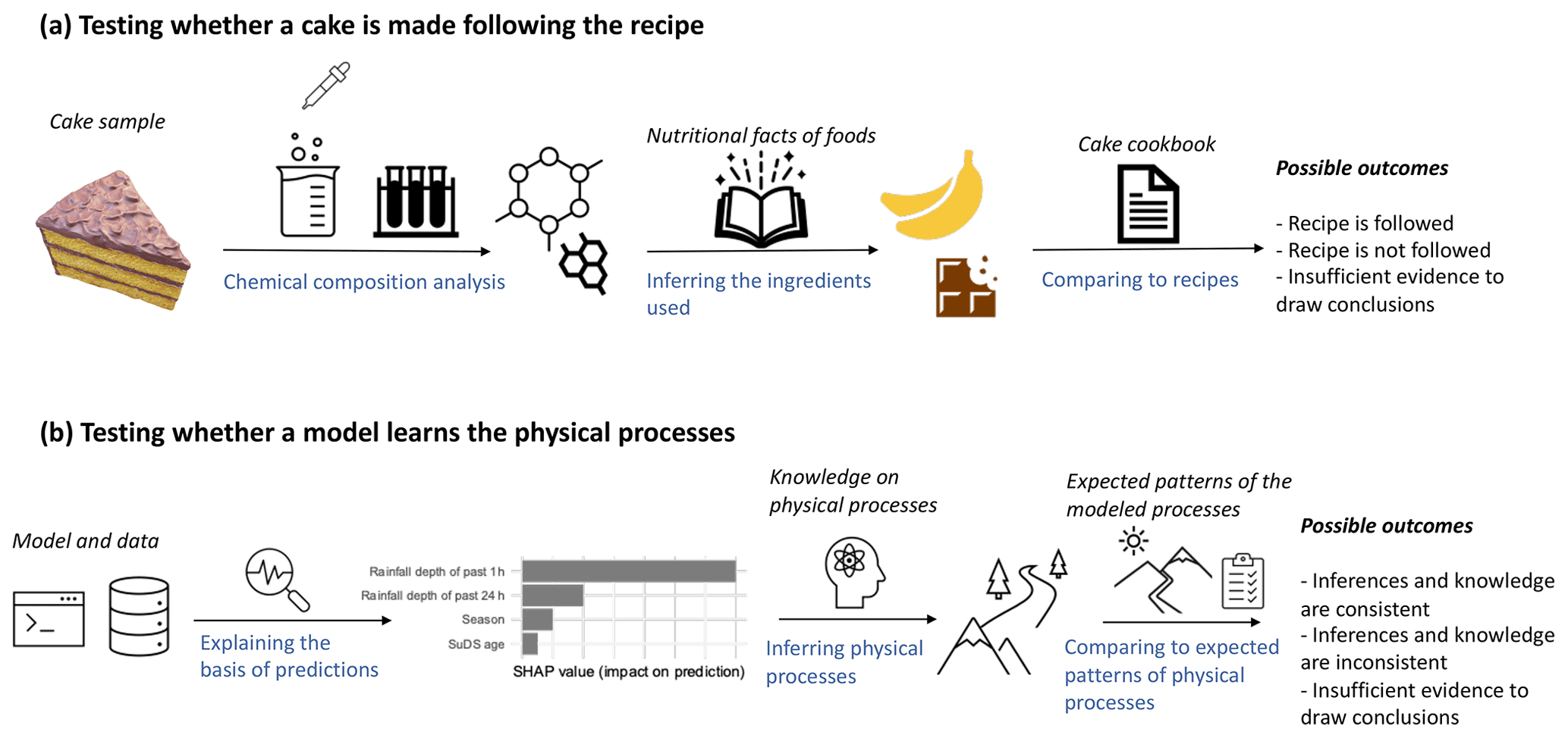
Figure 10Illustration of the processes of (a) testing whether a cake is made following the desired recipe and (b) testing whether a model captures the physical processes of the system being modeled.
3.6 Inferring hydrological processes using machine learning methods and analyzing ingredients of cake samples
This section uses a metaphor to explain the processes of inferring hydrological processes using ML methods, as shown in Fig. 10. An ML model is similar to a cake (baked by others) in that they both are consumed by humans, and the exact mechanisms that generate the outcomes (i.e., the predictions or the tastes) are often unknown due to complexity. Here, the mechanisms refer to the numerical operations that generate the predictions or the ingredients and procedures that give the flavor. Normally, the predictions or the tastes are of primary interest. However, it can be useful to inspect the mechanisms that lead to the outcomes such that more confidence regarding future outcomes can be gained, where future outcomes refer to the predictions under new conditions or more cakes acquired through similar means. ML explanation methods and chemical composition analysis methods can provide information regarding the elements that contribute to the prediction or flavor. However, in many cases, such information can only be treated as circumstantial evidence of certain physical principles being learned by a model or the presence of certain ingredients. This is because ML models usually do not have structures that directly resemble the physical processes and chemical composition analysis usually does not directly test the presence of a food ingredient. The raw information is then further processed by referring to domain-specific knowledge, such as hydrological knowledge or the nutritional facts of foods. For instance, a high degree of association between the predicted discharge and recent rainfall is an indication of a catchment's fast runoff response, which is commonly seen in small urban catchments, and a high carotene content may indicate that carrots are used in the cake. The inferred physical processes or ingredients and procedures are then evaluated against what would be expected based on domain-specific knowledge of the system being modeled or baking a specific type of cake. Finally, whether the ML model learns the expected physical processes or whether the cake is baked following the expected recipe is evaluated.
It is important to note that uncertainties are presented in every step of the assessment. First, different ML explanation methods or chemical composition analysis methods can lead to significantly different outcomes, which are used as the basis for inference. An example is provided in Sect. 3.4. Second, the inference process can be biased and subjective due to our incomplete knowledge. For example, a chemical component could correspond to an ingredient that we do not know, and rainfall's negative contribution to runoff could be caused by an unknown stormwater harvesting activity in the catchment. Bias and subjectivity, however, cannot be avoided in an open system, as there may be infinitely many physically plausible explanations to the same outcome (Oreskes et al., 1994). Third, the knowledge applied in the final assessment processes to define assessment criteria can be incomplete.
Are the practices of inferring the physical processes using ML methods any good? This study considers the consistency evaluation results of the inferences as circumstantial evidence to support a model's trustworthiness. Although an ML model does not have to learn the physical principles to make good predictions, we might prefer that the desired principles are captured by the models. This is similar to suggesting that we prefer delicious cakes made with ingredients we considered safe. Models that are associated with inferences that are consistent with our knowledge may be proven to be more reliable under new circumstances, such as extreme event predictions and predictions under data distribution drifts (Lu et al., 2019). More research on testing ML models' reliability is recommended.
It is also important to note that the inferred processes should be interpreted cautiously due to the large uncertainties involved in every step of the assessment. The detailed configurations of the entire inference process should be reported when presenting the inferred processes. In particular, large uncertainty resides in the process of making inferences according to the raw explanations derived from ML explanation methods, as many physical processes can give rise to the same raw explanations. It is, therefore, important to consider a larger search space for drawing inferences, which may be considered as an attempt to mitigate the streetlight effect, i.e., limiting the search space to be only under a streetlight in the dark or a specific set of plausible explanations (Demirdjian et al., 2005).
The following conclusions can be drawn.
-
This study shows that ML methods can be useful for modeling the hydrological responses of SuDS catchments at sub-hourly timescales. In this study, models with high prediction accuracies (NSE >0.7) are obtained for two SuDS catchments of different sizes, SuDS practice types, and data availabilities. ML models can be set up relatively easily, provided that observation data of the variables of interest are available and, thus, are recommended to be used as a reference to evaluate process-based models.
-
The physical processes being modeled can be inferred based on the results of ML explanation methods. However, the inferred processes might be inconsistent with the patterns that would be expected based on the domain-specific knowledge of the system being modeled. An ML model's ability to provide accurate predictions can be uncorrelated with its ability to offer plausible explanations to the physical processes being modeled.
-
This study provides a high-level overview of the processes of inferring the physical processes being modeled using ML explanation methods. It shows that large uncertainties are presented in the processes of explaining model structures using ML explanation methods, making inferences according to the raw explanations, and assessing the physical realism of the inferred physical processes. The inferred hydrological processes normally should only be considered as circumstantial evidence to support a model's trustworthiness due to their indirect connection to the raw explanations. Due to the existence of the large uncertainties in the inference processes, the inferred physical processes should be interpreted cautiously, and more physically plausible explanations that correspond to the same raw explanations can be potentially investigated.
The source code used in this study is available at https://doi.org/10.5281/zenodo.5652719 (stsfk, 2021), which contains functions for data pre-processing, modeling, modeling result analysis, and plotting. The following R packages are used for modeling and analysis in this research: xgboost (Chen and He, 2020), tidymodels (Kuhn and Wickham, 2020), lubridate (Grolemund and Wickham, 2011), RcppRoll (Ushey, 2018), zeallot (Teetor, 2018), mlrMBO (Bischl et al., 2017), and hydroGOF (Zambrano-Bigiarini, 2020). The following Python packages are used: shap (Lundberg and Lee, 2017), NumPy (Harris et al., 2020), and xgboost (Chen and Guestrin, 2016). All the R and Python packages used in this research are freely available online.
The data of the two study sites examined in this study have been obtained from the United States Geological Survey (USGS), Clermont County, Ohio, USA, and the United States Environmental Protection Agency (U.S. EPA). The identification numbers of the USGS monitoring sites for the Washington Street SuDS site (WS) are 412533081221500, 412535081221400, and 412535081221402. The data of the Shayler Crossing Watershed can be downloaded from https://doi.org/10.23719/1378947 (EPA, 2017). The SWMM model used in this research is developed in Lee et al. (2018a).
YY designed the study, acquired the data, wrote the code, conducted the numerical experiments, analyzed the results, and prepared and revised the paper. TFMC contributed to the design of numerical experiments, supervised the study, validated the results, and revised the paper.
The authors declare that they have no conflict of interest.
Publisher's note: Copernicus Publications remains neutral with regard to jurisdictional claims in published maps and institutional affiliations.
The work described in this paper was partly supported by a grant from the Research Grants Council of the Hong Kong Special Administrative Region, China (project no. HKU17255516), and partly supported by the RGC Theme-Based Research Scheme (grant no. T21-711/16-R) funded by the Research Grants Council of the Hong Kong Special Administrative Region, China. We thank Robert Darner, from USGS, Christopher Nietch and Michelle Simon, from U.S. EPA, Joong Gwang Lee, from the Center for Urban Green Infrastructure Engineering, and Bill Mellman, from Clermont County Water Resources, for providing data for this research. We are grateful for the comments from Omar Wani and Hoshin Gupta on evaluating the physical realism of machine learning models in hydrological studies. We also would like to thank Georgia Papacharalampous, Francesco Granata, and one anonymous reviewer, for providing insightful feedback that greatly improved the quality of this paper. Finally, we wish to thank the editor, Roberto Greco, for handling and assessing our paper during the review processes.
This research has been supported by the Research Grants Council of the Hong Kong Special Administrative Region, China (grant nos. HKU17255516 and T21-711/16-R).
This paper was edited by Roberto Greco and reviewed by Georgia Papacharalampous, Francesco Granata, and one anonymous referee.
Ahmad, M. A., Teredesai, A., and Eckert, C.: Interpretable machine learning in healthcare, in: Proceedings – 2018 IEEE International Conference on Healthcare Informatics, ICHI 2018, p. 447, 4 to 7 June 2018, New York City, NY, USA, 2018.
Barredo Arrieta, A., Díaz-Rodríguez, N., Del Ser, J., Bennetot, A., Tabik, S., Barbado, A., Garcia, S., Gil-Lopez, S., Molina, D., Benjamins, R., Chatila, R., and Herrera, F.: Explainable Artificial Intelligence (XAI): Concepts, taxonomies, opportunities and challenges toward responsible AI, Inf. Fusion, 58, 82–115, https://doi.org/10.1016/J.INFFUS.2019.12.012, 2020.
Beven, K. and Freer, J.: Equifinality, data assimilation, and uncertainty estimation in mechanistic modelling of complex environmental systems using the GLUE methodology, J. Hydrol., 249, 11–29, https://doi.org/10.1016/S0022-1694(01)00421-8, 2001.
Bischl, B., Richter, J., Bossek, J., Horn, D., Thomas, J., and Lang, M.: mlrMBO: A Modular Framework for Model-Based Optimization of Expensive Black-Box Functions, arXiv [preprint], arXiv:1703.03373v3, 2017.
Bojanowski, P., Joulin, A., Paz, D. L., and Szlam, A.: Optimizing the latent space of generative networks, in: 35th International Conference on Machine Learning, ICML 2018, vol. 2, 960–972, Stockholm, Sweden, 10 to 15 July 2018, 2018.
Bouaziz, L. J. E., Fenicia, F., Thirel, G., de Boer-Euser, T., Buitink, J., Brauer, C. C., De Niel, J., Dewals, B. J., Drogue, G., Grelier, B., Melsen, L. A., Moustakas, S., Nossent, J., Pereira, F., Sprokkereef, E., Stam, J., Weerts, A. H., Willems, P., Savenije, H. H. G., and Hrachowitz, M.: Behind the scenes of streamflow model performance, Hydrol. Earth Syst. Sci., 25, 1069–1095, https://doi.org/10.5194/hess-25-1069-2021, 2021.
Charlesworth, S. M.: A review of the adaptation and mitigation of global climate change using sustainable drainage in cities, J. Water Clim. Chang., 1, 165–180, https://doi.org/10.2166/wcc.2010.035, 2010.
Chen, H., Janizek, J. D., Lundberg, S., and Lee, S. I.: True to the model or true to the data?, arXiv [preprint], arXiv:1805.11783, 2020.
Chen, T. and Guestrin, C.: XGBoost: A scalable tree boosting system, in: Proceedings of the ACM SIGKDD International Conference on Knowledge Discovery and Data Mining, 13–17 August, 785–794, San Francisco, CA, USA, 2016.
Chen, T. and He, T.: xgboost: eXtreme Gradient Boosting, available at: https://cran.r-project.org/web/packages/xgboost/vignettes/xgboost.pdf, last access: 29 June 2020.
Damodaram, C., Giacomoni, M. H., Prakash Khedun, C., Holmes, H., Ryan, A., Saour, W., and Zechman, E. M.: Simulation of combined best management practices and low impact development for sustainable stormwater management, J. Am. Water Resour. Assoc., 46, 907–918, https://doi.org/10.1111/j.1752-1688.2010.00462.x, 2010.
Darner, R. A. and Dumouchelle, D. H.: Hydraulic Characteristics of Low-Impact Development Practices in Northeastern Ohio, 2008-2010: U.S. Geological Survey Scientific Investigations Report 2011–5165, available at: https://pubs.usgs.gov/sir/2011/5165/ (last access: 7 July 2020), 2011.
Darner, R. A., Shuster, W. D., and Dumouchelle, D. H.: Hydrologic Characteristics of Low-Impact Stormwater Control Measures at Two Sites in Northeastern Ohio, 2008–2013: U.S. Geological Survey Scientific Investigations Report 2015-5030, U.S. Geological Survey, Reston, VA, USA, 2015.
DeBusk, K. M., Hunt, W. F., and Line, D. E.: Bioretention Outflow: Does It Mimic Nonurban Watershed Shallow Interflow?, J. Hydrol. Eng., 16, 274–279, https://doi.org/10.1061/(ASCE)HE.1943-5584.0000315, 2011.
Demirdjian, D., Taycher, L., Shakhnarovich, G., Grauman, K., and Darrell, T.: Avoiding the “streetlight effect”: Tracking by exploring likelihood modes, in: Proceedings of the IEEE International Conference on Computer Vision, vol. I, 357–364, San Diego, CA, USA, 20 to 26 June 2005, 2005.
Eckart, K., McPhee, Z., and Bolisetti, T.: Performance and implementation of low impact development – A review, Sci. Total Environ., 607–608, 413–432, https://doi.org/10.1016/j.scitotenv.2017.06.254, 2017.
Elliott, A. H. and Trowsdale, S. A.: A review of models for low impact urban stormwater drainage, Environ. Model. Softw., 22, 394–405, https://doi.org/10.1016/j.envsoft.2005.12.005, 2007.
EPA: Flow and Rainfall Data used for SHC Headwatershed SWMM Calibration, EPA [data set], https://doi.org/10.23719/1378947, 2017.
Eric, M., Li, J., and Joksimovic, D.: Performance Evaluation of Low Impact Development Practices Using Linear Regression, Br. J. Environ. Clim. Chang., 5, 78–90, https://doi.org/10.9734/bjecc/2015/11578, 2015.
Fassman-Beck, E., Hunt, W., Berghage, R., Carpenter, D., Kurtz, T., Stovin, V., and Wadzuk, B.: Curve number and runoff coefficients for extensive living roofs, J. Hydrol. Eng., 21, 04015073, https://doi.org/10.1061/(ASCE)HE.1943-5584.0001318, 2016.
Fletcher, T. D., Shuster, W., Hunt, W. F., Ashley, R., Butler, D., Arthur, S., Trowsdale, S., Barraud, S., Semadeni-Davies, A., Bertrand-Krajewski, J. L., Mikkelsen, P. S., Rivard, G., Uhl, M., Dagenais, D., and Viklander, M.: SUDS, LID, BMPs, WSUD and more – The evolution and application of terminology surrounding urban drainage, Urban Water J., 12, 525–542, https://doi.org/10.1080/1573062X.2014.916314, 2015.
Frazier, P. I.: A tutorial on bayesian optimization, arXiv [preprint], arXiv:1807.02811, 2018.
Friedman, J. H.: Greedy function approximation: A gradient boosting machine, Ann. Stat., 29, 1189–1232, https://doi.org/10.1214/aos/1013203451, 2001.
Gimenez-Maranges, M., Breuste, J., and Hof, A.: Sustainable Drainage Systems for transitioning to sustainable urban flood management in the European Union: A review, J. Clean. Prod., 255, 120191, https://doi.org/10.1016/j.jclepro.2020.120191, 2020.
Grolemund, G. and Wickham, H.: Dates and Times Made Easy with lubridate, J. Stat. Softw., 40, 1–25, 2011.
Gauch, M., Kratzert, F., Klotz, D., Nearing, G., Lin, J., and Hochreiter, S.: Rainfall–runoff prediction at multiple timescales with a single Long Short-Term Memory network, Hydrol. Earth Syst. Sci., 25, 2045–2062, https://doi.org/10.5194/hess-25-2045-2021, 2021.
Guidotti, R., Monreale, A., Ruggieri, S., Turini, F., Giannotti, F., and Pedreschi, D.: A Survey of Methods for Explaining Black Box Models, ACM Comput. Surv., 51, 1–42, https://doi.org/10.1145/3236009, 2019.
Guo, Y. and Senior, M. J.: Climate model simulation of point rainfall frequency characteristics, J. Hydrol. Eng., 11, 547–554, https://doi.org/10.1061/(ASCE)1084-0699(2006)11:6(547), 2006.
Harris, C. R., Millman, K. J., van der Walt, S. J., Gommers, R., Virtanen, P., Cournapeau, D., Wieser, E., Taylor, J., Berg, S., Smith, N. J., Kern, R., Picus, M., Hoyer, S., van Kerkwijk, M. H., Brett, M., Haldane, A., del Río, J. F., Wiebe, M., Peterson, P., Gérard-Marchant, P., Sheppard, K., Reddy, T., Weckesser, W., Abbasi, H., Gohlke, C., and Oliphant, T. E.: Array programming with NumPy, Nature, 585, 357–362, https://doi.org/10.1038/s41586-020-2649-2, 2020.
Hastie, T., Tibshirani, R., and Friedman, J.: The Elements of Statistical Learning, Springer New York, New York, NY, USA, 2009.
Hoghooghi, N., Golden, H. E., Bledsoe, B. P., Barnhart, B. L., Brookes, A. F., Djang, K. S., Halama, J. J., McKane, R. B., Nietch, C. T., and Pettus, P. P.: Cumulative effects of Low Impact Development on watershed hydrology in a mixed land-cover system, Water, 10, 991, https://doi.org/10.3390/w10080991, 2018.
Hopkins, K. G., Bhaskar, A. S., Woznicki, S. A., and Fanelli, R. M.: Changes in event-based streamflow magnitude and timing after suburban development with infiltration-based stormwater management, Hydrol. Process., 34, 387–403, https://doi.org/10.1002/hyp.13593, 2020.
Ilyas, A., Santurkar, S., Tsipras, D., Engstrom, L., Tran, B., and Madry, A.: Adversarial examples are not bugs, they are features, in: Advances in Neural Information Processing Systems, vol. 32, GitHub [data set], available at: http://git.io/adv-datasets (last access: 28 June 2021), 2019.
Janzing, D., Minorics, L., and Blöbaum, P.: Feature relevance quantification in explainable ai: A causal problem, arXiv [preprint], arXiv:1910.13413, 2019.
Johannessen, B. G., Hanslin, H. M., and Muthanna, T. M.: Green roof performance potential in cold and wet regions, Ecol. Eng., 106, 436–447, https://doi.org/10.1016/j.ecoleng.2017.06.011, 2017.
Jones, P. and Macdonald, N.: Making space for unruly water: Sustainable drainage systems and the disciplining of surface runoff, Geoforum, 38, 534–544, https://doi.org/10.1016/j.geoforum.2006.10.005, 2007.
Khan, U. T., Valeo, C., Chu, A., and He, J.: A data driven approach to bioretention cell performance: Prediction and design, Water, 5, 13–28, https://doi.org/10.3390/w5010013, 2013.
Kirchner, J. W.: Getting the right answers for the right reasons: Linking measurements, analyses, and models to advance the science of hydrology, Water Resour. Res., 42, W03S04, https://doi.org/10.1029/2005WR004362, 2006.
Kratzert, F., Herrnegger, M., Klotz, D., Hochreiter, S., and Klambauer, G.: NeuralHydrology – Interpreting LSTMs in Hydrology, in: Lecture Notes in Computer Science (including subseries Lecture Notes in Artificial Intelligence and Lecture Notes in Bioinformatics), vol. 11700 LNCS, 347–362, Springer, Cham, Switzerland, 2019.
Kuhn, M. and Johnson, K.: Applied predictive modeling, Springer, New York, NY, USA, 2013.
Kuhn, M. and Johnson, K.: Feature Engineering and Selection: a Practical Approach for Predictive Models., Chapman and Hall/CRC, available at: https://www.routledge.com/Feature-Engineering-and-Selection-A-Practical-Approach-for-Predictive-Models/Kuhn-Johnson/p/book/9781138079229 (last access: 24 July 2020), 2019.
Kuhn, M. and Wickham, H.: Tidymodels: a collection of packages for modeling and machine learning using tidyverse principles, available at: https://www.tidymodels.org (last access: 8 November 2021), 2020.
Lee, J. G., Nietch, C. T., and Panguluri, S.: Drainage area characterization for evaluating green infrastructure using the Storm Water Management Model, Hydrol. Earth Syst. Sci., 22, 2615–2635, https://doi.org/10.5194/hess-22-2615-2018, 2018a.
Lee, J. G., Nietch, C. T., and Panguluri, S.: SWMM Modeling Methods for Simulating Green Infrastructure at a Suburban Headwatershed: User's Guide, U.S. Environ. Prot. Agency, October, 157, available at: https://nepis.epa.gov/Exe/ZyPDF.cgi/P100TJ39.PDF?Dockey=P100TJ39.PDF%0A (last access: 11 July 2020b), 2018b.
Li, S., Kazemi, H., and Rockaway, T. D.: Performance assessment of stormwater GI practices using artificial neural networks, Sci. Total Environ., 651, 2811–2819, https://doi.org/10.1016/j.scitotenv.2018.10.155, 2019.
Liu, J., Sample, D., Bell, C., and Guan, Y.: Review and Research Needs of Bioretention Used for the Treatment of Urban Stormwater, Water, 6, 1069–1099, https://doi.org/10.3390/w6041069, 2014.
Lu, J., Liu, A., Dong, F., Gu, F., Gama, J., and Zhang, G.: Learning under Concept Drift: A Review, IEEE Trans. Knowl. Data Eng., 31, 2346–2363, https://doi.org/10.1109/TKDE.2018.2876857, 2019.
Lundberg, S. M. and Lee, S. I.: A unified approach to interpreting model predictions, in: Advances in Neural Information Processing Systems, December 2017, 4766–4775, available at: https://github.com/slundberg/shap (last access: 30 June 2020), 2017.
Lundberg, S. M., Erion, G., Chen, H., DeGrave, A., Prutkin, J. M., Nair, B., Katz, R., Himmelfarb, J., Bansal, N., and Lee, S.-I.: From local explanations to global understanding with explainable AI for trees, Nat. Mach. Intell., 2, 56–67, https://doi.org/10.1038/s42256-019-0138-9, 2020.
Maier, H. R. and Dandy, G. C.: Neural networks for the prediction and forecasting of water resources variables: a review of modelling issues and applications, Environ. Model. Softw., 15, 101–124, https://doi.org/10.1016/S1364-8152(99)00007-9, 2000.
Mitchell, R. and Frank, E.: Accelerating the XGBoost algorithm using GPU computing, PeerJ Comput. Sci., 2017, e127, https://doi.org/10.7717/peerj-cs.127, 2017.
Montalto, F., Behr, C., Alfredo, K., Wolf, M., Arye, M., and Walsh, M.: Rapid assessment of the cost-effectiveness of low impact development for CSO control, Landscape Urban Plan., 82, 117–131, https://doi.org/10.1016/j.landurbplan.2007.02.004, 2007.
Morton, A.: Mathematical models: Questions of trustworthiness, Br. J. Philos. Sci., 44, 659–674, https://doi.org/10.1093/bjps/44.4.659, 1993.
Muthanna, T. M., Viklander, M., and Thorolfsson, S. T.: Seasonal climatic effects on the hydrology of a rain garden, Hydrol. Process., 22, 1640–1649, https://doi.org/10.1002/hyp.6732, 2008.
Nash, J. E. and Sutcliffe, J. V.: River flow forecasting through conceptual models part I – A discussion of principles, J. Hydrol., 10, 282–290, https://doi.org/10.1016/0022-1694(70)90255-6, 1970.
Nearing, G. S., Kratzert, F., Sampson, A. K., Pelissier, C. S., Klotz, D., Frame, J. M., Prieto, C., and Gupta, H. V: What Role Does Hydrological Science Play in the Age of Machine Learning?, Water Resour. Res., 57, e2020WR028091, https://doi.org/10.1029/2020WR028091, 2021.
Niazi, M., Nietch, C., Maghrebi, M., Jackson, N., Bennett, B. R., Tryby, M., and Massoudieh, A.: Storm Water Management Model: Performance Review and Gap Analysis, J. Sustain. Water Built Environ., 3, 04017002, https://doi.org/10.1061/JSWBAY.0000817, 2017.
Nielsen, A.: Practical Time Series Analysis, O'Reilly Media, Inc., available at: https://www.oreilly.com/library/view/practical-time-series/9781492041641/ (last access: 30 June 2020), 2019.
Nielsen, D.: Tree Boosting With XGBoost: Why does XGBoost win every machine learning competition?, Master's Thesis, Norwegian University of Science and Technolgy, http://hdl.handle.net/11250/2433761 (last access: 10 November 2021), Norwegian University of Science and Technology, Norway, 2016.
Oreskes, N., Shrader-Frechette, K., and Belitz, K.: Verification, validation, and confirmation of numerical models in the earth sciences, Science, 80, 641–646, https://doi.org/10.1126/science.263.5147.641, 1994.
Osborne, M. J. and Rubinstein, A.: A course in game theory, MIT press, Cambridge, MA, USA, 1994.
Pelletier, A. and Andréassian, V.: Hydrograph separation: an impartial parametrisation for an imperfect method, Hydrol. Earth Syst. Sci., 24, 1171–1187, https://doi.org/10.5194/hess-24-1171-2020, 2020.
Rosa, D. J., Clausen, J. C., and Dietz, M. E.: Calibration and Verification of SWMM for Low Impact Development, J. Am. Water Resour. Assoc., 51, 746–757, https://doi.org/10.1111/jawr.12272, 2015.
Ross, A., Hughes, M. C., and Doshi-Velez, F.: Right for the Right Reasons: Training Differentiable Models by Constraining their Explanations, available at: https://github.com/dtak/rrr (last access: 2 September 2021), 2017.
Rudin, C.: Stop explaining black box machine learning models for high stakes decisions and use interpretable models instead, Nat. Mach. Intell., 1, 206–215, https://doi.org/10.1038/s42256-019-0048-x, 2019.
Schmidt, L., Heße, F., Attinger, S., and Kumar, R.: Challenges in Applying Machine Learning Models for Hydrological Inference: A Case Study for Flooding Events Across Germany, Water Resour. Res., 56, e2019WR025924, https://doi.org/10.1029/2019WR025924, 2020.
Selbig, W. R., Buer, N., and Danz, M. E.: Stormwater-quality performance of lined permeable pavement systems, J. Environ. Manage., 251, 109510, https://doi.org/10.1016/j.jenvman.2019.109510, 2019.
Shahriari, B., Swersky, K., Wang, Z., Adams, R. P., and De Freitas, N.: Taking the human out of the loop: A review of Bayesian optimization, Proc. IEEE, 104, 148–175, https://doi.org/10.1109/JPROC.2015.2494218, 2016.
Snoek, J., Larochelle, H., and Adams, R. P.: Practical Bayesian optimization of machine learning algorithms, in: Advances in Neural Information Processing Systems, vol. 4, 2951–2959, arXiv [preprint], arXiv:1206.2944v2, 2012.
Shapley, L. S.: A value of n-person games. Contributions to the Theory of Games, 307–317, Princeton University Press, Princeton, NJ, USA, 1953.
Solomatine, D. P. and Dulal, K. N.: Model trees as an alternative to neural networks in rainfall-runoff modelling, Hydrol. Sci. J., 48, 399–411, https://doi.org/10.1623/hysj.48.3.399.45291, 2003.
Solomatine, D. P. and Ostfeld, A.: Data-driven modelling: Some past experiences and new approaches, J. Hydroinform., 10, 3–22, 2008.
Starn, J. J., Kauffman, L. J., Carlson, C. S., Reddy, J. E., and Fienen, M. N.: Three-Dimensional Distribution of Groundwater Residence Time Metrics in the Glaciated United States Using Metamodels Trained on General Numerical Simulation Models, Water Resour. Res., 57, e2020WR027335, https://doi.org/10.1029/2020WR027335, 2021.
stsfk: stsfk/ExplainableML_SuDS: (v1.0), Zenodo [code], https://doi.org/10.5281/zenodo.5652719, 2021.
Sundararajan, M. and Najmi, A.: The many shapley values for model explanation, in: 37th International Conference on Machine Learning, ICML 2020, vol. PartF16814, 9210–9220, 13 to 18 July 2020, 2020.
Sundararajan, M., Taly, A., and Yan, Q.: Axiomatic attribution for deep networks, in 34th International Conference on Machine Learning, ICML 2017, vol. 7, pp. 5109–5118, Sydney, Australia, 6 to 11 August 2017, 2017.
Teetor, N.: zeallot: Multiple, Unpacking, and Destructuring Assignment, R package version 0.1.0, available at: https://CRAN.R-project.org/package=zeallot (last access: 8 November 2021), 2018.
Trinh, D. H. and Chui, T. F. M.: Assessing the hydrologic restoration of an urbanized area via an integrated distributed hydrological model, Hydrol. Earth Syst. Sci., 17, 4789–4801, https://doi.org/10.5194/hess-17-4789-2013, 2013.
Ushey, K.: RcppRoll: Efficient Rolling/Windowed Operations, R package version 0.3.0, available at: https://CRAN.R-project.org/package=RcppRoll (last access: 8 November 2021), 2018.
Wani, O., Beckers, J. V. L., Weerts, A. H., and Solomatine, D. P.: Residual uncertainty estimation using instance-based learning with applications to hydrologic forecasting, Hydrol. Earth Syst. Sci., 21, 4021–4036, https://doi.org/10.5194/hess-21-4021-2017, 2017.
Yang, Y. and Chui, T. F. M.: Hydrologic Performance Simulation of Green Infrastructures: Why Data-Driven Modelling Can Be Useful?, in: New Trends in Urban Drainage Modelling, 480–484, Springer International Publishing, Cham, Switzerland, 2019.
Yang, Y. and Chui, T. F. M.: Reliability Assessment of Machine Learning Models in Hydrological Predictions through Metamorphic Testing, Water Resour. Res., 57, 1–27, https://doi.org/10.1029/2020wr029471, 2021.
Yong, C. F., McCarthy, D. T., and Deletic, A.: Predicting physical clogging of porous and permeable pavements, J. Hydrol., 481, 48–55, https://doi.org/10.1016/j.jhydrol.2012.12.009, 2013.
Zambrano-Bigiarini, M.: hydroGOF: Goodness-of-fit functions for comparison of simulated and observed hydrological time series R package version 0.4-0, Zenodo [code], https://doi.org/10.5281/zenodo.840087, 2020.
Zeng, X. and Martinez, T. R.: Distribution-balanced stratified cross-validation for accuracy estimation, J. Exp. Theor. Artif. Intell., 12, 1–12, https://doi.org/10.1080/095281300146272, 2000.
Zhang, K. and Chui, T. F. M.: A review on implementing infiltration-based green infrastructure in shallow groundwater environments: Challenges, approaches, and progress, J. Hydrol., 579, 124089, https://doi.org/10.1016/j.jhydrol.2019.124089, 2019.
Zhou, Q.: A Review of Sustainable Urban Drainage Systems Considering the Climate Change and Urbanization Impacts, Water, 6, 976–992, https://doi.org/10.3390/w6040976, 2014.