On the selection of precipitation products for the regionalisation of hydrological model parameters

Over the past decades, novel parameter regionalisation techniques have been developed to predict streamflow in data-scarce regions. In this paper, we examined how the choice of gridded daily precipitation (P) products affects the relative performance of three well-known parameter regionalisation techniques (spatial proximity, feature similarity, and parameter regression) over 100 near-natural catchments with diverse hydrological regimes across Chile. We set up and calibrated a conceptual semi-distributed HBV-like hydrological model (TUWmodel) for each catchment, using four P products (CR2MET, RF-MEP, ERA5, and MSWEPv2.8). We assessed the ability of these regionalisation techniques to transfer the parameters of a rainfall-runoff model, implementing a leave-one-out cross-validation procedure for each P product. Despite differences in the spatio-temporal distribution of P, all products provided good performance during calibration (median Kling–Gupta efficiencies (KGE^′s) > 0.77), two independent verification periods (median KGE^′s >0.70 and 0.61, for near-normal and dry conditions, respectively), and regionalisation (median KGE^′s for the best method ranging from 0.56 to 0.63). We show how model calibration is able to compensate, to some extent, differences between P forcings by adjusting model parameters and thus the water balance components. Overall, feature similarity provided the best results, followed by spatial proximity, while parameter regression resulted in the worst performance, reinforcing the importance of transferring complete model parameter sets to ungauged catchments. Our results suggest that (i) merging P products and ground-based measurements does not necessarily translate into an improved hydrologic model performance; (ii) the spatial resolution of P products does not substantially affect the regionalisation performance; (iii) a P product that provides the best individual model performance during calibration and verification does not necessarily yield the best performance in terms of parameter regionalisation; and (iv) the model parameters and the performance of regionalisation methods are affected by the hydrological regime, with the best results for spatial proximity and feature similarity obtained for rain-dominated catchments with a minor snowmelt component.

1 Introduction

Daily streamflow (Q) data are crucial for a wide range of scientific and operational water resources applications, such as climate change impact assessment (e.g. Kling et al., 2012; Rojas et al., 2013; Mendoza et al., 2016; Galleguillos et al., 2021), Q and flood forecasting (e.g. Clark and Hay, 2004; Addor et al., 2011; Coughlan de Perez et al., 2016; Sharma et al., 2018), and catchment classification (e.g. Wagener et al., 2007; Sawicz et al., 2011; Kuentz et al., 2017; Jehn et al., 2020), among others. Q is typically estimated through the implementation of hydrological models, which rely on parameters to represent hypotheses about the dominant processes in a catchment (Beven, 2006). In most cases, these parameters cannot be measured at the scales relevant for model applications (Beven, 1989; Uhlenbrook et al., 1999; Beven, 2000; Wagener et al., 2001) and are therefore estimated through model calibration. To this end, optimisation techniques are used to provide reliable estimates of model parameters, requiring the comparison of observed Q against simulated Q data (Yapo et al., 1998; Vrugt et al., 2003, 2009; Pokhrel et al., 2012; Shafii and Tolson, 2015; Pool et al., 2017). Because the vast majority of streams worldwide remain ungauged (Young, 2006; Beck et al., 2016), the scientific initiative Prediction in Ungauged Basins (PUB; see review by Hrachowitz et al., 2013) has fostered the development of novel regionalisation techniques to predict Q in ungauged basins, a task that is far from complete (Yang et al., 2019; Dallery et al., 2020). The spatial transfer of hydrological model parameters from monitored to ungauged catchments, a process known as regionalisation (Oudin et al., 2008), remains an active research topic (see review by Guo et al., 2021).

In the hydrological modelling literature, there are three main regionalisation approaches (Oudin et al., 2008; Parajka et al., 2013): (i) spatial proximity, (ii) feature similarity, and (iii) parameter regression. Spatial proximity assumes that climatic and physiographic characteristics are relatively homogeneous within a region, and, therefore, neighbouring catchments exhibit similar hydrological behaviour (Vandewiele and Elias, 1995; Oudin et al., 2008). Although this method requires a dense network of gauging stations to perform well, it may lead to inadequate representations of rainfall-runoff behaviour over areas with heterogeneous climate and geomorphological characteristics (Beck et al., 2016). Feature similarity techniques transfer calibrated model parameter sets from donor to ungauged catchments based on geomorphological and climatic similarities (McIntyre et al., 2005; Carrillo et al., 2011; Beck et al., 2016). Finally, parameter regression methods develop statistical relationships between calibrated model parameters and catchment characteristics, which are subsequently used to estimate parameter values for ungauged catchments (Fernandez et al., 2000; Carrillo et al., 2011). Recently, Samaniego et al. (2010) and Beck et al. (2020a) applied multiscale parameter regionalisation techniques that link model parameters to predictors related to geomorphological and climatological characteristics by optimising coefficients in transfer equations, which helps to account for problems related to equifinality. The performances of these three regionalisation techniques vary due to many factors, including the selected sample of catchments, the presence of nested catchments, hydroclimatic conditions, physiographic catchment properties, model configuration (including meteorological forcings, model structure, and simulation setup), and evaluation criteria (Parajka et al., 2013; Neri et al., 2020; Guo et al., 2021).

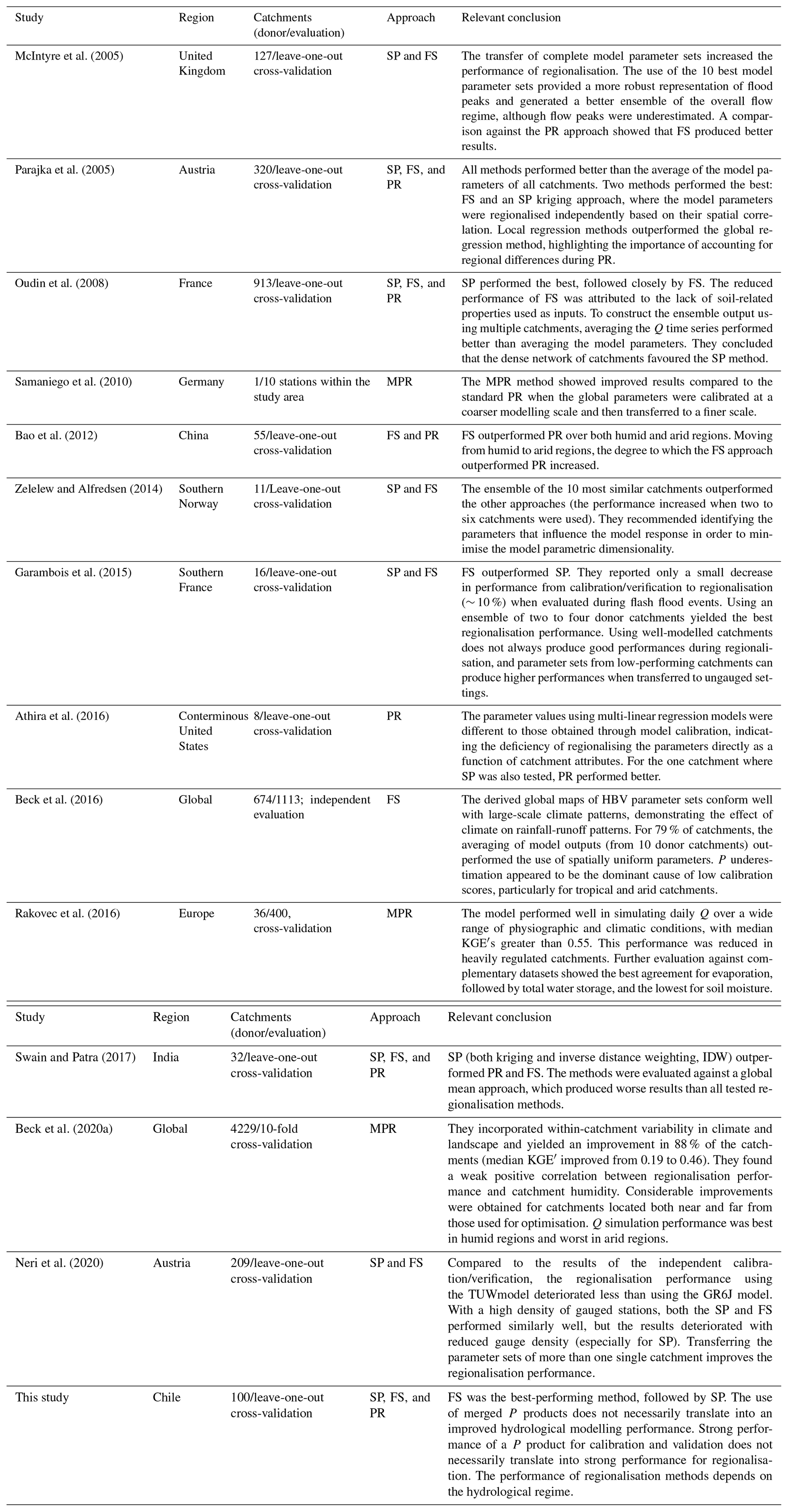
Most regionalisation studies have been conducted over regions with a dense network of meteorological stations (see Table 1), including Europe (e.g. McIntyre et al., 2005; Parajka et al., 2005; Oudin et al., 2008; Singh et al., 2012; Zelelew and Alfredsen, 2014; Garambois et al., 2015; Rakovec et al., 2016; Neri et al., 2020), the conterminous United States (Athira et al., 2016; Saadi et al., 2019), India (Swain and Patra, 2017), and China (Bao et al., 2012). However, in developing countries, P has traditionally been estimated through interpolation within sparse rain gauge networks, which is subject to large uncertainties (Hofstra et al., 2010; Woldemeskel et al., 2013; Adhikary et al., 2015; Xavier et al., 2016), hindering an accurate spatio-temporal representation of P patterns. Over the last decades, the emergence of near-global and high-resolution gridded P products has introduced new possibilities for hydrological modelling in data-scarce regions (Maggioni and Massari, 2018; Sun et al., 2018), despite these products still being affected by systematic, random, and detection errors (Ren and Li, 2007; Sevruk et al., 2009; Zambrano-Bigiarini et al., 2017; Baez-Villanueva et al., 2018), which are more pronounced over mountainous regions (Maggioni and Massari, 2018; Beck et al., 2019). Although hydrological model calibration can partly compensate for errors in the representation of P (Elsner et al., 2014; Maggioni and Massari, 2018), this may lead to unrealistic model behaviour (Nikolopoulos et al., 2013; Xue et al., 2013; Ciabatta et al., 2016), thus affecting the quality of parameter regionalisation results.

To date, few regionalisation studies have used gridded P products at the daily temporal scale. Beck et al. (2016) used the Climate Prediction Center unified gauge-based P product (CPC) to provide spatially distributed HBV parameters at the global scale. They selected CPC because it yielded better performance than ERA-Interim during calibration. Rakovec et al. (2016) used the European daily high-resolution gridded dataset (E-OBSv8.0) to force a mesoscale hydrological model over 400 catchments in Europe, providing regionalised model parameters through a multivariate parameter estimation technique. More recently, Beck et al. (2020a) combined MSWEPv2.2 with a novel multiscale parameter regionalisation approach to provide global gridded parameter estimates using daily Q observations from 4229 catchments. Although these studies have successfully used gridded P products for parameter regionalisation, they only selected one product, and thus the effects that the choice of a P dataset can have on regionalisation results remain unknown. This study aims to answer the following questions:

• (i)

  To what extent does the choice of gridded P forcing used in calibration affect the relative performance of regionalisation techniques?

• (ii)

  How does this relative performance vary across catchments with different hydrological regimes?

McIntyre et al. (2005)Parajka et al. (2005)Oudin et al. (2008)Samaniego et al. (2010)Bao et al. (2012)Zelelew and Alfredsen (2014)Garambois et al. (2015)Athira et al. (2016)Beck et al. (2016)Rakovec et al. (2016)Swain and Patra (2017)Beck et al. (2020a)Neri et al. (2020)

Table 1 Summary of selected regionalisation studies that used spatial proximity (SP), feature similarity (FS), parameter regression (PR), or multiscale parameter regionalisation (MPR). This study has been added for completeness.

2 Study area and selection of catchments

Our study domain is continental Chile (Fig. 1), which is bounded to the west by the Pacific Ocean, to the north by Peru, and to the east by Bolivia and Argentina. The territory spans 4300 km of latitudinal extension (17.5–56.0^∘ S) and on average 180 km of longitudinal extension (76.0–66.0^∘ W), with elevation (Jarvis et al., 2008) ranging from 0 to 6892 m a.s.l. in the Andes Mountains. Figure 1 shows the elevation, land cover (Zhao et al., 2016), Köppen–Geiger climate classification (Beck et al., 2018), and hydrological regimes for the five major macroclimatic zones presented in Zambrano-Bigiarini et al. (2017). A large variety of climates are present across the country, with the macroclimatic zones transitioning from the (hyper)arid and semi-arid climates in the Far North (17.50–26.00^∘ S) and Near North (26.00–32.18^∘ S), through temperate climates in Central Chile (32.18–36.40^∘ S), to more humid and polar climates in the South (36.40–43.70^∘ S) and Far South (43.70–56.00^∘ S). P increases with elevation and latitude (in the southern direction), ranging from almost zero in the Atacama Desert to ∼6000 mm yr⁻¹ in the surroundings of Puerto Cárdenas (∼43.2^∘ S). Similar to the P patterns, both the mean annual Q and rainfall-runoff ratio tend to increase from north to south (Alvarez-Garreton et al., 2018; Vásquez et al., 2021).

The El Niño–Southern Oscillation (ENSO) has a large impact on winter P, with negative anomalies during La Niña and positive anomalies during El Niño events (Verbist et al., 2010; Robertson et al., 2014). Although neutral ENSO conditions have prevailed since 2011 (except for a strong El Niño event during 2015), an uninterrupted sequence of dry years with increased temperatures has been observed from 2010–2018, with annual P deficits of about 25 %–45 % across Chile. This long-term deficit in P volume, also known as the Chilean megadrought (Boisier et al., 2016; Garreaud et al., 2017), has reduced snow cover, river flows, reservoir storage, and groundwater levels across Chile (Garreaud et al., 2017, 2020).

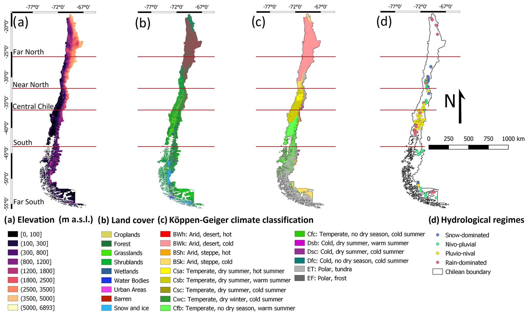
Figure 1 Study area: (a) elevation (SRTMv4.1; Jarvis et al., 2008); (b) land cover classification (Zhao et al., 2016); (c) Köppen–Geiger climate classification (Beck et al., 2018); and (d) hydrological regimes of the selected catchments over the five major macroclimatic zones according to Zambrano-Bigiarini et al. (2017).

Hydroclimatic indices and characteristics for 516 catchments in continental Chile were acquired from the Catchment Attributes and MEteorology for Large-sample Studies dataset in Chile (CAMELS-CL; Alvarez-Garreton et al., 2018). The dataset includes location, topography, geology, soil types, land cover, hydrological signatures, and human intervention degree, among others. Q data were obtained from the Center for Climate and Resilience Research (CR2; http://www.cr2.cl/datos-de-caudales/, last access: October 2020) for 1930–2018 because Q data from CAMELS-CL ended in 2016 at the time of conducting this study. We selected the near-natural catchments from the CAMELS-CL database that fulfilled the following criteria:

1. less than 25 % of missing values in the daily Q time series for 1990–2018 (may be non-consecutive)

2. absence of large dams (big_dam = 0)

3. less than 10 % of Q allocated to consumptive uses (interv_degree < 0.1)

4. not dominated by glaciers (lc_glacier < 5 %)

5. less than 5 % of the area defined as urban (imp_frac < 5 %)

6. absence of substantial irrigation abstractions (crop_frac < 20 %)

7. less than 20 % of the area covered by forest plantations (fp_frac < 20 %)

8. no signs of artificial regulation in the hydrograph (10 excluded in total).

The drainage areas of the selected catchments (100) range from 35 to 11 137 km², with a median value of 645 km². The selected catchments contain 42 nested catchments (i.e. catchments that are contained in a larger catchment). We adjusted the classification of these catchments according to hydrological regime, building on the classifications presented in several national and regional technical reports (e.g. DGA, 1998, 1999, 2004a, b, c, 2006, 2016a, b, 2018), by visually analysing the contribution of solid and liquid P to the mean monthly Q values. These regimes were classified as (i) snow-dominated; (ii) nivo-pluvial, i.e. snow-dominated with a rain component; (iii) pluvio-nival, i.e. rain-dominated with a snow component; and (iv) rain-dominated, as shown in Fig. 1d. Figure A1 shows conceptual hydrographs for each of these regimes and is presented in Appendix A.

3 Methods

3.1 Meteorological forcings

3.1.1 Precipitation products

Four P products were used to investigate how the choice of P forcing affects the performance of regionalisation techniques. The P products are presented in Table 2 and were selected because previous studies have reported good agreement when evaluated against in situ measurements over continental Chile (Zambrano-Bigiarini et al., 2017; Boisier et al., 2018; Baez-Villanueva et al., 2018, 2020).

Boisier et al. (2018)Baez-Villanueva et al. (2020)Hersbach et al. (2020)Beck et al. (2017b, 2019)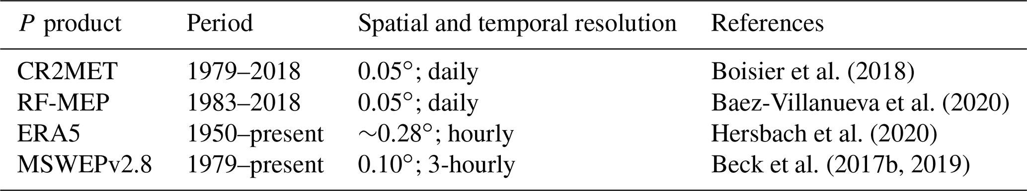

Table 2 Gridded P products used in this study.

The Center for Climate and Resilience Research Meteorological dataset version 2.0 (CR2MET; Boisier et al., 2018) provides daily gridded P estimates over continental Chile at a 5 km spatial resolution for 1979–2018. These estimates are produced by combining rain gauge observations with reanalysis data from ERA5, while CR2MET version 1.0 of this product was produced using ERA-Interim data (Boisier et al., 2018). As CR2MET was developed specifically for Chile and uses all the Chilean rain gauges (874 across Chile; see Fig. S1 in the Supplement), it is considered as the “reference” P product of Chile.

The random forest merging procedure (RF-MEP; Baez-Villanueva et al., 2020) combines gridded P products, ground-based measurements, and other spatial covariates to generate P estimates. We applied this methodology to generate a spatially distributed, daily P product for continental Chile, using daily records from 334 rain gauges (obtained from CR2; http://www.cr2.cl/datos-de-precipitacion/, last access: 10 January 2021), gridded P data from the ERA5 reanalysis (Hersbach et al., 2020) aggregated to the Chilean time, and elevation (SRTMv4.1; Jarvis et al., 2008) as covariates. This RF-MEP version 2 product (hereafter, RF-MEP) was generated for 1990–2018 with a spatial resolution of 0.05^∘ using the RFmerge R package (Zambrano-Bigiarini et al., 2020).

ERA5 (Hersbach et al., 2020) is a reanalysis product that provides hourly P estimates (as well as other variables) from 1950 to present at a spatial resolution of around 30 km (∼ 0.28^∘). There are important improvements in its P estimates compared to its predecessor ERA-Interim, such as improved (i) representation of mixed-phase clouds, (ii) prognostics variables for rain and snow, (iii) parameterisation of microphysics, and (iv) representation of tropical variability (Hersbach et al., 2020). Although ERA5 also assimilates NCEP Stage IV P estimates over the conterminous United States, which combine NEXRAD data with in situ measurements, it does not incorporate information from any ground-based P stations over Chile. Hourly ERA5 estimates were aggregated into daily P values, taking into account the reporting times of the Chilean rain gauges (08:00–07:59 local time, which represents 11:00–10:59 UTC). Although this product has a relatively low spatial resolution compared to the other selected products, we included it because (i) Chile is dominated by large-scale, frontal systems (Zhang and Wang, 2021), and therefore, coarse-resolution products may perform well even over small catchments; (ii) reanalysis products tend to perform well at high latitudes (Beck et al., 2017a); and (iii) we consider that its inclusion represents a realistic situation that may exist in many practical applications (i.e. where a catchment size is small relative to P product resolution).

The Multi-Source Weighted-Ensemble Precipitation (MSWEPv2.8; Beck et al., 2017b, 2019) is a 3-hourly P product with a spatial resolution of 0.10^∘, which takes advantage of the complementary strengths of satellite, reanalysis, and ground-based data. MSWEPv2.8 applies daily and monthly corrections to its estimates using data from around 77 000 rain gauge stations globally (628 of these are over Chile; see Fig. S1), accounting for their local reporting times. The 3-hourly MSWEPv2.8 estimates were also aggregated into daily P to account for the difference in the reporting times.

Figure 2a shows the spatial distribution of mean annual P for all products over 1990–2018, while Fig. 2b shows box plots of the mean monthly P averaged over catchments located within each macroclimatic zone. All P products show relatively similar patterns of spatial variability across continental Chile; however, there are substantial differences in their total P amounts. In general, P increases from the (hyper-arid) Far North to the South and decreases again in the Far South. P also increases from the west coast towards the Andes Mountains. ERA5 provides higher P amounts over all five macroclimatic zones, while RF-MEP generally yields the lowest annual P values. Over the Far North, all products show a marked rainy season during December–March due to summer convective P, which differs from the marked seasonality evident over the Near North, Central Chile, and South regions. Over the Far North, ERA5 presents the highest mean annual P (157 mm), which is almost twice the amount provided by the second-highest product MSWEPv2.8 (83 mm), followed by CR2MET (63 mm), while RF-MEP has the lowest mean annual P (40 mm). Although ERA5 presents the highest mean annual P values over the Near North, Central Chile, and South regions (208, 902, and 2172 mm, respectively), when considering only our case study catchments (Fig. 2b), CR2MET has the highest mean monthly values over the Central Chile and South regions during April–June. RF-MEP and MSWEPv2.8 have similar mean annual P values over Central Chile (670 mm for both products) and the South (1670 and 1735 mm, respectively) regions, although RF-MEP consistently shows the largest monthly P amounts of the two products over the corresponding catchments. ERA5 provides the highest mean annual P values over the Far South (3018 mm), followed by CR2MET (1888 mm), MSWEPv2.8 (1714 mm), and RF-MEP (815 mm). Finally, each product shows low seasonality over the Far South. Here, ERA5 presents higher monthly P values throughout the year, with the largest difference from the other products between January–March and September–December.

To gain a deeper understanding of the differences between the four P products, we examined the spatial distribution of median annual values of four Climdex indices (Karl et al., 1999) for 1990–2018 (Fig. 3). First, to account for days without rain (P<1 mm), we used the consecutive dry days index (CDD; Fig. 3a), which retrieves the maximum dry spell length. It is evident that CR2MET yields longer dry spells, mainly across the Far North and Near North regions, while ERA5 has shorter dry spells over these regions, especially over the Andes Mountains. CR2MET, RF-MEP, and MSWEPv2.8 have similar spatial patterns over the Central Chile and South regions, while ERA5 has fewer consecutive dry days over the Andes Mountains. Similarly, ERA5 provides shorter dry spells over the Far South, while CR2MET and RF-MEP present similar patterns. These results are consistent with the consecutive wet days index (CWD; Fig. 3b), which assesses the frequency and intermittency of P. ERA5 provides the highest CWD values over the driest regions (Far North and Near North), with medians ranging from 0 to 25 d, followed by MSWEPv2.8 (0 to 15 d). ERA5 also shows higher CWD values over high-elevation areas in Central Chile, while the remaining products show similar spatial patterns to each other. The four products show agreement in the CWD over the South region, with values ranging from 5 to 25 d. Finally, RF-MEP shows the lowest consecutive days with P in the Far South, followed by CR2MET and MSWEPv2.8, while ERA5 shows substantially higher CWD values at latitudes greater than 47^∘ S.

To characterise high P intensities, we used the Rx5day (Fig. 3c) and R95pTOT (Fig. 3d) indices, which represent the maximum P accumulated over 5 consecutive days and the total P above the 95th percentile of the daily P for wet days, respectively. Figure 3c shows that ERA5 and CR2MET generally yield the highest Rx5day values, followed by MSWEPv2.8 and RF-MEP. A similar spatial variability is obtained with R95pTOT (Fig. 3d), indicating that there is a greater contribution of P from extreme events in ERA5 over high-elevation areas. These spatial patterns are replicated to some extent by CR2MET, which provides R95pTOT values up to 1200 mm over the Andes Mountains in Central Chile.

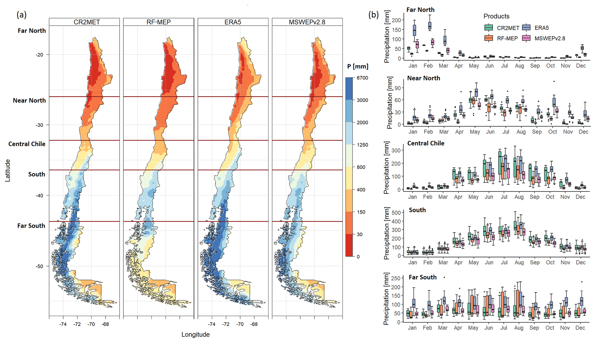
Figure 2 Comparison of P products over 1990–2018 (full time period): (a) mean annual P for each product resampled to a 0.05^∘ spatial resolution using the nearest neighbour method. The dark red horizontal lines represent the limits of each major macroclimatic zone and (b) mean monthly P averaged over each catchment located within each macroclimatic zone (see Fig. 1d).

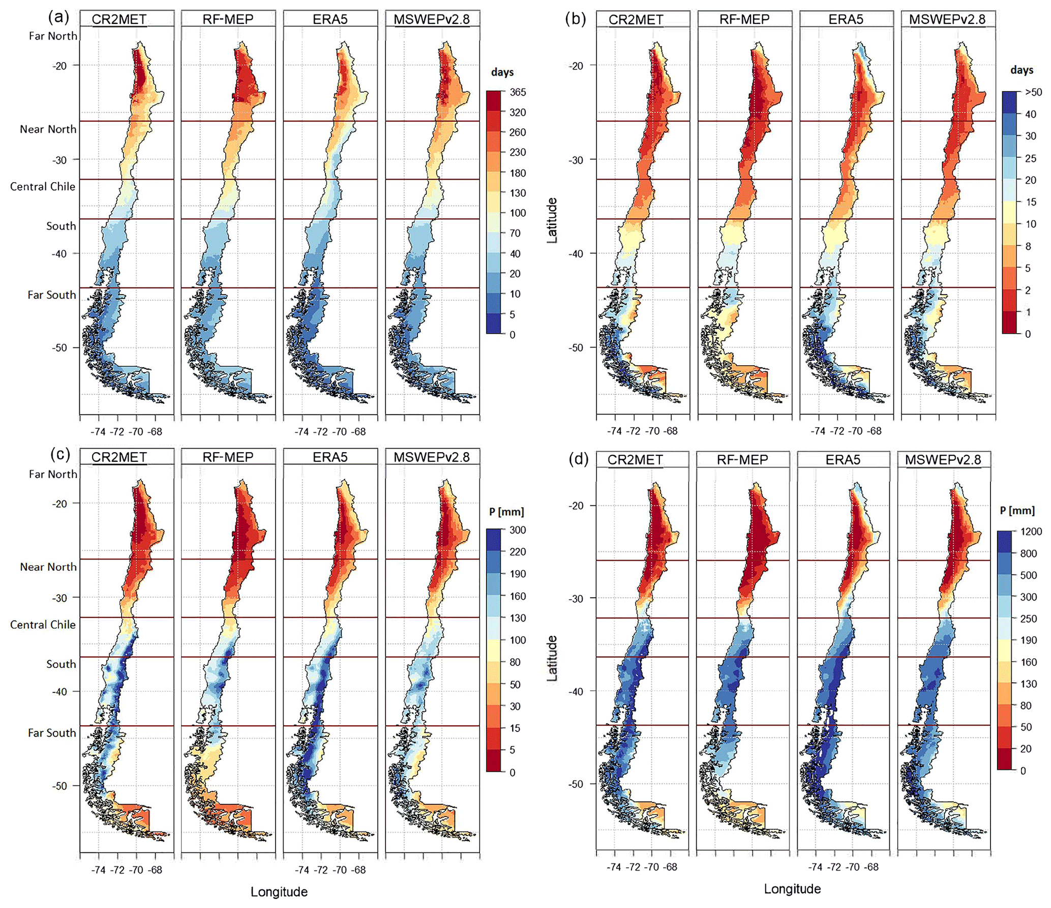
Figure 3 Median annual values of four Climdex indices over 1990–2018 (full period): (a) number of consecutive dry days (CDD), (b) number of consecutive wet days (CWD), (c) maximum P over five consecutive days (Rx5day), and (d) annual P that is above the 95th percentile of P for wet days (R95pTOT). The dark red horizontal lines represent the limits of each macroclimatic zone.

3.1.2 Air temperature and potential evaporation

Maximum and minimum daily air temperature (T) at a spatial resolution of 0.05^∘ were taken from CR2MET. T is estimated using multivariate regression from the Moderate Resolution Imaging Spectroradiometer (MODIS) land surface temperature (LST) and ERA5 estimates as covariates (Alvarez-Garreton et al., 2018; Boisier et al., 2018). The Hargreaves–Samani equation (Hargreaves and Samani, 1985) was used to obtain daily potential evaporation (PE) from CR2MET maximum and minimum daily T at the same spatial resolution (0.05^∘).

3.2 Hydrological model

The TUWmodel (Viglione and Parajka, 2020) is a conceptual hydrological model that follows the structure of the Hydrologiska Byråns Vattenbalansavdelning (HBV) model (Bergström, 1976, 1995; Lindström, 1997). The model simulates the catchment-scale water balance at daily time steps, including processes related to snow accumulation and melting, change of moisture in the soil profile, and surface flow in the drainage network. The TUWmodel was validated over 320 catchments in Austria (Parajka et al., 2007) and has subsequently been used in numerous studies (e.g. Parajka et al., 2016; Zessner et al., 2017; Melsen et al., 2018; Sleziak et al., 2020). We selected a HBV-like conceptual model because it has shown good results in (i) many regionalisation studies (e.g. Parajka et al., 2005; Singh et al., 2012; Beck et al., 2016; Neri et al., 2020) and (ii) catchments with diverse hydroclimatic and geomorphological characteristics (Vetter et al., 2015; Ding et al., 2016; Unduche et al., 2018; Huang et al., 2019).

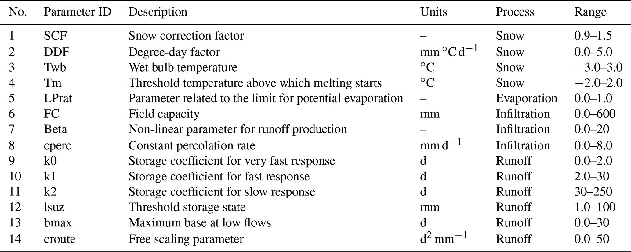
The TUWmodel requires as inputs daily time series of P, T, and PE. The parameters used by the TUWmodel to represent the hydrological processes are listed in Table 3, including the ranges selected for model calibration, which were adopted from previous studies (Parajka et al., 2007; Ceola et al., 2015) that calibrated the TUWmodel over a large number of mountainous catchments with snow influence. We ran the TUWmodel with a semi-distributed configuration for the period 1990–2018 based on meteorological and Q data availability. For each catchment, the number of equal-area elevation bands (EZ) was defined as $\text{EZ}=(H_{\max }-H_{\min })/\mathrm{200}$, where H represents elevation. In cases where EZ>10, EZ was set to 10 to reduce the computational demand of the simulations. Furthermore, in catchments with H_min below 900 m a.s.l., the upper bound of the first EZ band was set to 900 m under the assumption that there is no snow influence below this elevation for the particular case of continental Chile. For more details about the TUWmodel implementation in R and the comparison of different HBV-like models, readers are referred to Astagneau et al. (2021) and Jansen et al. (2021), respectively.

Table 3 Summary of the TUWmodel parameters considered for calibration, following the conceptualisation presented in Széles et al. (2020).

3.3 Independent catchment calibration and verification

The simulation period used for this study was 1990–2018. For calibration purposes, we used the first 10 years as a conservative warm-up period to initialise the model stores, as in Beck et al. (2020a). The calibration period (2000–2014) includes near-normal conditions and the beginning of the Chilean megadrought. The first evaluation period (hereafter Verification 1, 1990–1999) represents near-normal/wet hydroclimatic conditions, while the second evaluation period (hereafter Verification 2, 2015–2018) spans the second half of the Chilean megadrought and was used to test the ability of the hydrological simulations to represent dry conditions. To initialise model stores for the Verification 1 period, we used an 8-year warm-up period due to P product availability. We replicated Figs. 2 and 3 for these three periods to analyse the differences between the selected P products (see the Supplement, Figs. S2–S7).

We used the modified Kling–Gupta efficiency (KGE^′, Eq. 1; Kling et al., 2012) to calibrate the TUWmodel, which typically provides better hydrograph simulations than other squared-error indices (Gupta et al., 2009; Kling et al., 2012; Mizukami et al., 2019) and has been used in numerous studies (e.g. Garcia et al., 2017; Beck et al., 2019; Baez-Villanueva et al., 2020; Neri et al., 2020; Széles et al., 2020). The KGE^′ has three components: the Pearson correlation coefficient (r; Eq. 2), the bias ratio (β; Eq. 3), and the variability ratio (γ; Eq. 4). μ is the mean Q, CV is the coefficient of variation, σ represents the standard deviation of Q, and the subscripts “s” and “o” represent simulated and observed Q, respectively. The KGE^′ and its components have their optimum value at 1, and its optimisation seeks to reproduce the temporal dynamics (measured by r) while preserving the volume and variability of Q, measured by β and γ, respectively (Kling et al., 2012).

$$\begin{array}{}\text{(1)}& {\displaystyle }{\text{KGE}}^{\prime }=\mathrm{1}-\sqrt{(r-\mathrm{1}{)}^{\mathrm{2}}+(\mathit{\beta }-\mathrm{1}{)}^{\mathrm{2}}+(\mathit{\gamma }-\mathrm{1}{)}^{\mathrm{2}}}\text{(2)}& {\displaystyle }r={\displaystyle \frac{{\sum }_{i=\mathrm{1}}^n(O_i-\overline{O})(S_i-\overline{S})}{\sqrt{{\sum }_{i=\mathrm{1}}^n(O_i-\overline{O}{)}^{\mathrm{2}}}\sqrt{{\sum }_{i=\mathrm{1}}^n(S_i-\overline{S}{)}^{\mathrm{2}}}}}\text{(3)}& {\displaystyle }\mathit{\beta }={\displaystyle \frac{{\mathit{\mu }}_{\mathrm{s}}}{{\mathit{\mu }}_{\mathrm{o}}}}\text{(4)}& {\displaystyle }\mathit{\gamma }={\displaystyle \frac{{\text{CV}}_{\mathrm{s}}}{{\text{CV}}_{\mathrm{o}}}}={\displaystyle \frac{{\mathit{\sigma }}_{\mathrm{s}}/{\mathit{\mu }}_{\mathrm{s}}}{{\mathit{\sigma }}_{\mathrm{o}}/{\mathit{\mu }}_{\mathrm{o}}}}\end{array}$$

To calibrate the model parameters, we used the hydroPSO global optimisation algorithm (Zambrano-Bigiarini and Rojas, 2013), which implements a state-of-the-art version of the particle swarm optimisation technique (PSO; Eberhart and Kennedy, 1995; Kennedy and Eberhart, 1995). We used the standard PSO 2011 algorithm (Clerc, 2011a, b), defined as spso2011 in the hydroPSO R package (Zambrano-Bigiarini and Rojas, 2013). We set the number of particles in the swarm (npart = 80), the maximum number of iterations (maxit = 100), and the relative convergence tolerance (reltol = $\mathrm{1}\times {\mathrm{10}}^{-\mathrm{10}}$), while the default values were used for all other parameters. Over the last decade, hydroPSO has been successfully used to calibrate numerous hydrological and environmental models (e.g. Brauer et al., 2014; Silal et al., 2015; Bisselink et al., 2016; Kundu et al., 2017; Kearney and Maino, 2018; Abdelaziz et al., 2019; Ollivier et al., 2020; Hann et al., 2021). For more details on the use of the hydroPSO package to calibrate the TUWmodel, readers are referred to Zambrano-Bigiarini and Baez-Villanueva (2020).

3.4 Regionalisation techniques

After obtaining catchment-specific model parameters through independent catchment calibration (Sect. 3.3), we compared three parameter regionalisation techniques: (i) spatial proximity, (ii) feature similarity, and (iii) parameter regression. We assessed performance through a leave-one-out cross-validation exercise, which consists of leaving out each one of the 100 catchments, transferring model parameters, conducting Q simulations, and computing performance evaluation metrics.

3.4.1 Spatial proximity

The spatial proximity method assumes that climatic and physical characteristics are relatively homogeneous over a region (Oudin et al., 2008). We quantified the spatial proximity between the target pseudo-ungauged and the remaining catchments using the Euclidean distance between catchment centroids, computed with geographic coordinates (i.e. latitude and longitude):

$$\begin{array}{}\text{(5)}& {\text{ED}}_{ij}=\sqrt{\sum _{k=\mathrm{1}}^n(x_{k,i}-x_{k,j}{)}^{\mathrm{2}}}.\end{array}$$

For each pseudo-ungauged catchment, the donor was chosen according to the minimum Euclidean distance, and the full parameter set obtained during the independent calibration of the donor catchment was transferred to the pseudo-ungauged catchment.

3.4.2 Feature similarity

In the feature similarity method, we transferred the calibrated parameter sets from 10 donor catchments to the pseudo-ungauged catchment based on similarity between climatic and geomorphological features, quantified using the catchment characteristics presented in Table 4. To exclude redundant information, we first performed correlation analyses between catchment descriptors using the Pearson and Spearman rank correlation coefficients (to account for linear and monotonic correlation, respectively) and discarded three descriptors with high correlations (mean elevation, mean annual PE, and the Simple Precipitation Intensity Index (SDII); see Appendix B). Also, we discarded snow cover because it was found to be unreliable, leaving nine catchment features for this method. To assign equal weight to each catchment characteristic, they were normalised into the range [0, 1] using Eq. (6):

$$\begin{array}{}\text{(6)}& Z_f={\displaystyle \frac{x_f-x_{\min }}{x_{\max }-x_{\min }}},\end{array}$$

where x_f is the value of the characteristic for catchment f, while x_max and x_min are the maximum and minimum values of the characteristic x over all catchments. After normalising all catchment characteristics, we calculated the dissimilarity as follows:

$$\begin{array}{}\text{(7)}& S_{i,j}=\sum _{m=\mathrm{1}}^n\mid Z_{i,m}-Z_{j,m}\mid ,\end{array}$$

where S_i,j is the dissimilarity index between catchments i and j; Z_i,m and Z_j,m are the normalised values of the m catchment characteristic for catchments i and j, respectively; and n is the total number of characteristics.

Table 4 Selected climatic and physiographic characteristics to quantify feature similarity between catchments. All variables related to P were computed using the corresponding P product used as an input to the TUWmodel for 1990–2018.

For each pseudo-ungauged catchment i, the 10 catchments j with the lowest dissimilarity indices (S_i,j) were selected as donors (Oudin et al., 2008; Zhang and Chiew, 2009; Zhang et al., 2015; Beck et al., 2016). The full parameter sets obtained during the independent calibrations of each donor catchment were used to run TUWmodel in the pseudo-ungauged catchment, thus producing an ensemble of 10 Q simulations, as in previous studies (McIntyre et al., 2005; Zelelew and Alfredsen, 2014; Beck et al., 2016). The 10 Q time series were then averaged to produce a single Q time series.

3.4.3 Parameter regression

The parameter regression technique aims to detect statistical relationships between parameter values and catchment characteristics and uses these relationships to estimate model parameters for ungauged catchments (Parajka et al., 2005; Oudin et al., 2008; Swain and Patra, 2017). To account for non-linear relationships between model parameters and catchment characteristics, we implemented the random forest machine learning algorithm (RF; Breiman, 2001; Prasad et al., 2006; Biau and Scornet, 2016) provided in the RandomForest R package (Liaw and Wiener, 2002). RF uses an ensemble of decision trees between predictand and predictor values (also known as covariates) for regression and supervised classification and has the capability to deal with high-dimensional feature spaces and small sample sizes (Biau and Scornet, 2016). Previous studies have shown that RF can deal with several covariates as well as non-informative predictors because it does not lead to overfitting or biased estimates (Díaz-Uriarte and Alvarez de Andrés, 2006; Biau and Scornet, 2016; Hengl et al., 2018), which is why it has been used for numerous hydrological applications (Saadi et al., 2019; Baez-Villanueva et al., 2020; Beck et al., 2020b; Zhang et al., 2021). For a more detailed description of RF, we refer the reader to Prasad et al. (2006), Biau and Scornet (2016), and Addor et al. (2018).

For this study, we developed one RF model for each TUWmodel parameter, using all 13 independent catchment characteristics listed in Table 4 as covariates. Our experimental setup used an ensemble of 2000 regression trees, a minimum of five terminal nodes for each model, and $p/\mathrm{3}$ variables randomly sampled as candidates at each split, where p represents the number of predictors. The trained RF models were then used to predict parameter values in the pseudo-ungauged catchments.

3.5 Influence of nested catchments

To evaluate the influence of nested catchments on the performance of the three regionalisation methods, we repeated the three regionalisation methods for each target catchment, with catchments considered to be nested (in relation to the pseudo-ungauged catchment) excluded from the set of potential donor catchments. Following Neri et al. (2020), we used a cut-off point of 10 % of drainage area, meaning that only catchments that cover more than 10 % of the area of the parent catchment were considered to be nested.

3.6 Influence of donor catchments for feature similarity

To evaluate the influence of the number of donors used in feature similarity, we repeated the process followed in Sect. 3.4.2 to assess the performance of this regionalisation method when 1, 2, 4, 6, 8, and 10 donor catchments are selected. This analysis evaluates the impact of averaging varying numbers of simulations compared to the results that are based on only the most similar catchment.

We performed all analyses using the R Project of Statistical Computing (R Core Team, 2020). In addition to the R packages described in the methodology, we used the hydroGOF (Zambrano-Bigiarini, 2020a), hydroTSM (Zambrano-Bigiarini, 2020b), lfstat (Koffler et al., 2016), raster (Hijmans, 2020), rasterVis (Perpiñán and Hijmans, 2020), rgdal (Bivand et al., 2020), and rgeos (Bivand and Rundel, 2020) packages.

4 Results

4.1 Performance of P products

4.1.1 Calibration and verification

Figure 4 shows the performance of the TUWmodel during calibration (2000–2014) and the two verification periods (1990–1999 and 2015–2018), prior to any regionalisation procedure. CR2MET provided the best performance for all evaluated periods, with median KGE^′s of 0.84, 0.76, and 0.66, for calibration, Verification 1 (1990–1999, near-normal/wet), and Verification 2 (2015–2018, dry), respectively, followed closely by RF-MEP. Surprisingly, MSWEPv2.8 provided the poorest performance for calibration and Verification 1. For all P products, the lowest performances were obtained during the (dry) Verification 2 period, emphasising the challenges of estimating Q in dry conditions, as discussed by Maggioni et al. (2013) and Beck et al. (2016). Despite the substantial variations between P products (see Sect. 3.1.1), the TUWmodel performed well for all P products in the calibration, Verification 1, and Verification 2 periods, with median KGE^′ values greater than 0.77, 0.71, and 0.62, respectively. The calibrated model parameters lay well within the selected parameter ranges in the large majority of the cases (see Fig. S8 of the Supplement). In other words, the selected parameter ranges were wide enough so that calibrated parameter values were not concentrated at their lower or upper limits.

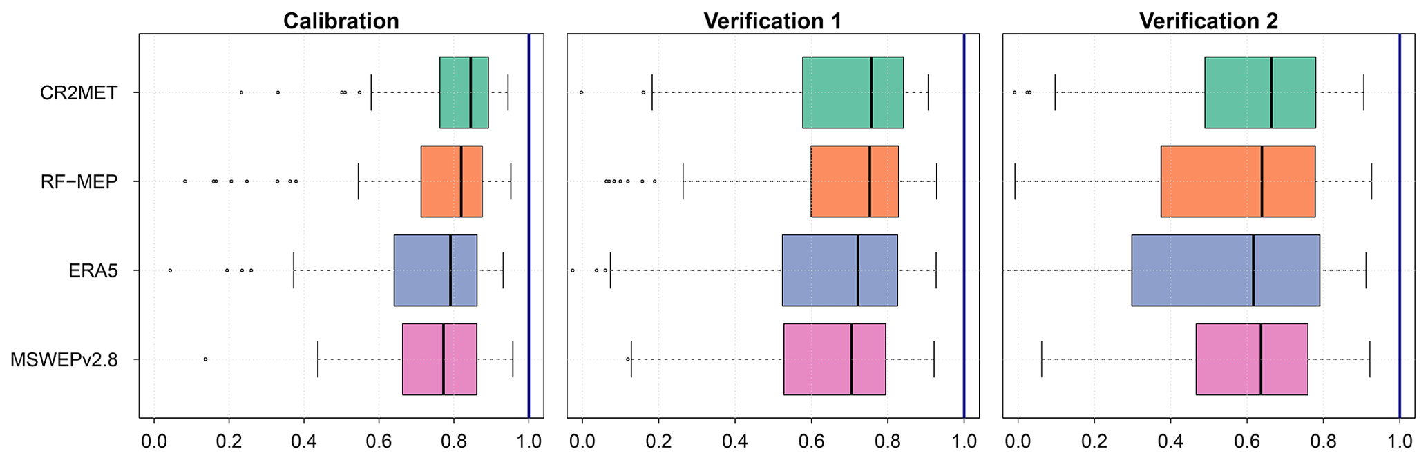
Figure 4 Performance of the TUWmodel during the calibration (2000–2014), Verification 1 (1990–1999), and Verification 2 (2015–2018), prior to any regionalisation, using the modified Kling–Gupta efficiency (KGE^′). The solid line represents the median value, the edges of the boxes represent the first and third quartiles, and the whiskers extend to the most extreme data point which is no more than 1.5 times the interquartile range from the box. The blue line indicates the optimal value for the KGE^′.

Figure 5 shows the performance of the TUWmodel during calibration, Verification 1, and Verification 2 per hydrological regime (see Fig. 1d). The TUWmodel performed better over the pluvio-nival catchments, with median KGE^′ values above 0.77, 0.76, and 0.69 for calibration, Verification 1, and Verification 2, respectively. During the calibration period, there was no clear second best regime. For instance, the snow-dominated catchments presented slightly higher median KGE^′ values but a more pronounced dispersion, while the pluvio-nival and rain-dominated catchments presented lower dispersion but reduced median values. The snow-dominated catchments presented a more pronounced decrease from calibration (median KGE${}^{\prime }>\mathrm{0.85}$) to both verification periods (>0.55 and 0.23 for Verification 1 and Verification 2, respectively). During both verification periods, the rain-dominated catchments presented the highest dispersion increases in both verification periods compared to calibration.

Over the snow-dominated catchments, ERA5 performed the worst as it presented the highest dispersion and the lowest median KGE^′ values during Verification 1 (0.55) and Verification 2 (0.25), despite having the highest median KGE^′ during calibration (0.87). RF-MEP performed the best during Verification 1 (0.68), while MSWEPv2.8 performed the best during the dry Verification 2 period (median KGE^′ of 0.60). CR2MET performed the best over the nivo-pluvial catchments, with median KGE^′ values above 0.64, while RF-MEP performed relatively worse for both verification periods, with median KGE^′ values above 0.48 and a larger dispersion than the other products, despite having a similar median KGE^′ (0.62) in Verification 1 to ERA5 and MSWEPv2.8 (0.61, and 0.60, respectively). Over the pluvio-nival catchments, all products showed a relatively good performance, with CR2MET being the best P product in calibration and Verification 1 (median KGE^′s of 0.87 and 0.84, respectively), while ERA5 performed the best during Verification 2 (median KGE^′ of 0.78). RF-MEP performed the best over the rain-dominated catchments in calibration and Verification 1, with median KGE^′ values of 0.84 and 0.77, respectively, while ERA5 performed the worst (median KGE^′ values of 0.69 and 0.70). Finally, CR2MET performed the best in Verification 2 (median KGE^′ of 0.72), followed by MSWEPv2.8 (median KGE^′ of 0.69).

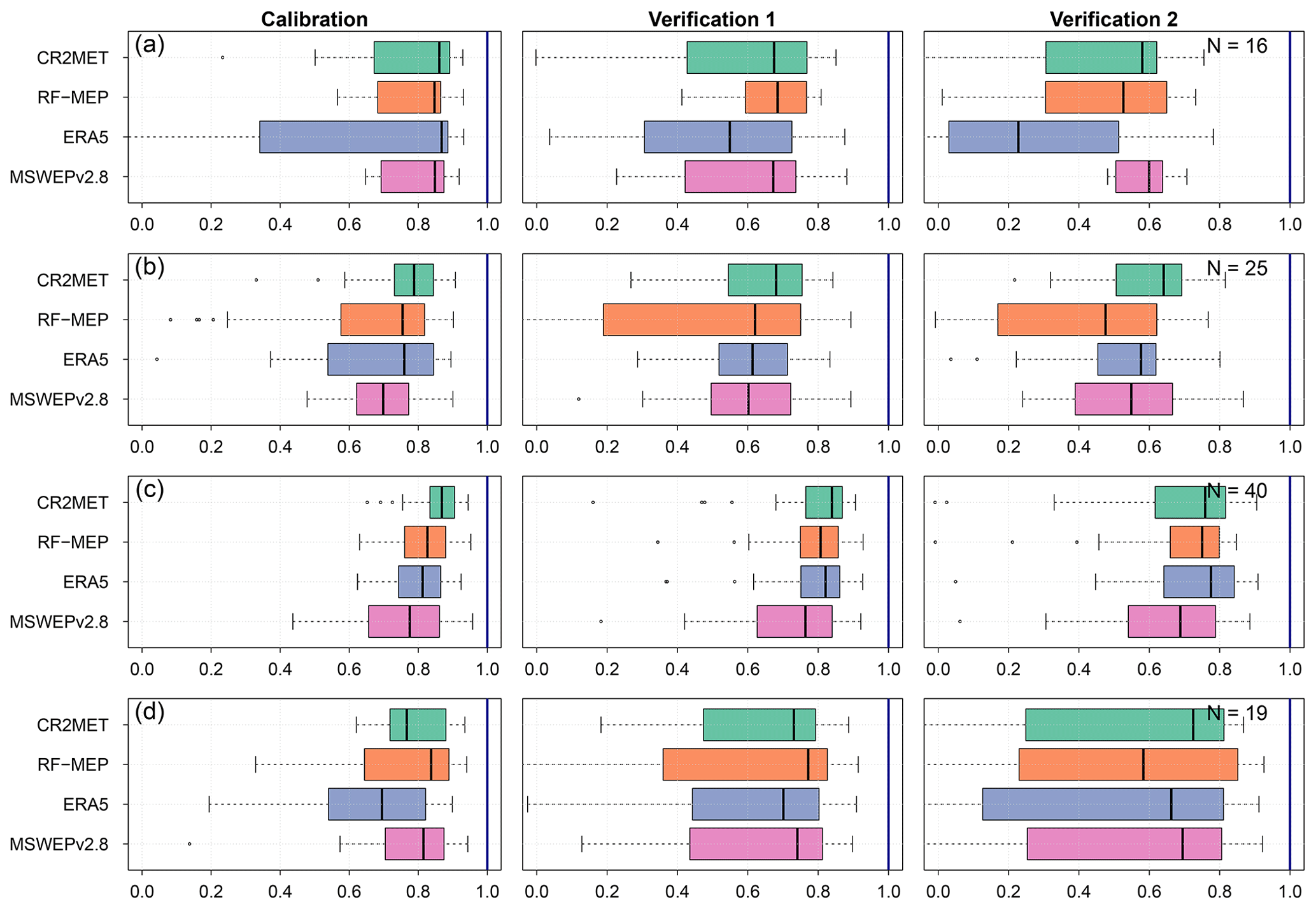
Figure 5 Performance of TUWmodel during calibration (2000–2014), Verification 1 (1990–1999), and Verification 2 (2015–2018), prior to any regionalisation, over catchments with different hydrological regimes: (a) snow-dominated, (b) nivo-pluvial, (c) pluvio-nival, and (d) rain-dominated.

4.1.2 Performance during regionalisation

Figure 6 summarises the leave-one-out cross-validation results obtained from the application of three regionalisation methods, for each P product. The results are displayed for the calibration (2000–2014; panel a), Verification 1 (1990–1999; panel b), and Verification 2 (2015–2018; panel c) periods. Overall, the median performance of all P products was the best for feature similarity, with median KGE^′ values between 0.44–0.62 for all periods, followed by spatial proximity (0.39–0.55) and parameter regression (−0.12–0.51). In addition to exhibiting a considerably lower overall performance, parameter regression returned a larger spread in KGE^′s for all periods.

The overall performances obtained for feature similarity and spatial proximity are relatively close for different P products over each period (Fig. 6). For feature similarity, all P products generate acceptable KGE^′ results (median KGE${}^{\prime }>\mathrm{0.54}$) during the calibration and Verification 1 periods, while the median KGE^′ values during the dry Verification 2 period lowered to a median KGE^′ of >0.44. The best model performance for feature similarity was obtained by CR2MET, with median KGE^′ values of 0.62 for calibration and Verification 1 and 0.53 for Verification 2, followed closely by RF-MEP for calibration (0.59), ERA5 for Verification 1 (0.59), and MSWEPv2.8 for Verification 2 (0.52). In the case of spatial proximity, MSWEPv2.8 yielded the best performance in the calibration period (0.55), followed closely by RF-MEP (0.56 but with a higher dispersion), and CR2MET (0.53). For Verification 1, RF-MEP provided the best performance (0.54), while MSWEPv2.8 produced the best results over Verification 2 (0.48). For spatial proximity, ERA5 performed the worst over the three evaluated periods. Finally, parameter regression yielded the lowest results, with CR2MET and ERA5 showing the highest median KGE^′ values (>0.42 for calibration and Verification 1 and >0.22 for Verification 2).

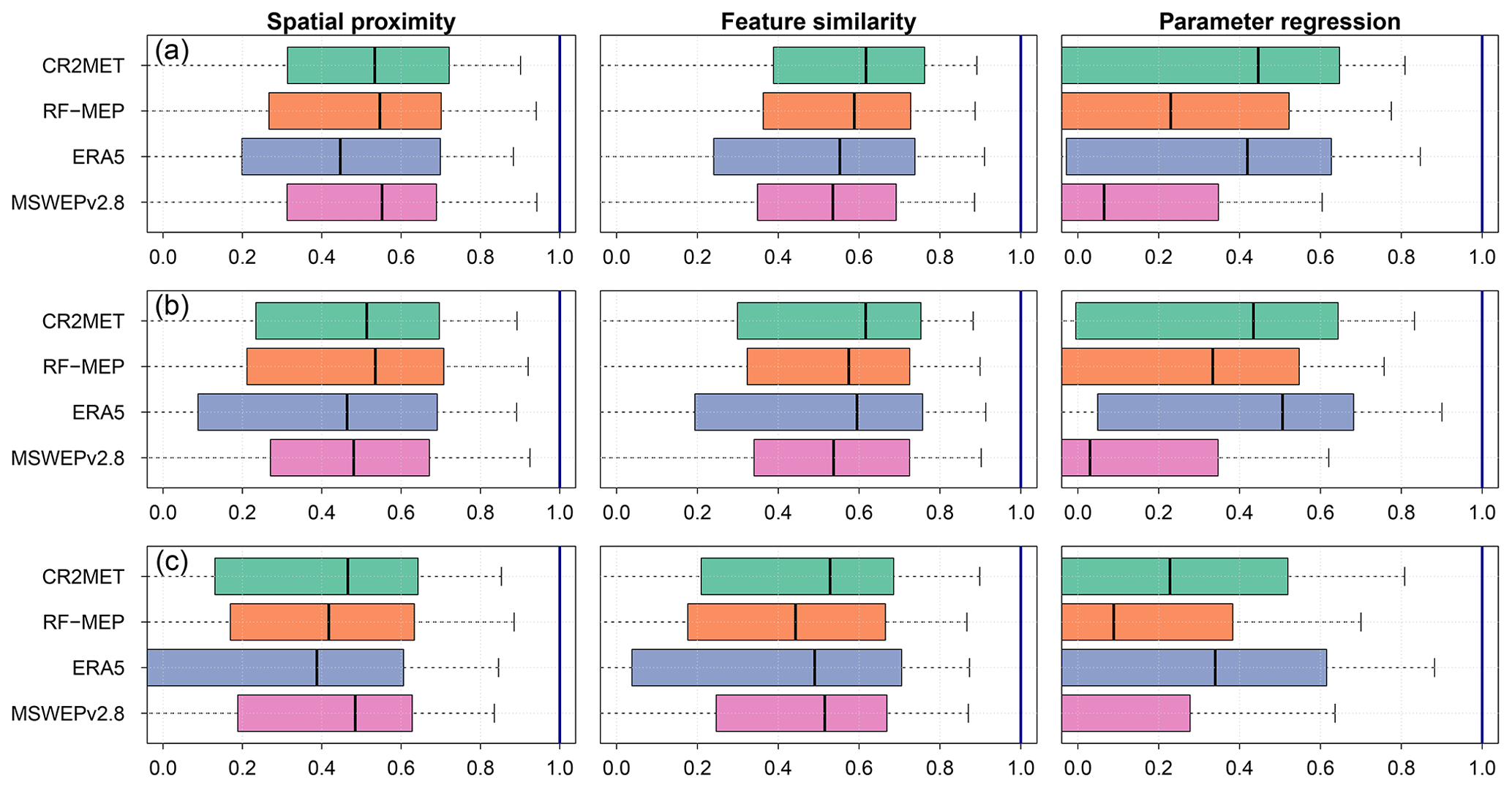
Figure 6 Leave-one-out cross-validation results for the three regionalisation methods applied with different P products during the (a) calibration (2000–2014), (b) Verification 1 (1990–1999), and (c) Verification 2 (2015–2018) periods.

For each regionalisation technique, Fig. 7 summarises the spatial distribution of the performance of each P product for the calibration, Verification 1, and Verification 2 periods. The spatial patterns obtained for all regionalisation methods were similar, independent of the P product or the evaluated period, except for parameter regression, which yielded poor results over high-elevation catchments and under dry conditions (Verification 2). These results indicate that spatial proximity and feature similarity present very similar spatial performance patterns, with feature similarity yielding higher KGE^′ values over the three evaluated periods.

All P products performed better in the Central Chile and South regions than in the Far North, Near North, and Far South regions. The low performance of regionalisation in the arid north is very likely due to the convective nature of storms occurring in the highlands of the Chilean Altiplano (elevations above 4000 m a.s.l.) and the low density of Q stations over this area. Despite this general low performance, RF-MEP was the best-performing P product over the Far North region for both spatial proximity (median KGE^′ of 0.28) and feature similarity (median KGE^′ of 0.46) in the calibration period, suggesting that merging P products and ground-based observations helps to improve, to some extent, the performance of hydrological modelling across arid regions. Conversely, all products outperformed RF-MEP over the Far South. Figure 7 also highlights that spatial proximity provides the best performance over the Far South, with median KGE^′ values higher than 0.46, 0.27, 0.30, and 0.35 for CR2MET, RF-MEP, ERA5, and MSWEPv2.8, respectively. The systematic lower performance of feature similarity compared to spatial proximity over the Far South (except for the case of ERA5) could be attributed to (i) the lack of catchment characteristics that represent the hydrological behaviour of this complex area dominated by polar and temperate climates and (ii) the low number of potential donor catchments (11 for latitudes >49^∘ S), combined with their varied hydrological regimes. For the most southern catchments, the highest P intensities occur during March–May, while the lowest P occurs between June–August, which differs from catchments throughout the rest of the country (Alvarez-Garreton et al., 2018, their Fig. 9). This may affect the hydrological simulations when model parameters from catchments located <49^∘ S are transferred to these far southern catchments.

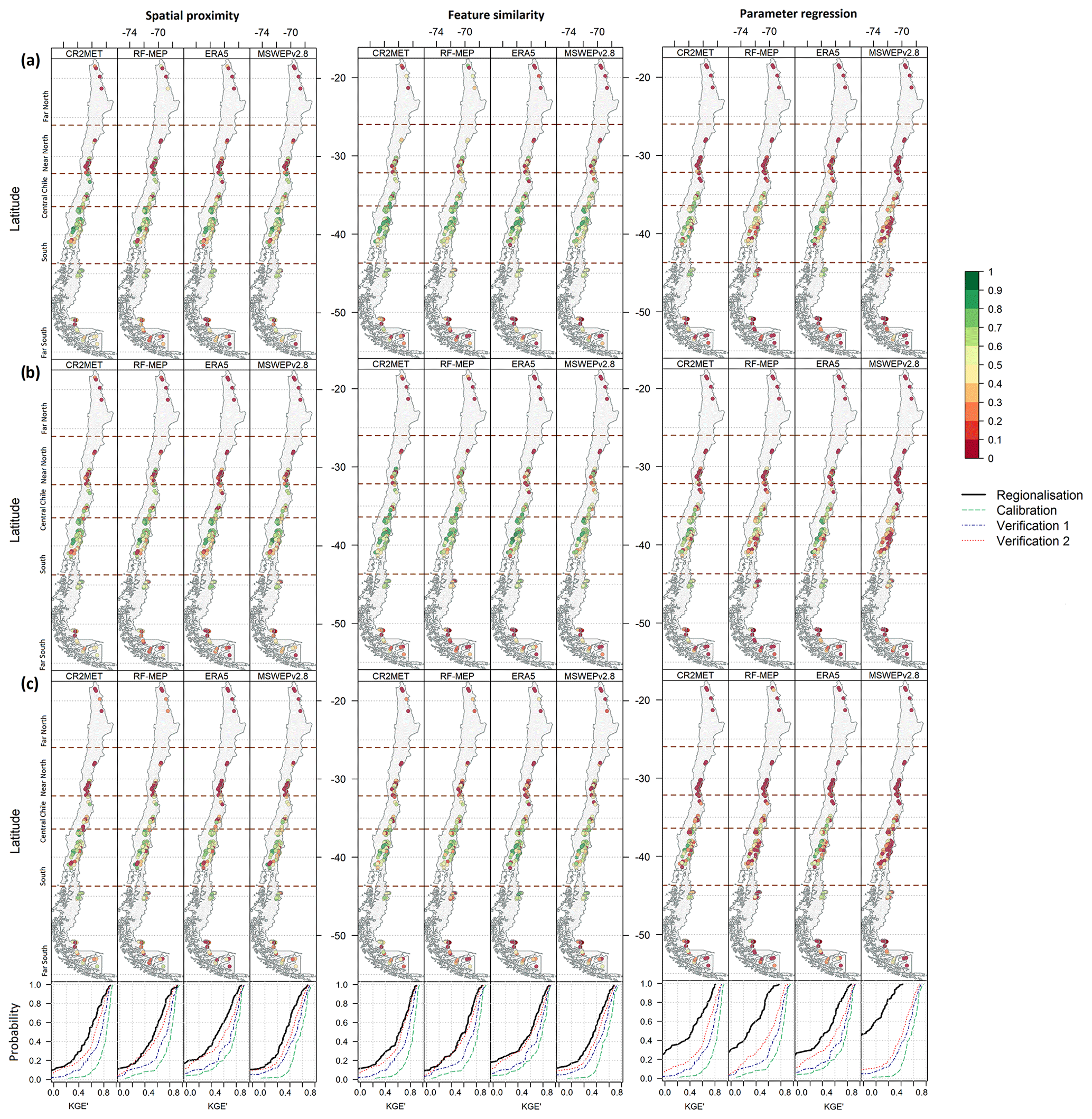
Figure 7 Spatial performance of the leave-one-out cross-validation results for the three regionalisation methods according to P products used to force TUWmodel. Results are presented for the (a) calibration (2000–2014), (b) Verification 1 (1990–1999), and (c) Verification 2 (2015–2018) periods. The panels beneath the map plots refer to the ECDFs of the corresponding regionalisation technique for the entire period of analysis (1990–2018) and P products (black) against the performances during the independent calibration (green), Verification 1 (blue), and Verification 2 (red) periods.

4.2 Evaluation of regionalisation techniques

4.2.1 Overall performance

For each P product, Fig. 8 compares the performances of the three regionalisation techniques with those obtained in the independent calibration and verification periods. The independent calibration of each catchment represents the highest model performance that can be obtained for a specific combination of hydrological model, objective function, and catchment (i.e. an absolute benchmark), whereas the two verification periods were used to evaluate the performance of the regionalisation techniques over independent time periods (i.e. as verification benchmarks). There are marked differences in performance according to the P product used to force the TUWmodel, regardless of the regionalisation method and the evaluated period. For example, ERA5 has more dispersion in the KGE^′ values compared to other products for the cases of feature similarity and spatial proximity, while for parameter regression, it tends to perform the best. For all P products and evaluation periods, feature similarity performed the best, followed by spatial proximity and parameter regression, which is consistent with results from multiple studies (e.g. Parajka et al., 2005; Oudin et al., 2008; Bao et al., 2012; Garambois et al., 2015; Neri et al., 2020). Parameter regression had both the lowest median KGE^′s as well as the largest spread. Comparing the two verification periods, results obtained during the (near-normal/wet) Verification 1 period were close to those obtained during calibration, while those obtained during the (dry) Verification 2 period were substantially lower, especially for spatial proximity and parameter regression.

These results are in agreement with the lower panels located below each map in Fig. 7, which show the empirical cumulative distribution functions (ECDFs) of the performance of each regionalisation technique during the complete period of analysis (1990–2018). These ECDFs compare the relative performance of each regionalisation method against those obtained from the independent calibration and verification of each catchment (used as benchmarks). As expected, all regionalisation methods presented a lower performance than the independent calibration and verification, with this reduction more pronounced for parameter regression.

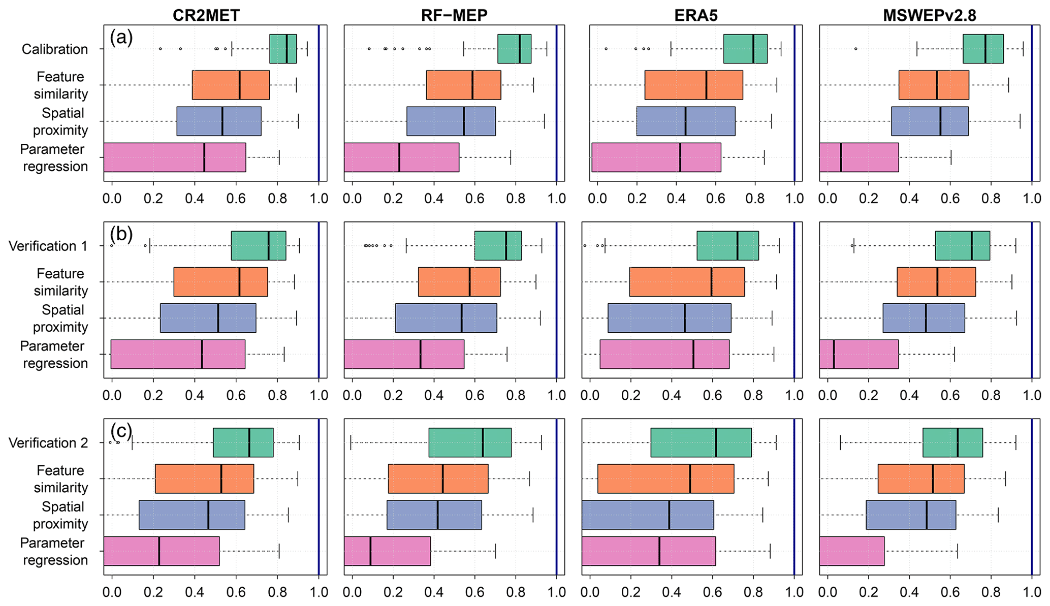
Figure 8 Performance of the regionalisation methods during the (a) calibration (2000–2014), (b) Verification 1 (1990–1999), and (c) Verification 2 (2015–2018) periods.

4.2.2 Impact of hydrological regimes

Figure 9 shows the performance of the regionalisation techniques according to hydrological regime for all P products during the calibration period (and Figs. S9 and S10 of the Supplement show the same for the two verification periods). Feature similarity provided the best median performance for all hydrological regimes and P products except for snow-dominated catchments, where spatial proximity performed the best for MSWEPv2.8 for calibration and Verification 2. These results demonstrate that there was no single P product that outperformed the others for all regionalisation techniques and hydrological regimes. In other words, the best-performing P product depends on the hydrological regime and chosen regionalisation method for our case study. For feature similarity in snow-dominated catchments, RF-MEP performed the best for calibration and Verification 1, while CR2MET performed the best during Verification 2. For nivo-pluvial catchments, CR2MET provided the best performance during calibration and Verification 1, while MSWEPv2.8 performed the best during Verification 2. CR2MET and ERA5 performed the best in pluvio-nival catchments for the case of feature similarity, while all products performed similarly for spatial proximity. Finally, ERA5 performed the best for feature similarity in all periods across the rain-dominated catchments.

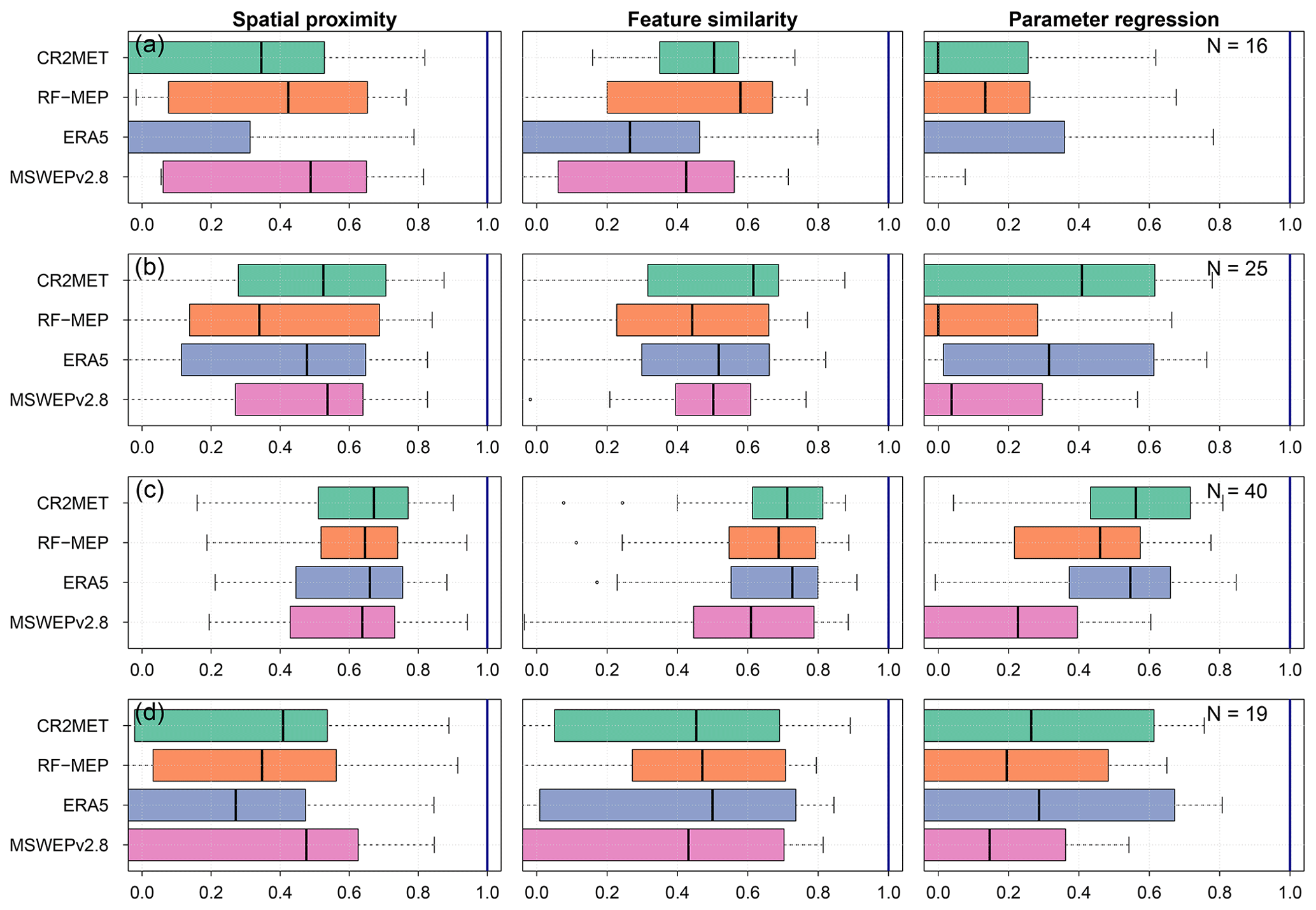
Figure 9 Performance of regionalisation methods for calibration (2000–2014) according to the hydrological regime: (a) snow-dominated, (b) nivo-pluvial, (c) pluvio-nival, and (d) rain-dominated. N denotes the number of catchments per hydrological regime.

4.3 Impact of nested catchments

We evaluated the influence of the nested catchments on the regionalisation results. Figure 10 shows the performance of the three regionalisation methods for the subset of 56 nested catchments that share a common area with at least one other catchment (i.e. the 42 nested catchments as well as all corresponding parent catchments). Here, we compare the regionalisation performance using all potential donors (dark colours) with the performance when excluding nested catchments as potential donors (light colours). The order of performance of the regionalisation methods and P products did not vary when the nested catchments were excluded, as feature similarity and CR2MET remained the best-performing method and product, respectively. As expected, the regionalisation technique with the largest reduction in performance when excluding nested catchments was spatial proximity, followed closely by feature similarity. All P products showed a slight performance reduction and increased dispersion for spatial proximity, except for MSWEPv2.8, which showed a slight increase in the KGE^′ median value. Feature similarity showed a slight reduction in performance when the nested catchments were excluded; however, the median values remained almost the same. The change in performance of parameter regression was negligible after the exclusion of nested catchments because, in the particular case of Chile, excluding only a few catchments had a negligible effect on the non-linear relationships between model parameters and the selected climatic and physiographic characteristics (see Table 4).

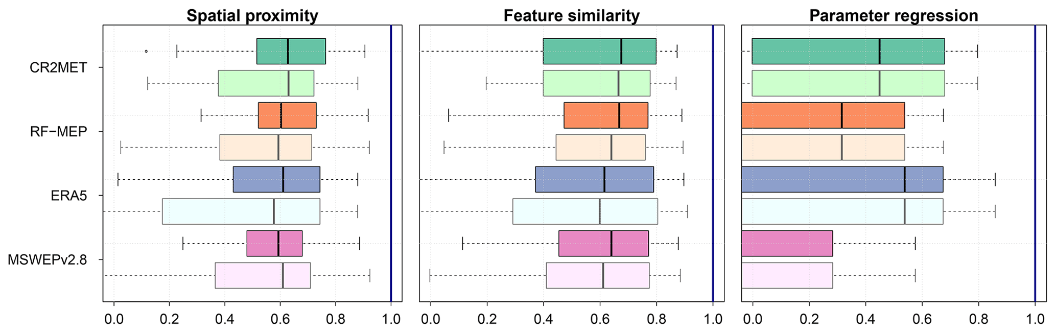
Figure 10 Comparison of regionalisation performance using all catchments as potential donors (dark colours) against the performance when nested catchments are excluded as potential donors (light colours).

4.4 Impact of the number of donors in feature similarity

Figure 11 shows the performance of feature similarity during the calibration and both verification periods when varying the number of donors used to transfer model parameters to ungauged catchments (see Sect. 3.6). In general, the highest median performance is obtained when using four or more donor catchments. However, the application of a t test demonstrated that the improvement in the KGE^′ values obtained when increasing to more than one donor was not statistically significant. The results show that the performance varies according to the P product and selected period of analysis. For the calibration period, feature similarity produced similar median values to those obtained with spatial proximity when one donor was used, while the performance improved as more donors were included. For both verification periods, feature similarity (median KGE^′ values from 0.44 to 0.64) outperformed spatial proximity (median KGE^′ values ranging from 0.39 to 0.54). For all three periods, feature similarity provided better performance considering the distribution of the KGE^′ values.

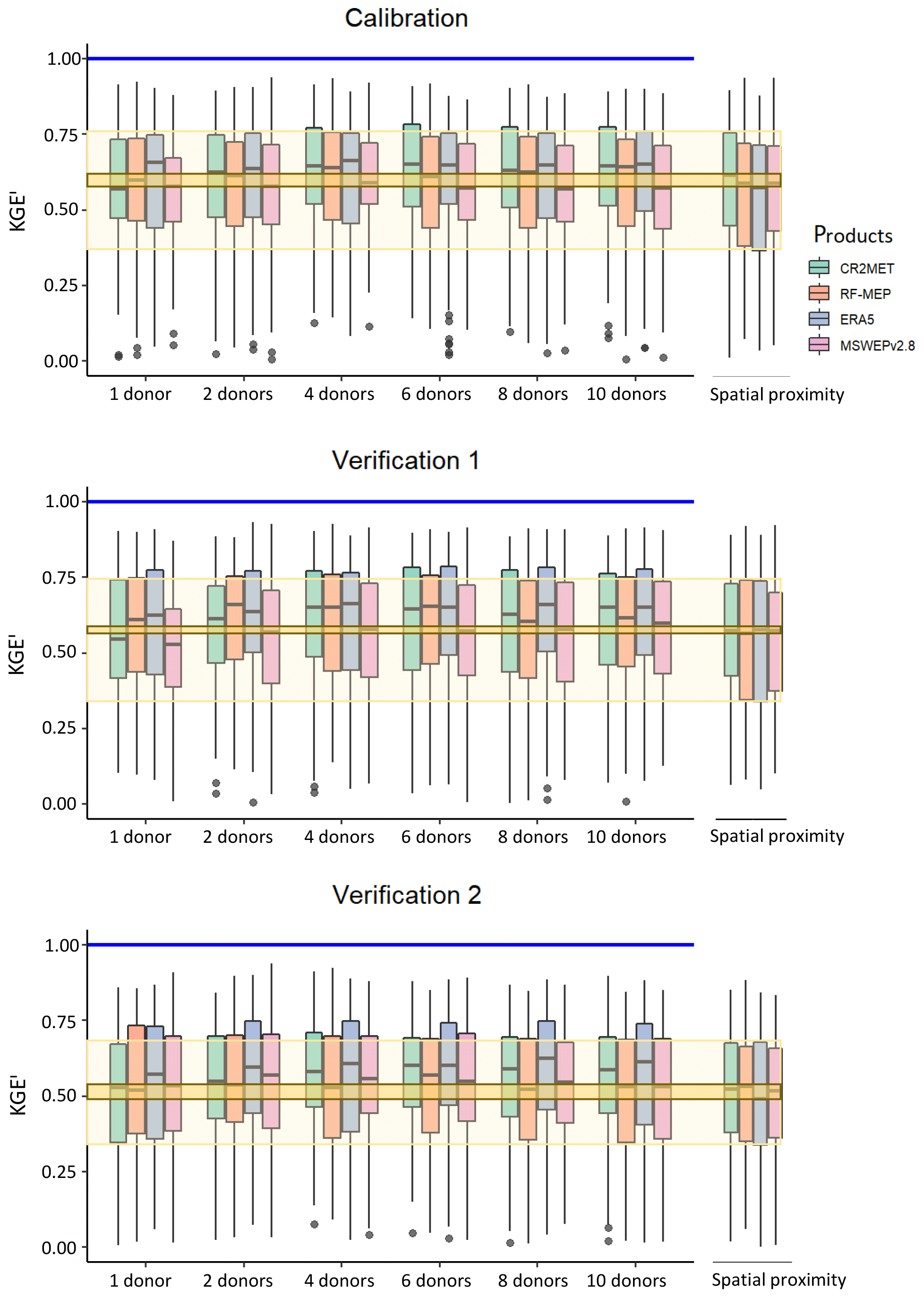
Figure 11 Influence of the number of donors used for feature similarity for calibration (2000–2014), Verification 1 (1990–1999), and Verification 2 (2015–2018). The results from spatial proximity are included on the right of each panel for comparison purposes. The dark yellow box denotes the upper and lower bounds of the median performance (of the four P products) obtained with spatial proximity, the lighter yellow box represents the upper and lower bounds of the interquartile range for spatial proximity, and the blue lines represent the optimum KGE^′ value.

5 Discussion

5.1 Performance of P products

During the independent catchment calibration (2000–2014) and two verification periods (1990–1999 and 2015–2018), good performances were obtained with all P products (see Fig. 4). When decomposing the results of the KGE^′ objective function into its three components (see Appendix C), r exhibited the lowest performance, while β and γ values were generally closer to their optimal values, particularly for calibration and Verification 1. The results obtained with ERA5, which is a reanalysis product, were as good or even better than those obtained with the gauge-corrected products CR2MET, RF-MEP, and MSWEPv2.8 (e.g. see results for the pluvio-nival catchments in Fig. 5). This is in agreement with Tarek et al. (2020), who concluded that ERA5 should be considered a high-potential dataset for hydrological modelling in data-scarce regions. The good performance of ERA5 suggests that, for the particular case of Chile, merging P products with ground-based measurements does not necessarily translate into improved hydrological model performance, which may be attributed to (i) the lack of P rain gauges in the Andes Mountains; (ii) the ability of the rainfall-runoff model to compensate for the P forcing (visible in the performances of the β and γ components, Appendix C), and (iii) the fact that P products still have errors in the detection of P events that could impact the representation of the modelled Q dynamics (as suggested by the relative lower performance of the r component of the KGE^′).

Furthermore, the similar performances obtained with uncorrected (ERA5) and gauge-corrected (CR2MET, RF-MEP, and MSWEPv2.8) P products, both in wet and dry periods, highlight that there was no single P dataset outperforming the others in all periods. These results demonstrate that the calibration of hydrological model parameters smooths out, to some extent, the spatio-temporal differences between P products (see Figs. 2, 3, 6 and 9), which is in agreement with previous studies that have demonstrated that model calibration with each P product improves the performance of Q simulations (e.g. Artan et al., 2007; Stisen and Sandholt, 2010; Bitew et al., 2012; Thiemig et al., 2013). The decomposition of the KGE^′ into its components also demonstrated the ability of the TUWmodel to compensate for the total volume of P, as the β component was close to the optimum value, particularly for calibration and Verification 1 (see Appendix C), which can be attributed to the improved detection of P events of the merged products (regarding RF-MEP, see Baez-Villanueva et al., 2020). This can also be observed for MSWEPv2.8, as it produced the best performance over snow-dominated catchments under dry conditions (Verification 2).

Regarding the suitability of P products for parameter regionalisation, RF-MEP provided slightly better results in the Far North for the calibration period using both spatial proximity and feature similarity, suggesting that P products that are merged with ground-based information over arid climates can improve regionalisation performance. The lower performance obtained in regionalisation with ERA5 in the Far North compared to the other P products (median values <0.18 for feature similarity in all periods) can be attributed to its high P values, which are likely due to the lack of ground-based P stations over Chile in the development of the product. The incorporation of ground-based stations has the potential to (i) compensate for overestimations caused by the evaporation of hydrometeors before they reach the ground (Maggioni and Massari, 2018) and (ii) improve event-based detection skills (Baez-Villanueva et al., 2020; Zhang et al., 2021). The latter is evident in CR2MET and MSWEPv2.8, which are both based on ERA5 but included several rain gauges in the Far North and have a higher performance than ERA5 (see Figs. 2, 3, and S1).

Despite the low performance of all P products in the Far North and Near North (median KGE^′ values <0.58; see Fig. 7), the TUWmodel appears to be flexible enough to compensate, to some extent, for differences between P products. A similar conclusion was obtained by Elsner et al. (2014), who examined differences between four meteorological forcing datasets and their implications in hydrological model calibration in the western United States using the variable infiltration capacity model (VIC; Liang et al., 1994). Our results are also in agreement with Bisselink et al. (2016), who concluded that parameter sets obtained during calibration partially compensated for the bias of seven P products used to force the fully distributed LISFLOOD model in four catchments in southern Africa.

An unexpected result from this study is that the spatial resolution of the P products did not play a major role in model performance during calibration, verification and regionalisation; although CR2MET and RF-MEP have a higher spatial resolution (0.05^∘; ∼25 km²) than MSWEPv2.8 (∼ 0.10^∘; ∼100 km²) and ERA5 (∼0.28^∘; ∼625 km²), all four products performed well during the independent calibration of the hydrological model and the two verification periods. The performance of ERA5 over the 25 smallest catchments during regionalisation (area <353.1 km²) was similar to that obtained with products with a higher spatial resolution (Fig. S11 of the Supplement). This can be attributed to the fact that Chile is dominated by large-scale frontal systems (Zhang and Wang, 2021); and therefore, coarse-resolution products may perform well over small catchments. Our results also align with the findings of Maggioni et al. (2013), who concluded that the loss of spatial information associated with coarser resolution (e.g. ERA5) can be compensated for through model calibration.

5.2 How does the calibration of the TUWmodel compensate for differences in P?

The calibration of TUWmodel was able to compensate, to some extent, for differences in annual and intra-annual P amounts, intermittency, and extremes (see Figs. 2 and 3) among the four products. Using the example of the nivo-pluvial catchments, Fig. 12 illustrates how TUWmodel parameters compensate for differences between the P forcings used in calibration, while Fig. 13 shows the corresponding variations in the mean monthly water balance components. Similar figures for snow-dominated, pluvio-nival, and rain-dominated catchments can be found in the Supplement (Figs. S12–S17).

In general, the calibrated parameters behave as expected for each hydrological regime. A notable exception is ERA5, which shows low values for the snow correction factor (SCF) in nivo-pluvial and snow-dominated catchments (Figs. 12 and S12). These catchments are primarily located in the arid Near North region (see Fig. 2 and Figure S15), where the estimated winter P is substantially lower for CR2MET, RF-MEP, and MSWEPv2.8, and a high SCF corrects this apparent underestimation. The lower P amounts presented in these products may reflect the incorporation of information from rain gauges located in drier, low-lying areas to correct their P estimates (see Fig. S1).

ERA5 presented relatively low SCF values over nivo-pluvial catchments compared to the other P products (Fig. 13), which is expected because it exhibits the highest P values. Conversely, because RF-MEP has the lowest mean monthly P over the nivo-pluvial catchments, the model adjusts the evaporation, snow water equivalent, and soil moisture components (Fig. 13), thus increasing the simulated Q (to match the observed Q). Substantial differences were obtained for LPrat and field capacity (FC), which directly affect evaporation and soil moisture. For example, over the nivo-pluvial catchments, the LPrat and FC values for RF-MEP are similar to those of ERA5, despite RF-MEP having substantially lower P amounts, which in turn is reflected in the reduced soil moisture and evaporation amounts. The differences between LPrat and FC according to P product are even more pronounced for snow-dominated catchments (Fig. S12).

Finally, higher values of the nonlinear parameter for runoff production Beta reduce the amount of water that leaves the catchment as runoff (Széles et al., 2020, their Eq. 7). For all hydrological regimes except pluvio-nival, the median Beta parameter is substantially higher for ERA5 than for the other P products. The larger Beta values obtained with ERA5 are expected to attenuate the runoff generation from extreme P events (see Fig. 3c and d). Interestingly, the Beta parameter is zero in some pluvio-nival catchments, which means that all liquid P and snowmelt was used to generate runoff (Fig. S16). This behaviour was more pronounced with RF-MEP and MSWEPv2.8, which exhibited the lowest P amounts and longer dry spells (Fig. 3a) over these catchments. In general, the storage components obtained from each P product (computed as the sum of the two deepest reservoirs of the model; see Széles et al., 2020, their Fig. 3) are similar for all four P products.

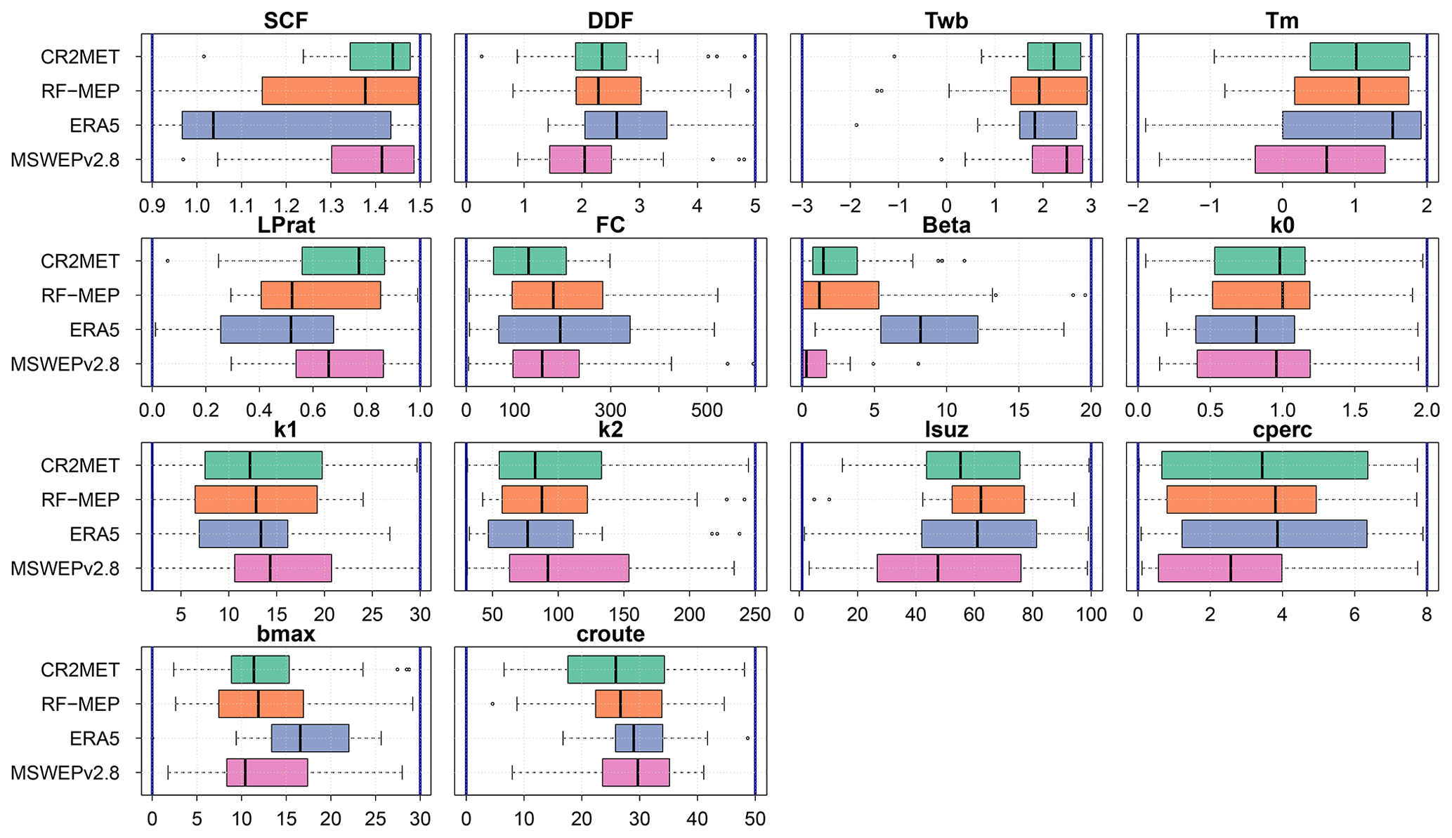
Figure 12 Model parameters obtained through calibration in nivo-pluvial catchments. The vertical blue lines indicate the upper and lower limits of the parameter ranges.

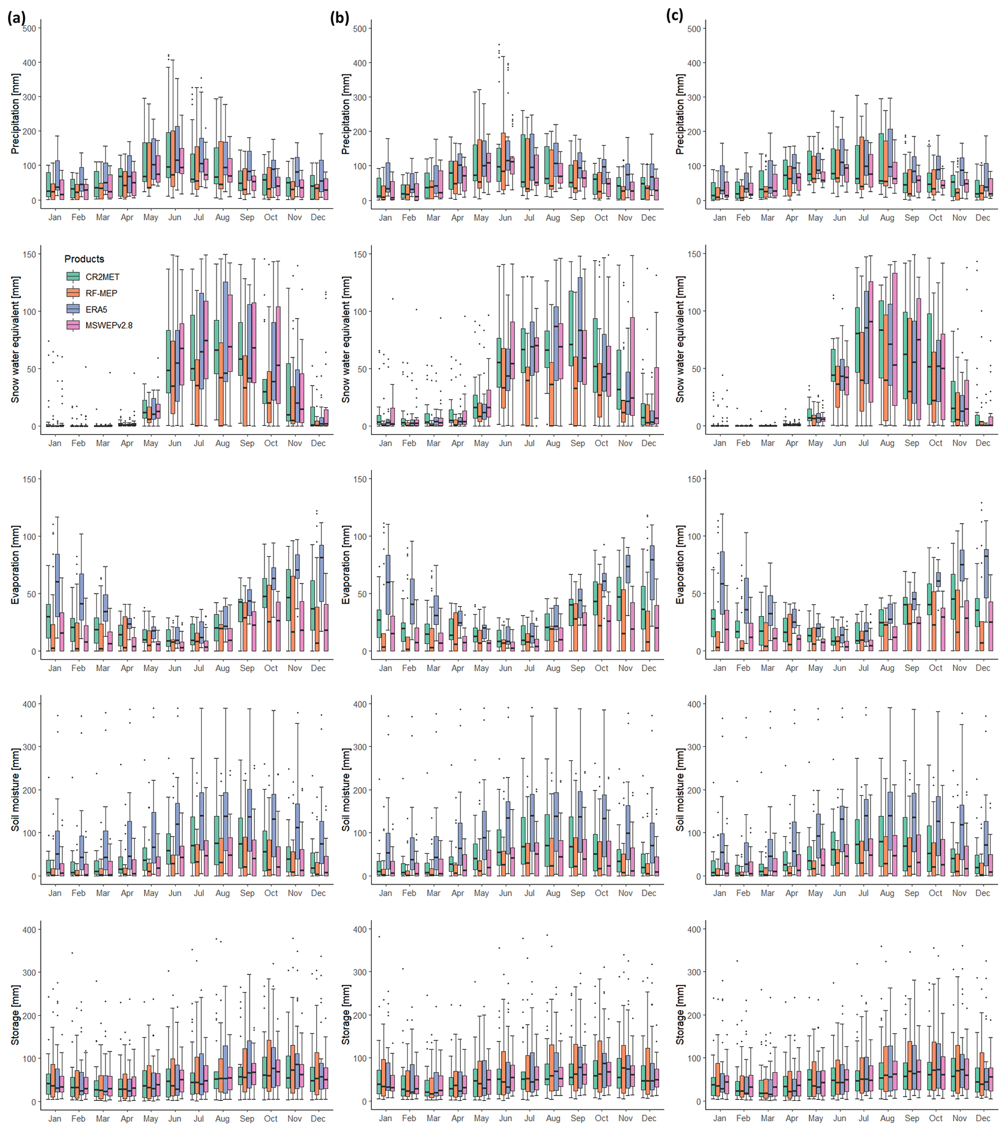
Figure 13 Mean monthly water balance components over nivo-pluvial catchments, obtained by forcing the TUW model with different P products for the (a) calibration (2000–2014), (b) Verification 1 (1990–1999), and (c) Verification 2 (2015–2018) periods. Mean monthly P was added for comparison purposes.

5.3 Evaluation of regionalisation techniques

The compensation due to the flexibility of the TUWmodel observed during the independent calibration and verification (see Sect. 5.2) also influences the regionalisation performance. Feature similarity provided the best performance when the TUWmodel was forced with all P products (Fig. 8), while spatial proximity provided similar performance to feature similarity over the Central Chile and South regions, where there is a high density of Q stations. These results are in agreement with Parajka et al. (2005), Oudin et al. (2008), and Neri et al. (2020), who demonstrated that spatial proximity performs well over densely gauged regions.

The inclusion of donor catchments with low model performance introduces a diversity that has the potential to benefit Q prediction in ungauged catchments, as discussed by Oudin et al. (2008). We decided to incorporate these catchments in the regionalisation process because of the diversity of climates and physiographic characteristics across continental Chile (see Fig. 1), with the potential downside that this may lead to errors in the transferred model parameters. Additionally, the similarity between the performance of spatial proximity and feature similarity can be partially attributed to the fact that six of the nine selected catchment characteristics are directly or indirectly related to climate, which in Chile is highly related to the geographical locations of the catchments. Parameter regression was the regionalisation method that provided the worst results (Figs. 6 and 8); however, Fig. 7 shows that this method generated good results over low-elevated areas of the Central Chile and South regions, where there are many potential donor catchments located nearby.

The compensation for P differences obtained through model calibration also affected the relative performance of regionalisation techniques, producing unrealistic parameter sets in some donor catchments. In particular, such compensation may have impacted the spatial transferability of model parameters with the parameter regression method. The main reason for this is that, unlike techniques that transfer the entire parameter sets, the regression process denatures the already uncertain model parameters by applying independent regression procedures using climate and physiographic characteristics (Arsenault and Brissette, 2014). This challenge can be overcome by simultaneously optimising both the model parameters and the regression equations (e.g. Samaniego et al., 2010; Rakovec et al., 2016; Beck et al., 2020a), but such an exercise is outside of the scope of this study.

For both spatial proximity and feature similarity, the best and worst results were obtained for pluvio-nival catchments and rain-dominated catchments, respectively. Figure 9 shows the performances of the three regionalisation techniques according to hydrological regimes (see Fig. 1d) for the calibration period. Comparing Figs. 5 and 9, it is evident that the snow-dominated catchments performed substantially worse than in the independent performance during the same period (Fig. 5). On the other hand, the pluvio-nival catchments performed systematically better in the independent calibration and verification as well as in regionalisation. This could be attributed to (i) the ability of the model to reproduce Q in this regime and (ii) the increased likelihood of transferring model parameters from a catchment with the same hydrological regime, as they are grouped closed together and form 40 % of the total number of catchments.

5.4 Impact of nested catchments

Nested catchments play an important role in the performance of regionalisation methods as they are more likely to have a strong climatological and physiological similarity to each other. As observed in Fig. 10, the regionalisation method that was most impacted by the exclusion of nested catchments was spatial proximity, followed by feature similarity. These results are in agreement with previous studies, where the exclusion of nested catchments reduced the performance of regionalisation techniques (Merz and Blöschl, 2004; Oudin et al., 2008; Neri et al., 2020). Feature similarity only presented a slight decrease when the nested catchments were neglected, which can be attributed to the low degree of nestedness (i.e. the number of catchments that are nested in a larger one). As expected, the exclusion of nested catchments had a negligible effect on parameter regression, as the removal of relatively few catchments had a negligible impact on the non-linear relationships between the climatic and physiographic characteristics and the model parameters that were determined using all potential donor catchments. The reduction of regionalisation performance when the nested catchments were removed was lower than the reduction reported in a case study over Austria (Neri et al., 2020, their Figure 9a), which could be attributed to (i) the degree of nestedness, as the unique geography of Chile limits, to some extent, the number of nested catchments within any larger catchment (only 10 of the 100 selected catchments contained more than three nested catchments); and (ii) the percentage of catchments that are nested (42 % in this study, compared to 65 % in the Austrian case study).

5.5 Impact of number of donor catchments

Increasing the number of donor catchments in feature similarity improved the regionalisation performance. This is in agreement with several studies that have demonstrated that using an ensemble of multiple donor catchments improves regionalisation results (McIntyre et al., 2005; Zelelew and Alfredsen, 2014; Garambois et al., 2015; Beck et al., 2016; Neri et al., 2020). Figure 11 shows that there is a slight increase in performance when four donors or more are used, independent of the P product and evaluated period. These results are similar to those of Neri et al. (2020), who determined that three donors were optimal for the TUWmodel over Austrian catchments. Feature similarity still outperformed spatial proximity when only one catchment was used to transfer the model parameters to the ungauged catchments, which is in agreement with multiple studies that have shown the ability of this method to produce good regionalisation results (Parajka et al., 2005; Oudin et al., 2008; Bao et al., 2012; Garambois et al., 2015; Neri et al., 2020).

6 Conclusion

Accurate streamflow predictions in ungauged catchments are critical for water resources management, and their generation is challenged by uncertainties arising from P products. In this paper, we assessed the relative performance of three common regionalisation techniques (spatial proximity, feature similarity, and parameter regression) over 100 near-natural catchments located in the topographically and climatologically diverse Chilean territory. Four P products (CR2MET, RF-MEP, ERA5, and MSWEPv2.8) were used to force the semi-distributed TUWmodel at the daily timescale, using the KGE^′ as the calibration objective function and metric to assess (i) the impact of selecting different P forcings on the relative performance of regionalisation techniques and (ii) possible connections between regionalisation performance and hydrological regimes. Our key findings are as follows:

1. For the selected P products, the one that provided the best (worst) performance during independent calibration and verification did not necessarily yield the best (worst) results during regionalisation.

2. The P products corrected with daily ground-based measurements did not necessarily yield the best hydrological model performance. However, we expect that P products with lower performances than the ones used in this study might benefit from such a correction.

3. The spatial resolution of the P products did not noticeably affect model performance during the calibration and verification periods.

4. The TUWmodel was able to compensate, to some extent, the differences between P products through model calibration by adjusting the model parameters and, therefore, adjusting the water balance components (e.g. snow water equivalent, evaporation, and soil moisture).

5. Feature similarity was the best-performing regionalisation technique, regardless of the choice of gridded P product or hydrological regime.

6. Spatial proximity was the second best-performing regionalisation method because, in our study area, spatial proximity is a good proxy for climatic similarity for most neighbouring catchments.

7. Parameter regression provided the worst regionalisation performance, reinforcing the importance of transferring complete parameter sets to ungauged catchments.

8. The performance of regionalisation techniques can depend on the hydrological regime. We obtained the best results in pluvio-nival catchments with spatial proximity and feature similarity, while the same techniques provided the worst performance in rain-dominated catchments.

9. The exclusion of (relatively few) nested catchments had a minimal impact on the non-linear relationships between the climatic and physiographic characteristics (i.e. predictors) and model parameters (i.e. predictands), having a negligible effect on parameter regression results.

10. The performance of feature similarity increased when four or more catchments were used as donors; however, the differences in performance were not statistically significant when compared to the results of using only one donor.

The results presented here are valid only for near-natural catchments across continental Chile. Nevertheless, they provide guidance for ongoing and future studies involving the application of gridded P products for regionalising hydrological model parameters in ungauged basins. The feature similarity procedure described here could be used to refine the parameter regionalisation approach adopted for national-scale hydrological characterisations in Chile (e.g. Bambach et al., 2018; Lagos et al., 2019). Additionally, further analyses could address (i) the effects that objective functions may have on the simulation of streamflow-derived hydrological signatures (e.g. Pool et al., 2017); (ii) other states and fluxes derived from remote sensing data (e.g. Dembélé et al., 2020); (iii) the influence of parameter equifinality (mainly for parameter regression), which can be accounted for by simultaneously optimising the model parameters and the regression equations, as described in Beck et al. (2020a); (iv) the use of additional model structures, implemented through flexible modelling platforms (e.g. Clark et al., 2008; Knoben et al., 2019); and (v) the sensitivity of regionalisation results with respect to modified climate scenarios.

Appendix A: Conceptual figure of hydrological regimes

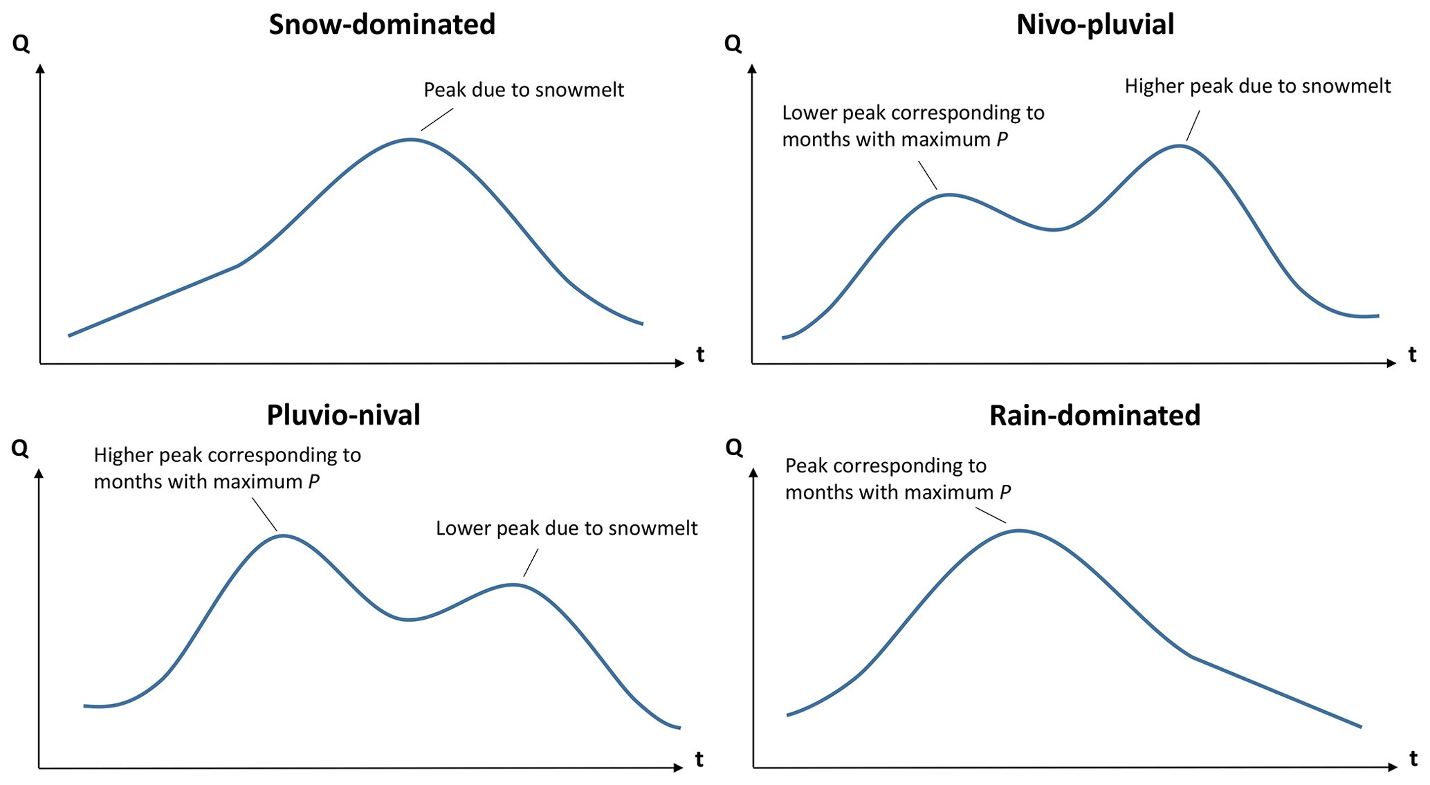
Figure A1 Conceptual illustration of the hydrological regimes used to classify the 100 near-natural catchments used in this study.

Appendix B: Selection of catchment characteristics for feature similarity

To avoid including redundant information when quantifying catchment similarity, we examined the correlations between the catchment characteristics described in Table 4. Figure B1 shows correlation matrices between catchment characteristics using the Pearson correlation (a) and the Spearman rank (b) correlation coefficients. We only present correlations obtained with CR2MET, since very similar results were obtained with the remaining P products. Because the mean and median elevation are highly correlated (values of 1.0 and 0.99 for the Pearson and Spearman correlation coefficients, respectively), we decided to keep the median elevation under the assumption that it is more representative of topographic conditions, given the pronounced elevation gradients in continental Chile. Similarly, mean annual PE was excluded because of its high correlation with mean annual T (0.87 and 0.86 for the Pearson and Spearman correlation coefficients, respectively), notwithstanding that T was used to calculate PE. SDII was also excluded due to its high correlation to the Rx5day (0.97 for both coefficients). Finally, we excluded the snow cover from CAMELS-CL, as we found it to be unreliable over the snow-dominated catchments selected in our analysis.

Figure B1 Correlation matrices of the catchment characteristics described in Table 4 using CR2MET as the P product for (a) the Pearson correlation, to evaluate linear correlation, and (b) the Spearman correlation, to evaluate the monotonic correlation.

Appendix C: Performance of the components of the KGE^′

Table C1 Quantiles 0.25 and 0.75 of the correlation coefficient (r) of the KGE^′ over the selected catchments.

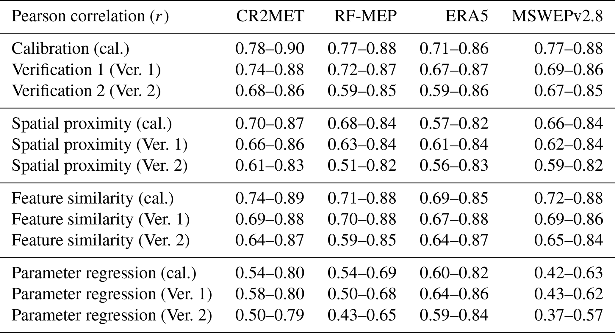
Table C2 Quantiles 0.25 and 0.75 of the bias ratio (β) of the KGE^′ over the selected catchments.

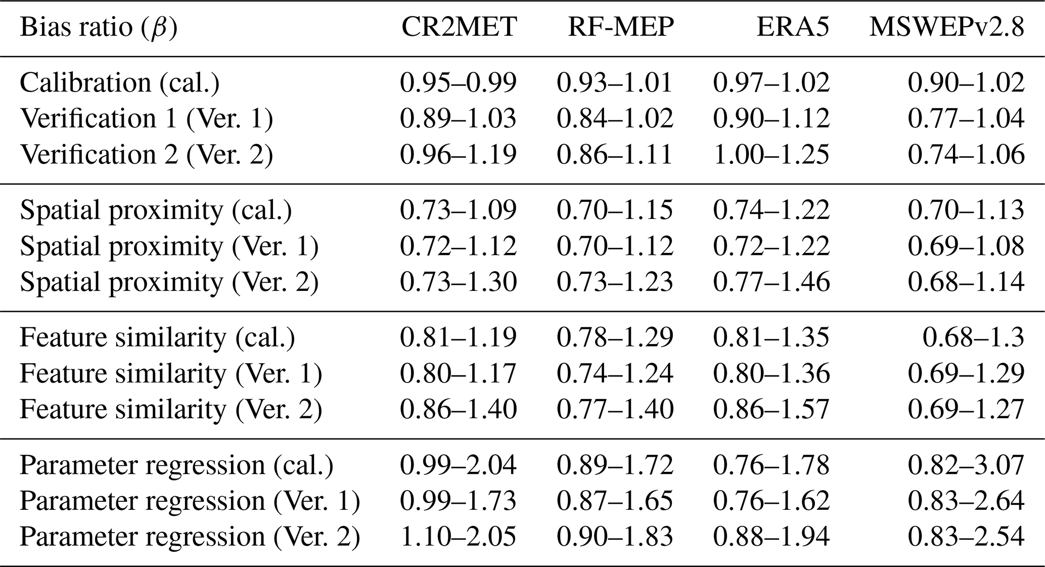
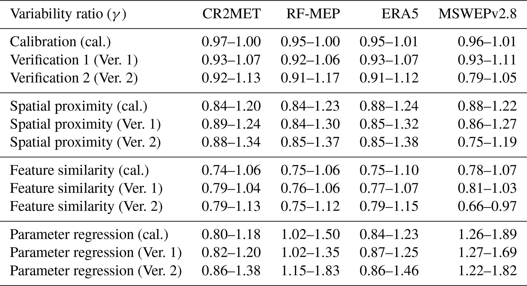
Table C3 Quantiles 0.25 and 0.75 of the variability ratio (γ) of the KGE^′ over the selected catchments.