the Creative Commons Attribution 4.0 License.
the Creative Commons Attribution 4.0 License.
 | 15 Oct 2021
Unshielded precipitation gauge collection efficiency with wind speed and hydrometeor fall velocity
Michael E. Earle
Paul I. Joe
Pierre E. Sullivan
Collection efficiency transfer functions that compensate for wind-induced collection loss are presented and evaluated for unshielded precipitation gauges. Three novel transfer functions with wind speed and precipitation fall velocity dependence are developed, including a function from computational fluid dynamics modelling (CFD), an experimental fall velocity threshold function (HE1), and an experimental linear fall velocity dependence function (HE2). These functions are evaluated alongside universal (KUniversal) and climate-specific (KCARE) transfer functions with wind speed and temperature dependence. Transfer function performance is assessed using 30 min precipitation event accumulations reported by unshielded and shielded Geonor T-200B3 precipitation gauges over two winter seasons. The latter gauge was installed in a Double Fence Automated Reference (DFAR) configuration. Estimates of fall velocity were provided by the Precipitation Occurrence Sensor System (POSS). The CFD function reduced the RMSE (0.08 mm) relative to KUniversal (0.20 mm), KCARE (0.13 mm), and the unadjusted measurements (0.24 mm), with a bias error of 0.011 mm. The HE1 function provided a RMSE of 0.09 mm and bias error of 0.006 mm, capturing the collection efficiency trends for rain and snow well. The HE2 function better captured the overall collection efficiency, including mixed precipitation, resulting in a RMSE of 0.07 mm and bias error of 0.006 mm. These functions are assessed across solid and liquid hydrometeor types and for temperatures between −22 and 19 ∘C. The results demonstrate that transfer functions incorporating hydrometeor fall velocity can dramatically reduce the uncertainty of adjusted precipitation measurements relative to functions based on temperature.
- Article
(3469 KB) - Full-text XML
-
Supplement
(578 KB) - BibTeX
- EndNote


The works published in this journal are distributed under the Creative Commons Attribution 4.0 License. This license does not affect the Crown copyright work, which is re-usable under the Open Government Licence (OGL). The Creative Commons Attribution 4.0 License and the OGL are interoperable and do not conflict with, reduce or limit each other.
© Crown copyright 2021
Automated catchment-type precipitation gauge measurements are critical as references for, and input to, weather, climate, hydrology, transportation, and remote sensing applications. The systematic bias and uncertainty of gauge measurements due to wind-induced undercatch are a major challenge, particularly with respect to the measurement of mixed and solid precipitation (Rasmussen et al., 2012; Kochendorfer et al., 2018). For example, an unshielded weighing precipitation gauge can capture less than 50 % of the actual amount of solid precipitation falling in air when the wind speed exceeds 5 m s−1 (Kochendorfer et al., 2017b). This measurement challenge has prompted (1) modelling studies to better understand and visualize the undercatch of hydrometeors by precipitation gauges and (2) the development of transfer functions to adjust measurements for undercatch effects. Previous work in each of these domains is outlined in Sect. 1.1 and 1.2, respectively. The objectives of the present study, which implements numerical modelling and experimental analysis to develop transfer functions with wind speed and hydrometeor fall velocity dependence, are presented in Sect. 1.3.
1.1 Modelling studies
Computational fluid dynamics (CFD) studies have been used to simulate the airflow around precipitation gauges and the associated collection efficiencies for rain and solid precipitation (Nešpor and Sevruk, 1999; Constantinescu et al., 2007; Colli, 2014; Colli et al., 2014, 2015, 2016a, b; Thériault et al., 2012, 2015; Baghapour and Sullivan, 2017; Baghapour et al., 2017). These studies have demonstrated the influence of wind speed, turbulence, hydrometeor characteristics (size, density, drag, terminal velocity), and gauge and shield geometry on precipitation gauge undercatch. For rainfall, Nešpor and Sevruk (1999) showed increases in wind-induced error for smaller drop sizes with lower terminal velocities, with errors increasing for higher wind speeds. The conversion factor (inverse of integral collection efficiency) varied with the precipitation intensity and rainfall type, which influenced the distribution of hydrometeor sizes and terminal velocities. Thériault et al. (2012) demonstrated similar trends for snowfall, with collection efficiencies varying significantly with the type of solid precipitation and size distribution. Simulated collection efficiencies for wet snow and dry snow hydrometeors captured the general upper and lower bounds of experimental observations, respectively, with the lower collection efficiency for dry snow hydrometeors attributed to their lower terminal velocity and interaction with the local airflow around the gauge.
For a Geonor gauge with a single-Alter shield, Thériault et al. (2012) used a constant drag coefficient hydrometeor tracking model to develop a series of transfer functions based on wind speed for different hydrometeor types. Colli et al. (2015) extended this work to show the influence of different hydrometeor drag models on collection efficiency results. Empirical drag model results (Khvorostyanov and Curry, 2005), based on the relative hydrometeor-to-air velocity over the hydrometeor trajectory, were shown to yield higher collection efficiencies compared with constant drag coefficient results that can overestimate drag values. Colli et al. (2015) developed transfer functions based on wind speed for unshielded and single-Alter-shielded gauges for three specific hydrometeor size distributions. Further studies, using computationally intensive large eddy simulation (LES) models, better resolved the intensity and spatial extent of turbulence around the gauge orifice, which can lead to temporal variations in collection efficiency results (Colli et al., 2016a, b; Baghapour and Sullivan, 2017; Baghapour et al., 2017). The degree of turbulence was found to vary depending on the specific shield configuration and wind speed (Baghapour et al., 2017).
1.2 Transfer functions
Intercomparisons of precipitation gauges have served as the primary mechanism for developing transfer functions. In the 1998 World Meteorological Organization (WMO) Solid Precipitation Measurement Intercomparison, transfer functions were determined experimentally by comparing measurements from different gauges (primarily manual) with those from a manual collector with a Tretyakov shield in the WMO Double Fence Intercomparison Reference (DFIR) configuration (Goodison et al., 1998). Precipitation events were monitored by observers, who reported the amount and type of snow, wind speed, and temperature statistics for each event. Events were defined based on the duration of continuous snowfall when the reference DFIR precipitation accumulation was greater than or equal to 3 mm. Adjustment functions for unshielded gauge collection efficiencies were recommended for snow, mixed precipitation, and rain, based on the wind speed at gauge height (Goodison, 1978; Goodison et al., 1998; Yang et al., 1998). While these adjustments could be applied to manual precipitation accumulation measurements, their application to automated measurements at shorter timescales, and where the precipitation type may not be well defined, presents a significant challenge (Colli, 2014; Colli et al., 2014, 2016a, b; Thériault et al., 2015, 2012).
The WMO commissioned another intercomparison, the Solid Precipitation Intercomparison Experiment (SPICE), to assess various automated technologies for the measurement of precipitation accumulation and snow depth and to recommend automated field reference systems (Nitu et al., 2018). An automated precipitation gauge configured with a single-Alter shield within a DFIR fence was chosen as the field reference configuration for precipitation accumulation; this was referred to as the Double Fence Automated Reference (DFAR) configuration. Transfer functions for unshielded and shielded gauges were derived as an exponential function of wind speed following the approach of Goodison (1978) and using 30 min precipitation events from the SPICE dataset (Kochendorfer et al., 2017a). Separate functions were developed for solid precipitation and mixed precipitation, as defined by air temperature ranges: less than −2 ∘C for solid precipitation and between −2 and 2 ∘C for mixed precipitation.
Using Bayesian analysis of Norwegian measurement data, Wolff et al. (2015) developed a precipitation phase-independent, continuous transfer function with respect to wind speed and air temperature for a single-Alter-shielded Geonor precipitation gauge. A similar, but less complex, function was developed by Kochendorfer et al. (2017a, 2018) using the SPICE dataset, including results from eight measurement sites in Canada, Norway, Finland, Spain, Switzerland, and the USA. The application of this “universal” function to precipitation accumulation measurements from unshielded weighing gauges in SPICE was shown to reduce the overall bias relative to the DFAR; however, reductions in the root mean square error (RMSE) were less significant (Kochendorfer et al., 2017a, b, 2018; Wolff et al., 2015).
When applying universal adjustments with wind speed and air temperature dependence, the errors can vary significantly by site, presumably driven by differences in climatology (Smith et al., 2020; Kochendorfer et al., 2017a). This has motivated further work on climate-specific transfer functions (Koltzow et al., 2020; Smith et al., 2020). Other studies have proposed the use of precipitation intensity for the improved adjustment of solid precipitation (Chubb et al., 2015; Colli et al., 2020). Another potential avenue for reducing errors in adjusted measurements is by improving the ability of transfer functions to distinguish among different precipitation types and their aerodynamic properties (Thériault et al., 2012; Wolff et al., 2015; Nešpor and Sevruk, 1999).
1.3 Objectives
In this work, adjustment functions incorporating hydrometeor fall velocity are developed to reduce the uncertainty (RMSE) in collection efficiency and precipitation accumulation estimates from unshielded Geonor T-200B3 precipitation gauges. The unshielded gauge configuration allows for the assessment of a broader range of collection efficiencies, as the degree of undercatch is generally more pronounced for unshielded gauges relative to shielded configurations. Further, by focussing on the unshielded configuration, no assumptions are required regarding the behaviour of the shield slats and their role in momentum reduction and turbulence generation around the gauge.
A combined modelling and experimental approach is used in this study. In the modelling component, computational fluid dynamics and Lagrangian analysis is used to characterize the gauge collection efficiency dependence explicitly in terms of wind speed and hydrometeor fall velocity and to derive a corresponding transfer function. Details of the modelling work are included in the Supplement. In the experimental component, fall velocity and precipitation type estimates from the Precipitation Occurrence Sensor System (POSS) are used to investigate how the hydrometeor properties influence the relationships among measured catch efficiency, wind speed, and temperature. Two additional transfer functions are derived experimentally with wind speed and fall velocity dependence. These new transfer functions are assessed against transfer functions with dependence on wind speed and air temperature, including one of the universal functions developed by Kochendorfer et al. (2017a) and a climate-specific function derived herein using a similar methodology.
2.1 CFD model
A computational fluid dynamics model was used to characterize the collection efficiency dependence with wind speed and hydrometeor fall velocity. The model is detailed in the Supplement (Sect. S1.1). Briefly, a high-resolution three-dimensional computer aided design model of the Geonor T-200B3 600 mm capacity gauge (hereafter Geonor gauge) with 2 m gauge orifice height was developed for the analysis. Time-averaged Navier–Stokes equations and a k–ε turbulence model with 5 % turbulence intensity at the inlet (Kato and Launder, 1993) were used to model the airflow around the gauge for horizontal wind speeds (Uw) from 0 to 10 m s−1, applied in 1 m s−1 increments. Separate simulations were conducted for each wind speed using monodispersed hydrometeors (Sect. S1.2) and size distributions for specified hydrometeor types (Sect. S1.3).
2.2 Instrumentation
Experimental measurements were performed in conjunction with SPICE over the 2013/14 and 2014/15 winter periods (1 November to 30 April) at the Centre for Atmospheric Research Experiments (CARE) site in Egbert, Ontario, Canada. Measurements of precipitation accumulation were performed using 600 mm capacity Geonor T-200B3 gauges in unshielded and reference DFAR configurations. Both gauges were securely mounted on concrete foundations to limit wind-induced vibrations. The performance of these gauges was confirmed by full-scale field verifications at the start and end of testing, with annual maintenance to inspect, clean, level, and recharge each gauge. The gauges were charged with a mixture of antifreeze (60 % methanol and 40 % propylene glycol) and oil (Esso Bayol 35 in 2013/14, discontinued; Exxon Mobil Isopar M in 2014/15).
Measurements of precipitation occurrence were obtained using the Thies Laser Precipitation Monitor (LPM) installed inside the inner fence of the DFAR. Wind speed and direction measurements at 2 m gauge height were performed with a Vaisala WS425 ultrasonic wind sensor adjacent to the unshielded gauge. Temperature was measured with a Yellow Springs International model 44212 thermistor in an aspirated Stevenson screen. Further details are available in the SPICE final report (Nitu et al., 2018).
2.3 Data sampling, quality control, and precipitation event selection
The instruments were sampled using a Campbell Scientific CR3000 data logger. For each Geonor T-200B3 precipitation gauge, the frequency and precipitation accumulation for each of the three transducers was reported at 6 s intervals, the latter computed from the former using manufacturer-provided calibration coefficients. Minutely measurements of precipitation occurrence from the Thies LPM were recorded. The scalar average wind speed and vector average wind direction were recorded over 1 min intervals. Based on SPICE procedures, these data were processed using a format check to replace missing data with null values, a range check to identify and remove outliers outside the manufacturer-specified output thresholds, a jump filter to remove spikes exceeding maximum point-to-point variation thresholds, and a Gaussian filter to smooth out high-frequency noise in Geonor precipitation accumulation measurements (Nitu et al., 2018). Periods of instrument maintenance and power outages were removed from the analysis. The Geonor accumulation data were aggregated to 1 min intervals for subsequent analysis.
Precipitation events were identified during both measurement periods using the SPICE event selection procedure (Nitu et al., 2018). These events were defined as 30 min periods with at least 0.25 mm of precipitation recorded by the reference DFAR precipitation gauge and at least 60 % precipitation occurrence reported by the Thies LPM. The use of the LPM as a secondary confirmation of precipitation occurrence minimizes the likelihood of events with false precipitation due to dumps of snow or ice into the gauge, wind-induced vibrations, or other factors. Following the approach of Kochendorfer et al. (2018), a minimum 0.075 mm accumulation threshold was applied for the unshielded gauge to ensure that measurements exceeded the gauge uncertainty and that derived collection efficiency values were reliable. The 30 min event duration was chosen to be sufficiently long to reduce noise and ensure high confidence in measured parameters and sufficiently short to avoid the influence of diurnal temperature variations, while also providing a larger number of events for analysis relative to longer durations. Note that unless otherwise stated, all precipitation events referred to hereafter are 30 min events derived using the above approach.
2.4 POSS fall velocity and precipitation type
The POSS is a small upward-facing bistatic X band radar capable of measuring the precipitation fall velocity based on the Doppler frequency shift of the received signal (Canada, 1995; Sheppard, 1990, 2007; Sheppard et al., 1995; Sheppard and Joe, 1994, 2000, 2008). During periods of precipitation, the POSS outputs both the mean and mode received signal frequency derived from the Doppler frequency spectrum over the previous minute. The mean precipitation fall velocity (Uf_mean) is estimated from the transmitted wavelength (λ) and the mean frequency (fmean) of the measured Doppler power density spectrum for falling precipitation hydrometeors.
The mode precipitation fall velocity (Uf_mode) is described by a similar function, based on the mode frequency (fmode) of the measured Doppler power density spectrum.
For each 30 min event, the mean and mode event fall velocity correspond to the average of all minutely mean and mode values, respectively. The transfer functions presented in this work were derived using both forms of event fall velocity and assessed in terms of the RMSE and bias error (BE) of adjusted measurements relative to the DFAR. The specific fall velocity indicated for each transfer function corresponds to that which produced the lowest RMSE and BE. The POSS also provides a minutely precipitation type output corresponding to very light, light, moderate, and heavy precipitation for rain, snow, hail, and undefined precipitation. Each event is classified as “rain” or “snow”, corresponding to a minimum 70 % occurrence of that precipitation type over the event period (i.e. at least 21 min of precipitation occurrence). “Mixed” precipitation events correspond to the presence of both “rain” and “snow” for the remaining events not classified as rain or snow. “Undefined” precipitation corresponds to events where the precipitation is not captured by the three other classifications.
2.5 Transfer functions with wind speed and temperature
Due to the systematic error associated with gauge undercatch, the unshielded gauge can capture less precipitation than the true amount falling in the air. The measured collection efficiency (CEm) is defined as the ratio of the precipitation accumulation reported by the unshielded gauge (Pun) relative to that reported by the DFAR (PDFAR) for each event and is given by
Assuming that the gauge measurement uncertainties are independent and random with equivalent accumulations (corresponding to a collection efficiency equal to 1) and uncertainties, the uncertainty in the collection efficiency (σCE) scales with the relative magnitude of the gauge uncertainty (σP) and the event accumulation value (P) by error propagation.
Collection efficiency transfer functions attempt to capture the performance of the unshielded gauge relative to the reference configuration based on wind speed, temperature, or other meteorological parameters. They can then be applied to adjust precipitation accumulations from an unshielded gauge in operational settings where reference measurements are not available.
Kochendorfer et al. (2017a, 2018) used SPICE measurement data from eight test sites to develop an exponential and trigonometric transfer function based on wind speed (Uw) and air temperature (T). This is referred to as KUniversal in this work (Eq. 5a). For wind speeds above a threshold value (Uwt) of 7.2 m s−1, the wind speed is fixed at the threshold value (Eq. 5b) to avoid the potential for erroneous catch efficiency values at higher wind speeds that were not well represented in the SPICE measurement dataset. Based on a similar rationale, no adjustment is applied for temperatures above 5 ∘C. Note that while Kochendorfer et al. (2017b) considered wind speeds at both gauge height and at 10 m, Uw will denote the gauge height wind speed in this work.
The coefficients for KUniversal are provided in Table 1.
Table 1Unshielded Geonor T-200B3 precipitation gauge collection efficiency transfer function coefficients for solid and mixed precipitation with 30 min scalar mean wind speed Uw at gauge height for KUniversal function with wind speed and air temperature T dependence, with constant value above wind speed threshold with Kochendorfer et al. (2017a) coefficients; KCARE function with wind speed and air temperature dependence, with constant value above wind speed threshold; present study CFD model with dependence on wind speed and mode hydrometeor fall velocity Uf_mode; HE1 model with dependence on wind speed and mean hydrometeor fall velocity Uf_mean threshold; and HE2 model with wind speed and mode hydrometeor fall velocity dependence and mode hydrometeor fall velocity threshold.
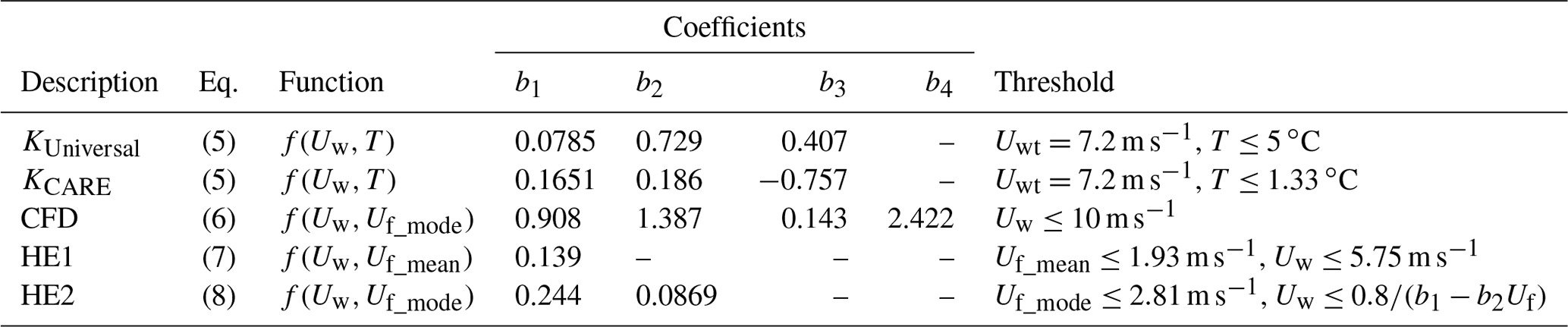
Using the same formulation, a site-specific transfer function based on wind speed and temperature was derived using the CARE dataset, for comparison with KUniversal. Best-fit regression coefficients were determined by varying the temperature threshold below 5 ∘C with the collection efficiency constrained to 1 above the threshold value. Solving Eq. (5a) for the temperature when the collection efficiency equals 1 provides an additional constraint on the b3 coefficient as a function of the b2 coefficient and temperature threshold (Tt).
The coefficients for the CARE site-specific transfer function, referred to as KCARE in this work, are provided in Table 1. The temperature threshold was varied over the measurement range in 0.01 ∘C increments to provide the lowest overall RMSE.
3.1 Precipitation type
Using the minutely POSS precipitation type output, events were classified as “rain”, “snow”, “mixed”, or “undefined” following the methodology in Sect. 2.4. The relative occurrence of different precipitation types as reported by the POSS for the event dataset is summarized in Table 2. The fall velocities in Table 2 were estimated by the POSS following the methodology in Sect. 2.4; the temperatures were estimated from a YSI44212 thermistor in an aspirated Stevenson screen as described in Sect. 2.2.
Table 2Mean fall velocities and temperatures of precipitation events by type classification.
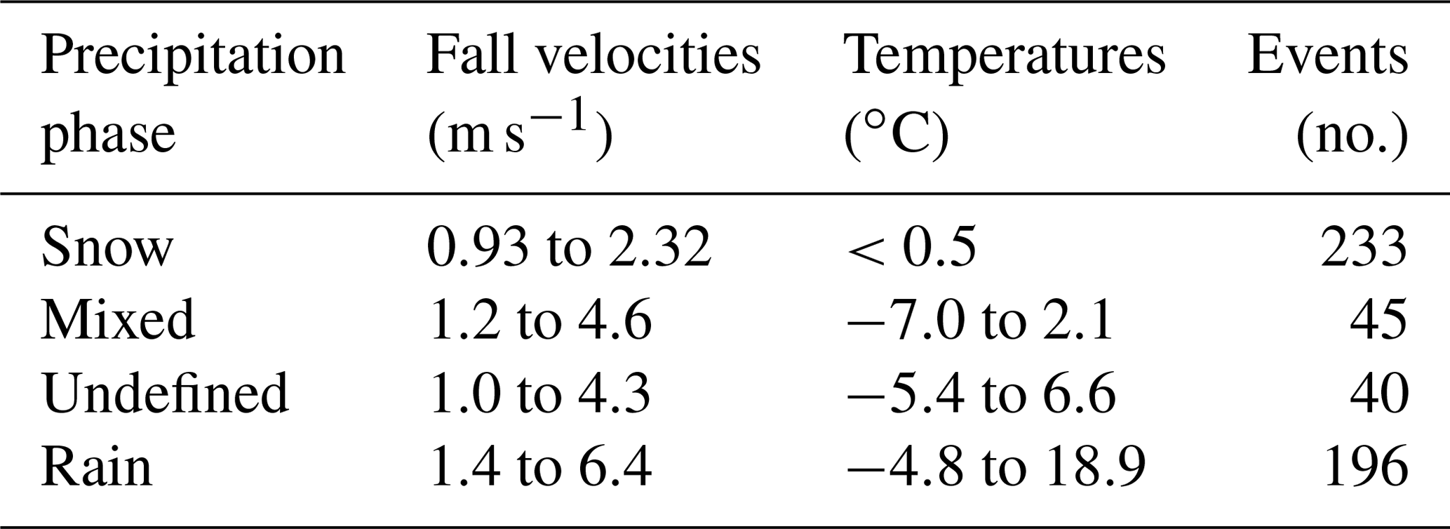
Based on the mean fall velocities and temperatures for each precipitation event (Fig. 1, Table 2), snow events occurred at temperatures below 0.5 ∘C and with fall velocities of 0.93 to 2.32 m s−1. Mixed events were characterized by mean temperatures between −7.0 and 2.1 ∘C and mean fall velocities between 1.2 and 4.6 m s−1, while undefined precipitation events occurred at mean temperatures between −5.4 and 6.6 ∘C and fall velocities between 1.0 and 4.3 m s−1. Rain events were characterized by mean temperatures between −4.8 and 18.9 ∘C and mean fall velocities between 1.4 and 6.4 m s−1. Over the temperature range between −5 and 2 ∘C, rain, snow, mixed, and undefined precipitation types were all present, demonstrating the challenge of estimating precipitation type using temperature alone (e.g. as done for the KUniversal and KCARE transfer functions). Within this temperature range, a wide variety of mean fall velocities, between 1 and 6 m s−1, is also apparent.
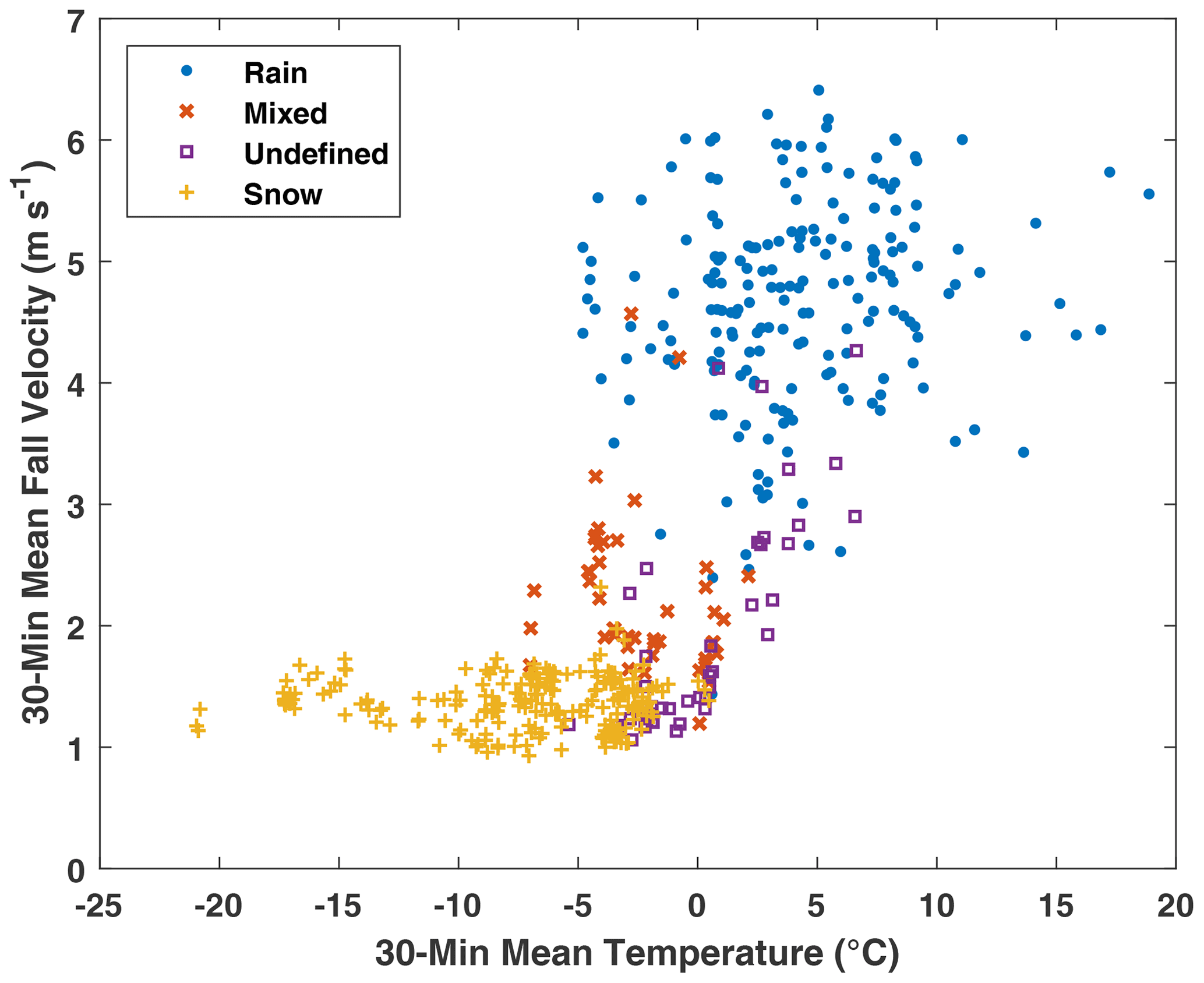
Figure 1Mean air temperature and fall velocity for 30 min events with rain, snow, mixed, and undefined precipitation (see Table 2 for summary).
3.2 Collection efficiency
3.2.1 CFD model
Simulations were run for wind speeds from 0 and 10 m s−1 and monodispersed hydrometeors with fall velocities between 0.25 and 10 m s−1. Details of the simulations are provided in Sect. S1.2. The numerical results for monodispersed hydrometeors demonstrate a clear dependence on the hydrometeor fall velocity (Fig. 2). Hydrometeors with higher fall velocities exhibit increased collection efficiency, and the collection efficiency tends to decrease with increasing wind speed. Rain, dry snow, and wet snow hydrometeors with 1.0 m s−1 fall velocity exhibit a similar collection efficiency decrease with increasing wind speed, despite differences in diameter, density, and mass. For rain and ice pellet hydrometeors with 5.0 m s−1 fall velocities, the results are close to 1 and nearly identical at all wind speeds, irrespective of differences in density. Here, the circles for rain overlap the squares for ice pellets in Fig. 2. Rain and wet snow with identical fall velocities between 1.0 and 2.5 m s−1 also exhibit similar results for wind speeds under 5 m s−1. Collection efficiency differences across all hydrometeor types with identical fall velocities are within 0.18, with root mean square differences of 0.05, over all wind speeds and hydrometeor fall velocities studied.

Figure 2Flow simulation results for Geonor unshielded gauge collection efficiency based on wind speed and hydrometeor fall velocity for rain, ice pellets, wet snow, dry snow, and CFD transfer function.
3.2.2 Experimental results
The unshielded gauge collection efficiency results are shown as a function of the 30 min DFAR event accumulations in Fig. 3a and stratified by precipitation type classification. The collection efficiency for rain shows less scatter and less uncertainty for higher reference precipitation accumulations. The dashed lines in Fig. 3a show the decrease in the collection efficiency uncertainty with increasing precipitation accumulation for a collection efficiency equal to 1 and a precipitation accumulation uncertainty of 0.1 mm (k=2) given by Eq. (3). These lines appear to capture the overall trend observed for rain events. The snowfall events show a markedly different trend, however, with collection efficiencies as low as 0.3.
The collection efficiency for all events as a function of mean wind speed and precipitation type classification is shown in Fig. 3b. For rain events, the collection efficiencies are close to 1. For snow, an approximately linear decrease in the collection efficiency with mean wind speed is apparent, with the collection efficiency decreasing to 0.3 at a wind speed of 5 m s−1. Mixed precipitation collection efficiencies span a range of values between those of rain and snow. For undefined precipitation, some events have collection efficiencies close to 1 at high wind speeds, similar to rain events, while others appear to decrease with increasing wind speed in a similar fashion to that observed for snow events.
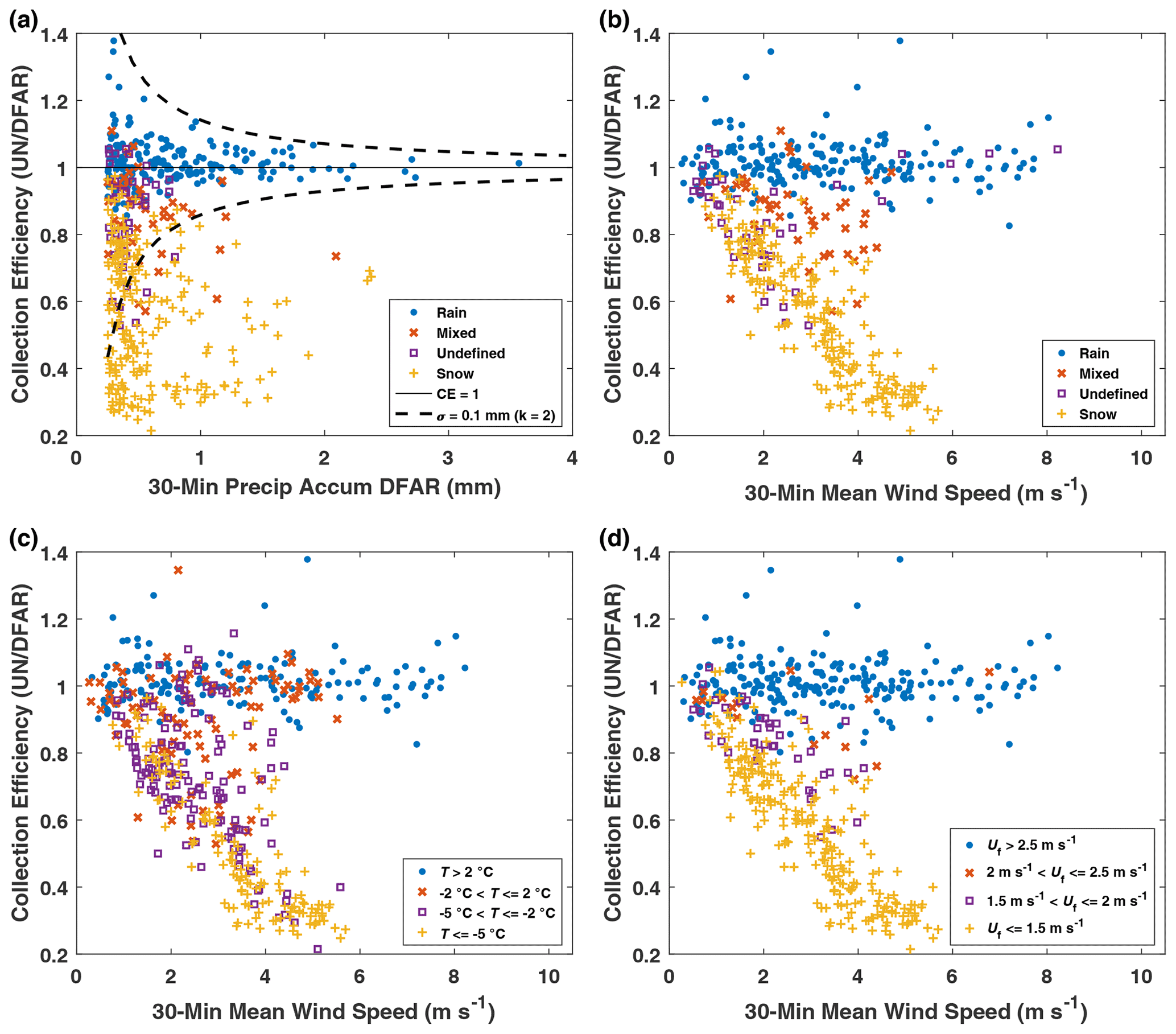
Figure 3Collection efficiency of the unshielded gauge as a function of (a) precipitation accumulation and event precipitation type (dashed lines illustrate accumulation uncertainty threshold), (b) wind speed and event precipitation type, (c) wind speed and mean air temperature T categories, and (d) wind speed and mode fall velocity Uf_mode categories.
The dependence of collection efficiencies on the mean wind speed over four separate mean temperature ranges is shown in Fig. 3c. For mean event temperatures above 2 ∘C, the collection efficiencies are generally close to 1, typical of rain. For temperatures between −5 and −2 ∘C and between −2 and 2 ∘C, a range of collection efficiency values are observed, from those typical of snow to those typical of rain. This variation is attributed to the wide range of fall velocities within this temperature range, which includes snow, rain, and mixed precipitation events (Fig. 3b). At colder temperatures, below −5 ∘C, collection efficiencies appear to decrease approximately linearly with wind speed, consistent with the trend observed for snow events in Fig. 3b.
Stratifying the collection efficiency results as a function of mean event wind speed by the mode fall velocity shows more distinct trends (Fig. 3d) relative to those observed when stratifying by temperature (Fig. 3c). Collection efficiencies are close to 1 for fall velocities greater than 2.5 m s−1, generally corresponding to rain. Conversely, fall velocities below 1.5 m s−1 show an approximately linear decrease in collection efficiency with increasing wind speed up to about 6 m s−1. A number of the values with higher collection efficiencies in this low fall velocity range correspond to mixed precipitation, where both snow and rain may be present. Between 1.5 and 2.5 m s−1 fall velocity, intermediate collection efficiency values are evident, with collection efficiencies transitioning from lower to higher values, despite a fewer number of observations in this range.
3.3 Derivation of fall velocity transfer functions from CE results
3.3.1 CFD model
The simulation results in Sect. 3.2.1 demonstrate that the collection efficiency is dependent on the free-stream wind speed (Uw) and hydrometeor fall velocity (Uf). The CFD transfer function, CECFD, is presented based on a polynomial fit to wind speed and an exponential hydrometeor fall velocity dependence, with both velocities having units of metres per second (m s−1).
This expression was selected due to its ability to capture the nonlinearity in the collection efficiency up to 10 m s−1 wind speed, as well as the nonlinear fall velocity dependence with collection efficiencies approaching 1 for higher fall velocities. Table 1 shows the best-fit coefficients (RMSE of 0.03) from a combined nonlinear regression for dry snow (0.5 and 0.75 m s−1 fall velocities), wet snow (1.0, 1.25, …, 2.5 m s−1 fall velocities), and rain (5 and 10 m s−1 fall velocities). A single CFD curve was used for each fall velocity in the fit to ensure that the transfer function was unbiased over the entire range of fall velocities studied.
The CFD transfer function is compared with the CFD results in Fig. 3. For hydrometeor fall velocities above 5.0 m s−1, the collection efficiency expression is within −0.13 and 0.10 of CFD results over all hydrometeor types. For fall velocities between 1.25 and 2.5 m s−1, the fit is within ±0.06 over all wind speeds. For fall velocities of 0.25 to 1.0 m s−1, the fit captures the rapid decrease in collection efficiency with wind speed well overall, with a maximum difference of 0.16 for dry snow at 5 m s−1 wind speed. The CFD transfer function captures the collection efficiency trends for the different hydrometeor types well, with RMSE values of 0.04 for rain, 0.02 for ice pellets, 0.02 for wet snow, and 0.05 for dry snow.
The CFD transfer function dependence with fall velocity is shown in Fig. 4. For a given wind speed, the collection efficiency increases nonlinearly with hydrometeor fall velocity. For fall velocities above 3 m s−1, the collection efficiency is close to 1. The collection efficiency rapidly decreases as the fall velocity is reduced, particularly below 2.5 m s−1 fall velocity. Increasing the wind speed decreases the collection efficiency.
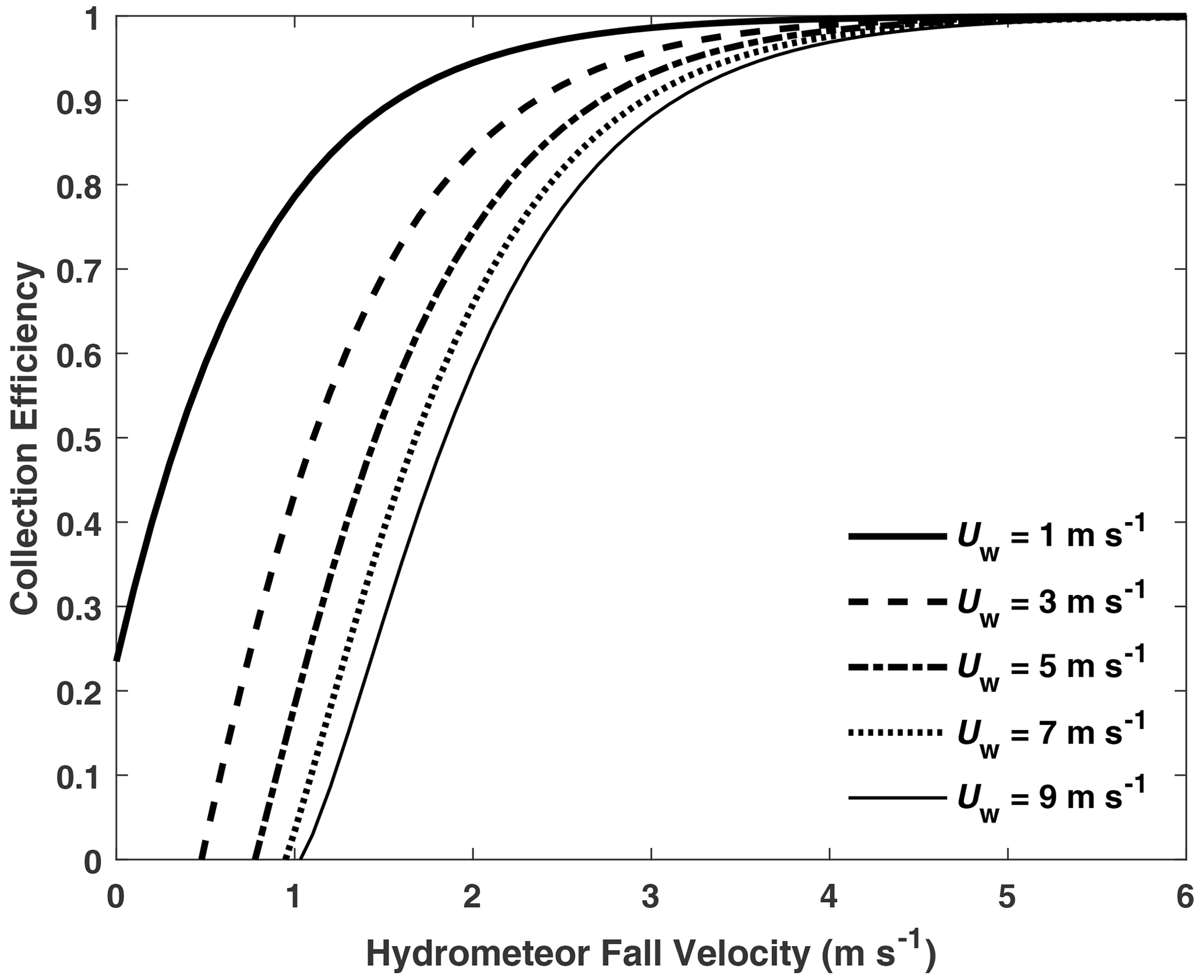
Figure 4Geonor unshielded gauge collection efficiency for the exponential fit model with hydrometeor fall velocity and wind speed.
To extend the approach from monodispersed to polydispersed hydrometeors, integral forms of the collection efficiency expression with wind speed and fall velocity dependence were defined for rain and snow, as detailed in Sect. S1.3. Using these expressions, collection efficiencies were derived for specified hydrometeor types and precipitation intensities over wind speeds from 0 to 10 m s−1. Figure 5 shows the integral collection efficiency as a function of hydrometeor fall velocity for precipitation type (thunderstorm rain, orographic rain, dendrites and aggregates of plates, rimed dendrites, and dendrites), precipitation intensity (0.1 to 20 mm h−1 for rainfall and 0.5 to 2.5 mm h−1 for snowfall), and wind speed (1, 3, and 6 m s−1). Here, the fall velocity at the median volume diameter is used as an estimate for the fall velocity distribution. The results take a similar form to that of the CFD transfer function shown in Fig. 4, with collection efficiencies increasing nonlinearly with hydrometeor fall velocity for a given wind speed. Dendrites, with the lowest fall velocity, exhibit the lowest integral collection efficiency. Rimed dendrites and dendrites and aggregates of plates with higher fall velocity exhibit higher collection efficiency. In this fall velocity range below 1.5 m s−1, the collection efficiency rapidly increases approximately linearly with fall velocity. For orographic rain and thunderstorm rain, with even higher fall velocity, the integral collection efficiency nonlinearly approaches 1. As wind speeds increase from 1 to 6 m s−1, collection efficiencies for all precipitation types are shifted down at the lower end of the fall velocity spectrum below 2 m s−1 and still converge to 1 at higher fall velocities, close to 5 m s−1.

Figure 5Integral Geonor unshielded gauge collection efficiency with hydrometeor fall velocity at median volume diameter for rainfall and snowfall types at 1, 3, and 6 m s−1 wind speeds.
For snowfall, the integral collection efficiency difference across dendrites, rimed dendrites, and dendrites and aggregates of plates is less than 0.06 for 0.5, 1.5, and 2.5 mm h−1 precipitation intensities at 6 m s−1 wind speed and within 0.03 for the same precipitation intensities at 3 m s−1 wind speed. For rainfall, the integral collection efficiency difference is less than 0.01 at 3.8 m s−1 fall velocity, where orographic rain and thunderstorm rain overlap. Orographic rain exhibits median volume diameter fall velocities between 1.6 and 3.9 m s−1 for precipitation intensities from 0.1 to 10 mm h−1. Thunderstorm rain exhibits median volume diameter fall velocities between 3.8 and 5.6 m s−1 for precipitation intensities from 1 to 20 mm h−1.
3.3.2 Experimental results
Two additional transfer functions were formulated based on the apparent linear dependence of CE on wind speed for different hydrometeor fall velocity regimes observed in experimental results (Fig. 3d). These functions are applicable to all hydrometeor types and have different fall velocity thresholds to describe the transition of precipitation phase from the lower fall velocities characteristic of snow to the higher fall velocities characteristic of rain and mixed precipitation.
The first transfer function, referred to as HE1, is based on the assumption of a linear decrease in collection efficiency (CEHE1) with wind speed (Uw) for hydrometeors with mean fall velocity (Uf_mean) below 1.93 m s−1, generally corresponding to snowfall. This linear decrease is extrapolated up to a 5.75 m s−1 wind speed threshold (Eq. 7a), above which the collection efficiency for snowfall is 0.2 (Eq. 7b), following the general approach of Kochendorfer et al. (2017a). For hydrometeors with mean fall velocity greater than 1.93 m s−1, corresponding to mixed and liquid precipitation, the collection efficiency is 1 (Eq. 7c). The fall velocity threshold was varied over the measurement fall velocity range in 0.01 m s−1 increments, with the threshold of 1.93 m s−1 found to provide the lowest overall RMSE.
The second transfer function, referred to as HE2, adds another dimension to describe the slope of the linear decrease in CE with increasing wind speed: the hydrometeor fall velocity. For mode fall velocity (Uf_mode) below 2.81 m s−1 and wind speed Uw below the threshold value, which is also dependent on the fall velocity, the collection efficiency (CEHE2) is assumed to decrease linearly with decreasing wind speed for a given hydrometeor fall velocity (Eq. 8a). For mode fall velocity below 2.81 m s−1 and wind speed above the threshold value, the collection efficiency is 0.2 (Eq. 8b). For mode fall velocity above 2.81 m s−1, the collection efficiency is equal to 1 (Eq. 8c). The fall velocity threshold was varied over the measurement fall velocity range in 0.01 m s−1 increments, with the threshold of 2.81 m s−1 found to provide the lowest overall RMSE.
3.4 Assessment of transfer functions
3.4.1 Collection efficiency
Observed collection efficiencies were compared with adjusted values using both existing transfer functions from SPICE and those presented in this work. Results are presented in Fig. 6, with relevant transfer function parameters compiled in Table 1 and resulting bias errors, root mean square errors, and correlation coefficients (r) presented in Table 3. To further contextualize the assessment of the different transfer functions, the RMSE results are presented for different precipitation classifications, temperature ranges, and fall velocity ranges in Table 4.
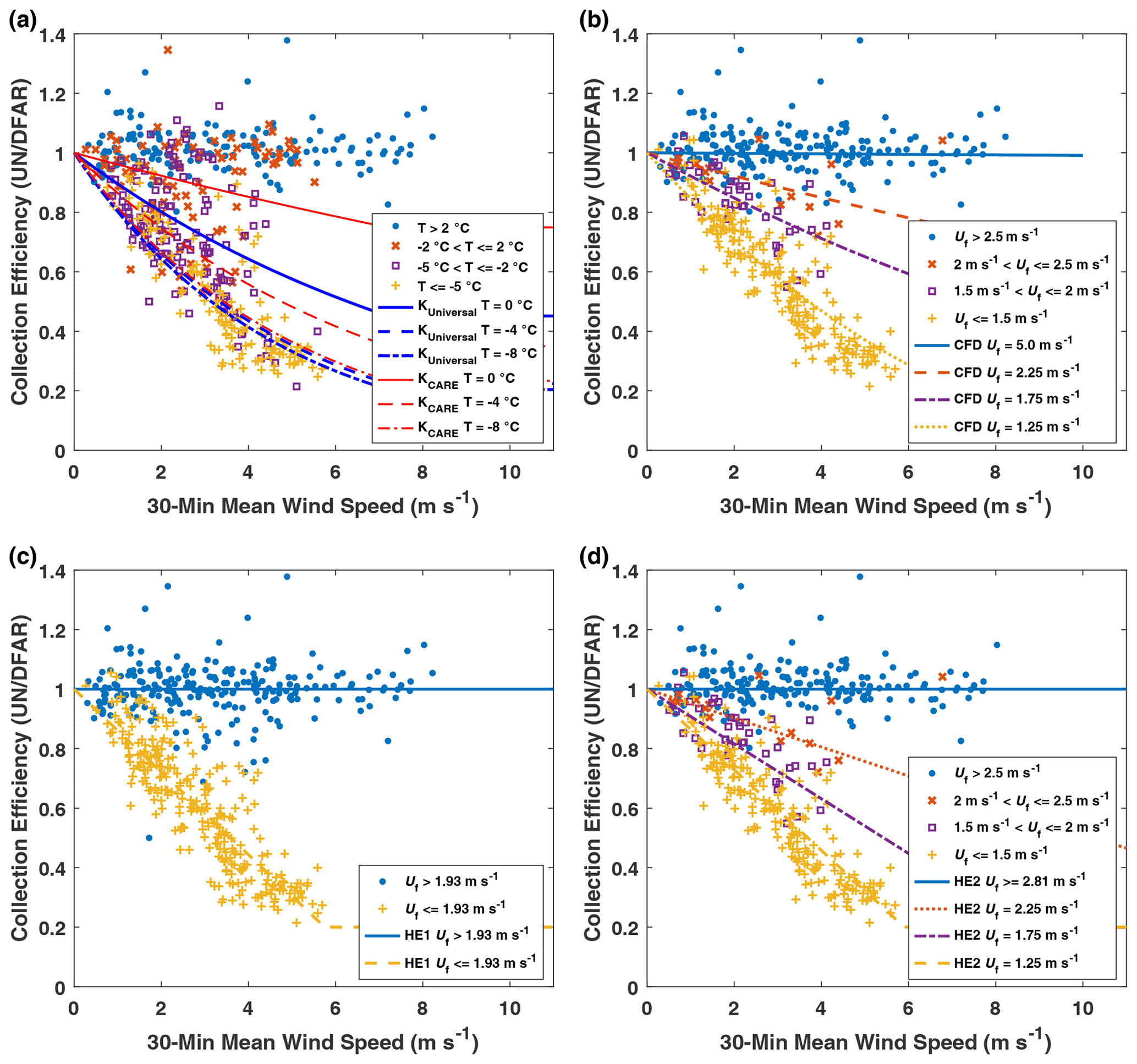
Figure 6Collection efficiency of unshielded gauge as a function of wind speed for (a) mean air temperature T categories for the KUniversal and KCARE transfer functions, (b) mode fall velocity Uf_mode categories with the CFD transfer function, (c) mean fall velocity Uf_mean categories for the HE1 transfer function, and (d) mode fall velocity Uf_mode categories with the HE2 transfer function.
Table 3Unshielded gauge 30 min event bias error (BE), root mean square error (RMSE), correlation coefficient (r), and number of events (N) for collection efficiency and precipitation accumulation between the unshielded and reference DFAR shielded Geonor T-200B3 gauge for unadjusted comparison, KUniversal transfer function with wind speed and air temperature dependence, KCARE transfer function with wind speed and air temperature dependence, present study CFD transfer function with wind speed and mode fall velocity dependence, HE1 transfer function with wind speed and mean fall velocity dependence, and HE2 transfer function with wind speed and mode fall velocity dependence. Statistics are based on the comparison of experimental results from the CARE site between 1 November and 30 April 2013/14 and 2014/15.
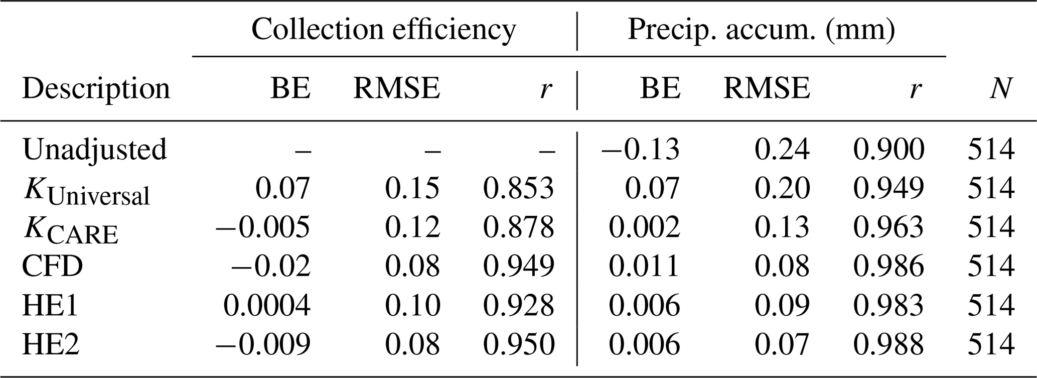
Table 4Unshielded gauge 30 min event collection efficiency RMSE results stratified by (a) POSS precipitation type, (b) temperature, and (c) fall velocity. Results are shown for KUniversal transfer function with wind speed and air temperature dependence, KCARE transfer function with wind speed and air temperature dependence, present study CFD transfer function with wind speed and mode fall velocity dependence, HE1 transfer function with wind speed and mean fall velocity dependence, and HE2 transfer function with wind speed and mode fall velocity dependence. Statistics are based on the comparison of experimental results from the CARE site between 1 November and 30 April 2013/14 and 2014/15.
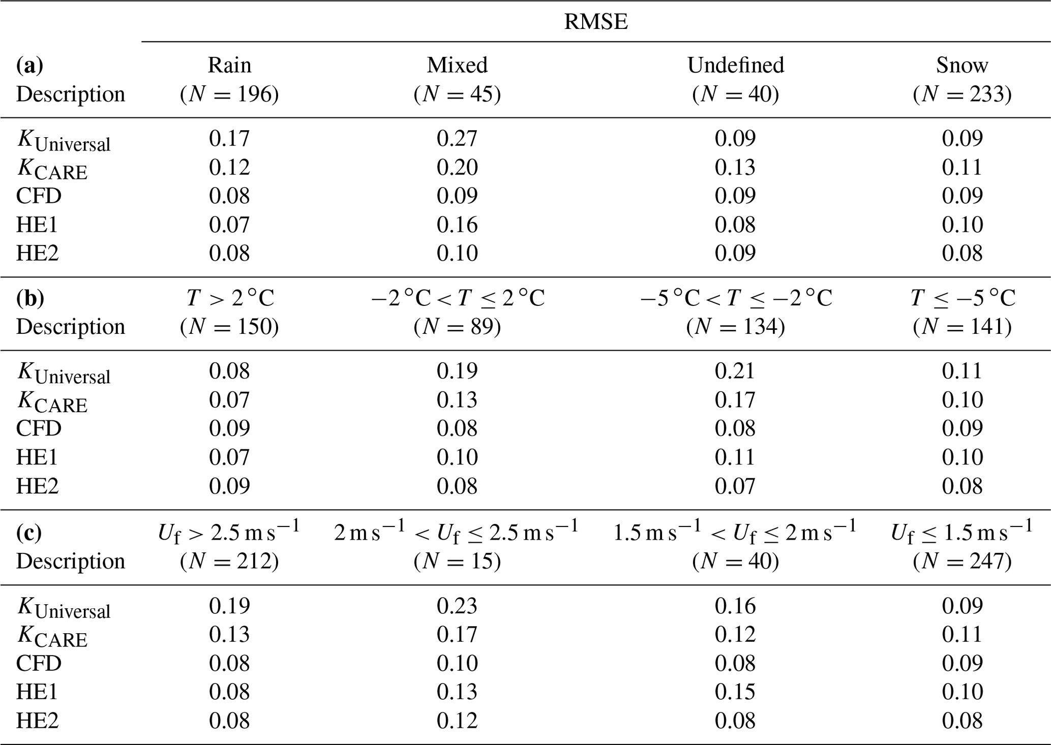
Both KUniversal and the climate-specific KCARE transfer function have continuous temperature dependence and display similar profiles at −8 ∘C, with the collection efficiency for the KCARE transfer function decreasing more gradually with wind speed compared to the KUniversal transfer function at −4 and 0 ∘C (Fig. 6a). Using the approach outlined in Sect. 2.5, a temperature threshold (Tt) of 1.33 ∘C for the best-fit KCARE transfer function was found to minimize the precipitation accumulation RMSE. The overall collection efficiency root mean square error is reduced from 0.15 for the KUniversal transfer function to 0.12 for the KCARE transfer function (Table 3). The bias error is also reduced from 0.07 for the KUniversal transfer function to −0.005 for the best-fit KCARE transfer function. For KUniversal and KCARE, respectively, the RMSE is reduced from 0.17 to 0.12 for rain and from 0.27 to 0.20 for mixed precipitation, with slightly elevated RMSE from 0.09 to 0.13 for undefined precipitation and 0.09 to 0.11 for snow (Table 4a). For mean event temperatures between −2 and 2 ∘C, and between −5 and −2 ∘C, respectively, the RMSE values of 0.19 and 0.21 for the KUniversal transfer function are relatively large compared to the 0.13 and 0.17 values for the KCARE transfer function (Table 4b). This results from the more gradual decrease in the KCARE transfer function with wind speed over these temperature ranges (Fig. 6a).
A comparison of the CFD transfer function with observed CE is shown in Fig. 6b. Overall, the measured data have less scatter when stratified by fall velocity than when stratified by temperature (Table 3, Fig. 6a and b). The CFD transfer function provides a lower overall RMSE (0.08) and higher r (0.949) relative to the KUniversal and KCARE transfer functions based on temperature. Reductions in the collection efficiency RMSE using the CFD transfer function are most pronounced for rain and mixed precipitation (Table 4a) and for mean event temperatures between −2 and 2 ∘C and between −5 and −2 ∘C (Table 4b) compared with the KUniversal and KCARE functions. Collection efficiency RMSE values are between 0.08 and 0.10 over all fall velocity classes, despite fewer numbers of events with fall velocities between 1.5 and 2.5 m s−1 (Table 4c).
The HE1 transfer function provides good agreement with observed data in the mean fall velocity regimes relevant to snow and rain (Fig. 6c), resulting in an overall RMSE of 0.10, BE of 0.0004, and r of 0.928 (Table 3). The RMSE for mixed precipitation is 0.16, which is lower than that of the KCARE transfer function with temperature (0.20) but higher that of the CFD model (0.09), which varies continuously with fall velocity (Table 4a).
The HE2 function better captures the observed collection efficiencies for mode fall velocities between the snow and rain regimes (Fig. 6d), improving the overall RMSE to 0.08 and r to 0.95, while increasing slightly the BE (−0.009) relative to HE1 (Table 3). Note the distinction between mean fall velocity for HE1 and mode fall velocity for HE2 (and CFD). In general, the Doppler frequency spectrum tends to be skewed such that mode fall velocities are slightly lower than the mean fall velocities, impacting the fits to observed data. The HE2 transfer function provides similar results to that of the CFD transfer function, with slightly higher RMSE values for mixed precipitation and slightly reduced RMSE values for snow (Table 4a) and temperatures below −2 ∘C (Table 4b). For intermediate fall velocities between 2.0 and 2.5 m s−1, the HE2 transfer function, with a linear change in collection efficiency with fall velocity, has a higher RMSE (0.12) than that for the CFD function (0.10), which exhibits a nonlinear change in collection efficiency with fall velocity (Table 4c). Only 15 events were recorded in this intermediate fall velocity range with higher uncertainty relative to the CFD function. In contrast, 212 events were recorded at fall velocities above 2.5 m s−1 and 247 events at fall velocities below 1.5 m s−1, representing a greater proportion of the events with lower RMSE relative to the CFD function.
3.4.2 Precipitation accumulation
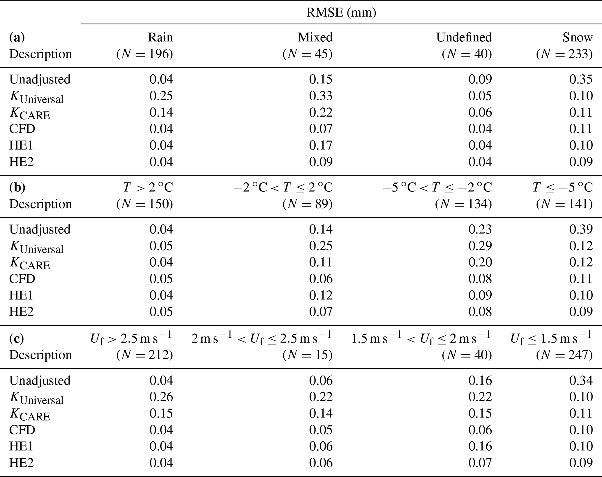
The unadjusted and adjusted accumulated precipitation values are compared with reference DFAR accumulation measurements in Fig. 7. Bias, RMSE, and correlation coefficient results are shown in Table 3. Similar to the approach for assessing transfer functions based on collection efficiency results in Sect. 3.4.1, the precipitation accumulation RMSE results for each transfer function are assessed by precipitation classification, temperature range, and fall velocity range in Table 5.
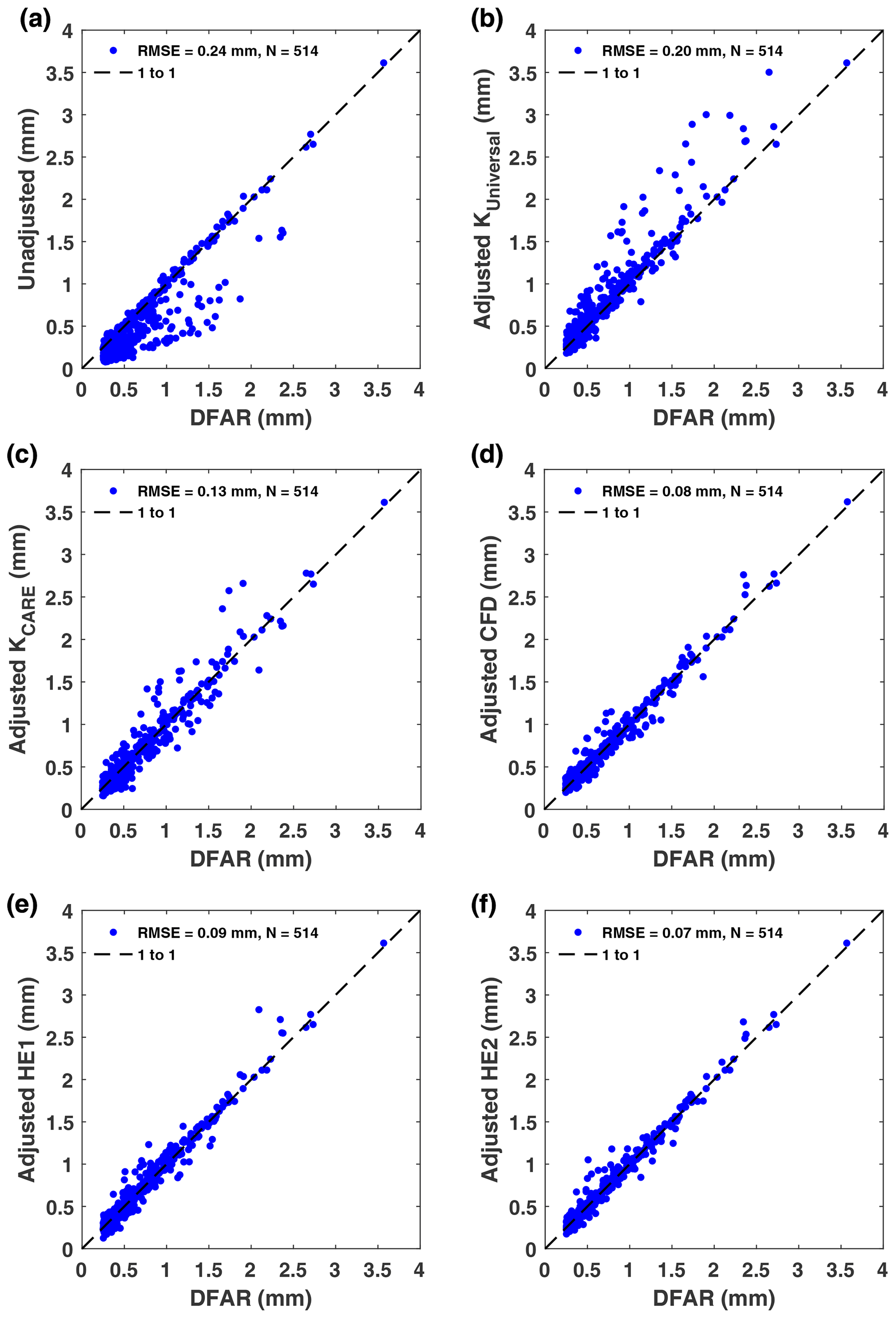
Figure 7Unshielded and reference DFAR 30 min event precipitation accumulation comparison for (a) unadjusted precipitation accumulation, (b) KUniversal continuous transfer function with wind speed and air temperature dependence, (c) KCARE continuous transfer function with wind speed and air temperature dependence, (d) CFD transfer function with wind speed and fall velocity dependence, (e) HE1 transfer function with wind speed and fall velocity dependence, and (f) HE2 transfer function with wind speed and fall velocity dependence.
Table 5Unshielded gauge 30 min event RMSE (mm) results stratified by (a) POSS precipitation type, (b) temperature, and (c) fall velocity. Results are shown for unadjusted comparison, KUniversal transfer function with wind speed and air temperature dependence, KCARE transfer function with wind speed and air temperature dependence, present study CFD transfer function with wind speed and mode fall velocity dependence, HE1 transfer function with wind speed and mean fall velocity dependence, and HE2 transfer function with wind speed and mode fall velocity dependence. Statistics are based on the comparison of experimental results from the CARE site between 1 November and 30 April 2013/14 and 2014/15.
In the comparison of unadjusted accumulation measurements with reference values (Fig. 7a), some values fall along the 1-to-1 line, while others are considerably lower. The values along the 1-to-1 line generally correspond to rain events with high precipitation fall velocity or to events with low mean wind speeds. The RMSE for the unadjusted unshielded gauge measurements relative to the DFAR is 0.24 mm, with a bias error of −0.13 mm and correlation coefficient of 0.900 (Table 3).
Using the KUniversal transfer function, with wind and temperature dependence, shifts the adjusted values up to and above the 1-to-1 line (Fig. 7b). This yields a positive bias error of 0.07 mm, reduced RMSE of 0.20 mm, and correlation coefficient of 0.949 (Table 3) relative to the unadjusted measurements (Fig. 7a). While the KUniversal transfer function greatly reduces the RMSE for snow from 0.35 to 0.10 mm compared with unadjusted values, the RMSE is increased from 0.04 to 0.25 mm for rain and from 0.15 to 0.33 mm for mixed precipitation (Table 5a). Compared with the unadjusted results, RMSE increases for the KUniversal function are also apparent for temperatures between −2 and 2 ∘C and between −5 and −2 ∘C (Table 5b) and for fall velocities greater than 1.5 m s−1 (Table 5c).
Applying the site-specific KCARE transfer function, based on the best-fit results to the CARE SPICE dataset, results in a reduced bias error of 0.002 mm, lower RMSE of 0.13 mm, and higher correlation coefficient of 0.963 (Table 3) relative to the KUniversal results, with the scatter in adjusted accumulations more evenly balanced across the 1-to-1 line (Fig. 7c). The scatter in adjusted values using the KCARE transfer function results primarily from mixed precipitation (Table 5a) at temperatures between −5 and −2 ∘C (Table 5b). Compared to the KUniversal transfer function, the KCARE transfer function has lower RMSE values for rain (0.14 mm) and mixed precipitation (0.22 mm), with 0.01 mm higher RMSE for undefined precipitation and snow (Table 5a). The more rapid increase in collection efficiency with temperature for KCARE relative to KUniversal reduces the overadjustment of some of the rain and mixed precipitation events at temperatures between −5 and −2 ∘C, at the expense of the underadjustment of some snow events in this temperature range. It is also worth noting that the adjusted precipitation accumulation RMSE for the KCARE transfer function is larger than that for unadjusted results for rain and mixed precipitation, similar to the results for KUniversal. Both the KUniversal and KCARE transfer functions with temperature show signs of heteroscedasticity, with an increased spread of values with increasing magnitude of event precipitation accumulation.
Applying the CFD transfer function results in a greatly reduced spread of values about the 1-to-1 line (Fig. 7d). The spread does not appear to increase with increasing precipitation accumulation. The overall RMSE is reduced to 0.08 mm, 2.5 times lower than that for the KUniversal transfer function, with a bias error of 0.011 mm and correlation coefficient of 0.986 (Table 3). The RMSE is reduced from 0.25 mm for the KUniversal transfer function to 0.04 mm using the CFD transfer function for rain and from 0.33 to 0.07 mm (4.7 times lower) for mixed precipitation, while RMSE results for undefined precipitation and snow are within 0.01 mm (Table 5a). Reductions in the RMSE using the CFD transfer function compared with the KUniversal transfer function are most pronounced for mean event temperatures between −5 and 2 ∘C (Table 5b). Over this temperature range, rain, mixed precipitation, and snow may be present, corresponding to a wide range of fall velocities and collection efficiencies. The CFD transfer function is better able to distinguish among these precipitation types – and their respective collection efficiencies – based on its dependence on hydrometeor fall velocity. Across the fall velocity classifications in Table 5c, the RMSE using the CFD transfer function increases from 0.04 mm for fall velocities greater than 2.5 m s−1 to 0.10 mm for fall velocities less than 1.5 m s−1. As shown in Table 5c, the RMSE for the CFD transfer function matches the value for unadjusted measurements at fall velocities greater than 2.5 m s−1, where collection efficiencies are close to 1. At lower fall velocities, where the bias due to gauge undercatch is more prevalent, the RMSE values for the CFD function are lower than those for the unadjusted measurements.
Using the HE1 transfer function results in similar overall improvement in the agreement between adjusted and DFAR accumulation values as observed for the CFD function (Fig. 7e). The adjusted values appear to be distributed symmetrically about the 1-to-1 line. Furthermore, there is close agreement over the full range of accumulation values; that is, the spread in values does not increase with the magnitude of precipitation accumulation. This results in a lower RMSE of 0.09 mm and a higher correlation coefficient of 0.983 relative to the KCARE transfer function results. While the RMSE for rain (0.04 mm) using the HE1 transfer function is improved compared with the KCARE transfer function results, the RMSE for mixed precipitation is only marginally better (0.17 mm).
Applying the HE2 transfer function provides further improvement, with adjusted accumulation values more tightly clustered around the 1-to-1 line (Fig. 7f). The overall RMSE is 0.07 mm, which is 3.3 times lower than that for the unadjusted unshielded gauge measurements and 1.8 times lower than the KCARE transfer function based on mean event temperature and wind speed. The HE2 transfer function exhibits the lowest overall RMSE for snow (0.09 mm), with a RMSE of 0.09 mm for mixed precipitation, which is slightly higher than that for the CFD function (0.07 mm) but much lower than that for the KCARE (0.22 mm) and HE1 (0.17 mm) transfer functions. Further, the correlation coefficient of 0.988 is the highest among the transfer functions assessed.
The resulting CARE dataset from this study (Hoover at al., 2021) includes the reference, adjusted, and unadjusted (unshielded) precipitation accumulation with event start time, scalar average gauge height wind speed, mean air temperature, POSS precipitation type, POSS mode fall velocity, and POSS mean fall velocity for each 30 min precipitation event.
4.1 CFD model
The numerical model results for monodispersed hydrometeors capture the three-dimensional airflow and hydrometeor kinematics and illustrate the reductions in collection efficiency with increasing wind speed and decreasing hydrometeor fall velocity (Fig. 2). These results demonstrate that collection efficiencies are similar for different hydrometeor types with different sizes, densities, masses, and drag values (spherical drag model) but similar fall velocities. This enables the characterization of collection efficiency independent of hydrometeor characteristics other than fall velocity, allowing for the broad application of transfer functions with wind speed and fall velocity dependence to various hydrometeor types.
A slight nonlinearity in the collection efficiency relationship with wind speed is apparent in Fig. 2, with the collection efficiency decreasing more rapidly at lower wind speeds and more gradually at higher wind speeds. This wind speed dependence has been demonstrated in previous studies (Nešpor and Sevruk, 1999; Thériault et al., 2012; Colli et al., 2016a; Baghapour et al., 2017) and is generally attributed to the three-dimensional velocity profile around the gauge influencing the trajectories and catchment of incoming hydrometeors. A strong nonlinear dependence on the hydrometeor fall velocity is apparent in Figs. 3 and 5. Hydrometeors with fall velocities above 5 m s−1 exhibit collection efficiencies close to 1, while lower hydrometeor fall velocities influence the rate of decrease of collection efficiency with wind speed. Collection efficiency decreases are most pronounced below 2.0 m s−1 hydrometeor fall velocity, where a wide range of collection efficiencies are possible. This demonstrates the challenge in adjusting liquid, solid, and mixed precipitation accumulations in situations where different hydrometeor types and sizes – and with very different fall velocities – can occur. These findings support the conclusions of Thériault et al. (2012), who demonstrated large collection efficiency differences across dry snow and wet snow hydrometeors with different terminal velocities. The present findings also support those of Nešpor and Sevruk (1999), who showed that the wind-induced error increases rapidly for smaller raindrop sizes with lower terminal velocities.
The CFD transfer function presented in Eq. (6) (coefficients in Table 1) is based on the computational fluid dynamics results for an unshielded Geonor T-200B3 600 mm capacity precipitation gauge for wind speeds up to 10 m s−1. The CFD transfer function captures the nonlinear change in collection efficiency well, with wind speed and hydrometeor fall velocity observed in the numerical model results across rain, ice pellet, wet snow, and dry snow hydrometeor types (Fig. 2). This expression was derived from simulation results up to 10 m s−1 wind speed and should be used with caution at higher wind speeds. Further, this transfer function has not been assessed experimentally for snow above 6 m s−1 wind speed in the present study for the CARE dataset. Adjusted precipitation accumulation estimates in this regime, where fall velocities are low and wind speeds are high, can be highly uncertain and should be treated with caution (Smith et al., 2020). Assessment of the transfer function at other sites under such conditions is an area for future work. Application to other gauge or shield combinations should also be investigated, as the flow dynamics around the gauge orifice are dependent on the specific gauge and shield geometry.
The CFD transfer function formulation based on the fall velocity can be applied broadly across rain and snow types for the unshielded Geonor gauge configuration. These results are based on time-averaged simulations, which provide an estimate of the mean velocities through the domain and have been shown to provide good overall agreement with experimental results (Baghapour et al., 2017). Further study using LES models, which can better resolve the eddy dynamics and temporal variations in the flow, and under different boundary conditions and turbulence scales representing different site conditions is recommended to better understand the collection efficiency under conditions with high wind speeds and low hydrometeor fall velocities.
Integral collection efficiency differences across precipitation types are small when stratified by wind speed and hydrometeor fall velocity (Fig. 5). This results from the ability of the hydrometeor fall velocity to capture differences in the integral collection efficiency across different hydrometeor types and precipitation intensities. The small differences in collection efficiency across different hydrometeor types with the same fall velocity are attributed to the varying contribution from higher fall velocity hydrometeors, with collection efficiencies approaching 1, in the mass-weighted distribution of hydrometeor fall velocities. The results in Fig. 5 follow the general nonlinear profile of the CFD transfer function (Eq. 6, Fig. 4), with the hydrometeor fall velocity defining the integral collection efficiency magnitude for a given wind speed. Results for the same wind speed range and precipitation types that are stratified by wind speed and precipitation intensity, and by wind speed alone, are provided in Sect. S2.2 and discussed in Sect. S3.2; these results show much larger variability across hydrometeor types relative to those in Fig. 5.
4.2 Assessment of transfer functions
Transfer functions were derived using accumulated precipitation amounts reported by automatic weighing precipitation gauges over 30 min periods. This approach is consistent with that used in SPICE (Nitu et al., 2018) and the related derivation of transfer functions (Kochendorfer et al., 2017a). While automatic precipitation gauges can report at a temporal resolution of 1 min, or even higher, the extension of the transfer function derivation and evaluation to other temporal periods, or different accumulation thresholds, is beyond the scope of this work.
The Kochendorfer et al. (2017a) universal transfer function with wind speed and air temperature dependence, KUniversal, was derived from measurements at eight SPICE sites in the interest of making the transfer function broadly applicable across different climates. This broad applicability is furthered by the widespread availability of air temperature and wind speed measurements at meteorological stations. Recent studies have demonstrated that the performance of KUniversal can vary substantially by site (Smith et al., 2020). Therefore, climate-specific KCARE transfer function coefficients were also derived for comparison in the present study.
The KCARE transfer function has a lower temperature threshold and exhibits larger increases in collection efficiency with increasing temperature relative to KUniversal (Fig. 6a). These differences improved the overall RMSE for KCARE by reducing the overadjustment of some rain and mixed precipitation events; however, this improvement came at the expense of underadjusting some snow events at warmer temperatures. The use of this approach warrants further study over longer periods to better understand the performance impacts of seasonal variability and assessment at other sites and climate regions with different precipitation characteristics and proportions.
Both the KUniversal and KCARE transfer functions performed well for snow but were limited by their ability to distinguish among snow, rain, and mixed precipitation at temperatures between −5 and 2 ∘C. The largest uncertainties in collection efficiency and adjusted accumulation estimates were observed over this temperature range. Adjustments using wind speed and hydrometeor fall velocity, however, addressed this shortcoming and provided improved collection efficiency and adjusted accumulation estimates. The CFD transfer function, derived from time-averaged numerical simulation results over a wide range of wind speeds and hydrometeor fall velocities, resulted in low RMSE values overall and across rain, snow, mixed, and undefined precipitation types. These results reinforce the fundamental importance of both wind speed and hydrometeor fall velocity on gauge collection efficiency demonstrated by the CFD model results and results from earlier studies (Nešpor and Sevruk, 1999; Thériault et al., 2012).
The CFD transfer function exhibited the lowest RMSE of all transfer functions for mixed precipitation and for intermediate fall velocities between 1.5 and 2.5 m s−1 (Table 4c), which is attributed to its nonlinear increase in collection efficiency with fall velocity. As this transfer function was derived theoretically, it is applicable across different sites and climate regimes with different types and relative proportions of hydrometeors. The present results also support the methodology for the CFD model, which can be extended to other shield and gauge combinations. For larger shields, it may be important to employ a more realistic vertical wind profile, with a zero-slip boundary condition at the earth's surface.
The HE1 transfer function showed good results for snow, supporting its use for the unshielded gauge. This approach is straightforward to implement based on its simplicity and is less reliant on the accuracy of fall velocity estimates beyond the fall velocity threshold. The collection efficiency for the HE1 transfer function decreases to 0.2 at a wind speed of 5.75 m s−1. This demonstrates the challenge of adjusting unshielded gauge snow measurements at windy sites, where the captured accumulations may be small relative to gauge uncertainties. This can lead to large uncertainty in adjusted measurements, as demonstrated by other studies applying transfer functions to unshielded gauge measurements at windy sites (Smith et al., 2020). The CFD transfer function results suggest a gradual decrease in collection efficiency at higher wind speeds compared with the HE1 transfer function, as some hydrometeors with higher fall velocities are still able to be captured by the gauge; however, these accumulations remain small relative to gauge uncertainties, particularly in windy conditions, making them difficult to assess experimentally. Further testing at other sites is recommended to better understand the collection efficiency for low fall velocity hydrometeors (light snow) under windy conditions above 6 m s−1, which were not available in the CARE dataset.
A limitation of the HE1 transfer function is the minimal improvement in the RMSE for mixed precipitation and fall velocities between 1.5 and 2.0 m s−1 relative to the KCARE function. This is due to the overadjustment of mixed precipitation events with fall velocities slightly below the cutoff value and the underadjustment of mixed precipitation events with fall velocities slightly above the cutoff. While the RMSE for mixed precipitation is still lower than that for adjustments based on temperature and wind speed (KUniversal, KCARE), further improvements are obtained using transfer functions with continuous fall velocity dependence – specifically, the CFD and HE2 transfer functions.
The HE2 transfer function, with a linear increase in collection efficiency with fall velocity, yields a greater reduction in the RMSE for mixed precipitation relative to the HE1 transfer function. The HE2 transfer function results show a higher RMSE for mixed precipitation than those for the CFD function, possibly due to the nonlinearity in the latter with fall velocity. The HE2 transfer function, however, yields the best RMSE results for snow, temperatures below −5 ∘C, and fall velocities below 1.5 m s−1. Adjusted uncertainties for snow are approximately 2 times higher than those for rain and show similar trends with increasing temperature and decreasing fall velocity. The former may be due to the lower event accumulations and greater adjustments for snow relative to rain, with measured values in closer proximity to the gauge uncertainty. The present approach of estimating the fall velocity using the POSS appears to perform well, overall; however, further study to better characterize the fall velocity distribution and changes over 30 min time periods could lead to further improvements in the model under specific conditions such as mixed precipitation. While this transfer function was derived using the CARE dataset, it is more universally applicable than adjustments based on temperature, for which the relative proportions of rain, snow, and mixed precipitation at warmer temperatures can influence fit results. Further testing at other sites is recommended to assess this in different climate regions, with different hydrometeor types and associated fall velocities.
4.3 Application to operational networks
It is evident that the performance of catchment-type precipitation gauges is dependent on wind speed and the aerodynamic properties of both the gauge and incident hydrometeors (Nešpor and Sevruk, 1999; Thériault et al., 2012; Colli et al., 2016b). The modelling results of this study demonstrated this dependence from a theoretical perspective, resulting in a transfer function that incorporates hydrometeor fall velocity. The experimental results validated this approach, which resulted in improved precipitation estimates from an unshielded gauge relative to those using surface temperature as a proxy for precipitation phase or type. Indeed, the use of surface temperature in this manner can be instructive (Kienzle, 2008; Harder and Pomeroy, 2013) but does not capture the conditions defining hydrometeor initiation and growth aloft (Stewart et al., 2015).
In this study, the fall velocity of hydrometeors reported by the POSS provided direct measurement of a key parameter related to the aerodynamics of the catchment process. In Canada, the POSS was deployed operationally to report present weather as part of an automatic weather station. In operational monitoring networks, the hydrometeor fall velocity can be provided by disdrometers (Loffler-Mang and Joss, 2000; Sheppard and Joe, 2000; Bloemink and Lanzinger, 2005; Nitu et al., 2018), vertically pointing Doppler radars (Biral, 2019), or multi-frequency radar techniques (Kneifel et al., 2015). Globally, other types of disdrometers (e.g. OTT Parsivel2, Thies Laser Precipitation Monitor) have been deployed operationally and can also provide hydrometeor fall velocities. The uncertainty in fall velocity estimates for different technologies, hydrometeor types, sizes, fall velocities, wind speeds, and wind directions remains to be assessed. These sensors can also be useful for reporting present weather and verifying the occurrence of precipitation based on their high sensitivity (Nitu et al., 2018; Sheppard and Joe, 2000).
The results from this study demonstrate that the combined use of accumulation reports from an unshielded weighing gauge with fall velocities reported by a disdrometer, wind speed measurements, and an appropriate transfer function can greatly reduce the uncertainty of precipitation accumulation measurements. The extension of the approach in the present study to shielded precipitation gauges or gauge designs with higher sensitivity may provide a means of further reducing the measurement uncertainty for automatic gauges in windy environments. Application to light snow events and different event durations are other areas for future study.
Hydrometeors exhibit a wide variety of habits, sizes, shapes, and densities, influencing their aerodynamics and, in turn, their ability to be captured by the gauge. Numerical modelling analysis for an unshielded Geonor T-200B3 600 mm precipitation gauge demonstrated that collection efficiencies are similar for different hydrometeor types with different sizes, densities, masses, and drag values but similar fall velocities. The model results illustrated that wind speed influences the updraft magnitude and local airflow around the gauge orifice, while fall velocity affects the approach angle and degree of coupling between the hydrometeor trajectories and the local airflow. An empirical collection efficiency transfer function with wind speed and fall velocity dependence was developed from the model results. Two additional transfer functions with similar dependence were derived experimentally for unshielded Geonor T-200B3 precipitation gauges.
These three collection efficiency transfer functions with gauge height wind speed and precipitation fall velocity dependence were assessed experimentally and compared to universal and climate-specific transfer functions with wind speed and temperature dependence. These functions employ different models to adjust precipitation accumulation measurements for wind-induced undercatch, including the following:
-
the nonlinear CFD transfer function model, with collection efficiency decreasing nonlinearly with wind speed and increasing nonlinearly with precipitation fall velocity;
-
the HE1 transfer function, with a linear decrease in collection efficiency down to 0.2 with wind speed for 30 min mean fall velocity below 1.93 m s−1 and a collection efficiency of 1 above this fall velocity threshold;
-
the HE2 transfer function, with the linear wind speed dependence down to 0.2 collection efficiency, transitioning with increasing mode fall velocity to provide a collection efficiency of 1 when the mode fall velocity reaches 2.81 m s−1.
These transfer functions were assessed using accumulation measurements from an unshielded precipitation gauge and DFAR gauge over 30 min precipitation events during two winter seasons at the CARE test site in Egbert, ON, Canada. Estimates of fall velocity were provided by the POSS upward-facing Doppler radar.
The transfer functions with mean wind speed and fall velocity dependence improved the agreement between the 30 min adjusted precipitation accumulation values and DFAR reference values relative to the KUniversal and KCARE transfer functions with mean wind speed and air temperature dependence. The CFD transfer function agreed well with experimental results over all observed fall velocities, supporting the use of the numerical modelling approach and providing the lowest RMSE for mixed precipitation. The HE1 transfer function captured the collection efficiency trends for rain and snow well, with the collection efficiency for rain close to 1 and the collection efficiency for snow decreasing with wind speed. The HE2 transfer function better captured the collection efficiency for mixed precipitation with fall velocities between 1.2 and 4.6 m s−1.
The results of this study reinforce the important role of fall velocity in collection efficiency shown in previous studies (Nešpor and Sevruk, 1999; Thériault et al., 2012). Adjustment approaches incorporating fall velocity show tremendous value and potential, particularly where DFAR measurements are not feasible, and can be applied where the precipitation type is complex (e.g. snow transitioning to rain), uncertain, or even unknown. These approaches warrant further investigation at different sites with different precipitation characteristics, fall velocities, and wind speeds. Further study to assess the collection efficiency relationships with wind speed and precipitation fall velocity for different shield configurations, as well as assessing the fall velocity using other means, including disdrometers or remote sensing, is also recommended.
The unshielded and reference event accumulations, wind speed, temperature, mean and mode fall velocity, and precipitation type data used in this study are available from Hoover et al. (2021).
The supplement related to this article is available online at: https://doi.org/10.5194/hess-25-5473-2021-supplement.
JH was the lead author and was responsible for the CFD analysis, methodology, analysis, visualization, and manuscript preparation and editing. MEE provided guidance for the methodology, analysis, visualization, and writing, including during the review and editing. PIJ provided guidance for the analysis, interpretation of results, visualization, and writing, including during the review and editing. PES provided guidance for the analysis, interpretation of results, and writing, including during the review and editing.
The authors declare that they have no conflict of interest.
Many of the results presented in this work were obtained as part of the
Solid Precipitation Intercomparison Experiment (SPICE) conducted on behalf
of the World Meteorological Organization (WMO) Commission for Instruments
and Methods of Observation (CIMO). The POSS was not included as part of the
SPICE intercomparison. The analysis and views described herein are those of
the authors and do not represent the official outcome of WMO-SPICE. Mention
of commercial companies or products is solely for the purposes of
information and assessment within the scope of the present work and does
not constitute a commercial endorsement of any instrument or instrument
manufacturer by the authors or the WMO.
Publisher's note: Copernicus Publications remains neutral with regard to jurisdictional claims in published maps and institutional affiliations.
The authors would like to acknowledge the encouragement and support of Rodica Nitu for this field of study. Thanks are expressed to Christine Best, Pierrette Blanchard, and Sorin Pinzariu for supporting this work and Brian Sheppard for helpful discussions regarding the POSS. The authors would like to thank Hagop Mouradian, Sorin Pinzariu, and Lillian Yao for the data logger programming, electrical wiring, site maintenance, data ingest, and quality control for the CARE test site. The authors would also like to thank the WMO-SPICE team for their contributions and for discussions inspiring many facets of this work. We also thank John Kochendorfer and the anonymous reviewers for providing thoughtful reviews of the original version of this paper and greatly improving the quality of this paper.
This paper was edited by Marie-Claire ten Veldhuis and reviewed by John Kochendorfer and two anonymous referees.
Baghapour, B. and Sullivan, P. E.: A CFD study of the influence of turbulence on undercatch of precipitation gauges, Atmos. Res., 197, 265–276, https://doi.org/10.1016/j.atmosres.2017.07.008, 2017.
Baghapour, B., Wei, C., and Sullivan, P. E.: Numerical simulation of wind-induced turbulence over precipitation gauges, Atmos. Res., 189, 82–98, https://doi.org/10.1016/j.atmosres.2017.01.016, 2017.
Biral: Biral micro rain radar, available at: https://www.biral.com/product/micro-rain-radar/, last access: 25 June 2019.
Bloemink, H. J. I. and Lanzinger, E.: Precipitation type from Thies disdrometers, Bucharest, Romania, 4–7, 2005.
Canada: Precipitation Occurrence Sensor System (POSS) Technical Manual, Environment Canada, Toronto, Canada, 1995.
Chubb, T., Manton, M. J., Siems, S. T., Peace, A. D., and Bilish, S. P.: Estimation of wind-induced losses from a precipitation gauge network in the Australian Snowy Mountains, J. Hydrometeorol., 16, 2619–2638, https://doi.org/10.1175/JHM-D-14-0216.1, 2015.
Colli, M.: Assessing the accuracy of precipitation gauges: a CFD approach to model wind induced errors, PhD, Department of Civil, Chemical and Environmental Engineering, University of Genova, 2014.
Colli, M., Lanza, L. G., Rasmussen, R., and Thériault, J. M.: A CFD Evaluation of wind induced errors in solid precipitation measurements, TECO 2014, St. Petersburg, Russia, 2014.
Colli, M., Rasmussen, R., Thériault, J. M., Lanza, L. G., Baker, B., and Kochendorfer, J.: An improved trajectory model to evaluate the collection performance of snow gauges, J. App. Met. Clim., 54, 1826–1836, https://doi.org/10.1175/JAMC-D-15-0035.1, 2015.
Colli, M., Lanza, L. G., Rasmussen, R., and Thériault, J. M.: The collection efficiency of shielded and unshielded precipitation gauges. Part I: CFD airflow modeling, J. Hydrometeorol., 17, 231–243, https://doi.org/10.1175/JHM-D-15-0010.1, 2016a.
Colli, M., Lanza, L. G., Rasmussen, R., and Thériault, J. M.: The collection efficiency of shielded and unshielded precipitation gauges. Part II: Modeling particle trajectories, J. Hydrometeorol., 17, 245–255, https://doi.org/10.1175/JHM-D-15-0011.1, 2016b.
Colli, M., Stagnaro, M., Lanza, L. G., Rasmussen, R., and Thériault, J. M.: Adjustments for Wind-Induced Undercatch in Snowfall Measurements Based on Precipitation Intensity, J. Hydrometeorol., 21, 1039–1050, https://doi.org/10.1175/JHM-D-19-0222.1, 2020.
Constantinescu, G. S., Krajewski, W. F., Ozdemir, C. E., and Tokyay, T.: Simulation of airflow around rain gauges: comparison of LES and RANS models, Adv. Water Resour., 30, 43–58, https://doi.org/10.1016/j.advwatres.2006.02.011, 2007.
Goodison, B. E.: Accuracy of Canadian snow gauge measurements, J. Appl. Meteorol., 17, 1542–1548, https://doi.org/10.1175/1520-0450(1978)017<1542:AOCSGM>2.0.CO;2, 1978.
Goodison, B. E., Louie, P. Y. T., and Yang, D.: WMO solid precipitation measurement intercomparisonWMO/TD 872, World Meteorological Organization, Geneva, Switzerland, 1998.
Harder, P. and Pomeroy, J.: Estimating precipitation phase using a psychrometric energy balance method, Hydrol. Process., 27, 1901–1914, https://doi.org/10.1002/hyp.9799, 2013.
Hoover, J., Earle, M. E., and Joe, P. I.: Unshielded precipitation gauge collection efficiency with wind speed and hydrometeor fall velocity, PANGAEA [data set], PDI-29652, 2021.
Kato, M. and Launder, B.: The modelling of turbulent flow around stationary and vibrating square cylinders, Ninth Symposium of Turbulent Shear Flows, 16–18 August 1993, Kyoto, Japan, 1993.
Khvorostyanov, V. I. and Curry, J. A.: Fall velocities of hydrometeors in the atmosphere: refinements to a continuous analytical power law, J. Atmos. Sci., 62, 4343–4357, https://doi.org/10.1175/JAS3622.1, 2005.
Kienzle, S. W.: A new temperature based method to separate rain and snow, Hydrol. Process., 5067–5085, https://doi.org/10.1002/hyp.7131, 2008.
Kneifel, S., Von Lerber, A., Tiira, J., Moisseev, D., Kol-lias, P., and Leinonen, J.: Observed relations between snowfall microphysics and triple-frequency radar measurements, J. Geophys. Res.-Atmos., 120, 6034–6055, https://doi.org/10.1002/2015JD023156, 2015.
Kochendorfer, J., Nitu, R., Wolff, M., Mekis, E., Rasmussen, R., Baker, B., Earle, M. E., Reverdin, A., Wong, K., Smith, C. D., Yang, D., Roulet, Y.-A., Buisan, S., Laine, T., Lee, G., Aceituno, J. L. C., Alastrué, J., Isaksen, K., Meyers, T., Brækkan, R., Landolt, S., Jachcik, A., and Poikonen, A.: Analysis of single-Alter-shielded and unshielded measurements of mixed and solid precipitation from WMO-SPICE, Hydrol. Earth Syst. Sci., 21, 3525–3542, https://doi.org/10.5194/hess-21-3525-2017, 2017a.
Kochendorfer, J., Rasmussen, R., Wolff, M., Baker, B., Hall, M. E., Meyers, T., Landolt, S., Jachcik, A., Isaksen, K., Brækkan, R., and Leeper, R.: The quantification and correction of wind-induced precipitation measurement errors, Hydrol. Earth Syst. Sci., 21, 1973–1989, https://doi.org/10.5194/hess-21-1973-2017, 2017b.
Kochendorfer, J., Nitu, R., Wolff, M., Mekis, E., Rasmussen, R., Baker, B., Earle, M. E., Reverdin, A., Wong, K., Smith, C. D., Yang, D., Roulet, Y.-A., Meyers, T., Buisan, S., Isaksen, K., Brækkan, R., Landolt, S., and Jachcik, A.: Testing and development of transfer functions for weighing precipitation gauges in WMO-SPICE, Hydrol. Earth Syst. Sci., 22, 1437–1452, https://doi.org/10.5194/hess-22-1437-2018, 2018.
Koltzow, M., Casati, B., Haiden, T., and Valkonen, T.: Verification of solid precipitation forecasts from numerical weather prediction models in Norway, Weather Forecast., https://doi.org/10.1175/WAF-D-20-0060.1, 2020.
Loffler-Mang, M. and Joss, J.: An optical distdrometer for measuring size and velocity of hydrometeors, J. Atmos. Ocean. Tech., 130–139, https://doi.org/10.1175/1520-0426(2000)017<0130:AODFMS>2.0.CO;2, 2000.
Nešpor, V. and Sevruk, B.: Estimation of wind-induced error of rainfall gauge measurements using a numerical simulation, J. Atmos. Ocean. Tech., 16, 450–464, https://doi.org/10.1175/1520-0426(1999)016<0450:EOWIEO>2.0.CO;2, 1999.
Nitu, R., Roulet, Y.-A., Wolff, M., Earle, M., Reverdin, A., Smith, C., Kochendorfer, J., Morin, S., Rasmussen, R., Wong, K., Alastrué, J., Arnold, L., Baker, B., Buisán, S., Collado, J. L., Colli, M., Collins, B., Gaydos, A., Hannula, H.-R., Hoover, J., Joe, P., Kontu, A., Laine, T., Lanza, L., Lanzinger, E., Lee, G., Lejeune, Y., Leppänen, L., Mekis, E., Panel, J.-M., Poikonen, A., Ryu, S., Sabatini, F., Theriault, J., Yang, D., Genthon, C., Heuvel, F. V. d., Hirasawa, N., Konishi, H., Nishimura, K., and Senese, A.: WMO Solid Precipitation Intercomparison Experiment (SPICE), World Meteorological Organization, Geneva, Switzerland, 131, 2018.
Rasmussen, R., Baker, B., Kochendorfer, J., Meyers, T., Landolt, S., Fischer, A. P., Black, J., Theriault, J. M., Kucera, P., Gochis, D., Smith, C., Nitu, R., Hall, M., Ikeda, K., and Gutmann, E.: How well are we measuring snow: the NOAA/FEE/NCAR winter precipitation test bed, B. Am. Meteorol. Soc., 93, 811–829, https://doi.org/10.1175/BAMS-D-11-00052.1, 2012.
Sheppard, B. E.: Measurement of raindrop size distributions using a small Doppler radar, J. Atmos. Ocean. Tech., 7, 255–268, https://doi.org/10.1175/1520-0426(1990)007<0255:MORSDU>2.0.CO;2, 1990.
Sheppard, B. E.: Sampling errors in the measurement of rainfall parameters using the Precipitation Occurence Sensor System (POSS), J. Atmos. Ocean. Tech., 24, 125–140, https://doi.org/10.1175/JTECH1956.1, 2007.
Sheppard, B. E. and Joe, P. I.: Comparison of raindrop size distribution measurements by a Joss-Waldvogel disdrometer, a PMS 2DG spectrometer, and a POSS dopler radar, J. Atmos. Ocean. Tech., 11, 874–887, https://doi.org/10.1175/1520-0426(1994)011<0874:CORSDM>2.0.CO;2, 1994.
Sheppard, B. E. and Joe, P. I.: Automated precipitation detection and typing in winter: a two-year study, J. Atmos. Ocean. Tech., 17, 1493–1507, https://doi.org/10.1175/1520-0426(2000)017<1493:APDATI>2.0.CO;2, 2000.
Sheppard, B. E. and Joe, P. I.: Performance of the Precipitation Occurrence Sensor System as a Precipitation Gauge, J. Atmos. Ocean. Tech., 25, 196–212, https://doi.org/10.1175/2007JTECHA957.1, 2008.
Sheppard, B. E., Joe, P., Oleskiw, M., and Kouwen, N.: Quantitative measurement of snow mass concentration using the POSS, Conf. on Observations and Instrumentation, 27–31 March, Charlotte, NC, 1995.
Smith, C. D., Ross, A., Kochendorfer, J., Earle, M. E., Wolff, M., Buisán, S., Roulet, Y.-A., and Laine, T.: Evaluation of the WMO Solid Precipitation Intercomparison Experiment (SPICE) transfer functions for adjusting the wind bias in solid precipitation measurements, Hydrol. Earth Syst. Sci., 24, 4025–4043, https://doi.org/10.5194/hess-24-4025-2020, 2020.
Stewart, R. E., Thériault, J. M., and Henson, W.: On the characteristics of and processes producing winter precipitation types near 0C, B. Am. Meteorol. Soc., 96, 623–639, https://doi.org/10.1175/BAMS-D-14-00032.1, 2015.
Thériault, J. M., Rasmussen, R., Ikeda, K., and Landolt, S.: Dependence of Snow Gauge Collection Efficiency on Snowflake Characteristics, J. Appl. Meteorol. Climatol., 51, 745–762, https://doi.org/10.1175/JAMC-D-11-0116.1, 2012.
Thériault, J. M., Rasmussen, R., Petro, E., Trépanier, J.-Y., Colli, M., and Lanza, L. G.: Impact of wind direction, wind speed, and particle characteristics on the collection efficiency of the double fence intercomparison reference, J. Appl. Meteorol. Climatol., 54, 1918–1930, https://doi.org/10.1175/JAMC-D-15-0034.1, 2015.
Wolff, M. A., Isaksen, K., Petersen-Øverleir, A., Ødemark, K., Reitan, T., and Brækkan, R.: Derivation of a new continuous adjustment function for correcting wind-induced loss of solid precipitation: results of a Norwegian field study, Hydrol. Earth Syst. Sci., 19, 951–967, https://doi.org/10.5194/hess-19-951-2015, 2015.
Yang, D., Goodison, B. E., Metcalfe, J. R., Golubev, V. S., Bates, R., Pangburn, T., and Hanson, C. L.: Accuracy of NWS 8′′ standard nonrecording precipitation gauge: results and application of WMO intercomparison, J. Atmos. Ocean. Tech., 15, 54–68, https://doi.org/10.1175/1520-0426(1998)015<0054:AONSNP>2.0.CO;2, 1998.