Preferential pathways for fluid and solutes in heterogeneous groundwater systems: self-organization, entropy, work

Patterns of distinct preferential pathways for fluid flow and solute transport are ubiquitous in heterogeneous, saturated and partially saturated porous media. Yet, the underlying reasons for their emergence, and their characterization and quantification, remain enigmatic. Here we analyze simulations of steady-state fluid flow and solute transport in two-dimensional, heterogeneous saturated porous media with a relatively short correlation length. We demonstrate that the downstream concentration of solutes in preferential pathways implies a downstream declining entropy in the transverse distribution of solute transport pathways. This reflects the associated formation and downstream steepening of a concentration gradient transversal to the main flow direction. With an increasing variance of the hydraulic conductivity field, stronger transversal concentration gradients emerge, which is reflected in an even smaller entropy of the transversal distribution of transport pathways. By defining “self-organization” through a reduction in entropy (compared to its maximum), our findings suggest that a higher variance and thus randomness of the hydraulic conductivity coincides with stronger macroscale self-organization of transport pathways. Simulations at lower driving head differences revealed an even stronger self-organization with increasing variance. While these findings appear at first sight striking, they can be explained by recognizing that emergence of spatial self-organization requires, in light of the second law of thermodynamics, that work be performed to establish transversal concentration gradients. The emergence of steeper concentration gradients requires that even more work be performed, with an even higher energy input into an open system. Consistently, we find that the energy input necessary to sustain steady-state fluid flow and tracer transport grows with the variance of the hydraulic conductivity field as well. Solute particles prefer to move through pathways of very high power in the transversal flow component, and these pathways emerge in the vicinity of bottlenecks of low hydraulic conductivity. This is because power depends on the squared spatial head gradient, which is in these simulations largest in regions of low hydraulic conductivity.

1 Introduction

1.1 Preferential flow phenomena – fast, furious, and enigmatic

Distinct patterns of preferential movement of water and dissolved and suspended matter are ubiquitous in fully saturated aquifer systems (e.g., LaBolle and Fogg, 2001; Bianchi et al., 2011; Berkowitz et al., 2006), in partially saturated soils (e.g., Beven and Germann, 1982), and at the land surface (e.g., Howard, 1990). Preferential flow and solute transport in porous media commonly lead to fast, localized early arrivals and/or long tailing in temporal breakthrough curves (e.g., Berkowitz et al., 2006) and pronounced fingerprints in concentration patterns in soils (Flury et al., 1994).

Preferential flow and transport often occur along connected highly conductive networks of least flow resistance. Some networks are formed by previous physical/chemical work performed by the fluid, as in the cases of surface rill and river networks (Howard, 1990), subsurface pipe networks (Jackisch et al., 2017), karst conduits (Groves and Howard, 1994), and fractured rock formations (Becker and Shapiro, 2000; Berkowitz, 2002). Other networks are created by soil fauna and flora as earth worm burrows (Zehe and Flühler, 2001; van Schaik et al., 2014) and plant roots (Wienhöfer et al., 2009; Tietjen et al., 2009). Although it might appear unsurprising that flow and transport through these networks dominate system behavior, effective ways to model flow and transport in these networks have been debated for more than 30 years (Beven and Germann, 1981; Šimůnek et al., 2003; Klaus and Zehe, 2011; Wienhöfer and Zehe, 2014; Berkowitz et al., 2006, Sternagel et al., 2019, 2021). The emergence of preferential flow and transport in systems without well-defined networks – and their characterization – remains even more enigmatic (Bianchi et al., 2011; Edery et al., 2014). The numerical study of Edery et al. (2014), for example, revealed that a higher variance in the hydraulic conductivity (K) field coincided with a stronger concentration of solutes within a smaller number of preferential flow paths. If the emergence of preferential flow is indeed manifested self-organization, as argued by Berkowitz and Zehe (2020), this key finding of Edery et al. (2014) suggests that macroscale steady states of stronger organization (or higher order) emerge and persist despite a greater degree of randomness. The related key questions we address here are (i) how spatial organization in preferential fluid flow and solute transport can be quantified and (ii) why a larger randomness might favor stronger macroscale organization.

1.2 Attempts to characterize and predict preferential transport in groundwater

The emergence of preferential pathways of fluid flow and solute transport in saturated porous media has been explored in numerous simulation studies in heterogeneous conductivity fields, to relate the spatial correlation structures of the hydraulic conductivity and velocity fields to features of anomalous transport behavior (e.g., Cirpka and Kitanidis, 2000; Willmann et al., 2008; Berkowitz and Scher, 2010; de Dreuzy et al., 2012; Morvillo et al., 2021). While velocity correlation parameters have been successfully related to statistical moments of hydraulic conductivity, it remains challenging to delineate preferential pathways a priori exclusively based on multivariate and topological characteristics of the hydraulic conductivity field. Cirpka and Kitanidis (2000) and Willmann et al. (2008) report, for instance, the emergence of preferential pathways in the distributions of tracer travel velocities and shapes of solute plumes. However, these pathways were not apparent from the analysis of the stationary conductivity fields. Moreover, Edery et al. (2014) demonstrate that critical path analysis (based on percolation theory), for example, does not determine the actual preferential pathways in a system; the authors suggest that the operational preferential pathways become fully apparent only when solving for fluid flow and solute transport through the domain.

Bianchi et al. (2011) explored the link between connectivity and the emergence of preferential flow paths at the MADE site, using three-dimensional, conditional, geostatistical realizations of the hydraulic conductivity field. Their simulations of flow and transport under permeameter-like boundaries revealed that the first 5 % of particles, arriving at the downstream domain outlet, moved through preferential flow paths carrying 40 % of the flow. Fiori and Jankovic (2012) reported similar findings and stressed the rather small probability that solute particles visit highly conductive blocks, particularly in the case of a high variance in K. Bianchi et al. (2011) highlighted that the fraction of particle paths passing the high-conductivity regions was between 43 % and 69 %, while the most rapid transport passed through low-conductivity bottle necks. This is in line with the findings of Edery et al. (2014), who concluded that connectivity of rapid preferential pathways need not require connected zones of continuously high hydraulic conductivity. Along a different avenue, Bianchi and Pedretti (2017) characterized spatial disorder in two-dimensional conductivity fields by means of the Shannon entropy (Shannon, 1948) and related this to moments of solute breakthrough curves. Dispersion in travel times and the probability of solutes to pass through high conductivity regions were found to increase with lower order expressed by a higher geological entropy.

1.3 Preferential flow, self-organization, entropy, work – where is the connection?

The results of all the studies mentioned above underpin that (a) preferential flow and transport in heterogeneous, saturated porous media remain a largely enigmatic phenomenon, and (b) there is no generalized framework allowing for predictions of this behavior by means of effective transfer functions, which are inferred from volume-averaging-based scaling of the hydraulic conductivity field. This is why we propose to shift the attention from the question of “where” preferential pathways emerge to questions regarding their “macroscale organization and strength”, and “the necessary physical work” to establish their self-organized emergence.

Haken (1983) defined self-organization as the emergence of ordered macroscale states, or the dynamic behavior of an open system far from thermodynamic equilibrium (TE), that arises from a synergetic interplay of microscale, irreversible processes. An ordered state is characterized by the deviation of its entropy from the entropy maximum at TE (Kondepudi and Prigogine, 1998). This reduction in entropy, and any additional entropy produced by the internal irreversible processes, must be exported from the open system to establish order. This is turn requires physical work, and thus an input of free energy into the system, that is large enough to create and maintain the self-organized state. A classical example to illustrate that self-organization in open systems requires free energy and work, which also inspired Haken's theory of “synergetics”, is a gas laser. Laser light results from coherent stimulated light emissions from all molecules in the system. Stimulated emission emerges when the energy input into the gas laser becomes sufficiently large that the number of stimulated molecules exceeds the number of molecules in the basic state. This “energetic pumping” establishes a state very far from thermodynamic equilibrium, corresponding even to an apparently negative absolute temperature in Boltzmann statistics, at which coherent emission from all individual emissions emerges. Haken (1983) postulated that a higher order, non-local “enslavement principle” forces the individual molecules into a coherent and thus ordered behavior. This example of a critical pumping rate to establish organization of laser light will be shown below to be analogous to fluid flow through porous media.

Several researchers have suggested that self-organization and the formation of complex organisms and patterns in biological and environmental systems are governed by non-local/global energetic extremal principles, in analogy to the Haken (1983) enslavement principle. Pioneering studies in this context proposed that species maximize their energy throughput (i.e., power) during evolution (Lotka, 1922a, b) or showed that steady-state planetary heat transport may be modeled successfully with a very simple two-box model, when assuming that this state maximizes entropy production (Paltridge, 1979). This work motivated several studies that explored the possibility that energetically optimized model setups allow for hydrological prediction of the land surface energy balance and evaporation (Kleidon et al., 2014), rainfall runoff behavior (Zehe et al., 2013), and groundwater flow and spring discharge (Hergarten et al., 2014). These and other studies generally showed that preferential flow in connected networks allows for a more energy efficient throughput of water and matter through the system. This is because they reduce flow-weighted dissipative losses due to an increased hydraulic radius in the rill or river network compared to sheet overland flow (Howard, 1990; Kleidon et al., 2013) or in subsurface connected preferential pathways compared to matrix flow (Hergarten et al., 2014; Zehe et al., 2010).

While the second law of thermodynamic refers to physical entropy (introduced by Clausius, 1857, Sect. 3.1), information entropy (introduced by Shannon, 1948) is closely related and well suited for diagnosing spatial organization (see Sect. 3.3). The concepts of information and Shannon entropy have been widely used to characterize irreversible mixing and reaction processes and their predictability (Chiogna and Rolle, 2017), the emergence of order in distributed time series (Mälicke et al., 2020), information in multiscale permeability data (Dell'Oca et al., 2020), and the role of spatial variability of rainfall and topography in distributed hydrological modeling (Loritz et al., 2018, 2021). Woodbury and Ulrych (1993) and Kitanidis (1994) used the Shannon entropy to describe the spatial–time development and dilution of tracer plumes in groundwater systems. Chiogna and Rolle (2017) expanded the dilution index for the case of reactive solute mixing in groundwater and found a critical value that indicated the complete consumption of a reactant, which was independent of advection and dispersion. Bianchi and Pedretti (2017) used the Shannon entropy to quantify spatial disorder in stochastically generated alluvial aquifers and explored its relation to the first three moments of simulated tracer break through curves. They found the average breakthrough time and its variance to increase with increasing geological entropy, while the skewness in travel times declined with increasing geological entropy and thus increasing disorder. In a follow-up study, Bianchi and Pedretti (2018) generalized their local geological entropy concept to multiple block sizes. The resulting entrogram quantifies how local entropy of, e.g., hydraulic conductivity in a block converges to the entropy in the entire domain when subsequently increasing the block size. While the entrogram appears similar to a variogram, the related entropic length scale is helpful to explain the various characteristics of simulated breakthrough curves in multivariate Gaussian and non-Gaussian media.

1.4 Objectives

We thus suggest that the concepts of entropy, free energy, and work hold the key to better understand why preferential flow and transport in unstructured heterogeneous, saturated porous media actually emerge. To this end, we analyze simulations of fluid flow and solute transport through stochastically heterogeneous aquifers with different degrees of randomness (variance in hydraulic conductivity), based on the results and insights of Edery et al. (2014). We propose that macroscale self-organization due to the downstream emergence of preferential solute transport can be quantified based on the downstream decline of the Shannon entropy of the transversal concentration pattern. We propose, furthermore, that the concentration of solutes into a smaller number of preferential paths, as observed by Edery et al. (2014) in the case of higher variances in hydraulic conductivity, coincides with a state of stronger self-organization and thus a lower entropy. Finally, we propose that this apparent paradox – in the sense that a higher randomness of the medium hydraulic conductivity causes a stronger spatial organization of pathways – can be explained by comparing power in fluid flow and the related work performed by the fluid among the different media and driving head differences.

2 Underlying simulations of fluid flow and transport

2.1 Media generation and numerical simulations of fluid flow

Before we detail the concepts of free energy, entropy, and work in Sect. 3, we revisit and expand upon the numerical simulations of Edery et al. (2014) because they form the main motivation of this study. Edery et al. (2014) considered steady-state fluid flow within a two-dimensional, stochastic heterogeneous system. The flow domain measured 300 by 120 space units as discretized into grid cells of uniform size Δx= 0.2, Δy = 0.2, while all quantities that relate to these simulations are expressed using the same space–time units. In a first attempt, we consider a deterministic head difference of ΔH= 100, from the left (vertical) upstream boundary to the right downstream boundary, as well as additional simulations with a head difference of ΔH= 10 across the domain, while no-flow conditions are assigned to the two horizontal domain boundaries.

We generated random realizations of statistically homogeneous, isotropic Gaussian fields for the natural logarithm of the hydraulic conductivity ln(K), with exponential covariance and mean ln(K) = 0, using the sequential Gaussian simulator GCOSIM3D (Gómez-Hernánez et al,. 1997). Edery et al. (2014) considered fields associated with a unit correlation length for the covariance function, l= 1, exploring the impact of different values of the variance of ln(K), i.e., 1 < σ² < 5, on the emergence of preferential solute transport.

Figure 1a, b, and c show single realizations for σ²= 1, 3, and 5, corresponding to mild, intermediate, and strong randomness, respectively. The deterministic flow problem for each realization was solved using a code that is based on finite elements with Galerkin weighting functions (Guadagnini and Neuman, 1999). The corresponding hydraulic head values throughout the domain were converted to local velocities, and thus streamlines (Fig. 1b), which were in turn used for transport simulations using particle tracking. For the system considered here, we used a porosity of 0.3 (e.g., Levy and Berkowitz, 2003).

2.2 Simulated solute transport with particle tracking and emergent preferential transport

Solute movement in each domain realization and for the two head differences was simulated using the calculated streamlines, with a standard Lagrangian particle tracking method. The head differences correspond to Péclet numbers of Pe = 597 and 59.7, representing a relative importance of advective transport against diffusion ranging from strong to intermediate dominance. For all domains, values of Δ and l were chosen such that $l/\mathrm{\Delta }=$ 5, to enable capture of small-scale fluctuations and advective transport features (Ababou et al., 1989; Riva et al., 2009). Along the left upstream boundary, particles are injected, by flux-weighting, and advance by advection and diffusion. The Langevin equation defines the particle displacement vector r, starting from given particle locations at time t_k:

$$\begin{array}{}\text{(1)}& \mathit{r}=\mathit{v}\left[\mathit{x}\left(t_k\right)\right]\mathit{\delta }t+{\mathit{d}}_o,\end{array}$$

where v is the fluid velocity vector, δt is the time step magnitude, and d_o denotes the diffusive displacement, with a modulus of d_o given by $\mathit{\xi }\sqrt{\mathrm{2}{D}_{\mathrm{mol}}\mathit{\delta }\mathrm{t}}$; ξ is a random number drawn from the standard normal distribution N[0,1]. A representative molecular diffusion coefficient of D_mol= 10⁻⁹ m² s⁻¹ was prescribed (Domenico and Schwartz, 1990). The advective displacements in Eq. (1) are computed using the local velocities at x with a fixed, uniform spatial step δs. In Eq. (1), the time step δt is given by $\mathit{\delta }t=\mathit{\delta }s/v$, where v is the modulus of v. Reflection conditions are prescribed along the two horizontal no-flow boundaries to avoid particle leakage. As in Edery et al. (2014), we used 10⁵ particles, with $\mathit{\delta }s=\mathrm{\Delta }/\mathrm{10}$.

As explanation of the formation of preferential transport patterns is the main motivation of the thermodynamic framework we present in Sect. 3, we briefly compare these patterns for a randomly selected realization as a function of the variance, σ², for the head differences ΔH= 100 (Fig. 1d–f) and 10 (Fig. 1g–i), respectively.

Figure 1 Examples of (a)–(c) ln(K) for variances σ²= 1, 3, and 5, respectively, and the corresponding cumulative number of particles that visited a grid cell in the simulation domain normalized with the total number of N particles, for the head differences (d–f) ΔH= 100 and (g–i) 10. This corresponds to Péclet numbers of 597 and 59.7, respectively.

For the head difference ΔH= 100, transport pathways, visualized by the accumulated particle densities that passed through the grid cells, extend in a largely parallel form and share rather similar particle densities for σ²= 1 (Fig. 1d). However, the number of preferential pathways clearly declines with increasing variance, and they exhibit a stronger meandering on their downstream course (Fig. 1e, f). Transport pathways in the case of the 10 times smaller head gradient evolve in a qualitatively similar fashion, with a stronger downstream concentration of particles into a smaller number of preferential pathways when moving to larger variances. However, the meandering of preferential channels is more distinct. As already stated, Edery et al. (2014) performed a critical path analysis to examine the formation of preferential pathways, based on the common assumption that preferential flows are a manifestation of percolation, controlled by the lower cutoff for the hydraulic conductivity from which a path is possible. This analysis revealed that percolation considerations are not relevant for explaining these differences in preferential flow and transport behavior, as the domains are well connected and well above a percolation threshold.

3 Free energy, entropy, and work

3.1 Thermodynamics in a nutshell: the first and the second law

We start very generally with the first law of thermodynamics, which relates the variation in internal energy U (J = kg m² s⁻²) of a system to a variation of work E_free (J) and a variation of heat Q_h (J), while overall energy is conserved:

$$\begin{array}{}\text{(2)}& \mathit{\delta }U=\mathit{\delta }{E}_{\mathrm{free}}+\mathit{\delta }{Q}_{\mathrm{h}}.\end{array}$$

Note that the capacity of a system to perform work is equivalent to free energy, while a variation in heat is equal to the product of a variation of physical entropy S (J K⁻¹) and the absolute temperature T (K): δQ_h=T δS as introduced by Clausius (1857). The second law of thermodynamics states that entropy is produced during irreversible processes, while it cannot be consumed. The second law implies that isolated systems, which neither exchange mass, nor energy, nor entropy with their environment, reach a dead state of maximum entropy called thermodynamic equilibrium in which all gradients have been depleted. Kleidon (2016) distinguishes three types of physical entropy: thermal entropy produced by friction and depletion of temperature gradients, molar entropy produced by mixing and depletion of chemical potential/concentration gradients, and radiation entropy produced by radiative cooling and depletion of radiation temperature differences.

From Eq. (2) and the second law, we can conclude that free energy is not a conserved property, as it corresponds to the variation in internal energy minus the variation in heat, during which entropy is produced. Free-energy dissipation and entropy production are thus inseparable, and maximization of the entropy of an isolated system occurs due to conservation of energy at the expense of minimizing its free energy. An open system may nevertheless persist in steady states of lower entropy, if it is exposed to a sufficient influx of free energy to sustain the necessary physical work that needs to be performed to act against the natural depletion of the internal gradients or even to steepen them and further reduce the entropy (as discussed for the gas laser). Order in an open system thus manifests through persistent gradients and an entropy lower than the maximum. Steps to higher order and lower entropies imply a steepening of internal gradients. This is exactly what occurs when preferential transport of solutes emerges in our transport simulations: solute particles tend to concentrate in localized pathways, thereby forming a transversal concentration gradient (according to the domain geometry shown in Fig. 1). The Shannon entropy (Shannon, 1948) is ideally suited to quantify the related entropy reduction, as detailed in Sect. 3.3.

3.2 The free-energy balance of saturated porous media

To determine the work that is performed by the fluid when flowing through heterogeneous media, we derive the free-energy balance of the fluid by relating changes in hydraulic head and fluid flux to their energetic counterparts. The local formulation of the free-energy balance of a groundwater system, seen as an open thermodynamic system, is determined by the difference/divergence of the free-energy fluxes ${\mathit{J}}_{\mathrm{free}}^E$ (J s⁻¹ m⁻²) per unit area and the amount of dissipated energy per volume D (J s⁻¹ m⁻³):

$$\begin{array}{}\text{(3)}& {\displaystyle \frac{\partial e_{\mathrm{free}}}{\partial t}}=-\mathrm{\nabla }\cdot {\mathit{J}}_{\mathrm{free}}^E-D,\end{array}$$

where e_free (J s⁻¹ m⁻³) is the volumetric free-energy density. Advective fluxes of relevant free-energy forms are generally determined by multiplying the Darcy flux by the corresponding form of energy per unit volume. Here we account for advection of mechanical energy ${\mathit{J}}_H^E$ (named “power” hereafter), gravitational potential energy ${\mathit{J}}_{\mathrm{pot}}^E$, and kinetic energy of the flowing fluid ${\mathit{J}}_{\mathrm{kin}}^E$. As energy is additive, the term ${\mathit{J}}_{\mathrm{free}}^E$ hence corresponds to the sum of the following free-energy fluxes:

$$\begin{array}{}\text{(4)}& \begin{array}{r}{\mathit{J}}_H^E=\mathit{q}\mathit{\rho }gH\\ {\mathit{J}}_{\mathrm{pot}}^E=\mathit{q}\mathit{\rho }gz\\ {\mathit{J}}_{\mathrm{kin}}^E=\mathit{q}{\displaystyle \frac{\mathrm{1}}{\mathrm{2}}}\mathit{\rho }{v}^{\mathrm{2}},\end{array}\end{array}$$

where ρ (kg m⁻³) is the density of water, g (m s⁻²) the gravitational acceleration, q (m s⁻¹) the Darcy flux vector, v (m s⁻¹) the absolute value of the fluid velocity, H (m) the pressure head, and z (m) the geodetic elevation. Note that while kinetic energy is proportional to v², the kinetic energy flux corresponds to the product of the volumetric water flux q and its kinetic energy density $\mathrm{1}/\mathrm{2}$ ρv². Thus, kinetic energy is in fact proportional to v³ and is usually very small. By inserting Eq. (4) into Eq. (3) and assuming a constant fluid density, we obtain

$$\begin{array}{}\text{(5)}& {\displaystyle \frac{\partial e_{\mathrm{free}}}{\partial t}}=-\mathit{\rho }g\mathrm{\nabla }\cdot \left[\mathit{q}(H+z)\right]-{\displaystyle \frac{\mathrm{1}}{\mathrm{2}}}\mathit{\rho }\mathrm{\nabla }\cdot \left[\mathit{q}{v}^{\mathrm{2}}\right]-D.\end{array}$$

The left-hand side of Eq. (5) corresponds to the change in Gibbs free energy of a fluid volume under isothermal conditions (Bolt and Frissel, 1960). This change in free-energy storage on the left-hand side can be decomposed into the sum of three terms as well (Zehe et al., 2019): (i) the change in storage of gravitational potential energy reflecting soil water storage changes in partially saturated soils or density changes in groundwater; (ii) the change in storage of mechanical energy reflecting changes in pressure head in groundwater or changing matric potentials in partially saturated soils; and (iii) the change in kinetic energy stored in the system, due to acceleration of the fluid. The latter is usually very small and can be neglected.

In the case of steady-state conditions, the change in free-energy storage on the left-hand side of Eq. (5) is zero. As z is constant along the system and we neglect density changes of the fluid, the divergence in the flux of gravitational potential energy on the right-hand side is zero, as well. The system under investigation hence receives solely steady-state inflow of high mechanical energy, corresponding to the upstream inflow of water at a high pressure head, and it exports water with a much lower mechanical energy at the lower downstream pressure head. The corresponding energy difference is partly dissipated and partly converted into kinetic energy of flowing fluid and dissolved solute masses. The latter is, however, usually neglected, as dissolved solute mass is much smaller. As steady-state fluid flow further implies that the divergence of q is zero as well, the free energy (Eq. 5) hence becomes

$$\begin{array}{}\text{(6)}& \mathit{\rho }g\mathit{q}\cdot \mathrm{\nabla }H=-\mathit{\rho }v\mathit{q}\cdot \mathrm{\nabla }v-D.\end{array}$$

The left-hand side is the available power per unit volume P (J s⁻¹ m⁻³) in the groundwater flux, which is partly converted into a spatial change in kinetic energy of the fluid and partly dissipated. In contrast to overland flow systems (Loritz et al., 2019; Schroers et al., 2021), the change in kinetic energy can be neglected for groundwater as it is proportional to the cube of the fluid velocity (as noted before Eq. 5). In fact, the use of Darcy's law implies that kinetic energy can be neglected.

The total available power P in the groundwater flux during steady-state flow is hence nearly completely dissipated:

$$\begin{array}{}\text{(7)}& P=\mathit{\rho }g\mathit{q}\cdot \mathrm{\nabla }H=-D.\end{array}$$

By inserting Darcy's law into Eq. (7) and recalling that we focus on a two-dimensional domain, we obtain an equation that relates power and dissipation to the squared head gradient (in the sense of a scalar product):

$$\begin{array}{}\text{(8)}& P=-\mathit{\rho }gK\left[{\displaystyle \frac{\partial H}{\partial x}}{\displaystyle \frac{\partial H}{\partial x}}+{\displaystyle \frac{\partial H}{\partial y}}{\displaystyle \frac{\partial H}{\partial y}}\right]=-D.\end{array}$$

The physical mechanism that causes dissipation relates to the shear and frictional losses the fluid experiences when passing through the porous medium. As hydraulic conductivity relates to the ratio of intrinsic permeability k (m²) and viscosity of the fluid η (N sm⁻¹), the inverse of K is a measure of the flow resistance and related dissipative losses. One would thus expect that the dissipative losses grow with fluid viscosity (declining K, increasing resistance) and declining permeability (declining k). To better underpin this, we simplify Eq. (8) for steady-state flow through an heterogeneous, one-dimensional system, which means that $\frac{\partial H}{\partial y}=$ 0:

$$\begin{array}{}\text{(9)}& P=\mathit{\rho }g\left(K\left(x\right){\mathrm{d}}_{x}H\right){\mathrm{d}}_{x}H=D\left(x\right),\end{array}$$

where d_x denotes the gradient with respect to x. Steady-state flow in one dimension implies a constant flux q in the x direction, which means that the total spatial variation of d_xq is zero. As K is spatially variable, this implies that local spatial variations of conductivity denoted by d_x(K(x)) must be compensated for by opposite spatial variations of the pressure head gradient, d_x(d_xH):

$$\begin{array}{}\text{(10)}& \begin{array}{rl}& {\mathrm{d}}_{x}q=\mathrm{0}\to \\ & {\mathrm{d}}_x\left(-K\left(x\right){\mathrm{d}}_{x}H\right)=\mathrm{0}\to \\ & -{\mathrm{d}}_x\left(K\left(x\right)\right){\mathrm{d}}_{x}H=K\left(x\right){\mathrm{d}}_x\left({\mathrm{d}}_{x}H\right).\end{array}\end{array}$$

As a consequence, power P is not constant (Eq. 7) but instead grows with the magnitude of local spatial variations of the head gradient d_x(∇_xH):

$$\begin{array}{}\text{(11)}& {\mathrm{d}}_{x}P=\mathit{\rho }gq{\mathrm{d}}_x\left({\mathrm{d}}_{x}H\right).\end{array}$$

Due to Eq. (10) (constant Darcy flux), we can express the spatial variation in the head gradient d_x(d_xH) in Eq. (11) as follows:

$$\begin{array}{}\text{(12)}& -{\mathrm{d}}_{x}H{\mathrm{d}}_x\left(\ln \left(K\left(x\right)\right)={\mathrm{d}}_x({\mathrm{d}}_{x}H\right).\end{array}$$

Combining Eq. (12) with Eq. (11), together with the definition of power in Eq. (9), yields

$$\begin{array}{}\text{(13)}& \begin{array}{rl}{\mathrm{d}}_{x}P& =-P\left(x\right){\mathrm{d}}_x\left(\ln \left(K\left(x\right)\right)\to {\mathrm{d}}_x\left(\ln \right(P\left(x\right)\right)\\ & =-{\mathrm{d}}_x(\ln \left(K\left(x\right)\right).\end{array}\end{array}$$

As a consequence, we expect an anti-proportionality between ln(P(x)) and ln(K(x)) for the one-dimensional case. In conclusion, we propose that the necessary power to push the fluid through an heterogeneous medium also grows in the two-dimensional case with the variance of the ln(K) field. Local areas of high power coincide with large positive deviations from the overall average head gradient, and these in turn peak across regions of low conductivity. This makes sense, as dissipation peaks in those areas as flow resistance reach a maximum, and the required work to push fluid through these bottlenecks grows as well. This potentially explains the finding of Edery et al. (2014) that the preferential flow paths also pass through areas of low conductivity. We discuss this idea further in Sect. 5.

3.3 Characterizing emergent spatial organization in solute transport using information entropy

3.3.1 Information entropy and its relation to physical entropy

We now address the connection between physical entropy and information entropy and explain how we use the latter to quantify ordered states due to the emergence of preferential flow paths and the associated formation of a concentration gradient transversal to the main flow direction. The Shannon entropy S_H (bit) is defined as the expected value of information (Shannon, 1948). Here we defined S_H using the discrete probability distribution to find particles at a distinct transversal position y at a given x coordinate, as detailed below.

The field of information theory, originally developed within the context of communication engineering, deals with the quantification of information with respect to a concept called the “surprise” of an event (Applebaum, 1996). For a discrete random variable Y that can take on several values y_i with associated prior probabilities p(y_i), the surprise or information content of receiving/observing a specific value Y=y_i is defined as

$$\begin{array}{}\text{(14)}& I=-{\log }_b\left(p\left(y_i\right)\right),\end{array}$$

where I is the information content, b is the base of the logarithm, and p(y_i) is the prior probability that Y can be observed in the state y. Due to the use of the logarithm in Eq. (14), information is an additive quantity, similar to physical entropy, energy, and mass. The expected information content associated with the probability distribution of the random variable Y is the Shannon entropy S_H:

$$\begin{array}{}\text{(15)}& S_H\left(Y\right)=-\sum _{y\in Y}p\left(y_i\right){\log }_{\mathrm{2}}p\left(y_i\right).\end{array}$$

The definition of the Shannon entropy is equivalent to Gibbs' definition of physical entropy in statistical mechanics (Ben-Naim, 2008). The latter is obtained when using the natural logarithm in Eq. 15 and by multiplying the sum by the Boltzmann constant ($k_B=\mathrm{1.30640}\times {\mathrm{10}}^{-\mathrm{23}}$ J K⁻¹). Physical entropy describes, in terms of statistical mechanics, the number of microstates that correspond to the same macrostate at a given internal energy. In the state of maximum entropy where all gradients are depleted, each microstate is equally likely (Kondepudi and Prigogine, 1998). The probability p of a single state is in this case, hence, simply the inverse of the number of microstates. This implies a maximum uncertainty about the microstates and corresponds to a minimum order in the system. Jaynes (1957) transferred this fundamental insight into a method of statistical inference, stating “when making inferences based on incomplete information, the best estimate for the probabilities is the distribution that is consistent with all information but maximizes uncertainty”. We emphasize that a maximum in information entropy and physical entropy commonly implies a zero gradient either in probability (from the information perspective) or in an intensive state variable such temperature, concentration or pressure (from the thermodynamic perspective).

3.3.2 Calculation of flow path entropy in concentration patterns

Its straightforward implementation makes the Shannon entropy a flexible means (i) for the optimization of observation networks (Fahle et al., 2015; Nowak et al., 2012); (ii) for the characterization of mixing and dilution of solute plumes (e.g., Woodbury and Ulrych, 1993; Kitanidis, 1994); or (iii) to illuminate how spatial disorder in hydraulic conductivity relates to statistical moments of solute breakthrough curves (Bianchi and Pedretti, 2017). Here we adopt a straightforward use of the Shannon entropy to characterize simulated solute transport, as introduced by Loritz et al. (2018) to characterize redundancy in a distributed hydrological model ensemble. We suggest that the maximum uncertainty corresponds to the case where each flow path through the domain is equally likely, and the probability distribution to find particles in a position in the y direction is, hence, uniform. Deviations from this entropy maximum reflect spatial order due to the concentration of particles in preferred flow paths and the associated persistence of a transversal concentration gradient. This can be analyzed by computing the Shannon entropy of the particle density distributions along y, S_H(x), at a fixed position x along the main flow direction, using the particle density matrix. A state of maximum entropy implies that the same number of particles has visited each of the 120 grid cells at a given x coordinate; i.e., $S_H^{\max }={\log }_{\mathrm{2}}\left(\mathrm{120}\right)=\mathrm{6.9}$ bits. A state of perfect spatial organization and zero entropy arises, on the other hand, when all particles move through a single grid cell at a distinct coordinate x.

4 Results

In the following, we present the Shannon entropy of transversal flow paths distribution and relate this to power in the fluid flow across the range of the variances in ln(K) and head differences, respectively. For this purpose, we set the dimensionless length and time units to meters and seconds, respectively.

4.1 Preferential flow paths and flow path entropy as a function of the variance in ln(K)

Figure 2a–c compare the accumulated particle densities that passed through grid cells in the domain as a function of the variance, σ², for a randomly selected realization, for the head difference of 100 m. The solute transport pathways extend in a largely parallel form and share rather similar particle densities for σ²= 1. However, the number of pathways clearly declines with increasing variance, and they exhibit a stronger meandering and a larger visitation of particles in a smaller transversal number of grids on their downstream course. The Shannon entropy S_H of the flow paths (“flow path entropy” hereafter) exhibits, in general, and for all three variance cases, a clear decline with increasing downstream transport distance (Fig. 2d–f).

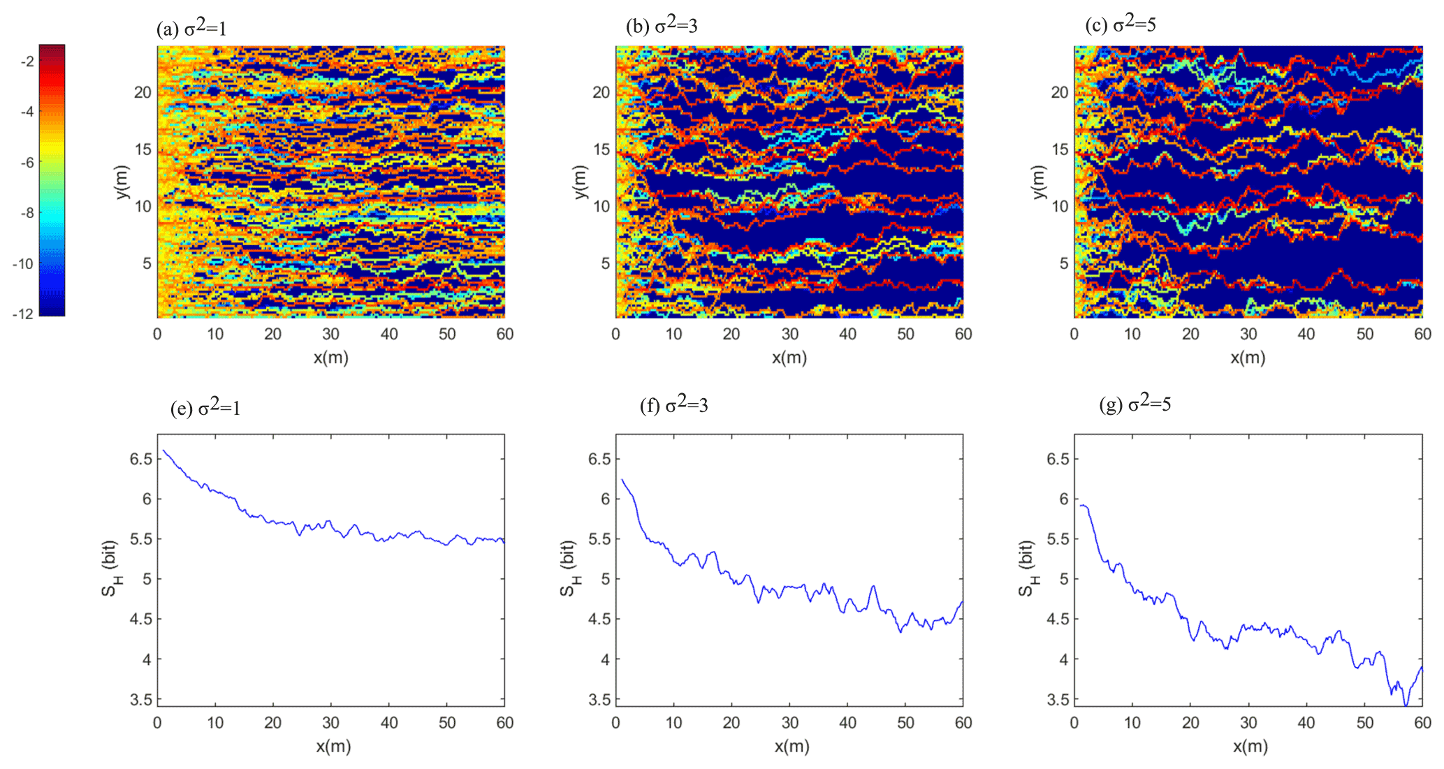
Figure 2 Accumulated, normalized number of particles that passed a distinct point in the domain as a function of the variance in ln(K), σ², (a, b, c) and the corresponding Shannon entropy of the transversal concentration, S_H, as a function of the main flow direction (d, e, f).

This reflects the increasing order in the flow path distribution, corresponding to the emerging and increasing transversal concentration gradients. A comparison of S_H among the variance cases clearly corroborates the visual impression that the number preferential flow paths declines with increasing randomness, while the concentration of solutes therein increases. The analysis of flow path entropy within the entire set of 100 realizations revealed that this behavior is not an artifact of single realization. The flow path entropy averaged across all realizations of a variance case exhibits a steady downstream decline (Fig. 3a, ΔH= 100 m). The curves are clearly shifted to lower values with increasing variance of ln(K), and the differences between the averages exceed the standard deviations within the ensembles. The boxplots in Fig. 3b (ΔH= 100 m) characterize the distribution of S_H(x) at the downstream outlet among the realizations. While the spreading and the skewness of the distribution clearly increase with increasing variance in ln(K), we also observe that flow path entropy at the outlet declines clearly and statistically significantly with increasing variance, as the differences between the medians exceed the confidence limits.

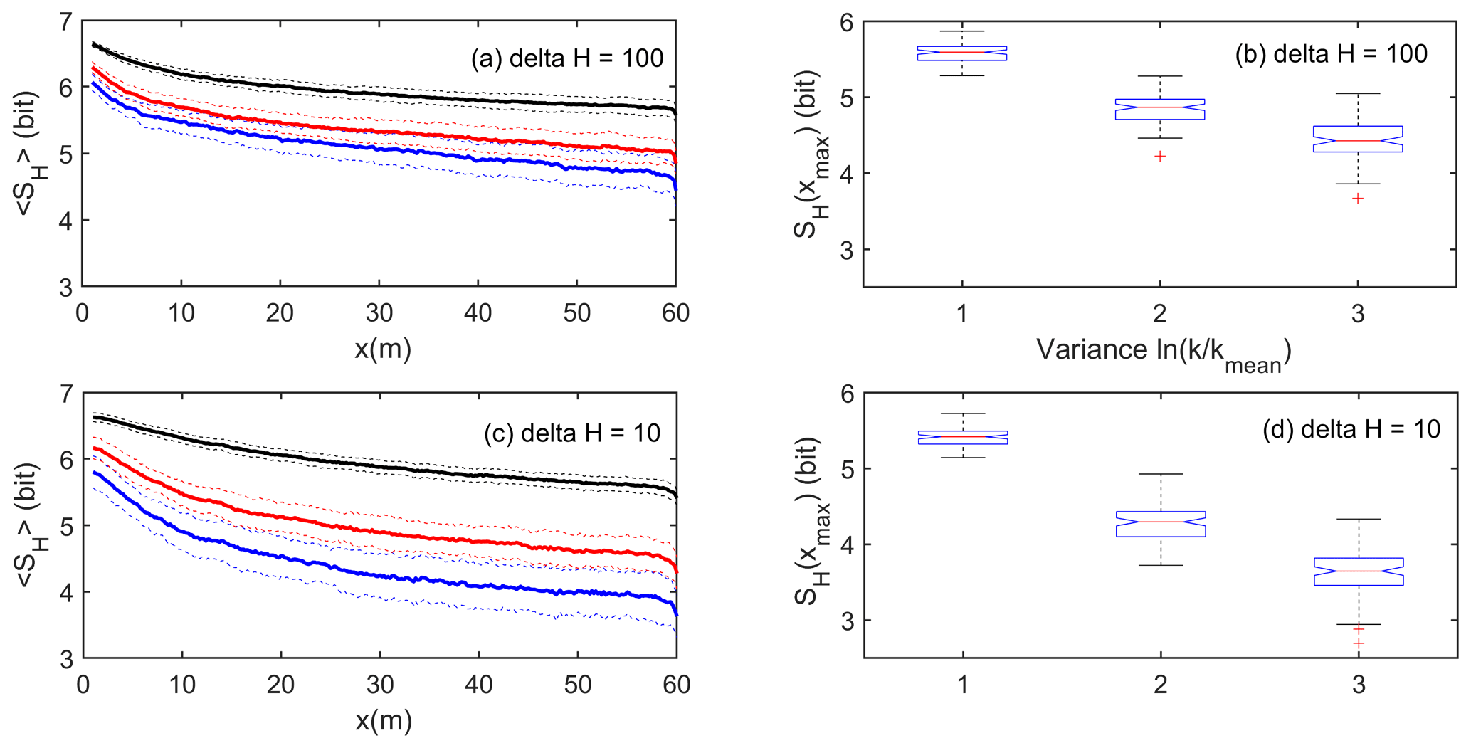
Figure 3 Flow path entropy averaged across all 100 ensemble realizations <S_H> as a function of downstream transport distance for (a) ΔH= 100 m and (b) ΔH= 10 m; the dashed lines mark the range plus/minus the standard deviations. Boxplot of flow path entropy at the domain outlet for all realizations of the three variance cases for (c) ΔH= 100 m and (d) ΔH= 10 m; note this corresponds to the asymptotic values in (a) at x= 60 m.

We thus state that a higher variance – and thus randomness – in hydraulic conductivity coincides, for all realizations, with a stronger downstream reduction of the flow path entropy. This corresponds to a macrostate of higher order due to a more efficient self-organization into a state of stronger preferential transport. In the case of the lower driving head difference of ΔH= 10 m, an even stronger self-organization manifests, as reflected in the smaller average flow path entropies for variances of σ²= 3 and 5, respectively (Fig. 3c and d).

4.2 Power in fluid flow as a function of the variance in ln(K)

Figure 4a–c compare the distribution of power in the fluid flow calculated according to Eq. (7), as a function of the variance of ln(K) in the different domains for the driving head difference of ΔH= 100 m. For consistency, we used the same ensemble as for Fig. 2. The distributions of power in the fluid generally spread across a wide range of magnitudes and are skewed to the left. However, the distributions clearly shift to larger values, and their spread becomes wider when moving to larger variances. This is underpinned when comparing the integrated power in fluid flow across the entire two-dimensional domain. An increase in variance by 4 orders of magnitude in the lognormal scale corresponds to an increase in power of 2.28 W per unit width of the domain. A closer look reveals that this increase in total power stems mainly from the increasing power in the vertical/transversal flow component (Fig. 4d–f). To further illuminate whether the above postulate of a strong linear relation between power and variation in the head gradient exists, we integrated power in fluid flow across the transversal extent of the domain ($P_{\mathrm{int}}^x$ hereafter) and plotted it against the laterally averaged head gradient (Fig. 3g–i). In the case of a unit variance, this indeed yields a strongly linear relation, with an almost perfectly linear growth of $P_{\mathrm{int}}^x$ with the head gradient, as indicated by the correlation coefficient of 0.96. While this correlation becomes weaker with increasing variance, it remains significant, even for the case of σ²= 5 with a correlation coefficient of r= 0.84. The decline in correlation is plausible as a higher variability in K in the two-dimensional domains causes stronger transversal flow components and thus a larger deviation from the one-dimensional heterogeneous case for which Eqs. (9)–(12) are valid. The increasing role of transversal flow is also reflected by the increasing power in the vertical flow component with increasing variance (Fig. 4d–f). As expected, the head gradients also show a wider spread with increasing variance (Fig. 4g–i); the same holds true for power in the total downstream fluid flow. For simulations driven with a head difference ΔH= 10 m, the correlation relation between downstream power and the local head gradient was even stronger, with values of r= 0.97, 0.94, and 0.91 for σ²= 1, 3, and 5, respectively.

To check the inverse-linear relationship between ln(P) and ln(K), which was derived for the one-dimensional approximation as well (recall Eqs. 11–13), we related ln($P_{\mathrm{int}}^x$) for ΔH= 100 m to the logarithm of laterally averaged conductivity ln(K_eff) (Fig. 4j–l). For the unit variance, we observe an almost perfect linear increase of ln($P_{\mathrm{int}}^x$) with a decline in ln(K_eff), as underpinned by the correlation coefficient of r= −0.92. This negative correlation declined with increasing variance to values of r= −0.81 and r= −0.72 for σ²= 3 and σ²= 5, respectively, yet they are still significant. For the lower head of ΔH= 10 m, the anti-correlation is stronger again, with r values of −0.93, −0.83, and −0.76, for σ²= 1, 3, and 5, respectively.

Figure 4 Histogram of log power ln(P) (a, b, c) and log power in the vertical water flux ln(P^z) (e, f, g) as a function of the variance σ². Integral power $P_{\mathrm{int}}^x$ in the total downstream water flux, plotted against the laterally averaged head gradient (g, h, i) and ln($P_{\mathrm{int}}^x$) as a function of the log of the transversally averaged K, ln(K_eff) (j, k, l).

We hence state that the system also behaves energetically in the case of the highest variance, largely similar to a heterogeneous one-dimensional system; this holds even truer in the case of a smaller driving head difference. The power required to maintain the driving head difference and fluid flow in steady state increases with increasing variance of the hydraulic conductivity field. Regions of high total power coincide with large positive deviations of the hydraulic head from its mean, which emerge in the vicinity of bottlenecks of low hydraulic conductivity. However, it is the increasing power in the vertical/transversal flow component that matters, as detailed in the next section.

4.3 Entropy as a function of work and power along solute transport trajectories

Figure 5 presents boxplots of the power in the vertical flow component P^z as a function of the variance in ln(K) for the head differences of ΔH= 100 and 10 m. These results confirm that it is indeed mainly the power in the vertical flow component that grows with increasing variance of K. This makes intuitive sense because transversal concentration gradients are formed by vertical flow and transport of solute particles.

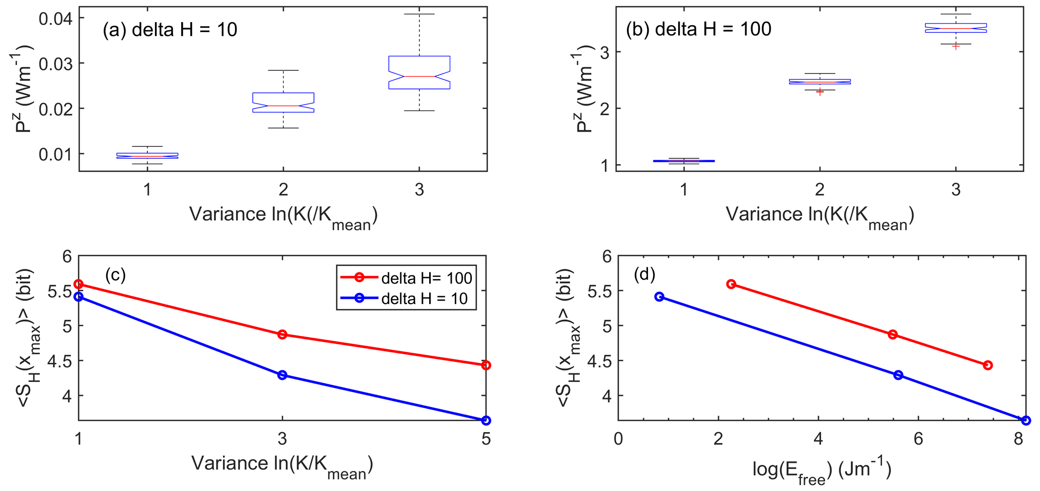
Figure 5 Boxplots of the power in the vertical flow component P^z as a function of the variance in ln(K) for the head difference (a) ΔH = 100 m and (b) ΔH= 10 m. The corresponding median flow path entropy of the ensembles at the domain outlet is plotted as a function of the variance of ln(K) (c) and against the median work E_free performed by the fluid. The latter is power times the maximum travel time to the outlet.

The growing power in the vertical flow component explains, hence, the stronger self-organization and declining flow path entropy with growing variance.

While the differences in vertical power P^z are significant between the variance cases, vertical power is in the case of ΔH= 10 m 2 orders of magnitude smaller than for the case of ΔH= 100 m. This is plausible as both the Darcy flow velocities and the local head gradients are on average 10 times smaller. The decline of the median entropy med(S_H(x_max)) with the med < P^Z > reveals, in line with the gas laser example given in the Introduction, that a larger power input due to a higher pumping rate leads to an higher order in the macroscale preferential transport pattern. Yet the reduction in flow path entropy at the domain outlet is stronger with increasing variance for ΔH= 10 m than for ΔH= 100 m (Fig. 5c). This is nevertheless plausible because the particle travel times in the case of ΔH= 10 m are between a factor of 10 to 100 larger (see also Fig. 7). Hence, this extra residence time (a) compensates for the on average 10 times smaller vertical flow velocities and (b) also implies that the work, defined as the integral of power in vertical flow along the particle travel times to the outlet, is larger for σ²= 3 and 5, as in the case of ΔH= 100 (Fig. 5d). The larger amount of work performed by the vertical flow component explains the stronger self-organization in the case of the lower head difference well.

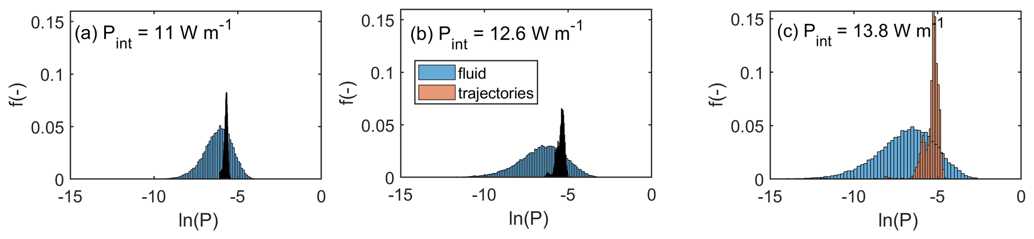
Figure 6 Cumulative distributions of ln(P) in the flow domain (blue) and of ln(P) averaged along the particle trajectories for (a) σ²= 1, (b) σ²= 3, and (c) σ²= 5.

Figure 6a, b, and c compare the probability density distributions (pdfs) of ln(P) within the entire flow domain (blue) against the power averaged along the actual particle trajectories (in brown). While in the case of perfectly mixed flow and transport, both pdfs should be rather similar, they actually are remarkably different. This is because particles accumulate downstream along pathways of high vertical power into preferential pathways, and this is clearly reflected by the shift of the pdfs towards higher power values.

4.4 Space–time asymmetry and entropy export into the breakthrough

To switch the observation perspective, we determined the particle breakthrough curves (BTCs) for the different variance cases and calculated their Shannon entropy as a means of uncertainty and order in the arrival times, using the time step width of 0.1 dimensionless time units as bin width. For the head difference ΔH= 100, the width of the breakthrough curves clearly increases with increasing variance, indicating an earlier breakthrough, a longer tailing, and a more even distribution of normalized concentrations in time (Fig. 7a). In the case ΔH= 10, we observe a similar but stronger behavior and a clear shift to larger breakthrough times, due to the smaller Darcy velocities (Fig. 7b). For both head differences, one can observe that the Shannon entropy in arrival times grows with increasing variance of ln(K), reflecting a larger uncertainty and a declining order in the temporal distribution of travel times. In this context, it is important to recall that entropy cannot be consumed, due to the second law. This that means that the declining flow path entropy needs to be exported from the system.

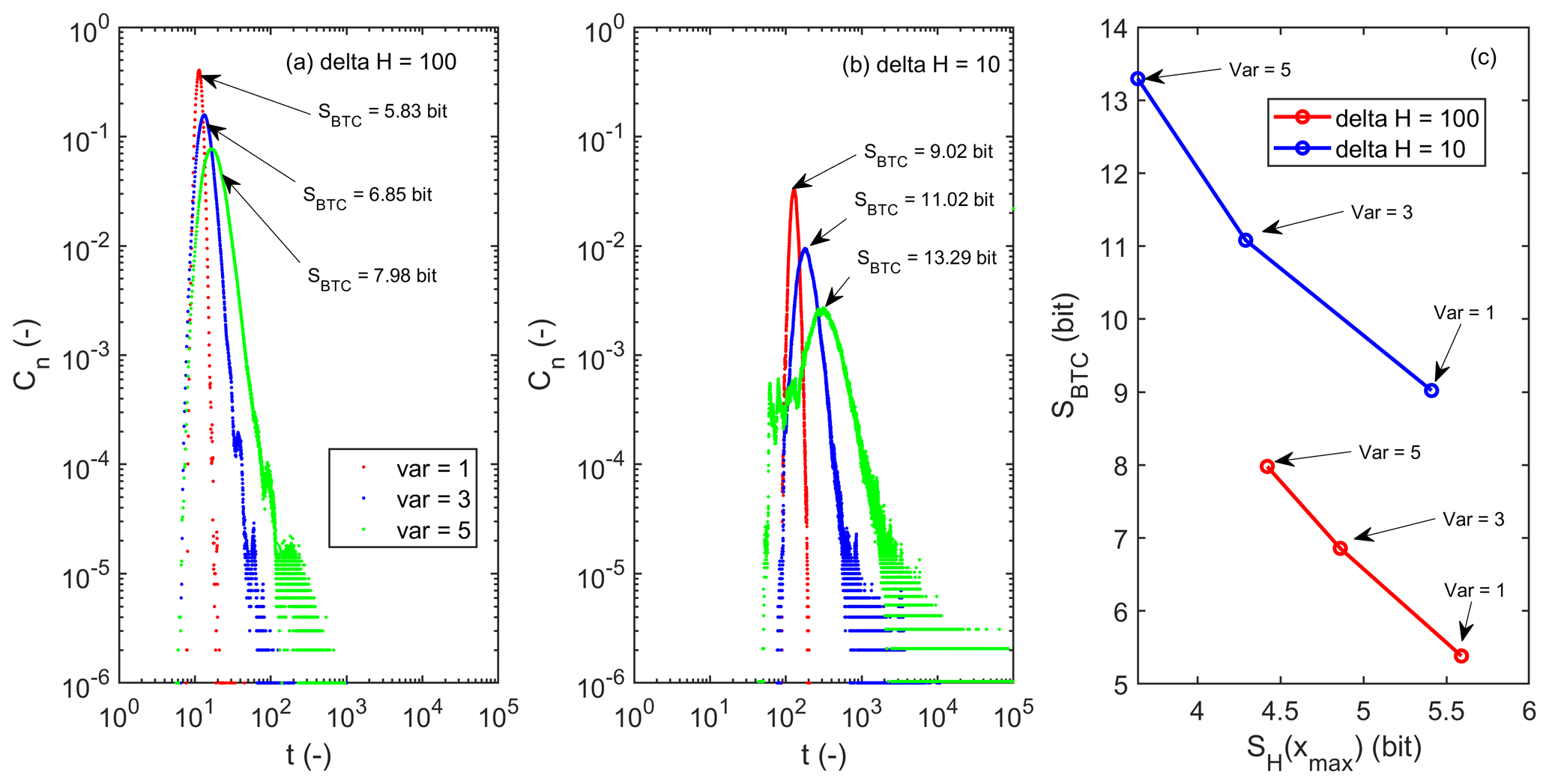
Figure 7 Breakthrough curves and their Shannon entropies S_BTC for (a) ΔH= 100 and (b) ΔH= 10. (c) S_BTC plotted against the flow path entropy of the downstream outlet S_H(x_max), before particles leave the domain, for all variance cases, and ΔH= 100 and 10, respectively.

Figure 7b clearly visualizes this space–time asymmetry in entropies; the growing spatial organization with increasing variance of ln(K) translates due to the associated entropy export into a declining organization in arrival times. Please note that due to the different binning in space and time, changes in S_BTC and S_H with changing variance cannot be exactly the same, in fact, also the entropy, which is produced due to energy dissipation. The opposite dependence of the BTC entropy on the variance in ln(K) corroborates nevertheless that the reduced flow path entropy is indeed exported into the BTC.

5 Discussion

5.1 An energy- and entropy-centered framework to characterize and explain preferential flow

This study proposes an alternative framework to quantify and explain the enigmatic emergence of preferential flow and transport in heterogeneous saturated porous media, using concepts from thermodynamics and information theory. We examined simulations of two-dimensional fluid flow and solute transport based on the methods of Edery et al. (2014), who at total head differences of 100 and 10 characterized the discrete probability distribution of solute particles to cross a distinct transversal position in a plane normal to the direction of the mean flow by means of the Shannon entropy. In general, we found a declining entropy with increasing downstream transport distance, reflecting a growing downstream self-organization due to the increasing concentration of particles in preferential flow paths. Strikingly, preferential flow patterns with lower entropies emerged when analyzing simulations in media with larger variances in hydraulic conductivity, and this enhanced self-organization appeared even stronger for simulations at lower head differences. This implies that macrostates of higher order are established, despite the higher randomness of ln(K) for a range of Péclet numbers representing strong and intermediate importance of advective transport. The key to explaining this almost paradoxical behavior is the finding that power in the vertical flow components grows with the variance of the hydraulic conductivity field. Due to this larger energy input, the vertical/transversal flow component may perform more work to increase the order in the flow path distribution, through steepening transversal concentration gradients as reflected in lower entropies.

Notwithstanding these findings, we of course recognize that the concepts of entropy, free energy, and work are, per se, not new in hydrology. We thus place our findings in context relative to related studies, in the sections below.

5.2 Measuring irreversibility and macroscale organization using the Shannon entropy

Here we show that the Shannon entropy of the transversal distribution of solutes is suited to quantify the downstream emergence of preferential solute movement, as reflected in a declining flow path entropy. Lower flow path entropies and thus a stronger spatial order in preferential transport are established when solutes are transported through stronger heterogeneous hydraulic conductivity fields. In this context, we recall that Edery et al. (2014) analyzed breakthrough curves using the continuous time domain random walk framework (Berkowitz et al., 2006). When fitting an inverse power law to the breakthrough curves, the corresponding β parameter (which is a measure of the degree of anomalous transport, with β increasing to 2, indicating Fickian transport) increased with increasing variance of ln(K). Here we analyzed the Shannon entropy of the breakthrough curves in time, and contrary to the flow path entropies, they grow with increasing variance of ln(K). This means that higher degrees in spatial order in solute transport that emerges at larger variances in ln(K), expressed by lower flow path entropies, translate into a higher entropy and thus a higher disorder and thus uncertainty in arrival times. This is reflected by an earlier first breakthrough, a retarded appearance of the peak concentration, a longer tailing in the breakthrough curves, and a higher similarity of the BTC to a uniform, rectangular pulse. This finding coincides well with the illustrative case that Bianchi and Pedretti (2017) used to compare solute breakthrough through ordered and disordered alluvial aquifers.

This space–time asymmetry in entropy and organization can, however, only be explained using the physical perspective of entropy and the second law. The emergence of spatially organized preferential transport and the related decline in flow path entropy essentially requires an export of the entropy from the system into the BTC. We thus conclude that the β parameter of the CTRW framework is also a twofold measure for spatial organization of solute transport through the system and temporal organization in arrival times and their asymmetry. One might hence wonder whether a perfect spatial organization due to preferential transport of the entire solute particles through a single preferential flow path would, in the case of a step input, translate into a BTC of maximum entropy/disorder, i.e., rectangular BTC (and vice versa). We return to this issue in Sect. 6.

We speculate, too, that the concepts of entropy, power, and work might be helpful to explore the interplay of dissolution and precipitation of minerals such as silicate or carbonate rock, and the related local feedbacks on saturated hydraulic conductivity, as investigated by Edery et al. (2021). These processes certainly affect and change the distribution of entropy and power in fluid flow. The key to assessing this is to include molar entropy and the free-energy differences associated with the chemical reactions and chemical energy fluxes associated with chemical transport into the entropy and energy balances.

5.3 Preferred flow and transport pathways as maximum power structures?

The idea that preferential flow coincides with a larger power in fluid flow has been discussed widely in hydrology. Howard (1971, cited in Howard, 1990) proposed that angles of river junctions are arranged in such way that they minimize stream power; later he postulated that the topology of river networks reflects an energetic optimum, formulated as a minimum in total energy dissipation in the network (Howard, 1990). This work inspired Rinaldo et al. (1996) to propose the concept of minimum energy expenditure as an enslavement principle for the self-organized development of river networks. Hergarten et al. (2014) transferred this concept to groundwater systems. They derived preferential flow paths that minimize the total energy dissipation at a given recharge, under the constraint of a given total porosity, and showed that these setups allowed for predictions of spring discharge at several locations. Minimum energy expenditure in the river network implies that power therein is maximized. In this light, Kleidon et al. (2013) showed that directed structural growth in the topology of connected river networks can be explained through a maximization of kinetic energy transfer to transported suspended sediments.

Our findings are in line with but a step beyond these studies, which commonly refer to preferential flow in connected, highly conductive networks. Here we find that solute particles prefer to move through pathways of very high vertical power, even when they are not connected by a continuous set of cells of relatively high hydraulic conductivity. On the contrary, these pathways incorporate regions of low hydraulic conductivity. This finding reflects the squared dependence of power on the spatial head gradient, which in turn becomes largest in regions of low hydraulic conductivity. We stress that this result, and our finding that a larger power input (due to a higher pumping rate) leads to a higher order in the macroscale preferential transport pattern, is a consequence of the imposed boundary condition. A steady-state head difference implies a positive energetic feedback: in a real-world experiment, the pump provides this feedback, as otherwise the gradient is depleted by the flowing fluid. Although such a positive feedback is straightforwardly established in a numerical model by assigning the desired constant head difference, it is important that this choice implies that such a positive feedback exists. Due to this virtual energy input, the vertical flow component and solutes may perform the necessary work to steepen the transversal concentrations and thereby establish an ordered preferential flow pattern at the macroscale. Ultimately, it is the higher necessary pumping rate/power and the duration of the experiment that determine the elevated total energy input into the domains with higher K variance. This constrains the amount of work performed by vertical flow components and explains (a) why preferential flow patterns of higher order emerge with growing subscale randomness and (b) why self-organization was even stronger in the case of a lower driving head difference of 10.

One might hence wonder whether an even stronger self-organization might be observed during similar simulations in 3D stochastic media. We generally expect similar behavior, because the local changes in power of the transversal flow component arise from the local feedback on the pressure head gradient upstream of the low-conductivity bottlenecks. The gradients steepen ahead of these bottlenecks, which implies a higher power in the transversal flow component. This feedback will also occur in a 3D confined system, as it is a direct result of the boundary conditions (no flow boundary conditions for the upper, lower, inlet, and outlet boundaries).

6 Conclusions and outlook

Based on the presented findings, we conclude that the combined use of free energy and entropy holds the key to characterizing and quantifying the self-organized emergence of preferential flow phenomena and to explaining the underlying cause of their emergence. Information entropy is an excellent, straightforward concept to diagnose self-organization in space and time: here, the formation of preferential transport is reflected in the downstream decline in the entropy of the transversal flow path distribution and in this decline becoming stronger with increasing variance of hydraulic conductivity. The concepts of free energy and physical entropy, however, provide the underlying cause: steepening of transversal concentration gradients requires work; the formation of even steeper gradients and lower flow path entropies needs even more work and thus a higher free-energy input into the open system. The higher necessary pumping rate and energy input into the domains is the reason why spatial organization in preferential solute movement increased with growing subscale randomness of hydraulic conductivity. This behavior is very much in line with what we discussed for the gas laser in the Introduction.

Entropy can, however, due to the second law not be consumed, and the declining flow path entropy is in fact exported from the system into the breakthrough curve. Shannon entropy allows again for the straightforward diagnosis, while physical entropy provides the reason for this space–time asymmetry in entropy, organization, and uncertainty. Transport of all solute particles through a single preferential flow path implied a maximum spatial organization and maximum knowledge certainty about the transversal spreading of solute. However, this would, due to the entropy export, result in a maximum disorder of and thus uncertainty about the arrival times, as the BTC would correspond to a rectangular pulse of uniform concentration. Advective diffusive transport through a homogeneous flow field implied, in the case of a spatially homogeneous step input, maximum uncertainty about transversal position of solute molecules, while the BTC would be perfectly certain and provide minimum uncertainty about arrival times. This space–time asymmetry in entropy implies that perfect organization and certainty about both flow paths and travel times can never simultaneously occur. This required consummation of entropy and thus violation of the second law of thermodynamics. However, we wonder whether effective predictions of the entropies in the BTC and the flow path distributions based on the knowledge driving head differences and the variance and correlation lengths of hydraulic conductivity might be achievable in the future. This will of course not tell us where solutes move and when they break through, but it will predict the related uncertainty as an important constraint of transversal distribution of transport pathways and travel times.