A hydrography upscaling method for scale-invariant parametrization of distributed hydrological models

Distributed hydrological models rely on hydrography data such as flow direction, river length, slope and width. For large-scale applications, many of these models still rely on a few flow direction datasets, which are often manually derived. We propose the Iterative Hydrography Upscaling (IHU) method to upscale high-resolution flow direction data to the typically coarser resolutions of distributed hydrological models. The IHU aims to preserve the upstream–downstream relationship of river structure, including basin boundaries, river meanders and confluences, in the D8 format, which is commonly used to describe river networks in models. Additionally, it derives representative sub-grid river length and slope parameters, which are required for resolution-independent model results. We derived the multi-resolution MERIT Hydro IHU dataset at resolutions of 30 arcsec (∼ 1 km), 5 arcmin (∼ 10 km) and 15 arcmin (∼ 30 km) by applying IHU to the recently published 3 arcsec MERIT Hydro data. Results indicate improved accuracy of IHU at all resolutions studied compared to other often-applied upscaling methods. Furthermore, we show that MERIT Hydro IHU minimizes the errors made in the timing and magnitude of simulated peak discharge throughout the Rhine basin compared to simulations at the native data resolutions. As the method is open source and fully automated, it can be applied to other high-resolution hydrography datasets to increase the accuracy and enhance the uptake of new datasets in distributed hydrological models in the future.

1 Introduction

Large-scale distributed hydrological and land surface models are used to provide estimates of available water resources (Schewe et al., 2014; Wada et al., 2014), flood risk (Hirabayashi et al., 2013; Ward et al., 2013), drought risk (Veldkamp et al., 2017; Wanders et al., 2015) and food production (Kummu et al., 2014), among other applications. These models contain a routing module to simulate streamflow, i.e., the lateral flow of water on the land surface. This is a key variable for understanding the water, energy and biogeochemical cycles and the effects of disturbances from anthropogenic climate change on these cycles (Wood et al., 2011).

The spatial pattern of average streamflow conditions is largely determined by the contributing area of a river segment (Quinn et al., 1991) which is imposed on a distributed model by its flow direction data, i.e., a rasterized representation of the river network. Simulated peak streamflow is particularly sensitive to the accuracy of the flow directions and river channel and floodplain parametrization (Paiva et al., 2011; Zhao et al., 2017) and very important at river confluences (Geertsema et al., 2018; Guse et al., 2020; Metin et al., 2020) and river outlets (Couasnon et al., 2020; Eilander et al., 2020a), where multiple fluvial and/or coastal flood drivers may combine to modulate a flood event. Furthermore, streamflow is the only measurable integral signal of basin response and is therefore widely used for model calibration (Beven, 2012; Bouaziz et al., 2021), underlining the importance of flow direction data in distributed hydrological models.

Over the last decade, large-scale distributed hydrological models have been applied at increasingly higher resolutions (Bierkens, 2015), which poses a challenge to the parametrization of these models to achieve similar model results independent of the spatial resolution (Samaniego et al., 2017; Wood et al., 2011). One particular challenge in this regard is the lack of adequate methods to scale hydrography data such as flow directions and river length and slope parameters (Imhoff et al., 2020). Furthermore, integrated models, such as hydro-ecological models (Lowe et al., 2006) or coupled hydrological–hydrodynamic flood models (Hoch et al., 2019), often require the representation of various processes at different spatial resolutions. This can be achieved by hydrological nesting of models but requires multi-resolution hydrography data for the seamless coupling of flow directions at the model domain boundaries.

Flow direction datasets are developed at a fixed, high-as-possible resolution and are typically described in the “deterministic eight neighbors” (D8) format, which sets the downstream direction of each cell to one of its eight neighboring cells. Well-known high-resolution (≤ 1 km) flow direction datasets include the 30 arcsec resolution HYDRO1k (U.S. Geological Survey, 2000) and the 3 arcsec resolution HydroSHEDS (Lehner et al., 2008) and MERIT Hydro (Yamazaki et al., 2019) datasets. These datasets are derived from hydrologically conditioned high-resolution elevation data based on the direction with the steepest slope (e.g., Lehner et al., 2008; Yamazaki et al., 2019). Unlike typical geospatial data, such as elevation, hydrography data cannot easily be scaled by spatial resampling techniques, and extensive data processing is required to change its spatial resolution (Lehner and Grill, 2013). Therefore, specialized automated upscaling methods to describe high-resolution flow directions and river parameters at coarser model resolutions (typically ≥ 1 km) are required to leverage these datasets for distributed hydrological modeling and to achieve seamless integrated multi-resolution modeling.

Several D8 flow direction upscaling methods have been developed (Döll and Lehner, 2002; Fekete et al., 2001; Olivera et al., 2002; Wu et al., 2011; Yamazaki et al., 2008), but none provides a fully automated open-source method that can easily be applied to high-resolution flow direction data. Most of these methods first determine which river segment to represent within each coarse-resolution cell and subsequently set the upscaled flow direction based on fine-resolution flow directions of that river segment. However, to determine which river to represent within a cell in order to preserve the river network often requires more information than contained in just one cell and its direct neighbors. For instance, the commonly used DDM30 dataset, which is used by most global hydrological models within the Inter-Sectoral Impact Model Intercomparison Project (https://www.isimip.org/, last access: 26 September 2021), requires manual corrections after an automated initial procedure to ensure the river network is well preserved (Döll and Lehner, 2002). To circumvent this problem the Flexible Location of Waterways (FLOW) method (Yamazaki et al., 2009) uses a format that allows a downstream cell to be located outside the eight direct neighbors. While effective, this format has not been used outside the CaMa-Flood model (Yamazaki et al., 2011) for which it was developed as most models are built to work with D8 data. The hierarchical dominant river tracing (DRT) algorithm (Wu et al., 2011) uses global information to order streams within a basin to determine which river segment to represent within a cell and reroutes rivers through neighboring cells if required. While DRT has proven successful at automatically upscaling 30 arcsec flow direction data to coarser resolutions (Wu et al., 2012), it has not been applied to higher-resolution data to the best of our knowledge, and its code is not available open source. Furthermore, none of the D8 upscaling methods derives both river length and slope sub-grid parameters, which are required by most hydrological models.

The first objective of this paper is therefore to develop a fully automated D8 flow direction upscaling algorithm in order to derive flow direction and representative river length and slope parameters that can be applied to high-resolution (< 1 km) global hydrography data. The second objective is to evaluate how the choice of upscaling method and resolution affects peak discharge simulation. The remainder of this paper is organized as follows: Sect. 2 describes the newly developed Iterative Hydrography Upscaling (IHU) method and the accompanying multi-resolution MERIT Hydro IHU dataset; Sect. 3 describes the benchmark and case study experiments; Sect. 4 presents the results of the benchmark of IHU at the global scale; Sect. 5 presents the results of a case study in which we test the resolution independence of simulated peak discharge; the results are discussed in Sect. 6, and conclusions based on this study are presented in Sect. 7.

2 The Iterative Hydrography Upscaling algorithm

Any flow direction upscaling method needs to determine which river segment to represent within each coarse-resolution cell. The Iterative Hydrography Upscaling (IHU) method balances between traditional upscaling methods that only use local information contained in one coarse-resolution cell and its direct neighbors (Döll and Lehner, 2002; Fekete et al., 2001; Olivera et al., 2002) and upscaling methods that use global information about the hierarchy of streams to determine which river to represent within each coarse-resolution cell (Wu et al., 2011). IHU makes a first estimate of the representative river for coarse-resolution cells but updates this estimate where it leads to errors in upstream–downstream relations between cells based on contextual information in an iterative process. This iterative approach, which makes use of contextual data, makes IHU effective and suitable for application to high-resolution hydrography data. Section 2.1 provides a step-by-step description of IHU; Sect. 2.2 describes how representative sub-grid river parameters are derived, and Sect. 2.3 discusses the upscaled MERIT Hydro IHU v1 dataset, which is released as part of this paper.

2.1 Flow direction upscaling

The IHU method is explained in this section and illustrated for a fictional river in Fig. 1, where the terminology used is explained in the legend. For convenience, we will henceforth refer to the target coarse-resolution raster cells as cells and fine-resolution raster cells as pixels. IHU requires an output cell resolution (dashed grey grid lines), which is a multiple of the input resolution, and two input maps: a fine-resolution flow direction map and upstream area map (blue lines, where darker blue indicates a larger river). The goal of the upscaling method is to define the most representative flow direction for each cell (arrows).

The IHU method comprises four iterations which all consist of three steps. The iterations are numbered and aimed at (row 1) initiating upscaled flow directions, (row 2) fixing erroneous flow directions, (row 3) optimizing the in-between outlet pixel distance and (row 4) minimizing the error made by erroneous flow directions. The steps of each iteration are lettered: (column A) initiate, (column B) analyze and (column C) update. Each step is explained in detail below and refers to a panel of Fig. 1. Iterations 2–4 can be repeated to improve the results.

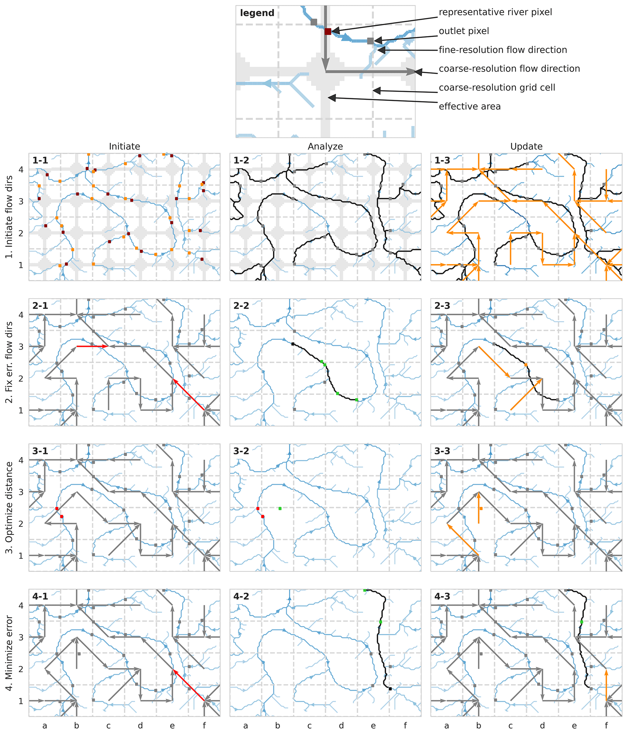
Figure 1 Illustration of the Iterative Hydrography Upscaling (IHU) method. Firstly, (1-1) the representative river pixel (dark red square) inside the effective area (shaded area) and the outlet pixel (orange square) are identified for each cell based on the upstream area; then (1-2) the fine-resolution flow path downstream of the outlet pixel (black lines) is traced to a neighboring cell to (1-3) set the initial upscaled flow direction (orange arrow). Secondly, (2-1) erroneous flow directions (red arrows) are identified and (2-2) analyzed in the context of the fine-resolution downstream flow-path (black line) with alternative outlet pixels (green squares) and tributary outlet pixels (grey squares) to (2-3) fix the flow directions by relocating outlet pixels (orange square and arrows). Thirdly, (3-1) outlet pixels with a short in-between distance are identified (red squares) and (3-2) alternative outlet pixels (green squares) with sufficient in-between distance are searched for, after which (3-3) outlet pixels are relocated and flow directions are updated accordingly (orange square and arrows). Fourthly, (4-1) remaining erroneous flow directions are identified (red arrows), and (4-2) from each neighboring cell the distance to a common downstream outlet pixel (green square) is measured to (4-3) update the flow directions (orange arrow) to the neighboring cell with the minimum distance in order to minimize upscaling errors.

• Step 1-1. The first iteration sets an initial flow direction for each cell. First, a representative river pixel is found for each cell (dark red square). This pixel is defined as the river pixel with the largest upstream area within the effective area (grey shade), as described by Eq. (1). Then, that pixel is traced downstream towards the outlet pixel (orange square), which is set as the most downstream pixel before leaving the cell. This first step of IHU builds on the effective area method (EAM) as it uses the same starting point to identify an initial representative river pixel per cell. By defining the effective area for selecting the representative river pixel in each cell, the method avoids selecting river segments that pass through only a corner of a cell and are unfavorable to determining flow directions (Paz et al., 2006).

  $$\begin{array}{}\text{(1)}& \left\{\left(x,y\right)\mathrm{|}\left({\left|x-x_{\mathrm{0}}\right|}^{\mathrm{0.5}}+{\left|y-y_{\mathrm{0}}\right|}^{\mathrm{0.5}}\right)<R^{\mathrm{0.5}}\right\},\end{array}$$

  where x,y gives the coordinates of a pixel; x₀,y₀ gives the coordinates of the center of a cell; and R is half the cell length.

• Step 1-2. The outlet pixel of each cell (grey square) is traced downstream (black lines) until an outlet pixel in a neighboring downstream cell is found. If no outlet pixel is found before leaving the eight neighboring cells, the trace is ended at the first pixel inside the effective area downstream of the outlet pixel, which is the default EAM procedure; see the trace downstream of the outlet pixel of cell b3 to cell c3 in the example.

• Step 1-3. The initial upscaled flow direction (orange arrows) is set for each cell in the direction of the cell where the trace in step 1-2 ends.

• Step 2-1. The second IHU iteration aims to conserve fine-resolution flow directions between outlet pixels at the coarse resolution, by repairing erroneous flow directions. The flow direction of a cell is erroneous if the first outlet pixel downstream is not located in its downstream cell (i.e., where the flow direction points to). In this step erroneous flow directions (red arrows) are identified. In the example, erroneous flow directions are found in cell b3 as the next downstream outlet pixel is found in cell d2 and not cell c3 and in cell f1 as the next downstream outlet pixel is found in cell e3 instead of cell e2. Steps 2-2 and 2-3 are then executed for each cell with erroneous flow directions, sorted from cells with a small to those with a large upstream area at the outlet pixel, and iterated until no more flow directions can be corrected.

• Step 2-2 (illustrated for cell b3 only). The outlet pixel of a cell with erroneous flow directions (black square) is traced downstream (black line) while potential alternative outlet pixels (green squares) are identified: these are defined as the last pixel before entering a new cell on the trace. The trace ends at the next downstream outlet pixel of a cell with correct flow directions and with only 1 potential outlet pixel. Cells directly upstream of cells with (alternative) outlet pixels on the trace are marked as tributary cells, and their outlet pixels are marked as tributary outlet pixels (grey squares). For all tributary cells the first and last alternative outlet pixels to which a valid flow direction can be set are identified. The erroneous flow directions are then updated based on the following iterative procedure.

  Starting from the most upstream outlet pixel on the trace, an outlet pixel is relocated to the most downstream alternative outlet pixel in a neighboring cell for which flow directions from the upstream and all tributary outlet pixels can be set correctly. If it is required to set the flow directions of tributary cells correctly, a tributary outlet pixel of a headwater cell (i.e., cells without upstream neighbors) can be relocated to an alternative outlet pixel. This is repeated until the end of the trace is reached.

  If at some point no valid alternative outlet pixel is found, the position of the last relocated outlet pixel is flagged as a bottleneck and not considered in the next iteration. Note that there are no bottlenecks in the example.

  This step is iterated until it is successful or until no new bottlenecks are found.

• Step 2-3. If step 2-2 is successful, the flow directions are updated accordingly. In this example the outlet pixel of cell c2 is relocated (from the black to orange square), thereby changing the flow direction for cell b3 and cell c1 (orange arrows). The first outlet pixel downstream of cell b3 is now located in cell c2 where the outlet pixel is relocated to the main stream. The first outlet pixel downstream of cell c1 is located in cell d2. Note that the flow direction of cell f1 cannot be repaired because two rivers flow parallel through its downstream cell e2, of which only one can be represented at the output resolution.

• Step 3-1. The third iteration aims to optimize the distance in between outlet pixels, measured along the fine-resolution flow directions. If this distance is short, 1 of the outlet pixels can potentially be removed in favor of another river segment within the same cell. A short in-between outlet pixel distance is not favorable when this distance is used to set the river segment length in routing models as it will decrease the accuracy or require smaller time steps. In this step, outlet pixels with an in-between outlet pixel distance smaller than a threshold value are flagged (red squares). This threshold is set to 25 % of the length of a cell edge, resulting in flagged outlet pixels for cell a2 and cell b2 in the example. Then, steps 3-2 and 3-3 are executed for every cell with a flagged outlet pixel until no more outlet pixels are relocated.

• Step 3-2. First, it is checked whether a flagged outlet pixel can be removed while the flow directions of its upstream neighboring cells can be set correctly. Then, alternative outlet pixels within the same cell are identified (green square). Alternative outlet pixels should have a minimum upstream area and a minimum distance to the next outlet pixel and may not be located downstream of any other outlet pixel. The minimum upstream area threshold is set to 25 % of the cell area to avoid creating cells with a small sub-grid area. In the example an alternative outlet pixel is found in cell a2.

  Step 3-3. If 1 or more alternative outlet pixels are found for a cell in step 3-2, the outlet pixel is relocated to the alternative outlet pixel with the largest upstream area, and the flow directions are updated accordingly. In the example the outlet pixel of cell a2 is relocated (orange square), thereby changing the flow direction for cell a2 and cell b2 (see orange arrows). The first outlet pixel downstream of cell a2 is now located in cell b2 because cell a2 now represents another stream. The first outlet pixel downstream of cell b2 is now located in cell b3 as the original downstream outlet pixel in cell a2 is relocated.

• Step 4-1. This iteration aims to minimize upscaling errors where erroneous flow directions cannot be repaired. This occurs mostly where multiple rivers flow parallel through the same cell and one can be represented in the D8 format. First, cells with remaining erroneous flow directions after step 2 are identified (red arrows). Then, step 4-2 and 4-3 are executed for each identified cell, sorted from cells with a large to cells with a small upstream area at the outlet pixel. In the example, the flow direction of cell f1 is erroneous as two rivers flow parallel through its downstream cell e2.

• Step 4-2. The fine-resolution path downstream of a cell with erroneous flow directions is traced (black line), and outlet pixels on the trace are identified (green squares). For each neighboring cell the coarse-resolution flow direction is followed until it reaches an outlet pixel on the trace. The distances to this outlet pixel from the neighboring cell and to this outlet pixel from the cell with erroneous flow directions are measured in number of outlet pixels and summed. This yields a combined distance to a common downstream outlet pixel for each neighboring cell. If multiple neighboring cells have the same combined distance, the cell with the largest upstream area at the outlet pixel is selected as a downstream pixel. Finally, if setting the flow direction to a neighboring cell causes the flow directions from two adjacent cells to cross, this cell is not considered. In the example, the combined distance from the pixel of cell f1 and neighboring cells e1, f2 and e2 to a common downstream outlet pixel is calculated.

  If no downstream outlet pixel is found on the trace and the last pixel of the trace is at a river mouth or sink, that pixel is set as the outlet pixel in the cell with erroneous flow directions if within two cells' distance. Note that in this case the outlet pixel is located outside the cell to which it belongs. If iterations 2–4 are repeated, this step is only executed in the last repeat. This situation occurs if a larger river flows through the cell with the river mouth or sink pixel. This step preserves secondary rivers in cells with larger rivers or multiple river outlets or sinks.

• Step 4-3. The flow direction is updated (orange arrows) to the neighboring cell with the shortest combined distance to a common downstream outlet pixel (green square). In the example the shortest combined distance from cell f1 to the common downstream outlet pixel in cell e3 is found in cell f2, changing the flow direction of cell f1 to cell f2 (north). While this introduces a small error into cell f2, the error is contained to just that cell, minimizing the upscaling error.

  The sensitivity of the R parameter to defining the effective area in step 1-1 as well as the minimum length and minimum upstream area thresholds used to optimize the sub-grid river length in step 3 is tested for the Rhine basin; see Appendix E. As steps 2–4 are iterated, the minimum river length and upstream area thresholds may also affect the upscaling accuracy as they may provide room for improvement in the next iteration of step 2. We found that the thresholds change the accuracy of the upscaled maps at less than 1 % of the output basin cells; see Fig. E1. A lower minimum upstream threshold generally has a positive effect on the upscaling accuracy and number of cells with a small river length but increases the number of cells with a small upstream area. The selected thresholds provide a balance between accuracy and cells with a small river length or contributing area, but if the latter is of less importance, the minimum upstream area threshold might thus be lowered for improved accuracy.

2.2 Sub-grid hydrography variables

Based on fine-resolution flow directions and so-called “outlet pixels”, several sub-grid variables are derived as shown in Fig. 2. The outlet pixel is the most downstream pixel of the representative river within each cell, see previous section, and used as a link between the coarse- and fine-resolution data.

• The sub-grid area is defined by the pixels draining to the outlet pixel of a cell and is confined by upstream outlet pixels; see Fig. 2b. This area is also referred to as the unit catchment area as introduced by Yamazaki et al. (2009).

• The river length is defined by the fine-resolution flow path found by tracing the outlet pixel of a cell either up- or downstream until the next outlet pixel; see Fig. 2c–d. When tracing a pixel upstream, the upstream pixel with the largest upstream area is selected in the case of multiple upstream pixels. The length is calculated along the sub-grid flow path based on the pixel size, with diagonal steps taken to be $\sqrt{\mathrm{2}}$ times the pixel size. Both up- and downstream river lengths are used in routing models and are derived here.

• The river slope is based on the MERIT Hydro elevation difference between 2 pixels at a set distance up- and downstream of the outlet pixel. Here we used a default distance of 2 km, 1 km up- and downstream of the outlet pixel. The flow path along which the slope is derived is shown in Fig. 2e.

• The river width is based on the MERIT Hydro width data layer at the outlet pixel. Note that these data contains gaps, see Fig. 2f, which show that not all outlet pixels (grey squares) have a river width (green colors) in the underlying data. For global coverage and application in hydrological models, these gaps need to be filled, which is outside the scope of this paper.

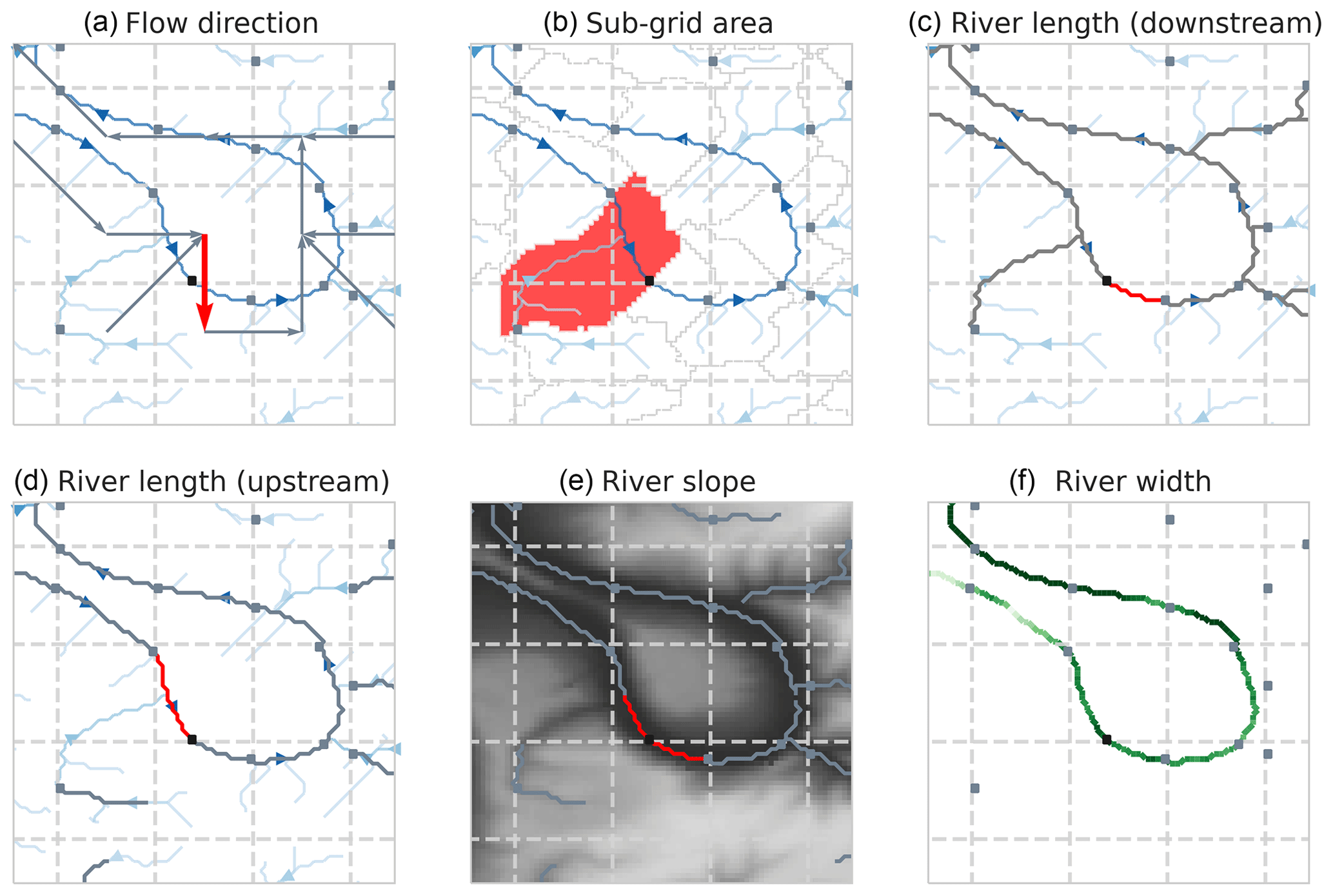
Figure 2 Output hydrography variables based on fine-resolution flow directions (blue lines in a–d; darker indicates larger upstream area) and/or outlet pixels (squares). Each variable is highlighted in red for the center cell and grey for other cells. The sub-grid area (b) is based on all pixels draining to the outlet pixel and limited by upstream outlet pixels. River length is derived based on the length of the flow path from outlet pixel to next downstream (c) or upstream (d) outlet pixel. The River slope (e) is calculated as the elevation (grey colors) difference over a flow path from a set length upstream to downstream of the outlet pixel. The river width (f) is derived based on the sub-grid river width (green colors) at the outlet pixel location.

2.3 Multi-resolution hydrography dataset

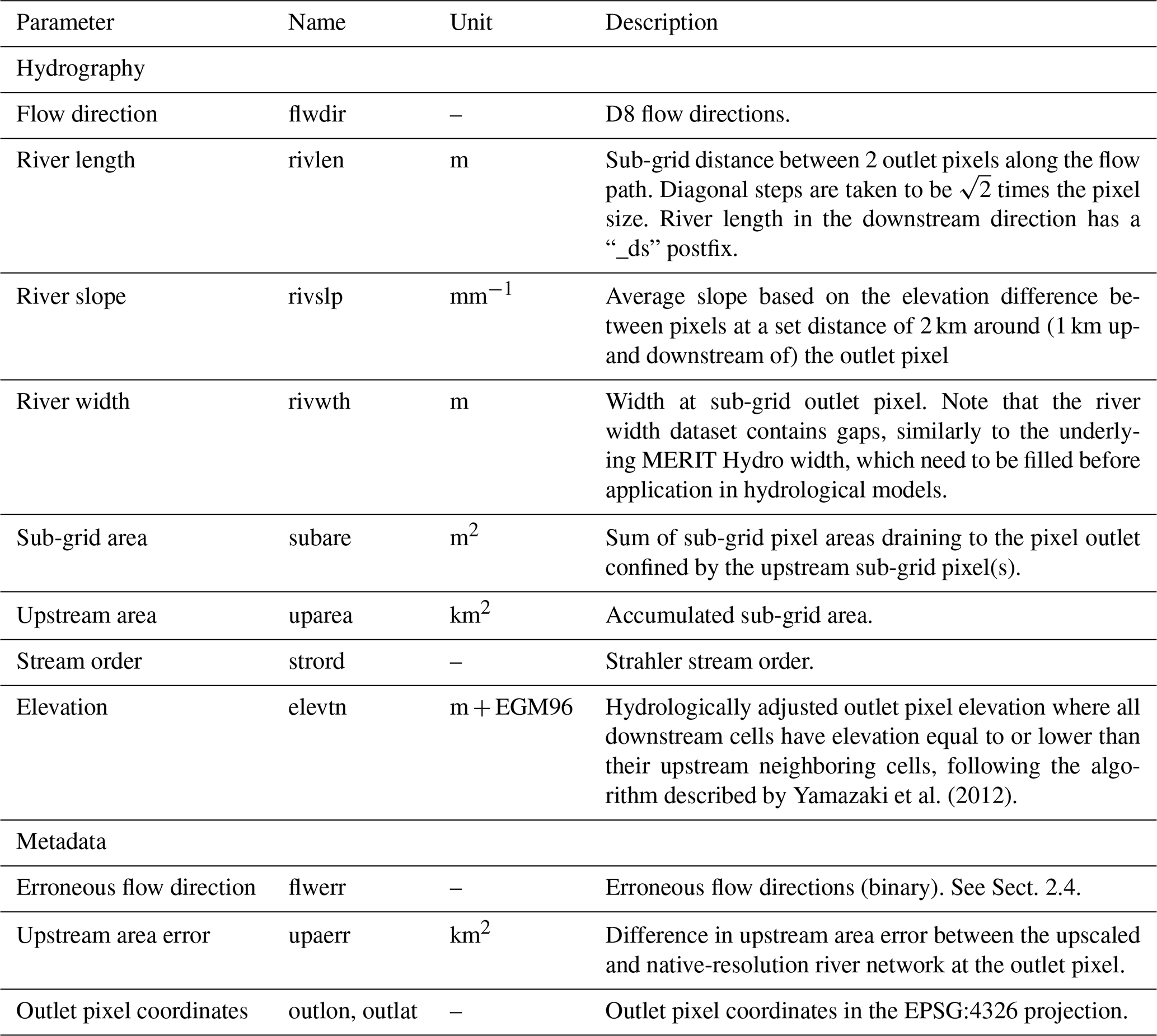
We derived the multi-resolution MERIT Hydro IHU dataset at resolutions of 30 arcsec (∼ 1 km), 5 arcmin (∼ 10 km) and 15 arcmin (∼ 30 km) by applying IHU to the recently published 3 arcsec MERIT Hydro data (Yamazaki et al., 2019). The original MERIT Hydro data were near-automatically derived based on the MERIT DEM (Yamazaki et al., 2017) and several water body datasets and show good agreement with drainage areas reported by the Global Runoff Data Centre (GRDC). We selected these MERIT Hydro data as they have a larger spatial coverage (90^∘ N to 60^∘ S) and better representation of small streams (Yamazaki et al., 2019) compared to earlier-published hydrography datasets. They also provide supplementary data layers including hydrologically adjusted elevation, which is used to derive the sub-grid river slope, and river channel width derived from the G1WBM permanent water body layer (Yamazaki et al., 2014), which in turn is used to derive the sub-grid river width. An overview of the layers in the upscaled MERIT Hydro IHU dataset is given in Table 1.

Table 1 Overview of hydrography and metadata layers of the MERIT Hydro IHU v1 dataset.

3 Methods

Besides IHU, see Sect. 2.1, we use the effective area method (EAM) (Yamazaki et al., 2008) and double maximum method (DMM) (Olivera et al., 2002) to perform benchmark and case study experiments. The DMM is selected as it is still often applied, for example in the recently published multi-scale routing model (Thober et al., 2019), and EAM is used as it is at the basis of the IHU method. For a full description of the methods we refer the reader to Appendix A as well as the referenced papers. In Sect. 3.1 we describe the implementation of upscaling algorithms and the application to the global MERIT Hydro dataset, in Sect. 3.2 the metrics used to evaluate the accuracy of the upscaling methods in a global benchmark, and in Sect. 3.3 the assessment of the effect of the upscaling method and resolution on simulated discharge for a case study of the Rhine basin.

3.1 Global application of flow direction upscaling methods

In this section we describe the application of the DMM, EAM and IHU algorithms on the global MERIT Hydro dataset (Yamazaki et al., 2019). All flow direction methods described in this section, including the DMM, EAM and IHU upscaling algorithms, are implemented in the open-source Python pyflwdir package (https://github.com/Deltares/pyflwdir, last access: 26 September 2021). For this paper pyflwdir v0.4.4 was used. For the reading and writing of the geospatial raster data we used the rasterio Python package (https://github.com/mapbox/rasterio, last access: 26 September 2021).

First some preprocessing was required to create a unique ID and delineate each basin. As we could not fit the entire global dataset into memory, an initial estimate based on the HydroBASINS dataset (https://hydrosheds.org/images/inpages/HydroBASINS_TechDoc_v1c.pdf, last access: 26 September 2021) was used. First, we assigned each outlet in the native-resolution MERIT Hydro dataset tile by tile to the nearest Pfafstetter level-2 HydroBASINS basin. We then used the bounding box of each Pfafstetter level-2 HydroBASINS basin to combine the MERIT Hydro data tiles and delineate the basins in the MERIT Hydro dataset. Within each Pfafstetter level-2 basin, all individual basins were numbered from the largest to smallest basin based on area to obtain a unique ID for each basin.

As the upscaling algorithms do not require information about the entire basin, the algorithms can be applied to each tile with sufficient overlap. We found that tiles of 10 by 10^∘ with a buffer of 10 times the target resolution provide consistent results. For each tile, the flow directions are upscaled; local flow direction errors (see next section) are calculated; sub-grid area, river length, slope and width variables are derived; and the native-resolution upstream area and basin values at the outlet pixels are read to assess the upscaling accuracy (see Sect. 3.2). After upscaling, the coarse-resolution data were again combined for each Pfafstetter level-2 basin to derive the upstream area, stream order and hydrologically adjusted elevation.

3.2 Upscaled flow direction accuracy metrics

We compute the following metrics at the global scale to benchmark the IHU against the DMM and EAM.

• Erroneous flow directions. The flow direction of a cell is erroneous if the first outlet pixel downstream of the outlet pixel of that cell is not located in its downstream cell (i.e., where the flow direction points to). Examples of erroneous flow directions are given by the red arrows in Fig. 1 panel 2-1. This measures the local accuracy of the upscaled flow directions, with fewer erroneous flow directions indicating a better representation of fine-resolution confluences at coarser resolutions.

• Upstream area error. The difference in upstream area between the target-resolution upstream area at cell $i\widehat{A_i}$ and the fine-resolution upstream area at the cells' outlet pixel A_i. This is an aggregated measure of the accuracy of all upstream flow directions. Based on the upstream area error we define Eq. (2), the absolute error ϵ; Eq. (3), the relative error ϵ_rel; and Eq. (4), the mean relative error $\stackrel{\mathrm{‾}}{{\mathit{ϵ}}_{\mathrm{rel}}}$:

  $$\begin{array}{}\text{(2)}& \mathit{ϵ}=\widehat{A_i}-A_i,\end{array}$$
  $$\begin{array}{}\text{(3)}& {\displaystyle }{\mathit{ϵ}}_{\mathrm{rel}}={\displaystyle \frac{\left|\widehat{A_i}-A_i\right|}{A_i}},\text{(4)}& {\displaystyle }\stackrel{\mathrm{‾}}{{\mathit{ϵ}}_{\mathrm{rel}}}={\displaystyle \frac{\mathrm{1}}{N}}{\sum }_{i=\mathrm{0}}^N{\displaystyle \frac{\left|\widehat{A_i}-A_i\right|}{A_i}}.\end{array}$$

3.3 Case study setup

For a case study of the Rhine in Europe, we assessed the effect of the resolution and upscaling method on simulated river discharge for a synthetic runoff event. For each method we calculated the difference in the simulated peak flow magnitude and timing between three upscaling methods at resolutions of 30 arcsec and 5 and 15 arcmin and a simulation based on the baseline 3 arcsec resolution. We expect smaller differences for IHU compared to other upscaling methods, especially at river confluences.

The Rhine basin catchment area up to the river outlet near Rotterdam, the Netherlands, has a surface area of approximately 195 000 km²; see Fig. 3. The basin has many smaller contributing sub-basins including the Meuse basin with its confluence near the river mouth after flowing parallel to the Rhine for many kilometers. Further upstream, the Moselle basin has many meanders, and in the upstream Swiss sub-basins many lakes are present. These features are typically hard to represent at coarser resolutions and therefore allow for a detailed benchmark between upscaling methods. Note that in reality the river flow in the Dutch part of the Rhine is more complicated than can be captured in D8 flow directions, with an important bifurcation, splitting the Rhine into the IJssel and Waal rivers and canals between the Waal and Meuse rivers.

The synthetic runoff event is assumed to be uniformly distributed throughout the Rhine basin. The runoff event is triangular shaped with a total duration of 10 d; it starts with 1.2 mm d⁻¹ and increases linearly to 6 mm d⁻¹ in 5 d after which it decreases back to 1.2 mm d⁻¹ in the next 5 d. This yields an initial flow of around 2700 m³ s⁻¹ and a peak discharge of around 10 800 m³ s⁻¹, which roughly correspond to average and 1-in-35-year discharge conditions respectively for the Rhine basin at Lobith (Hegnauer et al., 2014).

A routing model was set up to simulate channel flow for river cells, here defined as cells with a minimum upstream area of 10 km². By using this threshold, the area of headwater catchments, for which we assume instantaneous drainage, is more comparable between resolutions. Routing was based on a kinematic-wave-routing model, solved using the Newton–Raphson scheme as described in Te Chow et al. (1988) at a fixed time step of 15 min. Runoff of a headwater cell and within a river cell is instantly accumulated and fed to the channel at the outlet pixel of that cell. The channel length, slope and width at all resolutions are based on definitions in Sect. 2.2, where for the fine-resolution baseline data every pixel is considered to be an outlet pixel. A default length of 2 km around (1 km up- and downstream of) the outlet pixel was used to calculate the slope. To fill gaps in the river width observations, we fitted a power-law relation between the upstream area (A), as a proxy for the bank-full discharge, and MERIT Hydro river width (w) according to Eq. (5), where a and b are fitted to be 0.15 and 0.664 respectively; for more details see Appendix B, Fig. B1. Note that this is a simple approach that will not yield satisfying results if applied on a large scale or to actual events instead of as a sensitivity analysis based on a synthetic event.

$$\begin{array}{}\text{(5)}& w=a{A}^b\end{array}$$

In addition, we applied a default manning roughness coefficient of 0.03 and a minimum slope of 0.1 m km⁻¹. The default parameters are selected after a sensitivity analysis of the results to the channel slope length, width and roughness parameters; see Appendix F, Figs. F1–F2. While the simulated discharge peak magnitude and timing are sensitive to these parameters to varying degrees, they do not greatly affect the differences between methods and does not change the conclusions based on them.

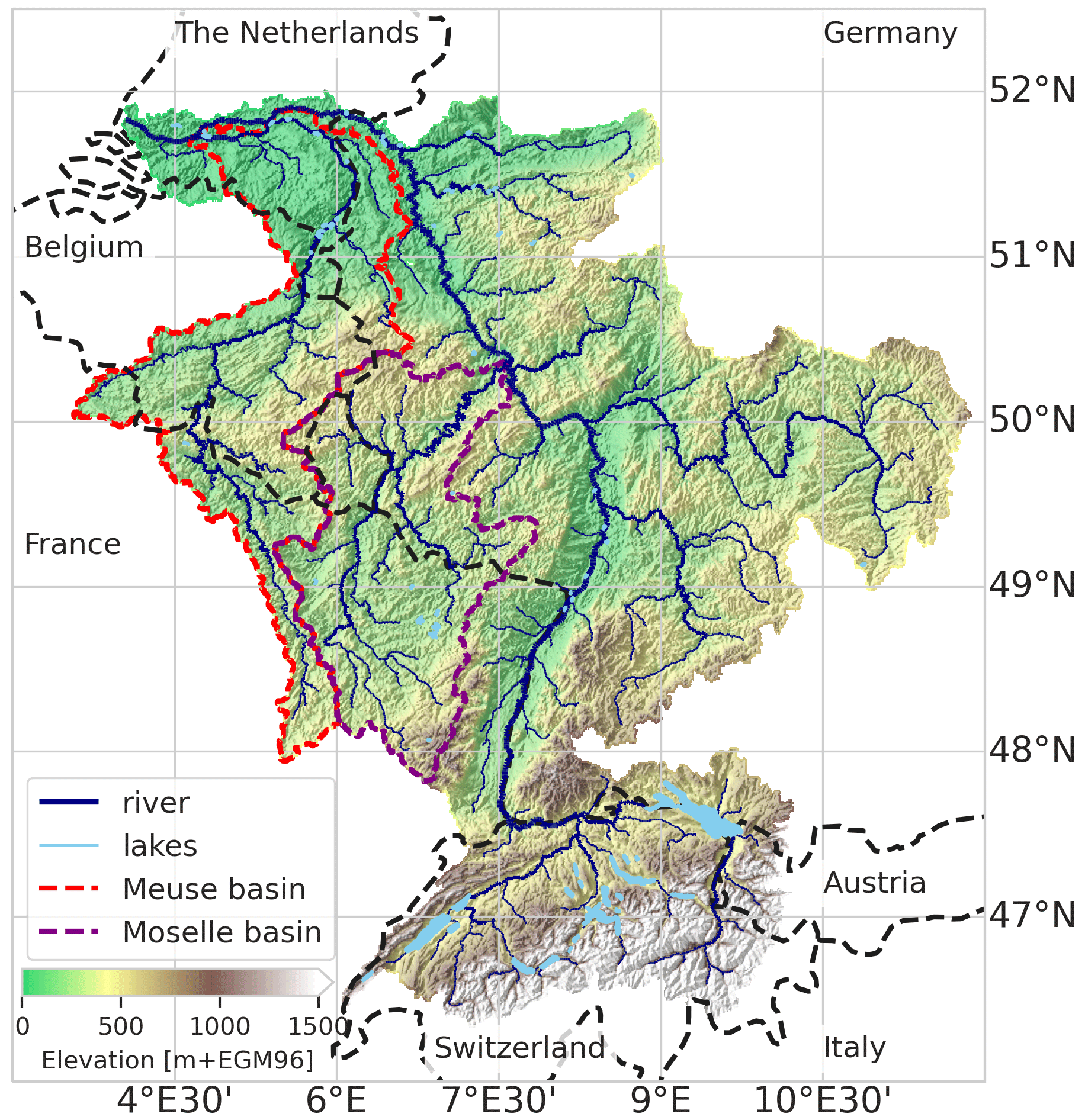
Figure 3 Study area. Rhine basin with average elevation, rivers and basin outlines based on the MERIT Hydro IHU 30 arcsec dataset (this paper); lakes are derived from the HydroLAKES dataset (Messager et al., 2016).

4 Accuracy of upscaling methods

In this section we benchmark the accuracy of IHU against the DMM and the EAM globally, based on erroneous flow directions and upstream area errors. Note that the results are presented at different spatial scales, from individual cells (Fig. 4) to basins (Table 2) and 1 by 1^∘ tiles (Fig. 5).

First, we analyze the percentage of native-resolution basins that are resolved in the upscaled flow direction maps. A basin is not resolved when it drains completely into neighboring basin(s) when upscaled and subsequently has no river outlet or pit at the coarser resolution. At each resolution we analyze the basins with a total area larger than approximately one cell. IHU resolves more than 96.2 % of the basins above the set thresholds compared to 85.7 % and 87.6 % for the DMM and EAM at a 30 arcsec resolution, while a larger percentage is resolved at coarser resolutions; see the first row in Table 2. Only two basins larger than 5000 km² are not resolved at the 15 arcmin resolution using IHU. These are an endorheic basin in the south of the Arabian Peninsula (6996 km²) and a small basin in Ontario, Canada (6830 km²); see Figs. C1–C2. Both are merged with a larger nearby basin as the river mouth or pits run through the same cell as the outlet or sink and they cannot be assigned to another neighboring cell. The largest unresolved basin at 5 arcmin has an area of 3521 km² and that at 30 arcsec an area of 40 km².

Next, we assess the percentage of cells with erroneous flow directions. This error is at the base of all upscaling errors discussed in this section and thus an important performance metric. The percentage of resolved basins that have fewer than 5% of cells with erroneous flow directions is above 92.2 % for IHU at all resolutions analyzed compared to 20.8 % for the DMM and 43.7 % for the EAM, see the third row in Table 2, indicating that many more confluences are properly resolved at the upscaled resolution. The difference between the methods is smaller for basins with fewer than 1 % of cells with erroneous flow directions. While the second iteration of IHU successfully limits this error compared to the DMM and EAM, the error cannot be avoided. For cells with parallel fine-resolution flow paths, it is impossible to correctly set the upscaled flow direction for all cells in the D8 format.

Table 2 Percentage of resolved basins with an area larger than approximately one cell that meet performance criteria based on relative basin area error, relative upstream area error (ϵ_rel) larger than 1 %, and cells with erroneous flow directions. For each criterion, the worst performance across all resolutions per method is highlighted with bold formatting.

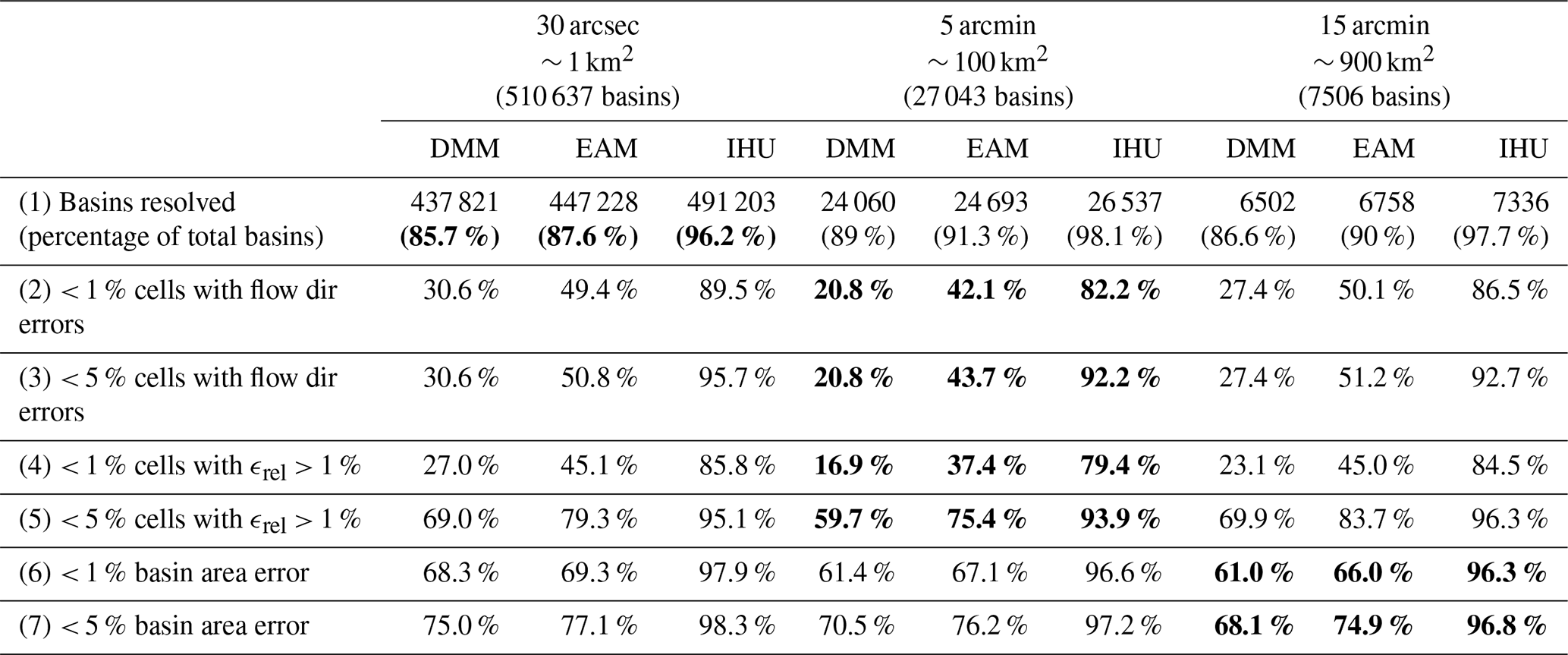
The relative upstream area error (ϵ_rel) considers the cumulative upstream error in erroneous flow directions. We find that more than 93.9 % of the resolved basins have fewer than 5 % of cells exceeding the 1 % upstream area error threshold for IHU compared to 59.7 % for the DMM and 75.4 % for the EAM; see the fifth row in Table 2. The difference between the methods is larger for basins which have fewer than 5 % of cells exceeding the 1 % upstream area error threshold. Figure 5 shows the percentage of cells within a 1-by-1^∘ tile with a relative upstream area error larger than 1 % for 5 arcmin resolution output maps. The differences between methods are consistent across the resolutions analyzed; see Figs. D1–D2. For IHU, most tiles have fewer than 1 % of cells with larger than a 1 % relative upstream area error. Exceptions are found in mountainous, glacierized and dry-land regions; see green areas in Fig. 5. For example, in dry-land areas such as the southern part of the Arabian Peninsula, northern part of Lake Eyre in Australia and some parts in the Sahara, where large rivers are absent, existing streams are ephemeral and flow directions extremely parallel; see for example Figs. C1 and C4. In regions covered by ice sheets such as Greenland, streams are not well depicted by the terrain elevation, based on which flow directions are estimated to be extremely parallel. In such areas, even at high resolutions, flow directions are highly uncertain.

The basin area error is analyzed based on the relative upstream area error at the basin outlet cell, as shown with dots in Fig. 5 for the 500 largest basins globally. For IHU more than 96.8 % of the resolved basins have a basin area error relative to original basin area of less than 5 % compared to 68.1 % for the DMM and 74.9 % for the EAM; see the seventh row in Table 2. This difference between the methods is larger with a basis area error of less than 1 %. While the fourth iteration of IHU, see Sect. 2.1, successfully limits this error in comparison to the DMM and EAM, it cannot completely be avoided. Large basin area errors of more than 10 % for basins larger than 1000 km² occur at 360 basins at a 15 arcmin resolution, 91 at a 5 arcmin resolution and zero at a 30 arcsec resolution. The largest basins with a 10 % basin area error at each resolution are shown in Figs. C3–C5. These errors occur when sections of basins are merged with neighboring basins because a cell from one basin becomes isolated between cells from another basin and none of the neighboring cells share a downstream outlet pixel.

The absolute upstream area error for all cells shows an improvement in performance for IHU compared to the DMM and EAM; see Fig. 4. While the error increases slightly with larger resolutions, it is consistently lower at all resolutions for IHU. At the 5 arcmin resolution 2.5 % of the cells have a positive upstream area error and 0.7 % a negative upstream area error compared to 9.9 % positive and 30.2 % negative for the DMM and 15.3 % positive and 5.8 % negative for the EAM. In general, the DMM shows a large percentage of negative upstream area errors, while the EAM and IHU tend to be skewed towards positive errors. Negative errors typically result from upscaled flow directions that cause a shortcut in a meandering section of a stream. The cells between the start and end of the shortcut then become a new branch in the upscaled flow direction map with a smaller upstream area. Both positive and negative errors occur when a confluence in the upscaled flow directions is erroneously located upstream of the actual confluence, thereby increasing the upstream area in one branch while decreasing it in the other branch where the number of cells with a positive or negative error depends on the length and the number of outlet pixels depends on each branch; see example in Fig. C6.

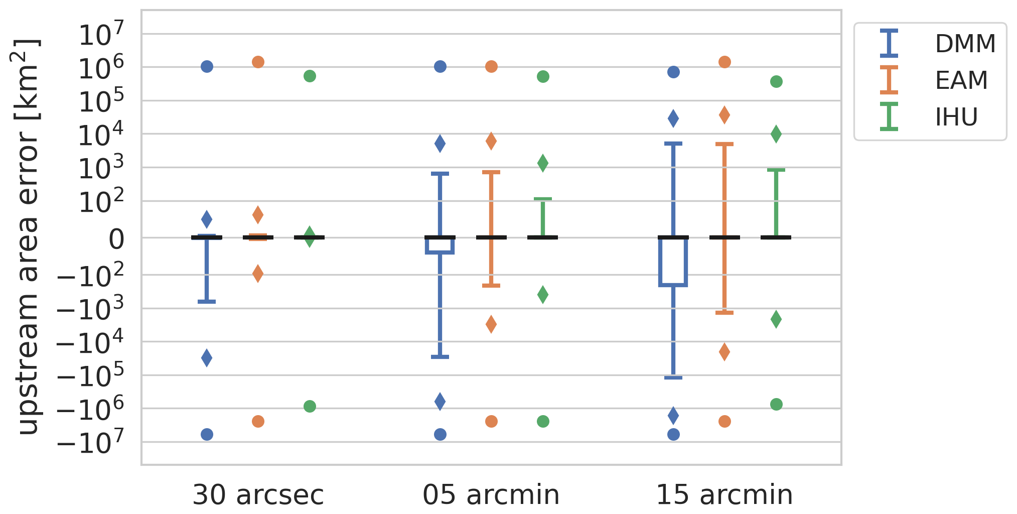
Figure 4 Absolute upstream area for the DMM (blue), the EAM (orange) and IHU (green) at three different resolutions from 30 arcsec (∼ 1 km; left column) to 15 arcmin (∼ 30 km; right column), where the black lines indicate the median error, the box the 25th–75th percentiles, the whiskers the 1st–99th percentiles, the diamonds the 0.1th–99.9th percentiles, and the dots the min and max errors.

Figure 5 Relative upstream area error (ϵ_rel at a 5 arcmin resolution (∼ 10 km)) for the DMM (a), the EAM (b) and IHU (c). The background colors show the percentage of cells per 1×1^∘ tile with a relative upstream area error of more than 1 %, while the markers show the relative upstream area error at the outlets or sinks of the 500 largest basins globally (black lines).

5 Effect of upscaling method on simulated discharge

In this section we assess the effect of the flow direction upscaling method on simulated discharge for a case study of the Rhine basin. First, we discuss the upscaled flow direction maps with the resulting upstream area error as shown in Fig. 6. Compared to the DMM and EAM, the upstream area error for the Rhine basin based on IHU is smaller (negligible at 30 arcsec) and more localized. A clear error that occurs at 5 and 15 arcmin resolutions with DMM and EAM is the erroneous confluence of the Meuse which is merged in the main stem upstream of the actual confluence; see Fig. 6. Furthermore, at the 30 arcsec and 5 arcmin resolutions many meanders in the Moselle basin are not correctly resolved with the DMM and EAM. For IHU at 15 arcmin a small error in the total basin area is made as a small stream near the outlet is erroneously merged into the Rhine basin, yielding a small error of 55 km² (0.02 %) at the outlet; see Fig. 6i.

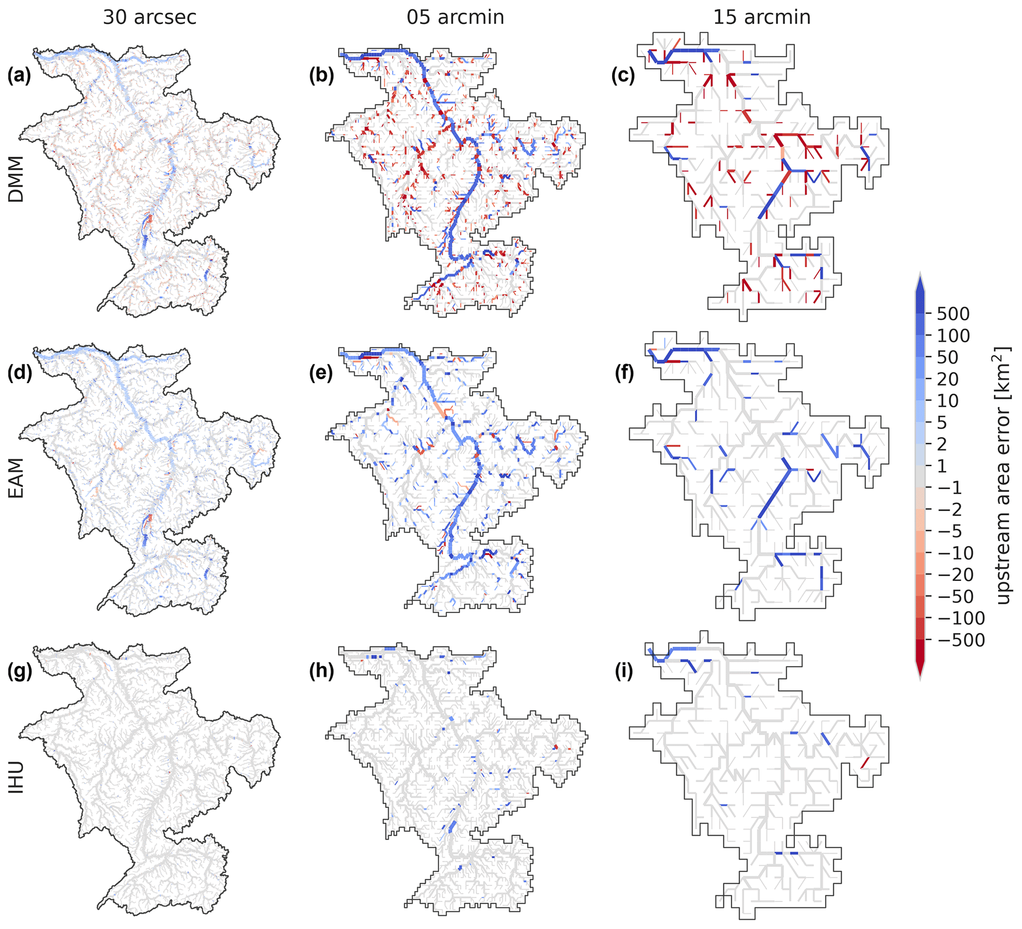
Figure 6 Upscaled MERIT Hydro flow direction network for the Rhine at resolutions of 30 arcsec (a, d, g), 5 arcmin (b, e, h) and 15 arcmin (c, f, i) as derived with the DMM (a–c), the EAM (d–f) and IHU (g–i), where red colors indicate a negative and blue colors a positive upstream error. The line thickness is scaled with the upstream area.

These flow direction maps together with the sub-grid drainage area and river map are used to set up a distributed routing model to simulate discharge as the result of a synthetic runoff event that is uniformly distributed throughout the catchment. We analyze the difference between simulated discharge in the upscaled model compared to the original 3 arcsec model. Figure 7 shows the runoff event (right y axis) and resulting flood peak wave at the river outlet (left y axis) for all methods and resolutions. It is immediately clear that models based on the EAM (orange) and IHU (green) perform much better, i.e., show better similarity to the model at the original 3 arcsec resolution, than the models based on the DMM (blue). The largest error in flood magnitude (+1024 m³ s⁻¹) and largest error in flood peak timing (−34 h) are found for the DMM at the 5 and 15 arcmin resolutions. These errors are likely due to a positive total area error in combining many shortcuts in the upscaled river network; see Fig. 6a–c. The largest errors in the flood peak magnitude for the EAM (−252 m³ s⁻¹) and IHU (−287 m³ s⁻¹) are found at the 15 arcmin resolution and the largest error in flood peak timing for the EAM (+1 h) and IHU (+2 h) are found at the 5 arcmin resolution. Both errors for both models have an opposite sign and are very small compared to models based on the DMM. While there are clear differences in the upstream area error between the EAM and IHU, see Fig. 6, the differences in simulated flood peak at the river outlet between the EAM and IHU are small. This is likely because the effect of upstream area errors on simulated discharge cancel out at the river outlet, see Fig. 6d–i, resulting in a net similar effect on the simulated discharge.

Figure 7 Simulated discharge at the river mouth of the Rhine near Rotterdam for a synthetic accumulated runoff event (grey line) and based on models with native 3 arcsec resolution flow directions (black line) in comparison to upscaled flow directions based on the DMM (blue; a), the EAM (orange; b) and IHU (green; c) at a 30 arcsec (dashed line), 5 arcmin (dash-dotted line) and 15 arcmin (dotted line) resolution. Note that the dimulated discharges for the 30 arcsec EAM and IHU runs largely overlap with that of the native 3 arcsec run.

To better understand the effect of flow direction upscaling on river routing, we therefore extend this numerical experiment to many locations across the Rhine basin; see Fig. 8. The locations are selected based on the outlet pixels at a 15 arcmin resolution that are at the same location as or near outlet pixels at a higher resolution. We use a maximum relative upstream area error of 1 % to select nearby outlet pixels at higher resolutions on the same stream, which results in 214 locations for the EAM compared to 343 for the DMM and 344 for IHU. The relatively small number of comparable locations for the EAM can be explained by the definition of the outlet pixels which are selected within the effective area rather than at the edge of a target cell and therefore are less likely to be the same between resolutions. Generally, simulated discharge based on the IHU upscaled river network yields smaller flood peak magnitude and timing differences compared to the DMM and EAM. In general, the IHU models show better similarity to the native-resolution model across the full distribution of locations for both flood peak magnitude and flood peak timing. The maximum relative difference in the flood peak magnitude between resolutions for 50 % (95 %) of the locations is smaller than or equal to 1.8 % (6.3 %) for IHU compared to 2.8 % (24.2 %) for the EAM and 14.2 % (98.5 %) for the DMM across all resolutions; see Fig. 8d. Similar results are found in terms of flood peak timing, where for 50 % (95 %) of the locations the maximum difference between resolutions is smaller than or equal to 2 (11) h for IHU, compared to 3 (13) h for the EAM and 5 (29) h for the DMM; see Fig. 8h. The differences in simulated discharge are caused by (local) upscaling errors in the river network. In both the DMM and EAM low-resolution river networks, the Meuse (most downstream and largest tributary with a size of about 16 % of the total basin) is merged into the main stem upstream of the actual confluence, causing large differences in both flood peak timing and flood peak magnitude in the Meuse section downstream of the erroneous confluence; see Fig. 8a–b and e–f. Not only are differences in flood peak simulations between upscaled and native-resolution models due to upscaling errors, also the upscaling of river width and slope is crucial for scale-invariant discharge simulations. For instance, differences in river width between resolutions in the upstream part of the Rhine basin cause a double peak at high resolutions (≤ 30 arcsec) to smoothen out into a single peak at lower resolutions, yielding relatively large differences in flood peak timing; see Fig. 8f and g. In the model, lakes and reservoirs are implicitly represented by larger channel widths from the MERIT Hydro dataset, introducing a buffering capacity in the river system. As the river width at lower resolutions is represented by the width at the outlet pixel of each cell, the buffering capacity is different. Averaging the river width would change the buffering capacity as this results in a smoothened river width. The sensitivity of the simulated flood peak timing to river width is shown in the first row of Fig. F2, where simulated river width is used for gaps in the river width data only (default), for lakes and data gaps, or for all cells (for details see Appendix B). Using simulated river widths at lakes and reservoirs minimized the timing error in the (upstream) Rhine. Besides width, the error in flood peak timing is also sensitive to the length along which the river slope is calculated; see Fig. F2. If this length is varied with the model resolution, large errors in flood peak timing are introduced. However, the flood peak timing error is less sensitive to the precise length within a range of 1 to 5 km.

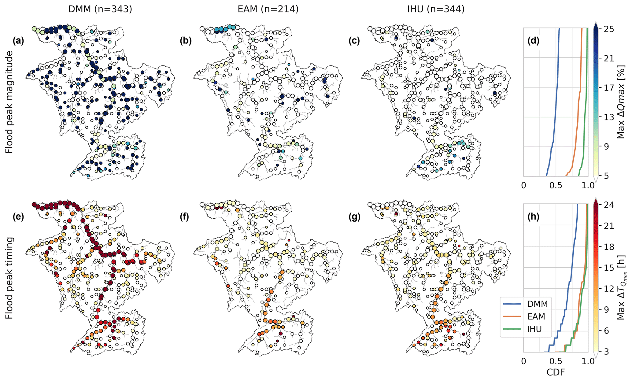
Figure 8 Maximum absolute difference in simulated flood peak magnitude (ΔQ_max – top row) and flood peak timing ($\mathrm{\Delta }{T}_{{\mathrm{Q}}_{\max }}$ – bottom row) between upscaled (30 arcsec, 5 and 15 arcmin) and the baseline (3 arcsec) resolutions in the Rhine basin based on the DMM (first column), the EAM (second column) and IHU (third column) upscaling methods. The right-most panels show the cumulative distribution function (CDF) curve for each method, with N denoting the number of comparable outlet pixel locations across all resolutions which are selected based on a maximum 1 % upstream area difference. The marker size is scaled with the upstream area, and markers are plotted in order of increasing upstream area.

6 Discussion

The proposed IHU upscaling method was shown to successfully upscale flow direction data from 3 arcsec data to resolutions up to 15 arcmin. IHU balances between traditional methods such as the DMM and EAM which only use local information and DRT which uses global information about the hierarchy of streams to determine which sub-grid stream to represent in each cell. IHU makes a first estimate of the representative sub-grid stream but updates this for cells with erroneous flow directions based on contextual information. This makes IHU more suitable to being applied to high-resolution hydrography data.

Compared to the EAM and DMM, flow directions are better resolved, specifically near confluences. This is important for correctly modeling flood peak propagation downstream of confluences, especially when flood peaks in nearby (sub-)basins are correlated (Berghuijs et al., 2019). Although much less compared to the EAM and DMM, erroneous IHU upscaled flow directions are still found in dry-land and ice-covered areas where the actual flow directions are also highly uncertain. These upscaling errors are mainly caused by many parallel flow paths in the fine-resolution hydrography data. This is partly a limitation inherent to the D8 format, which cannot represent multiple rivers that run parallel through a cell, making it impossible to upscale flow direction data without any errors. While a large majority of the basins have very small total area errors up to a 15 arcmin resolution if upscaled with IHU, the small number of large basins with a more than 10 % area error does increase with decreasing resolution. The exact upper limit of tolerable upscaling errors and thus the upscaling resolution depends on its application and region of interest. We believe that the 15 arcmin maps are suitable for many global-scale applications, but results in reported areas with lower accuracy should be interpreted carefully. To guide the user on the quality of the upscaled MERIT Hydro IHU dataset, we therefore provide qualitative metadata of erroneous flow directions and upstream area error. The DRT method by Wu et al. (2011) tries to solve the parallel flow path issue by allowing for rivers to be diverted through adjacent cells in favor of smaller rivers within that cell. Potentially, a stepwise upscaling procedure would even better preserve the largest basins and could be an interesting avenue for further research.

Besides flow directions, IHU derives additional layers of the sub-grid drainage area, river length and slope data, river width estimates for large rivers, and hydrologically adjusted elevation. While these layers cover most parameters required in the routing modules of many hydrological models, for a complete river parameter dataset a full-coverage river width layer is required as well as riverbed roughness. For more advanced routing models a riverbed level and river bank-full depth might also be required (Yamazaki et al., 2011). Several studies have shown that it is very hard to calculate reliable riverbed slopes from global DEMs (LeFavour and Alsdorf, 2005), while river routing based on a kinematic wave solution, as commonly used in large-scale hydrological models, is very sensitive to the river slope (Thober et al., 2019; Yamazaki et al., 2011). We found that a constant length across all resolutions of at least 1 km (500 m up- and downstream of the outlet pixels) is required to provide a relatively scale-invariant estimate of river slope as applied in the case study; see Figs. F1–F2. To achieve complete coverage of river width, the sub-grid river width data must be interpolated for data gaps and lake and reservoir areas if these are to be modeled explicitly in the routing model. Here, we used a strongly simplified power-law relationship between width and upstream area. For applications to real events instead of a sensitivity analysis with synthetic data, this estimate should be improved using the well-established geomorphic relationships between bank-full discharge and river depth as proposed in the downstream hydraulic geometry framework (Leopold and Maddock, 1953; Savenije, 2003), for instance by the clustering approach proposed by Andreadis et al. (2013) or with additional river width data from, e.g., Allen and Pavelsky (2018).

In this study we benchmarked several upscaling methods based on the same baseline hydrography data. This choice was made to focus the paper on differences in upscaling methods, where we assume the underlying high-resolution data are correct. For future studies it would be interesting to also compare the MERIT Hydro IHU dataset with often used hydrography datasets such as HydroSHEDS (Lehner et al., 2008) and HYDRO1k (U.S. Geological Survey, 2000), in terms of both the accuracy of the river network and the effect on simulated discharge for actual events.

Most multi-resolution routing models use data at preprocessed resolutions (Li et al., 2013; Wu et al., 2014; Yamazaki et al., 2011). However, Thober et al. (2019) recently presented a multi-scale routing model that includes the upscaling of flow direction data based on the DMM. Based on the presented results, using a multi-resolution modeling approach with hydrography based on IHU would likely improve the model's capability to simulate similar fluxes independent of the model resolution in studies like Imhoff et al. (2020). Furthermore, using a hydrological nesting approach, the model resolution could be varied within the model domain to add resolution where required for a correct representation of specific processes.

7 Conclusions

To describe flow directions and sub-grid river parameters in distributed hydrological models of different resolutions based on hydrography datasets with increasingly higher resolutions, automatic upscaling methods are required. The Iterative Hydrography Upscaling (IHU) method takes high-resolution flow direction data and upstream area data as input to derive flow directions at a coarser resolution while preserving the river structure. IHU was successfully applied to the 3 arcsec MERIT Hydro dataset to derive the MERIT Hydro IHU multi-resolution hydrography dataset at resolutions of 30 arcsec (∼ 1 km), 5 arcmin (∼ 10 km) and 15 arcmin (∼ 30 km). Additional layers of the sub-grid drainage area, river length, slope and width parameters are derived based on fine-resolution elevation and river width data.

Compared to other often-used upscaling methods, upscaled flow direction maps with IHU show improved accuracy for all metrics presented globally. For a case study of the Rhine basin we show that using IHU-based hydrography maps allows the use of lower-resolution routing models with similar results for the entire basin. Besides the upscaled flow direction data, the model similarity is also sensitive to how sub-grid river slope and width variables are derived. Because IHU is completely automated and yet accurate, it allows for a rapid uptake of new high-resolution flow direction data in distributed hydrological models at different resolutions.

Appendix A: Upscaling methods used for benchmarking

The EAM, the DMM and IHU have three steps in common. First, a pixel is selected for every cell that determines the representative river within the cell. Second, the pixel is traced downstream until a certain criterion in a neighboring cell is met. Third, the upscaled flow direction is set towards that neighboring cell. The differences between the methods are based on how the first two steps are implemented. The DMM and EAM are illustrated in Fig. A1 and briefly described below; more detailed descriptions can be found in the papers referenced.

A1 Double maximum method

• Step 1-1. The outlet pixel is defined as the pixel with the largest upstream area that is a basin outlet pixel either within the cell or located at the edge of the cell (grey squares).

• Step 1-2. The cell is offset by half the cell size in the direction of the cell quadrant in which the outlet pixel is found (dashed grid lines). The outlet pixel is then traced downstream until it leaves the offset cell (black lines).

• Step 1-3. The upscaled flow direction is set to the cell where the trace in step 1-2 ends (orange arrows).

  For a detailed description of the method we refer to Olivera et al. (2002).

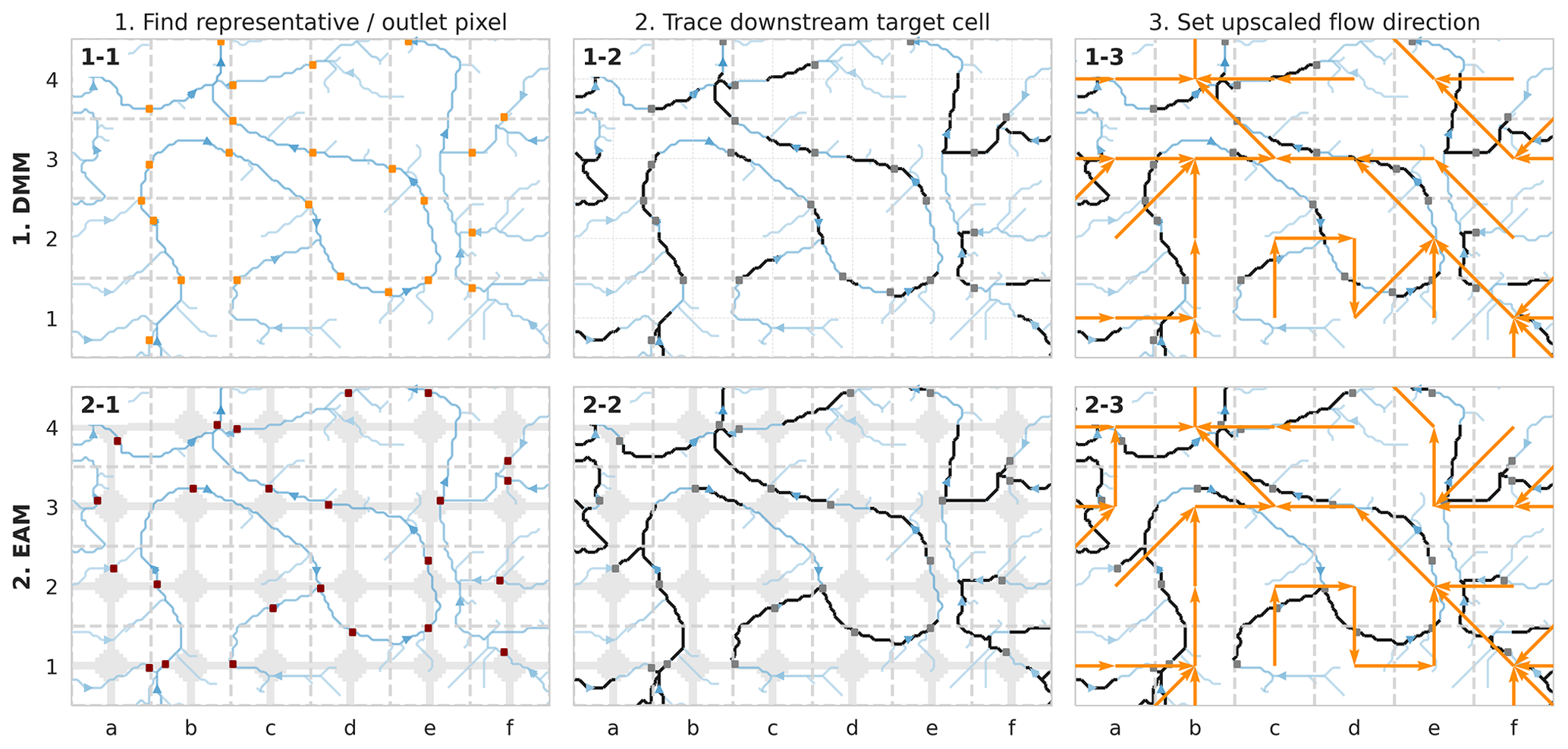
Figure A1 Visual explanation of the double maximum method (DMM; first row) and effective area method (EAM; second row). The target-resolution grid (grey lines) and fine-resolution upstream area map (blue colors) are shown in all plots. The representative (EAM) or outlet (DMM) pixels (squares) are traced downstream until a criterion in a neighboring cell is met (black lines), and the upscaled flow directions are set (orange arrows).

A2 Effective area method

• Step 2-1. The representative pixel (dark red squares) is defined as the pixel with the largest upstream area which is located within the effective area (shaded area) defined by Eq. (1); see Sect. 2.1.

• Step 2-2. The representative pixel is then traced until the first downstream effective area is reached, which by definition is in a neighboring cell (black lines).

• Step 2-3. The upscaled flow direction is set to the cell where the trace in step 2-2 ends (orange arrows).

  For a detailed description of the method we refer to Yamazaki et al. (2008).

Appendix B: River width interpolation

To fill gaps in the river width observations, we fitted a power-law relation between the upstream area (A), as a proxy for bank-full discharge, and MERIT Hydro river width (w); see Eq. (4). The MERIT Hydro river width was taken for all river cells within the Rhine catchment excluding cells within lakes and reservoirs based on footprints from the HydroLAKES (Messager et al., 2016) and GRanD (Lehner et al., 2011) databases. We used a least-squares error fitting algorithm from the Python scipy.optimize package (Virtanen et al., 2020) which was iteratively fitted to the sample after removing outliers based on the best fit. Outliers are defined based on the difference between the observed and simulated width of at least 200 m (for small widths) and the simulated width (for widths larger than 100 m).

Figure B1 Fitted relationship between the river width and upstream area for the Rhine basin.

Appendix C: Examples of upscaling errors

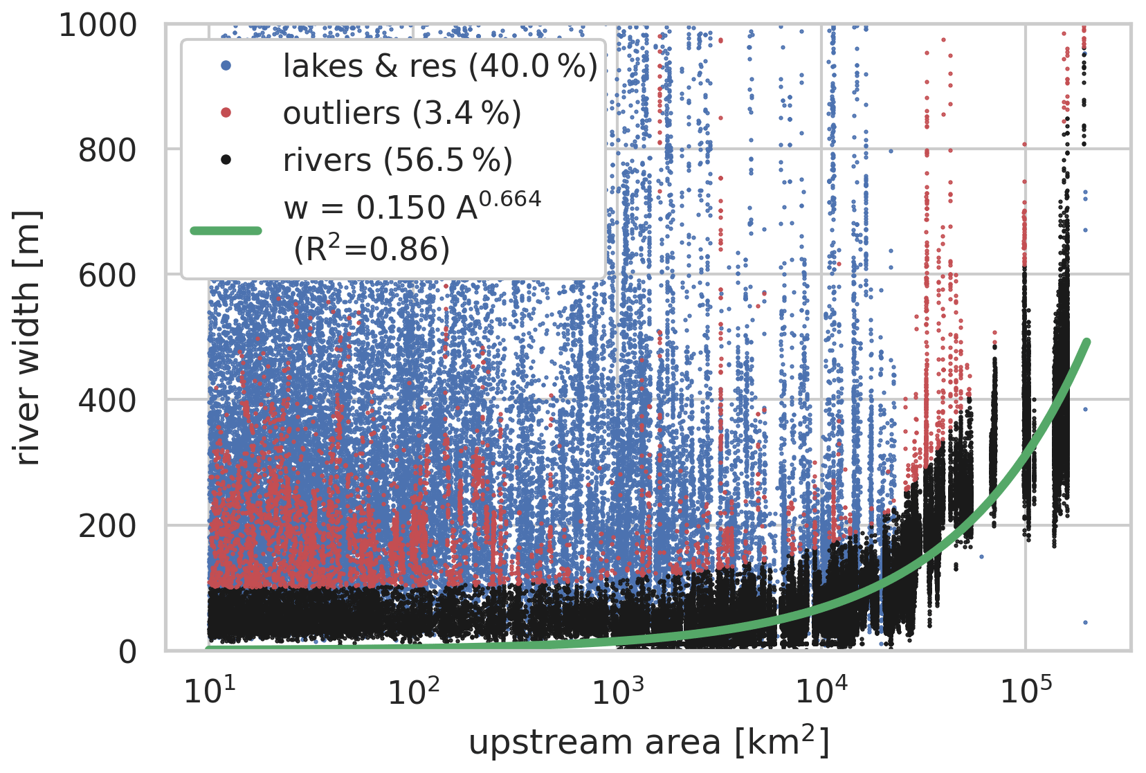
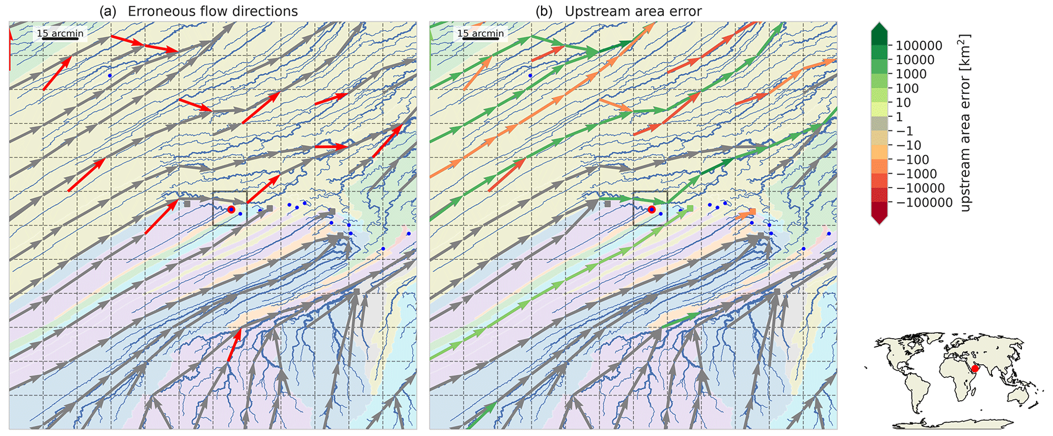
Figure C1 Largest endorheic basin (6996 km²) which is not resolved at the 15 arcmin resolution indicated with a highlighted basin pit. The blue lines show the fine-resolution river; the background colors show basin boundaries; the dashed lines show the coarse-resolution grid, and the arrows show the upscaled flow directions pointing from the outlet pixel or the original cell to the outlet pixel of the destination cell. Flow directions are red if erroneous (a), and green denotes a positive and red a negative upstream area error (b).

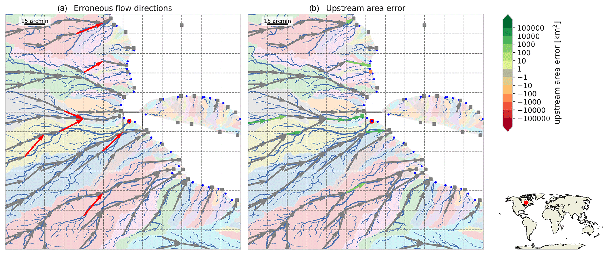
Figure C2 Largest exorheic basin (6830 km²) which is not resolved at the 15 arcmin resolution indicated with a highlighted basin outlet. See the caption of Fig. C1 for a full description.

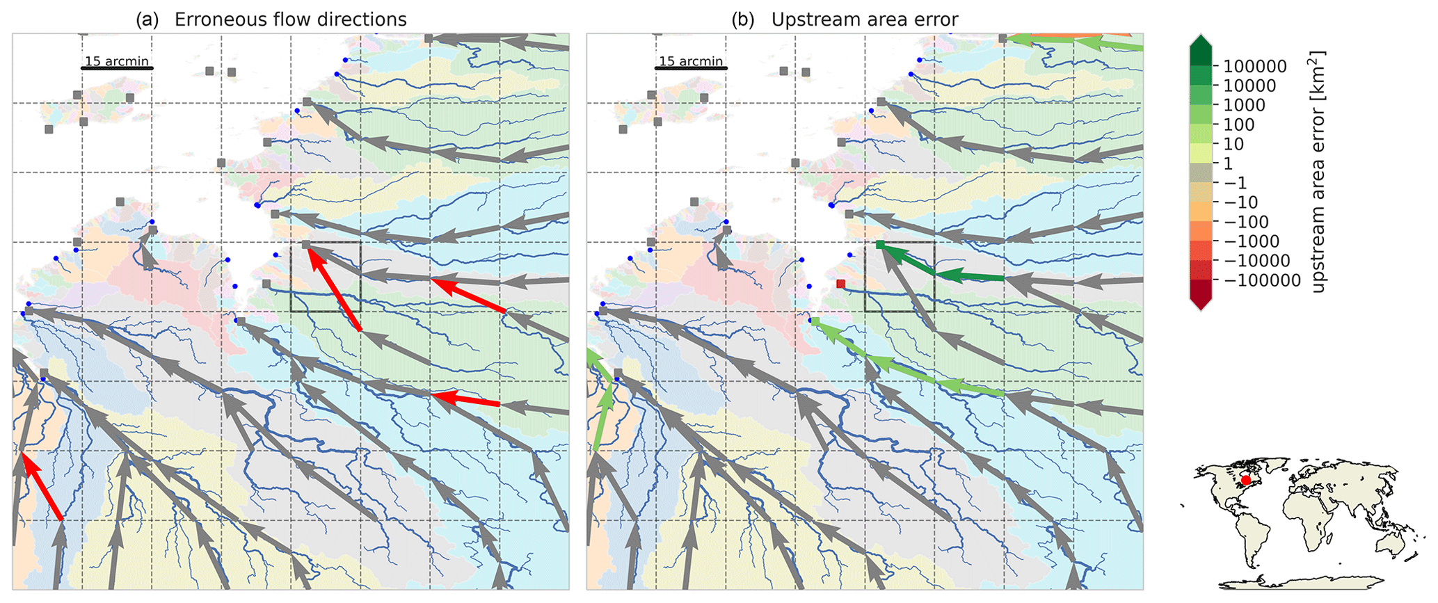
Figure C3 Largest basin (914 km²) with a relative upstream area error of more than 10 % at the 30 arcsec resolution indicated with a highlighted cell. See the caption of Fig. C1 for a full description.

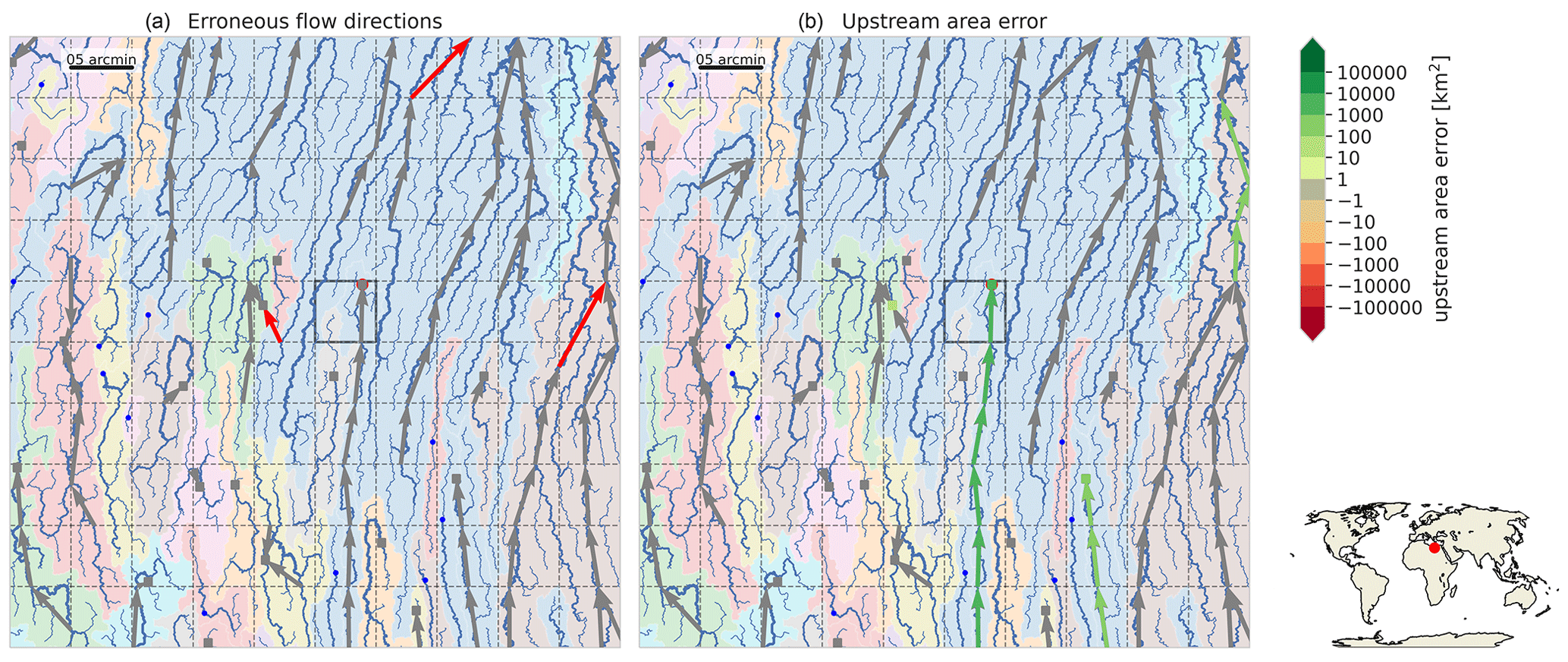
Figure C4 Largest basin (16 717 km²) with a relative upstream area error of more than 10 % at the 5 arcmin resolution indicated with a highlighted cell. See the caption of Fig. C1 for a full description.

Figure C5 Largest basin (42 017 km²) with a relative upstream area error of more than 10 % at the 15 arcmin resolution indicated with a highlighted cell. See the caption of Fig. C1 for a full description.

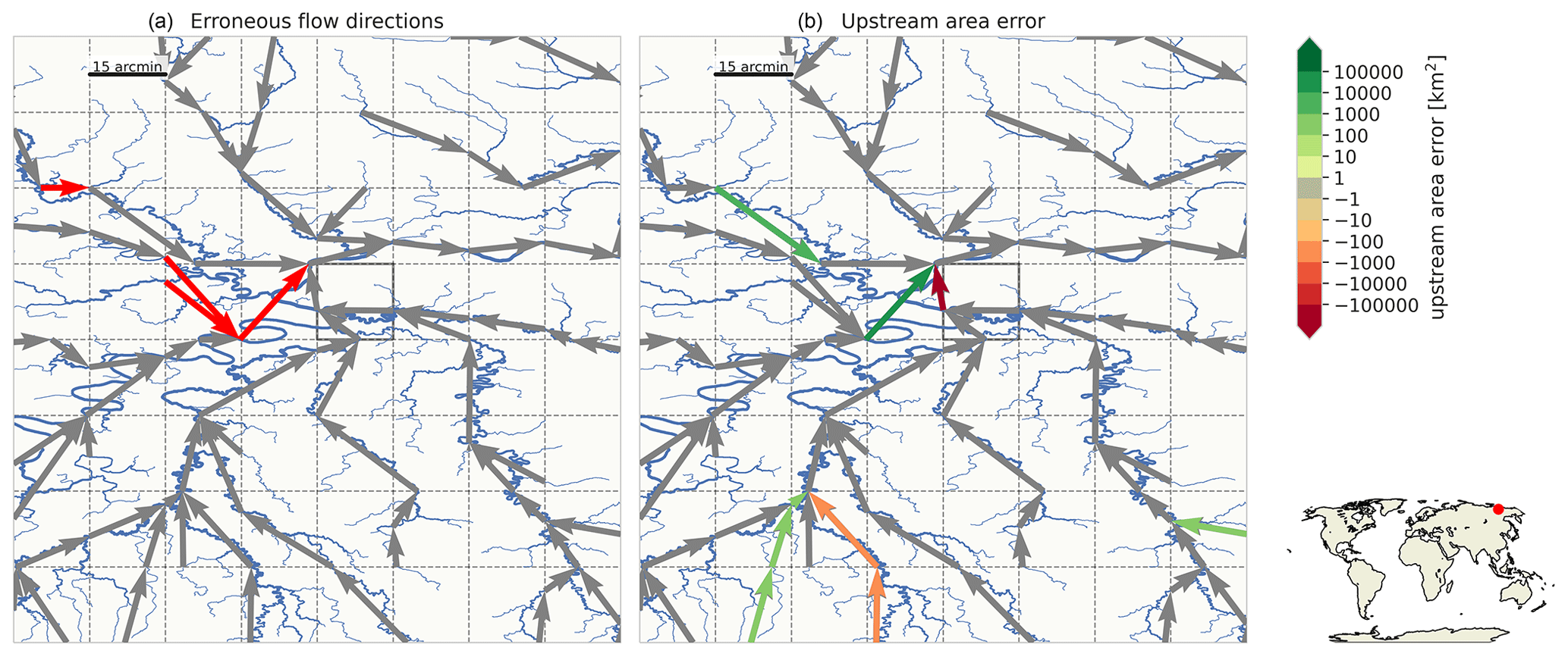
Figure C6 Second-largest local upstream area error (−220 876 km²) at the 15 arcmin resolution indicated with a highlighted cell. See the caption of Fig. C1 for a full description.

Appendix D: Accuracy benchmark of upscaling methods

This section shows maps of the relative upstream area error at resolutions of 30 arcsec and 15 arcmin in addition to the map at 5 arcmin as presented in Sect. 3.

Figure D1 Percentage of cells at a 30 arcsec (∼ 1 km) resolution per 1×1^∘ tile with an absolute relative upstream area error of more than 1 %. The markers show the upstream area error at the basin outlet and the black lines the outlines of the 200 largest basins globally.

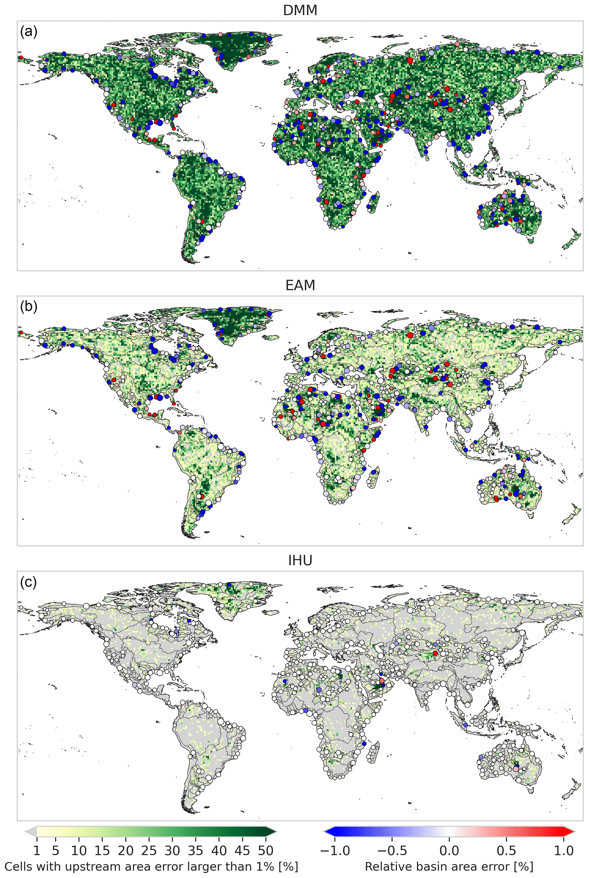
Figure D2 Percentage of cells at a 15 arcmin (∼ 30 km) resolution per 1×1^∘ tile with an absolute relative upstream area error of more than 1 %. The markers show the upstream area error at the basin outlet and the black lines the outlines of the 200 largest basins globally.

Appendix E: Sensitivity analysis – IHU parameters

The sensitivity of the R parameter to define the effective area in step 1-1 (see Eq. 1) as well as the minimum length and minimum upstream area thresholds used to optimize sub-grid river length in step 3, see Sect. 2.1, is tested for the Rhine basin.

We tested the sensitivity to these thresholds based on four metrics expressed as a percentage of the basin cells at various resolutions. Two upscaling accuracy metrics – flow direction error and relative upstream area >1 % as explained in Sect. 3.2 – as well as a metric to assess the number of cells with a small sub-grid cell area (i.e., < 25 % of cell area) and small sub-grid river length (i.e., < 25 % of cell length) are used.

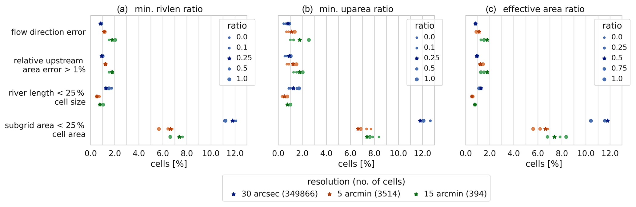
Figure E1 Sensitivity analysis for the minimum river length threshold (a), minimum upstream area threshold (c) and effective area definition (c), where the minimum river length threshold and R parameter in the effective area definition are expressed as a ratio of the cell size and the minimum upstream area threshold as a ratio of the cell area. The sensitivity is tested for four metrics (y axis) and expressed as a percentage of the total basin cells (x axis). The default ratio is shown with a star and alternative ratios with dots for which the size is scaled with the ratio value.

Appendix F: Sensitivity analysis – runoff experiment

The sensitivity of the model similarity between upscaled and baseline resolution models to three key model variables is presented in this section. The similarity is expressed as the difference in flood peak timing and magnitude between the upscaled and native-resolution model.

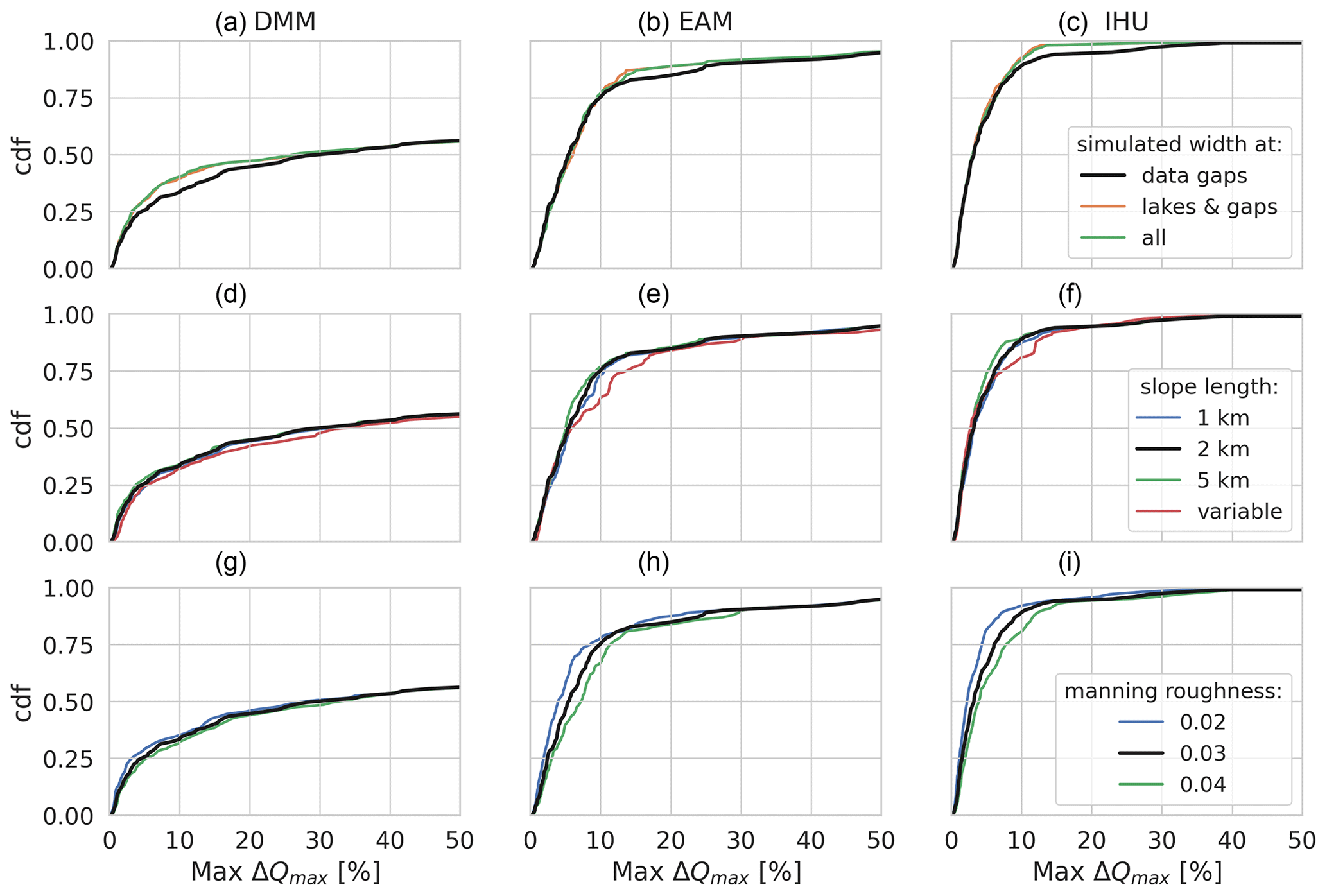
Figure F1 Sensitivity analysis of the relative difference in simulated peak magnitude for a case study in the Rhine basin for three parameters (rows) and for three upscaling methods (columns). Each plot shows the CDF of all output locations on the y axis and the relative difference in simulated peak magnitude on the x axis. The first row shows the sensitivity to the average MERIT Hydro vs. power-law-based channel width estimates; the second row shows the sensitivity to the minimum channel length over which the channel slope is estimated, and the third row shows the sensitivity to the Manning roughness coefficient. The black line is the default case in all plots.

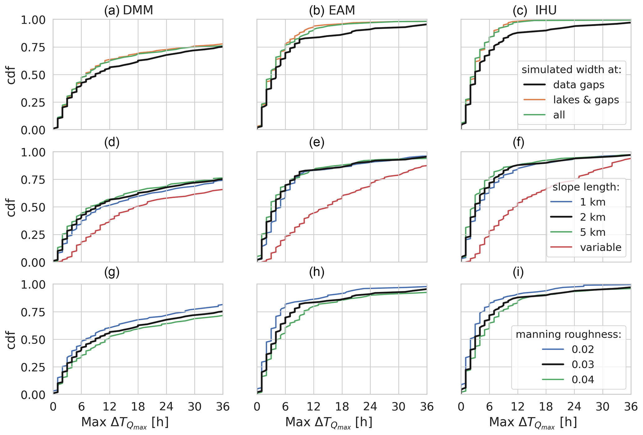
Figure F2 Sensitivity analysis of the relative difference in simulated peak timing for a case study in the Rhine basin for three parameters (rows) and for three upscaling methods (columns). Each plot shows the CDF of all output locations on the y axis and the relative difference in simulated peak magnitude on the x axis. The first row shows the sensitivity to the average MERIT Hydro vs. power-law-based channel width estimates; the second row shows the sensitivity to the minimum channel length over which the channel slope is estimated, and the third row shows the sensitivity to the Manning roughness coefficient. The black line is the default case in all plots.