A 10 km North American precipitation and land-surface reanalysis based on the GEM atmospheric model

Environment and Climate Change Canada has initiated the production of a 1980–2018, 10 km, North American precipitation and surface reanalysis. ERA-Interim is used to initialize the Global Deterministic Reforecast System (GDRS) at a 39 km resolution. Its output is then dynamically downscaled to 10 km by the Regional Deterministic Reforecast System (RDRS). Coupled with the RDRS, the Canadian Land Data Assimilation System (CaLDAS) and Precipitation Analysis (CaPA) are used to produce surface and precipitation analyses. All systems used are close to operational model versions and configurations. In this study, a 7-year sample of the reanalysis (2011–2017) is evaluated. Verification results show that the skill of the RDRS is stable over time and equivalent to that of the current operational system. The impact of the coupling between RDRS and CaLDAS is explored using an early version of the reanalysis system which was run at 15 km resolution for the period 2010–2014, with and without the use of CaLDAS. Significant improvements are observed with CaLDAS in the lower troposphere and surface layer, especially for the 850 hPa dew point and absolute temperatures in summer. Precipitation is further improved through an offline precipitation analysis which allows the assimilation of additional observations of 24 h precipitation totals. The final dataset should be of particular interest for hydrological applications focusing on transboundary and northern watersheds, where existing products often show discontinuities at the border and assimilate very few – if any – precipitation observations.

1 Introduction

Atmospheric reanalysis datasets are invaluable tools allowing for better understanding and analysis of global and regional water cycles by integrating data assimilation techniques with state-of-the-art numerical models of the atmosphere and Earth's surface observations of the water and energy cycle. Indeed, this was one of the main objectives in the design and the development of recent reanalysis datasets such as National Aeronautics and Space Administration (NASA) Modern-Era Retrospective analysis for Research and Applications (MERRA) (Bosilovich et al., 2008, 2011; Rienecker et al., 2011; Takacs et al., 2016), European Centre for Medium-Range Weather Forecasts (ECMWF) interim reanalysis (ERA-Interim) (Dee et al., 2011) and ECMWF reanalysis fifth generation (ERA5) (Hersbach et al., 2020).

Data assimilation is the process by which a system state estimated by a model is merged with observations of that system, in order to adjust the trajectory of the model (Fletcher, 2017). More specifically, a gridded numerical model output (commonly referred to as the background or trial field) is combined with observations of all kinds, through advanced mathematical methods constrained by the laws of physics in order to obtain a gridded representation (generally referred to as an analysis) as close as possible to the true state which the numerical model intends to predict and observations intend to measure.

Atmospheric reanalysis datasets are generally obtained by performing data assimilation of atmospheric observations every few hours and integrating a numerical weather prediction (NWP) model between analysis times. The NWP model itself relies on a land-surface scheme to represent energy, mass and momentum exchanges occurring at the Earth's surface. Most reanalyses are designed to provide optimal results for large-scale atmospheric fields, sometimes at the price of degradation of surface prediction skill and bias (Albergel et al., 2013; Fujiwara et al., 2017). In addition, reanalyses often do not assimilate any observations of precipitation and of the land-surface state but instead only provide short-term forecasts of these variables.

Another limitation of existing atmospheric reanalyses is that their spatial resolution can be too coarse to be fully suited for land-surface applications at the regional scale (Marke et al., 2011), even for the most recent and advanced ones such as ERA5 (Hersbach et al., 2020) or the North American Regional Reanalysis (NARR; Mesinger et al., 2006), which have a resolution of approximately 30 km. In order to obtain predictions at the scale required for many land-surface and hydrological modelling applications, higher-resolution atmospheric forcing and land-surface model outputs are necessary. For example, in regions of France showing high precipitation variability, Lobligeois et al. (2014) note a significant improvement in streamflow simulations when gridded rainfall is provided to a hydrological model at a resolution of 8 km or better. In studies conducted in China, Shrestha et al. (2002, 2006) report better hydrological simulation results when the number of grid cells per watershed is at least 10, meaning that 30 km resolution would only be appropriate for watersheds of size 1000 km² or larger. Nevertheless, Tarek et al. (2020) report satisfactory results over North America when using ERA5 precipitation and temperature to drive a lumped hydrological model, even for watersheds of less than 1000 km² in size (although the skill does increase with watershed size).

As a consequence, separate and complementary land-surface reanalyses have been developed by both NASA and ECMWF where the above-mentioned atmospheric reanalyses are directly used to force advanced land-surface models in an open-loop manner and at higher horizontal resolution. Considering that precipitation is one of the most influential forcings for land-surface processes, precipitation is generally adjusted and locally rescaled based on observation datasets such as the Global Precipitation Climatology Project pentad – GPCP v2.1 (Adler et al., 2003). Such datasets, including MERRA-Land (Reichle et al., 2011), ERA-Interim-Land (Balsamo et al., 2015) and ERA5-Land (Muñoz Sabater et al., 2018) are shown to improve surface prediction when compared to the underlying original reanalysis. However, with the exception of a simple precipitation adjustment, data assimilation of neither surface nor remotely sensed observations is involved in the process. Going one step further, optimal interpolation was used by Soci et al. (2016) to create reanalyses of temperature, humidity and precipitation over Europe at high spatial resolution (5.5 km) and over a short historical period (2007–2010) by combining short-term forecasts of an operational NWP model with in situ observations using the MESCAN analysis system. This approach is interesting but difficult to apply over a long historical period, since the outputs from the same NWP model would not be available.

The main objectives of this paper are (1) to present a strategy for the production, at relatively low computing cost, of high-resolution surface and precipitation regional reanalyses which includes two-way coupling between the land data assimilation system and the NWP model, as well as assimilation of precipitation observations, and (2) to evaluate a North American reanalysis based on the Global Environmental Multiscale (GEM) model (Côté et al., 1998a, b; Girard et al., 2014), obtained using the proposed methodology and currently under production at the Canadian Centre for Meteorological and Environmental Prediction (CCMEP) of Environment and Climate Change Canada (ECCC).

The desired outputs from this system are hourly time series, available on a ∼10 km regular grid of the main meteorological variables that are required in order to operate surface and hydrology models: near-surface air temperature, near-surface air humidity, surface pressure, wind speed and direction, incoming infrared flux at the surface, downward solar flux at the surface, and finally precipitation.

One of the important motivations for the production of this reanalysis is, for ECCC, to better support the International Joint Commission (IJC), which prevents and resolves disputes related to transboundary watersheds covered by the Canada–US Boundary Waters Treaty. Too often, North American climate datasets show discontinuities at the Canada–US border (Gronewold et al., 2017). By covering seamlessly all of North America, this product is expected to facilitate hydrometeorological and hydroclimatic studies involving transboundary watersheds in North America.

1.1 Open-loop land-surface simulations as an alternative to reanalysis land-surface data

The approach used by ERA5-Land, MERRA-Land and ERA-Interim-Land of running a land-surface model in open loop with adapted meteorological forcing data is fairly common in the land-surface and hydrology modelling community (Albergel et al., 2013; Muñoz Sabater et al., 2018), i.e. surface models are often integrated in an open-loop manner forced by some kind of atmospheric gridded datasets in order to predict the state of the land surface. There are several major advantages to this approach: (1) atmospheric forcing can be improved through postprocessing, (2) horizontal resolution can be increased without a prohibitive computational cost, and (3) a more recent land-surface scheme, or perhaps more adapted to the problem at hand, can be used. While convenient and relatively straightforward, results from this approach are fully dependent on both the forcing data quality and the abilities of the land-surface model when used with this specific forcing dataset to reproduce the processes of interest. No observations are directly involved other than those used to produce the atmospheric forcing. Thus the land-surface model errors can grow over time since the land-surface model is allowed to drift without the constraints from surface observations. These errors can be caused by limitations of the land-surface scheme but also by an imbalance between the atmospheric forcing obtained from a reanalysis product and the surface feedback predicted by the land-surface model when a different horizontal resolution or different model is used.

1.2 Dynamical downscaling of reanalysis data to improve horizontal resolution

The resolution limitation of existing reanalysis products can be overcome through dynamical downscaling, using either a limited-area NWP model or a regional climate model. This is once again fairly common in the literature; see for example Yoshimura and Kanamitsu (2008) and Giorgi (2019). Such models, when initialized and/or forced at their boundaries with reanalysis data have been shown to perform properly and can improve results (Lucas-Picher et al., 2013; Chikhar and Gauthier, 2014). When the objective is to generate high-resolution datasets covering periods of more than a few years, this approach is generally preferable to the use of archived outputs from operational analysis and/or forecasting systems. Indeed, although operational analyses and forecasts can be more skilful than reanalyses, these datasets are not consistent in time; i.e. their time and space resolution and quality evolve as a function of operational implementations, preventing their usage for long-term applications where consistency is required (Smith et al., 2014).

The atmospheric model used for dynamical downscaling generally relies on a land-surface model sufficiently different from the one used as part of the lower-resolution reanalysis system. As a result, it cannot be initialized from land-surface state variables provided with the reanalysis. The usual solution to this problem is to continuously integrate the land-surface model, cycling the land-surface state variables after the end of each atmospheric model run. Again, the land-surface model is allowed to drift with time. Furthermore, because the land-surface model interacts with the atmospheric model in a dynamical downscaling experiment, the atmospheric model itself can drift with time. It will be shown that this feature of the standard approach to dynamical downscaling of reanalyses can lead to significant atmospheric model errors and biases.

1.3 Avoiding land-surface and atmospheric model drift through land-surface data assimilation

Land-surface model drift can be controlled through the use of a land-surface data assimilation system (Carrera et al., 2015). At the same time, the surface analyses provided by such a system can be used to better initialize an atmospheric model used for dynamical downscaling if the same land-surface model is used by the land-surface data assimilation system and the atmospheric prediction system. The dynamically downscaled atmospheric forcing can furthermore be used as input to the land-surface data assimilation scheme, thus ensuring consistency between the surface predictions performed as part of the assimilation and forecast cycles. The computing cost of such an approach is higher than that of running an open-loop simulation, but still much less than that of a complete atmospheric and land-surface reanalysis (Fairbairn et al., 2017). It will be shown that coupling a land-surface data assimilation scheme with a limited area NWP model for dynamical downscaling is well worth the effort as it leads to significantly improved near-surface atmospheric and land-surface predictions.

1.4 Structure of the paper

The present study documents a methodology for increasing the resolution of a reanalysis product through dynamical downscaling while avoiding model drift near the surface through land-surface data assimilation. Two versions of this reanalysis are introduced and evaluated: a preliminary version with a horizontal resolution of 15 km is used to assess the impact of the land-data assimilation system over the period 2010–2014, and a second version with a horizontal resolution of 10 km is compared over the period 2010–2017 to the operational NWP system which was in operation at CCMEP over the same time period. This atmospheric reforecast and land-surface reanalysis covers the whole North America and the Arctic Ocean, and the evaluation is performed over Mexico, the United States of America and Canada. In Sect. 2, the methodology followed to obtain such a product is presented, along with the observational datasets involved in land-surface and precipitation data assimilation. Verification metrics used throughout the paper are also introduced. In Sect. 3, the added value of surface data and precipitation assimilation versus more standard dynamical downscaling approaches is assessed both from a surface perspective and with regards to the free atmosphere, based on the 15 km configuration of the reanalysis. Section 4 focuses on the evaluation of precipitation, temperature dew point from the 15 and 10 km configurations, relying on surface and streamflow observations. A discussion and conclusion follow.

2 Data and method

When designing a reanalysis system, many decisions have a significant impact on the resources and time required to perform the reanalysis. Despite these constraints, horizontal resolution must be sufficient to allow for an acceptable representation of the hydrological cycle. Benedict et al. (2019) suggest that 25 km is likely insufficient to represent the climatic driver of the Mississippi river basin, but Deacu et al. (2012) obtained satisfactory results when simulating the net basin supplies of the Great Lakes basin at 15 km resolution.

Based on the results of Deacu et al. (2012), initial tests aimed at fine-tuning the configuration of the reanalysis system were performed at 15 km resolution. However, a resolution of 10 km was chosen for the production of a 1980–2018 reanalysis, in order to match the current resolution of the Regional Deterministic Prediction System (RDPS) and of the Regional Ensemble Prediction System (REPS) currently in operation at CCMEP for short-term weather forecasting over North America.

Having settled on a system operating at the meso-gamma scale over North America, the system was designed in order to provide all atmospheric forcing required to perform land-surface and hydrological modelling at the regional scale and to be coherent with in situ surface observations (e.g. precipitation, absolute and dew point temperatures, and snow depth) while avoiding the need for atmospheric data assimilation.

As illustrated in the left panel of Fig. 1, the global reanalysis ERA-Interim (Dee et al., 2011) is used as initial atmospheric conditions of the so-called Global Deterministic Reforecast System (GDRS) in order to produce a global reforecast at higher resolution than ERA-Interim. Then, following a dynamical downscaling approach, the so-called Regional Deterministic Reforecast System (RDRS) is applied, also initialized by ERA-Interim (Dee et al., 2011) but driven by the GDRS, to produce a reforecast at higher resolution covering the whole North America and Arctic Ocean. Both the GDRS and RDRS are based on the GEM model (respectively on global and regional configurations of GEM).

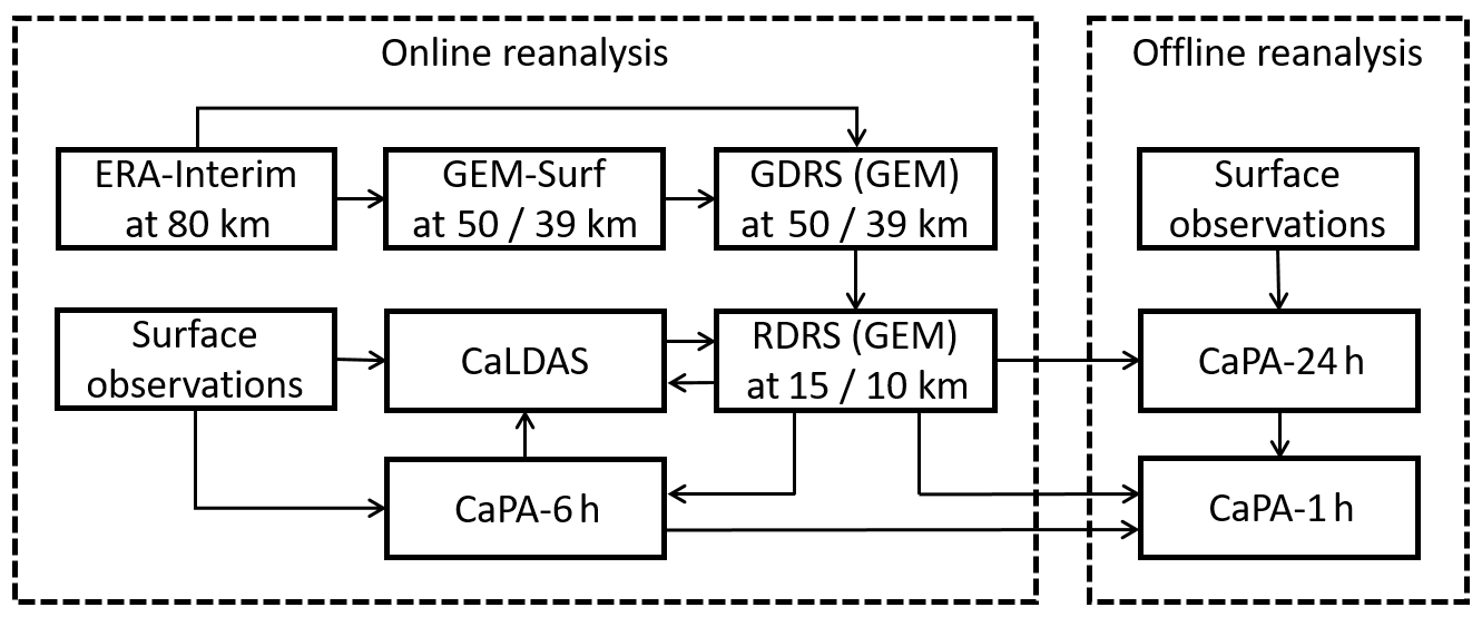
Figure 1 Scheme illustrating the main components of the method followed to produce a land-surface and precipitation reanalysis.

ERA-Interim, and not ERA5, is used for initializing the GDRS and RDRS mainly because ERA5 was not available during the development phase of this reanalysis project.

Surface initial conditions (sea surface temperature, sea ice concentration and thickness, soil moisture, soil temperature, and snowpack conditions) consistent with the driving data and the surface scheme of the atmospheric model are also required. For the GDRS, initial land-surface conditions are obtained from an a priori offline (open-loop) of GEM's land-surface model, GEM-Surf (Carrera et al., 2010; Bernier and Bélair, 2012), directly forced by the near-surface fields of the ERA-Interim reanalysis as well as the 3 h precipitation amounts (Gagnon et al., 2015). This offline system relies on a version of the Interaction Soil–Biosphere–Atmosphere (ISBA) land-surface scheme (Noilhan and Planton, 1989; Noilhan and Mahfouf, 1996) adapted for use in the GEM model (Bélair et al., 2003a, b), as well as sea ice and glacier schemes which are part of the GEM model itself.

To improve initial conditions of soil moisture, soil temperature and snow depth, the RDRS is coupled with the Canadian Precipitation Analysis (CaPA) (Mahfouf et al., 2007; Lespinas et al., 2015; Fortin et al., 2015, 2018) and the Canadian Land Data Assimilation System (CaLDAS) (Brasnett, 1999; Balsamo et al., 2007; Carrera et al., 2015) as detailed hereafter.

In this section, the main aspects of the global and regional atmospheric reforecasts, as well as the precipitation and surface data assimilation systems, are presented. Then, observational datasets used for data assimilation as well as verification metrics used throughout the paper are introduced.

In order to reduce the risk of discovering major issues with the reanalysis after the fact, GDRS, RDRS, CaPA and CaLDAS configurations are kept as close as possible to documented configurations and currently operational versions of these systems at CCMEP. More details on the configuration of each component are given below.

2.1 Atmospheric model

Both GDRS and RDRS were based on the latest stable version of the Global Environment Multiscale (GEM v4.8-LTS) model (Côté et al., 1998b, a; Girard et al., 2014) at the time of production. Their configurations, as summarized in Tables 1 and 2, are closely related to the control member of the Global and Regional Ensemble Prediction System (GEPS and REPS) (Li et al., 2008; Lavaysse et al., 2012; Houtekamer et al., 2013; Gagnon et al., 2015; Lin et al., 2016) as well as the Regional Deterministic Prediction System (RDPS) (Bélair et al., 2005; Mailhot et al., 2006; Caron et al., 2016).

(Girard et al., 2013)(Côté et al., 1998b, a)(Fillion et al., 1995)(Li and Barker, 2005)(Bélair et al., 2003a, b)(Kain and Fritsh, 1990; Kain and Fritsch, 1993)Mailhot et al., 1998(see Bélair et al., 2005)Sundqvist et al. (1989)(see Pudykiewicz et al., 1992)Bélair et al. (2009)McFarlane (1987); McFarlane et al. (1986)Hines (1997a, b)(Lott and Miller, 1997; Zadra et al., 2003)Benoit et al. (1989)Bélair et al. (1999)Bélair et al. (2005)(McTaggart-Cowan and Zadra, 2014)

Table 1 Dynamic kernel and physical parameterizations common to the GDRS and RDRS.

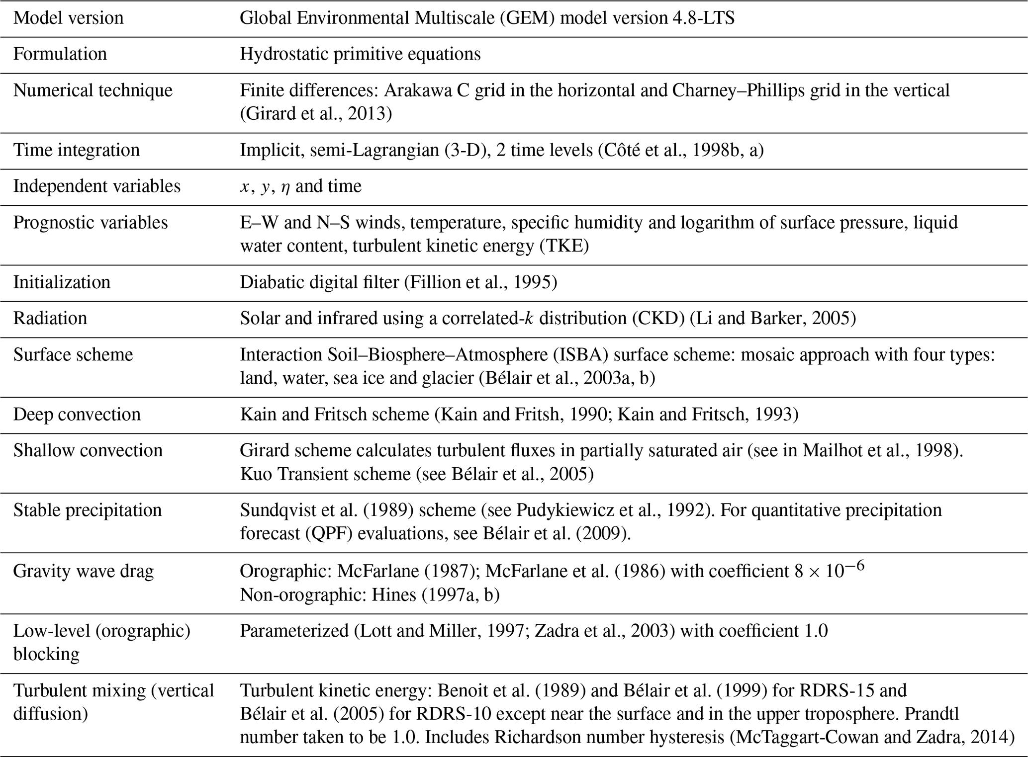
Table 2 Main differences in the configuration of the GDRS and RDRS.

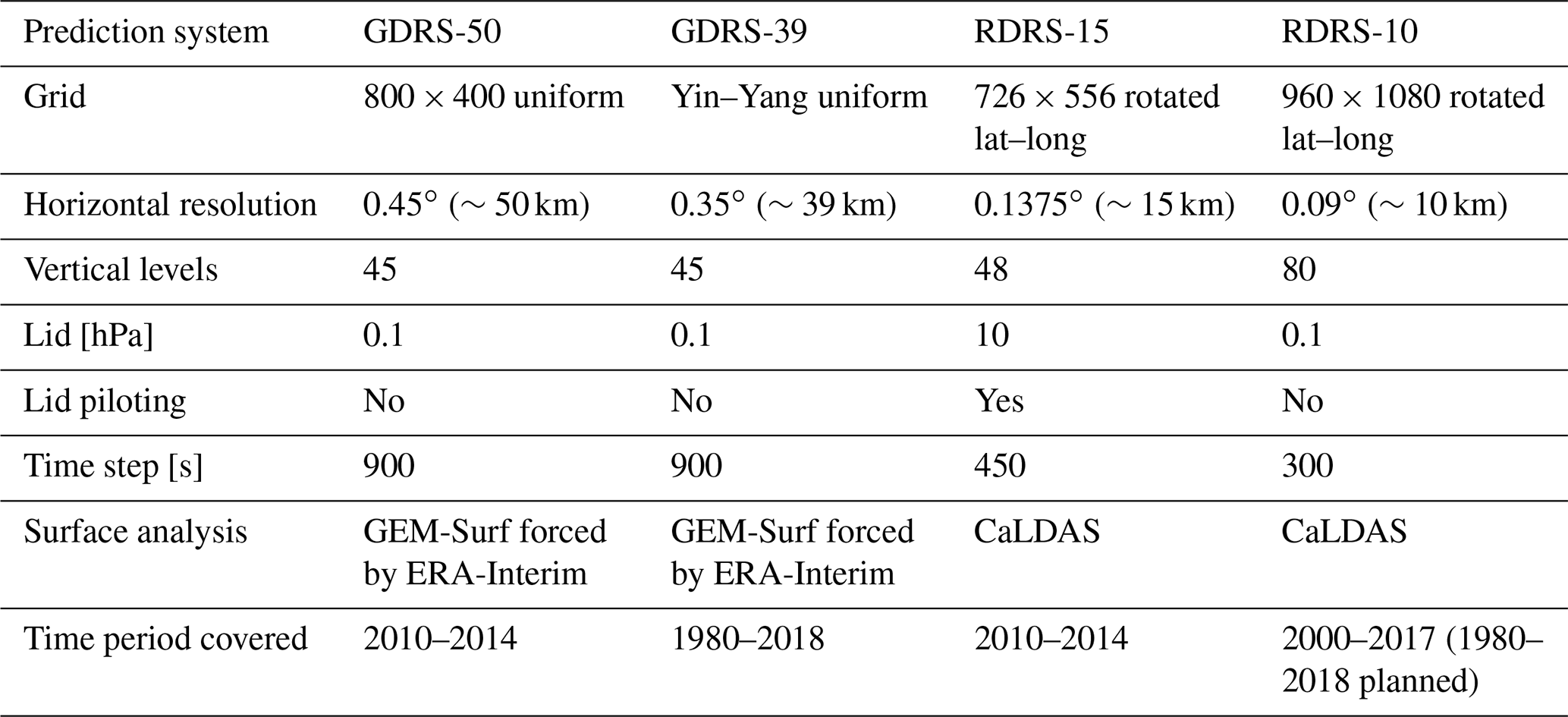
Two configurations of the RDRS were used in this study: RDRS-15, having a horizontal resolution of 15 km (which is based on REPS control member configuration), and RDRS-10, having a horizontal resolution of 10 km (which is based on RDPS configuration). RDRS-15 was nested in a configuration of the GDRS, having a resolution of 50 km (GDRS-50), and RDRS-10 in a configuration of the GDRS, having a resolution of 39 km (GDRS-39). As will be explained later, the GDRS and RDRS are initialized at both 00:00 and 12:00 UTC. The following nomenclature will be used to refer to a specific model configuration and initial time: AAAAZZ-HH, where AAAA refers to the prediction system (either GDRS or RDRS), ZZ to the initial time (either 00:00 or 12:00 UTC) and HH to the horizontal resolution. For example, RDRS00-10 refers to the 00:00 UTC run of the 10 km configuration of the RDRS. ZZ and/or -HH will be omitted when obvious from the context or when the statement or conclusion applies independently of either the initial time or the horizontal resolution.

The GDRS-50 features a global uniform latitude–longitude grid with 800×400 meshes of 0.45^∘, while the GDRS-39 features a Yin–Yang grid (Qaddouri and Lee, 2011), having a uniform resolution of 0.35^∘ (having a total of $\mathrm{2}\times \mathrm{835}\times \mathrm{303}$ meshes). The GDRS features 45 staggered hybrid vertical levels going from the surface up to 0.1 hPa (lid of the model). A 900 s time step is used. RDRS-15 (resp. RDRS-10) features a limited area rotated uniform latitude–longitude grid with 726×556 (resp. 960×1080) meshes. The grid covers North America, adjacent oceans, the whole Arctic Ocean and part of Europe and Siberia. A 450 s (resp. 300 s) time step is used. In the vertical, it features 48 (resp. 80) hybrid staggered vertical levels going from the surface up to 10 (resp. 0.1) hPa. In all configurations of GDRS and RDRS, the first momentum level is at ∼40 m and the first thermodynamic level is at ∼20 m.

While similar, configurations of GDRS and RDRS are adapted to their grid configuration: (a) a few parameters differ as required by the resolution change, (b) additional diffusion is added at the pole of GDRS-50, (c) in RDRS-15, an upper-boundary nesting procedure is used (McTaggart-Cowan et al., 2011) in addition to the usual lateral boundary nesting, and (d) in RDRS-10, a more advanced turbulent kinetic energy (TKE) closure is used to take into account boundary layer clouds (Bélair et al., 2005).

Concerning input geophysical fields (i.e. orography, surface roughness length (except over water), subgrid-scale orographic parameters for gravity wave drag and low-level blocking, vegetation characteristics, soil thermal and hydraulic coefficients, and glaciers fraction), the same input databases and processing methods are used in the GDRS and RDRS as in the operational systems, albeit to produce fields at a different resolution. They are derived from a variety of recent geophysical databases using an in-house software (GenPhysX v2.3.4; Zadra et al., 2008) and are fixed in time.

Finally, both the GDRS and the RDRS are launched twice a day (every 12 h at 00:00 and 12:00 UTC) and integrated for 24 h in an intermittent cycling manner. Both rely on the 37 pressure levels from ERA-Interim as initial atmospheric conditions of the five main variables of GEM. To avoid the effect of initial shock, a diabatic filtering procedure (Fillion et al., 1995) is applied at the beginning of each integration, i.e. during the first 6 h in the GDRS and the first 3 h in the RDRS. Thus, given the resolution jump, with the spin-up required for some of the variables such as cloud and precipitation and this filtering procedure, it was decided to avoid using the data for the first 6 h following the beginning of the integration for land-data assimilation purposes.

Outputs from GDRS-50 and RDRS-15 are available for a 5-year test period (2010–2014), whereas outputs from GDRS-39 are available for most of the period covered by ERA-Interim (1980–2018). Outputs from RDRS-10 will be produced for the same period by CCMEP and are already available for 2000–2017 (1980–2018 planned).

2.2 Surface assimilation

The land-surface treatment (soil moisture, soil temperature and snowpack conditions) differs notably between the GDRS and RDRS. For the GDRS, as shown in Figs. 1 and 2, initial conditions of each simulation are obtained from an a priori offline simulation of the CCMEP land-surface model, GEM-Surf (Carrera et al., 2010; Bernier and Bélair, 2012), directly forced by ERA-Interim atmospheric variables.

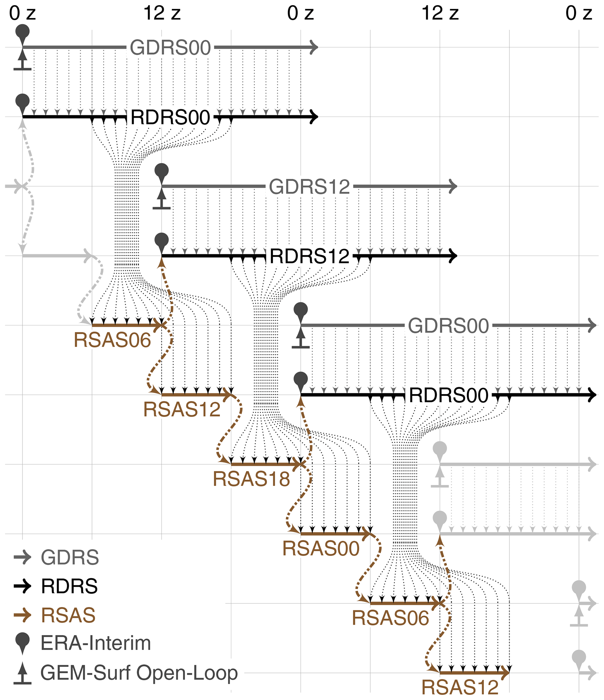
Figure 2 Flowchart of the method followed to produce a land-surface and precipitation reanalysis.

For its part, the RDRS is coupled with CaLDAS (Balsamo et al., 2007; Carrera et al., 2015), meaning that the latter is driven by the RDRS which then uses the surface analyses produced by CaLDAS as surface initial conditions for the next integration as illustrated in Fig. 2. CaLDAS uses a one-dimensional ensemble Kalman filter (EnKF) to estimate soil moisture and soil temperature and an optimal interpolation (OI) scheme to estimate snow depth. In addition, considering that precipitation is one of the main drivers of surface and soil processes, CaLDAS further relies on the Canadian Precipitation Analysis (CaPA) (Mahfouf et al., 2007; Lespinas et al., 2015; Fortin et al., 2018) system to provide it with a 6 h precipitation analysis as input. CaPA relies on an OI method similar to the one used for snow depth. In all cases, an ensemble of analyses is obtained by perturbing the meteorological inputs to the land-surface scheme, as described by Carrera et al. (2015). The combination of CaPA and CaLDAS configurations designed to initialize the GEM model in its regional configuration is known as the Regional Surface Analysis System (RSAS). All the analyses are performed at the resolution of the background field for a subdomain covering the whole North America (co-located meshes with RDRS). Furthermore, in order to avoid using data within the spin-up period of the model, only data from the 6 to 18 h reforecast lead time serves as background as shown in Fig. 2.

Figures 1 and 2 sum up this approach. Each RSAS analysis cycle runs for 6 h, because precipitation and snow depth analyses are only available every 6 h (analyses for all others land-surface variables are available every 3 h). Hence, following such an approach allows for combining surface observations of temperature, humidity, snow depth and precipitation with the first guess provided by the RDRS and GEM-Surf through various OIs and a one-dimensional EnKF (Brasnett, 1999; Balsamo et al., 2007; Carrera et al., 2015; Fortin et al., 2015).

2.3 Precipitation analysis

As already mentioned, CaPA (Mahfouf et al., 2007; Lespinas et al., 2015) is the system used to produce gridded precipitation analysis for 6 and 24 h accumulation periods. CaPA combines precipitation observations with a background field obtained from the short-term reforecast provided by the RDRS through an OI method. It aims to correct the error of the latter by spatially interpolating in a transformed space (cubic-root transformation) the differences between the observed values and the corresponding background values at the station locations. Error statistics (standard deviations of background errors and of observation errors and the characteristic length scale) required to perform the OI are continuously updated based on a temporally adaptive method, allowing us to implicitly consider seasonal changes in precipitation characteristics (and evolving model error). CaPA also includes an advanced quality control of observations (Lespinas et al., 2015). Although the operational configuration of CaPA assimilates radar quantitative precipitation estimates (Fortin et al., 2015), no radar data are used in this study, due to the availability and the complexity of accessing, processing and controlling the quality of radar data for such a long period in the past.

CaPA has been applied successfully in a number of studies, oftentimes demonstrating great capabilities. See Fortin et al. (2018) for a recent literature review. It is currently operational at CCMEP, providing near real-time precipitation analysis over North America at 10 km resolution and over most of Canada at 2.5 km resolution.

Given that precipitation is one of the most influential forcing of land-surface processes, CaPA serves to provide CaLDAS with 6 h precipitation analysis as illustrated in Fig. 1. For that sake, 1, 3 and 6 h precipitation accumulation observations from the different networks covering the whole North America are assimilated. In order to represent the uncertainty in both the background field and the observations, an ensemble of CaPA 6 h analyses are actually generated in the process (see Carrera et al., 2015, for more details). This precipitation analysis will be later referred to as CaPA-6h.

Several precipitation observation networks, notably the ones that are subject to the most advanced offline quality control and adjustments (see Sect. 2.5), are, however, only available for daily accumulations. As a result, these networks cannot be used directly in the production of the reanalysis as previously described. Hence, in order to take advantage of such networks, CaPA is run again but for 24 h precipitation accumulations in an a posteriori manner based on the first guess provided by RDRS. More precisely, in order to prevent users from using data in the spin-up period of the model, the 6 to 18 h forecast lead time from various sequential integrations are used to build 24 h accumulations valid at 12:00 UTC as illustrated in Fig. 3. The latter then serve as a background field in order for CaPA to produce 24 h precipitation analyses covering the whole domain and period of interest, later referred to as CaPA-24h.

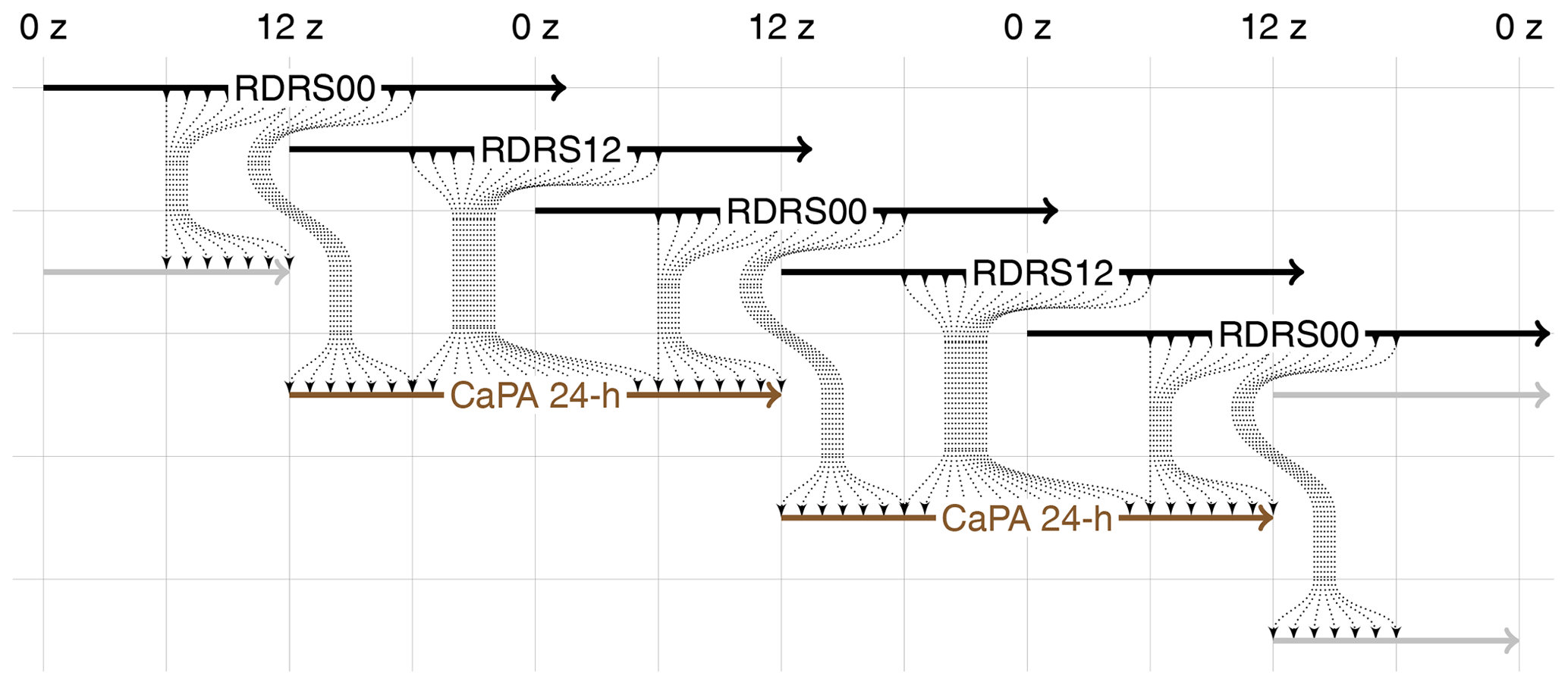
Figure 3 Flowchart illustrating the approach to build 24 h accumulation and produce 24 h precipitation analysis at 12:00 UTC based on 6 to 18 h lead time RDRS outputs from integrations started at 00:00 and 12:00 UTC.

Strict quality control procedures are in place in both CaPA-6h and CaPA-24h to avoid the assimilation of biased observations, and in particular wind-induced undercatch of solid precipitation. If, based on a temperature analysis, solid precipitation is likely to have fallen in the gauge, wind speed observations are used to determine if a precipitation observation should be assimilated. Different wind speed thresholds are used depending on the network, the type of gauge and whether the station is manned or automated (see Lespinas et al., 2015, for more details on the quality control procedure).

An important difference between CaPA-6h and CaPA-24h is that the former is part of CaLDAS and thus contributes to the initialization of the atmospheric model, whereas the latter serves to improve the final precipitation product through a postprocessing step that can be launched a posteriori once all integrations of the atmospheric model have been performed. Hence, it is possible to reprocess the final 24 h precipitation product at a small computational cost if more precipitation datasets (or datasets of better quality) become available.

For many environmental modelling applications, a 24 h time step for a precipitation product is too coarse. In order to provide users with realistic hourly precipitation rates and accurate accumulations, the CaPA-24h precipitation analysis has been disaggregated to an hourly time step using a two-step procedure. Firstly, the CaPA-6h is disaggregated to an hourly time step by linearly rescaling the atmospheric model's hourly precipitation rates in order to match the 6 h accumulations estimated by CaPA-6h. In cases where the model precipitation is negligible but precipitation is observed, a constant precipitation rate is assumed for that time period. Secondly, the same procedure is applied to the CaPA-24h precipitation analysis but using the disaggregated CaPA-6h product as the reference. This same approach has been applied to RDRS-15 and RDRS-10. The resulting datasets are referred to as CaPA-1h in Fig. 1.

2.4 Snow analysis

The snow analysis follows closely the operational method used at CCMEP. In the operational analysis, all state variables of the ISBA snow model (Bélair et al., 2003a) are cycled, with the exception of snow depth, which is obtained from an external analysis (Brasnett, 1999). This external analysis uses an OI approach (Brasnett, 1999) to blend a first guess of snow depth provided by the ISBA model. The two main differences with the operational CCMEP analysis are that the first guess comes from the ISBA model rather than from a simpler degree-day model and that an ensemble of analyses is produced, one for each CaLDAS member. Random perturbations are added to the precipitation and temperature fields that are provided to the external snow model in order to obtain the background field for the analysis system. No perturbations are added to the snow depth observations themselves.

2.5 Surface observations used for assimilation and verification

In order to produce a precipitation and land-surface reanalysis, in addition to a background field coming from GEM reforecasts, observations are required as input to the assimilation procedure: observations for total precipitation accumulation (1, 3, 6 and 24 h), 2 m a.g.l. (above ground level) absolute and dew point temperatures, 10 m wind speed, and snow depth. In the present study and in the forthcoming 1980–2018 reanalysis, it was decided to only rely on surface observations and not remote sensing observations, such as satellite or radar data. Indeed, the latter do not cover the whole period of interest and were put aside mostly in order for the characteristics of the reanalysis to be consistent in time. Furthermore, some datasets are only available for a small number of years. For example, radar data are only used operationally in the precipitation analysis since November 2014. As a result, changes in the observing system will be more incremental and not drastic. Instead, these datasets can be kept for quality control and evaluation purposes.

For sample periods evaluated in the current study, observations from ECCC's operational archive of data used for NWP along with surface precipitation datasets from ECCC's climatic archive are used. Surface observations from ECCC's operational archive include all North American Surface Synoptic Observations (SYNOP), Surface Weather Observations (SWOB), and METeorological Aerodrome Reports (METAR), along with other more specific networks: US Cooperative Observer Network (COOP) station data in Standard Hydrological Exchange Format (SHEF) and observations from the Réseau météorologique coopératif du Québec (RMCQ).

These operationally archived datasets cover at most from 1992 to present and thus not the whole period of the final reanalysis product. However, in addition to the pre-operational observational archives from ECCC, it is planned to further rely on the Integrated Surface Data (ISD, DS463.3 – http://rda.ucar.edu/datasets/ds463.3/, last access: 12 February 2019) (Lott et al., 2001) prior to 2000. This dataset is mostly composed of stations available in ECCC's operational archive and a few additional datasets. However, DS463.3 has been subject to additional offline automated quality control.

Table 3 Surface networks and variables used by CaLDAS and CaPA.

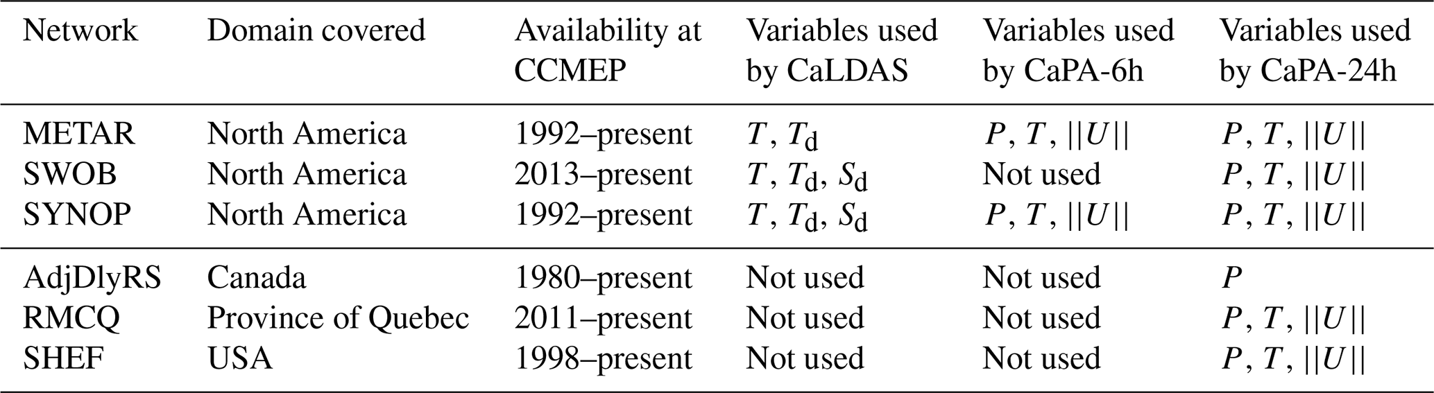
T: temperature, T_d: dew point temperature, S_d: snow depth, P: total precipitation, $\left|\right|U\left|\right|$: wind speed.

In order to improve the 24 h a posteriori precipitation analysis, supplementary quality controlled observations were pulled from ECCC's climate observations archive. These observations are available as part of the so-called Adjusted Daily Rain and Snow (AdjDlyRS) observations dataset (Wang et al., 2017). These observations were adjusted for systematic errors and in particular undercatch and evaporation caused by wind effects, gauge-specific wetting loss, and for trace precipitation amounts. This recently released dataset, which features 3346 stations, is considered one of the most accurate sources of retrospective precipitation data in Canada. AdjDlyRS stations are mainly based on manual stations from the Canadian synoptic network, which are known as the most reliable observations. For this reason, stations belonging to the AdjDlyRS dataset are not filtered out by CaPA's quality control for solid precipitation measurements. Observations from all other datasets are subject to this procedure, which has been shown to considerably improve the bias (Lespinas et al., 2015).

Table 3 summarizes the surface observation datasets used by CaLDAS and those used by CaPA for the 6 h analysis coupled to CaLDAS (CaPA-6h), as well as for the 24 h a posteriori precipitation analysis (CaPA-24h).

2.6 Additional surface observations used for evaluation purposes

Additional surface observations were used in order to evaluate precipitation, snow, and runoff predicted by the RDRS. For precipitation, two observation-based products were selected. The first product comprises 24 h precipitation accumulations over the United States obtained from the National Centers for Environmental Prediction's Stage IV analysis. The Stage IV analysis is a national product mosaicked from regional multisensor (radar + gauges) precipitation estimates (MPEs) produced by the 12 River Forecast Centers of the National Weather Service (Lin and Mitchell, 2005). Its resolution of 4 km is better than that of the RDRS, and thus is expected to provide more details about precipitation over the United States than the RDRS, but it does not cover neither Canada nor Mexico, and is not valid over water. The second product is version 2.3 of the Global Precipitation Climatology Project (GPCP), which is a global monthly product available on a 2.5×2.5^∘ grid, and thus covers the whole domain of interest, but at much lower resolution than the RDRS. It merges gauge and satellite data into a seamless product (Adler et al., 2003, 2018). For snow depth, density and water equivalent, a comprehensive Canadian database of snow surveys was selected (Brown et al., 2019).

For the evaluation of runoff, a Canada-USA transboundary watershed was selected: the Lake Erie watershed. Lake Erie, the tenth largest freshwater lake in the world by area, straddles the Canada-US border. It is part of the Laurentian Great Lakes system (Fortin and Gronewold, 2012), receiving water from Lake Michigan-Huron and draining into Lake Ontario through Niagara Falls. Its level has been steadily increasing since 2013, leading to frequent flooding in recent years (Gronewold and Rood, 2019), and is thus the subject of many studies looking at better predicting its water balance, such as the Great Lakes Intercomparison Project for Lake Erie (GRIP-E; Mai et al., 2021). Its watershed, defined as the land draining between Port Huron, at the outlet of Lake Michigan-Huron, and Niagara Falls, covers and area of approximately 78 000 km². Note that this watershed includes lands that drain into Lake Erie through the smaller Lake St. Clair. Inflows into Lake Erie from its watershed is not measured directly, but is estimated based on gauged tributaries using the area-ratio method (Fry et al., 2013). Streamflow gauge data were obtained from the United States Geological Survey (USGS) and the Water Survey of Canada (WSC) over the years 2010 through 2014 for 31 gauges located on rivers that drain into Lake Erie. The gauges were selected by Mai et al. (2021) as part of a hydrological model intercomparison study.

2.7 Verification metrics

Various verification metrics are used throughout the paper to evaluate prediction errors. Let X_n be a prediction, O_n the verifying observation, and $\mathit{\{}{\mathit{ϵ}}_n=O_n-X_n,n=\mathrm{1}$, …, N} a set of prediction errors. Commonly used metrics include the bias of the error, the standard deviation of the error (or STDE), the root mean square error (or RMSE) and the mean absolute error (or MAE):

$$\begin{array}{}\text{(1)}& \begin{array}{rl}& \mathrm{Bias}={\displaystyle \frac{\mathrm{1}}{N}}\sum _{n=\mathrm{1}}^N\left(\stackrel{\mathrm{‾}}{O}-\stackrel{\mathrm{‾}}{X}\right)={\displaystyle \frac{\mathrm{1}}{N}}\sum _{n=\mathrm{1}}^N{\mathit{ϵ}}_n=\stackrel{\mathrm{‾}}{\mathit{ϵ}},\\ & \mathrm{RMSE}=\sqrt{{\displaystyle \frac{\mathrm{1}}{N}}\sum _{n=\mathrm{1}}^N{\mathit{ϵ}}_n^{\mathrm{2}}},\\ & \mathrm{STDE}=\sqrt{{\displaystyle \frac{\mathrm{1}}{N}}\sum _{n=\mathrm{1}}^N{\left({\mathit{ϵ}}_n-\stackrel{\mathrm{‾}}{\mathit{ϵ}}\right)}^{\mathrm{2}}}=\sqrt{{\mathrm{RMSE}}^{\mathrm{2}}-{\mathrm{Bias}}^{\mathrm{2}}},\\ & \mathrm{MAE}={\displaystyle \frac{\mathrm{1}}{N}}\sum _{n=\mathrm{1}}^N\left|{\mathit{ϵ}}_n\right|.\end{array}\end{array}$$

where $\stackrel{\mathrm{‾}}{O}$ (resp. $\stackrel{\mathrm{‾}}{X}$) is the arithmetic mean of the observations (resp. forecasts). Note that bias is defined as being positive when the mean of the observations is larger than the mean of the predictions. The ideal value for all of these scores is zero.

Streamflow predictions are compared to observations using the Nash–Sutcliffe efficiency (NSE):

$$\begin{array}{}\text{(2)}& \mathrm{NSE}=\mathrm{1}-{\displaystyle \frac{\sum _{n=\mathrm{1}}^N{\left(O_n-X_n\right)}^{\mathrm{2}}}{\sum _{n=\mathrm{1}}^N{\left(O_n-\stackrel{\mathrm{‾}}{O}\right)}^{\mathrm{2}}}}.\end{array}$$

The ideal value for NSE is one; values above zero indicate better skill than climatology.

Precipitation predictions are compared to observations mainly through categorical scores. For a given threshold T, the number of hits H, misses M and false alarms F are defined as follow:

$$\begin{array}{}\text{(3)}& \begin{array}{rl}& H=\mathit{\#}\left\{\left(O_n>T\right)\bigwedge \left(X_n>T\right)\right\},\\ & M=\mathit{\#}\left\{\left(O_n>T\right)\bigwedge \left(X_n\le T\right)\right\},\\ & F=\mathit{\#}\left\{\left(O_n\le T\right)\bigwedge \left(X_n>T\right)\right\},\end{array}\end{array}$$

where # denotes the cardinal of the ensemble. From H, M and F, the probability of detection (POD), the false alarm ratio (FAR), the frequency bias index (FBI) and the equitable threat score (ETS) are defined as follow:

$$\begin{array}{}\text{(4)}& \begin{array}{rl}& \mathrm{POD}=H\cdot (H+M{)}^{-\mathrm{1}},\\ & \mathrm{FAR}=F\cdot (H+F{)}^{-\mathrm{1}},\\ & \mathrm{FBI}=(H+F)\cdot (H+M{)}^{-\mathrm{1}},\\ & \mathrm{ETS}=\left(H-H_{\mathrm{c}}\right)\cdot {\left(H+M+F-H_{\mathrm{c}}\right)}^{-\mathrm{1}},\end{array}\end{array}$$

where $H_{\mathrm{c}}=(H+F)\cdot (H+M)/N^{\mathrm{2}}$ is the number of hits expected by chance alone. The ideal value for FAR is zero, and it is one for POD, FBI and ETS.

In addition to these categorical scores, the partial mean of both observations and forecasts are compared in order to assess bias as a function of precipitation intensity. The partial mean (PM) of a sample $\mathit{\{}{X}_n,n=\mathrm{1}$, …, N} for a threshold T is defined as the arithmetic mean of sample values that are smaller or equal to T. As the threshold increases towards the largest value of the sample, the partial mean converges to the arithmetic mean of the sample. The ideal value of PM for a forecast is the partial mean of the observations for the same threshold.

3 Impact of surface assimilation

The impact of surface assimilation on the quality of the reanalysis was assessed using the RDRS-15 configuration (see Table 2). Although this version was run from 2010 to 2014, the evaluations were carried out on much shorter periods, more precisely the 2011 winter and 2011 summer periods, as well as the years 2013–2014. It is worth noting that the 2011 winter and 2011 summer have also been used by CCMEP to evaluate and validate all the forecast and analysis systems which were operational in 2015–2016, thus facilitating the comparison with the systems that were operational at that time.

In the following subsections, RDRS is evaluated against other reference experiments and datasets. As a general rule, surface analyses are not directly evaluated since all available observations were assimilated. The short-term forecasts that are part of the surface reanalysis creation process are evaluated instead. Evaluation of these short-term forecasts is also important, because these data are often used to force offline surface, hydrology and environmental models over long periods. The only exception to this rule is for precipitation. In that case, the precipitation analysis itself is evaluated, using a cross-validation procedure presented in detail by Lespinas et al. (2015).

A main reference in these evaluations is the RDPS, i.e. the operational regional weather forecasting system from CCMEP. The horizontal resolution of RDPS has increased over time but has remained at 10 km since October 2012. Indeed, considering that both systems (RDRS and RDPS) are based on the same atmospheric and surface models (GEM plus ISBA), results of the reforecast are expected to be in line with the latter and in particular should feature similar error signatures. The objective is not to obtain better results with RDRS than with RDPS, since RDPS is initialized with an in-house analysis developed for the latter on its native vertical coordinate and at higher resolution (both vertical and horizontal) and is using more advanced data assimilation method than what was used for ERA-Interim. The objective is rather to obtain forecasts of comparable quality for earlier years, with a system that can be more easily run from 1980 to the present day.

In order to assess the impact of land data assimilation on the quality of the resulting reanalysis, three RDRS-15 configurations are compared to RDPS and to each other: one in which surface initial conditions are provided by CaPA and CaLDAS (RDRS-15, also referred to RDRS + CaLDAS for clarity in the context of this comparison), one in which surface initial conditions are provided by GEM-Surf running in open-loop mode and forced by ERA-Interim (RDRS + Open-Loop), and one in which surface initial conditions are cycled, each run starting from a 12 h forecast of surface conditions obtained from the previous run of RDRS-15 (RDRS + Cycle). Surface initial conditions in RDRS + CaLDAS and RDRS + Open-Loop benefit from the assimilation (either through CaLDAS or ERA-Interim) of surface observations. On the other hand, RDRS + CaLDAS and RDRS + Cycle benefit from the fact that the same atmospheric model is used to drive the land-surface model in analysis and forecast mode. Only RDRS + CaLDAS has both features but is more costly to operate. RDRS + Open-Loop is closer to the dynamical downscaling approach used in a NWP context (with initial conditions coming from an independent analysis), and RDRS + Cycle is close to the dynamical downscaling approach used for regional climate modelling (with initial conditions obtained from a previous cycle of the limited area model).

Verifications are performed against radiosonde observations as well as surface observations from synoptic stations in North America. Comparing these three systems at the initial integration time would only inform us on the fit to observations of these systems, since these are not independent observations. Forecasts with lead times of 6 to 24 h are compared instead.

3.1 Impact of surface assimilation on the free atmosphere

In this first evaluation, results from the whole atmosphere are evaluated against radiosonde balloon observations that are launched twice a day (00:00 and 12:00 UTC) across the whole North American subcontinent in order to assess upper-air conditions. In particular, absolute temperature T, dew point temperature T_d, dew point depression T−T_d, wind speed $\left|\right|U\left|\right|$ and geopotential height Z_geop as a function of atmospheric pressure are evaluated. This methodology is standard at CCMEP and represents generally one of the very first steps when evaluating atmospheric systems. The same methodology is thus applied here. It is noteworthy that balloon vertical height measurement has historically been based on the environment pressure. Hence, each balloon's measurement is not located at the same height above ground level (a.g.l.) or above sea level (a.s.l.) but rather reported at standard pressure levels. As a result, comparisons with model outputs are also done based on pressure levels. While such an approach is convenient and straightforward for the free atmosphere, results obtained close to the surface have to be interpreted with caution: the lowest measurement of each balloon depends on the local surface pressure of its launching location (which is strongly correlated with the height a.s.l.). Thus, surface error is not only represented by the lower point of the profiles but spanning across the bottom of the profile (i.e. from 1000 up to 850 hPa).

Figure 4a shows comparison results for February/March 2011 and Fig. 4b shows results from the same approaches for July and August 2011. Comparisons are done after 24 h integration of the atmospheric model for the whole North America and results from the runs starting at 00:00 and 12:00 UTC are combined. In each of the panels the curves on the left show the bias while the curves on the right show the STDE.

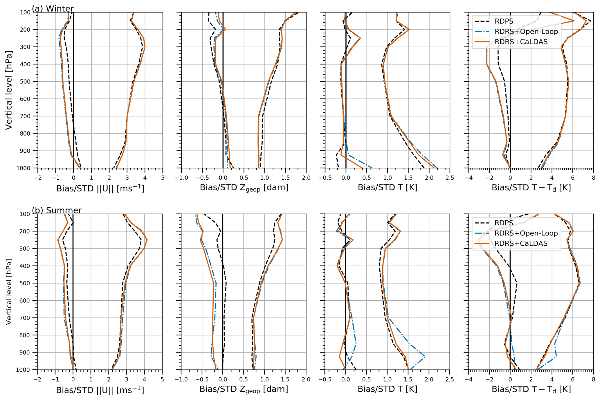
Figure 4 Comparison of atmospheric results from operational RDPS (black dashed line), RDRS + Open-Loop (blue dashed–dotted line) and RDRS + CaLDAS (orange continuous line) after 24 h integration against radiosonde for the whole North America (from left to right: wind modulus, geopotential height, absolute temperature, dew point depression): (a) February and March 2011; (b) July and August 2011. In each of the panels the curves on the left show the bias while the curves on the right show the STDE.

GEM integrations that are initialized with surface open-loop results forced by ERA-Interim (blue dashed–dotted line) are compared with integrations initialized with the CaLDAS analysis produced with the coupled system (orange continuous line). In both cases the atmosphere is initialized directly with ERA-Interim. It is noteworthy that the coupled system was run starting in January 2010 in order for the surface fields and notably the root zone water content to be properly initialized. In this figure, the operational RDPS results (2011 final cycles) are also shown as a reference (black dashed line) since the forecast component (GEM) of this system is very similar to the one used to produce the reanalysis.

The CCMEP analysis used to initialized the RDPS is much closer to the upper-air observations than ERA-Interim (not shown here), but this does not translate into a major advantage for the RDPS in the STDE of the forecast after 24 h of integration, as the weather systems have had time to evolve during the integration.

From Fig. 4a, it can be seen that during the winter the continuous orange lines and the dotted–dashed blue lines are very close to one another. Hence, results are almost unaffected by surface initialization, and only absolute temperature features small improvements (mostly for the bias) for the coupled reforecast compared to the uncoupled one. In the boundary layer, winter results are also generally in good agreement with the operational RDPS, with the exception of a warm bias and increased STDE of temperature and dew point depression below 850 hPa, which are both seemingly caused by initial surface conditions. The whole atmosphere is also wetter (as illustrated by a negative bias in dew point depressions) with a decreased wind modulus while the geopotential height is closer to the observations than the RDPS for both reforecast experiments, which is likely to be caused by ERA-Interim initial condition.

During the summer on the contrary, Fig. 4b, important differences between the two reforecast experiments can be observed in the temperature and dew point depression between RDRS + CaLDAS and RDRS + Open-Loop while both the wind modulus and geopotential height are almost unchanged. The coupled system, which is in very good agreement with the operational RDPS, shows great improvements over the open-loop initialized results, with an impact up to 700 hPa on both the temperature and dew point depression. Indeed, an important error develops in the uncoupled reforecast with a local maximum at 900 hPa. The shape and curvature of the bias for these two variables are also significantly different from the coupled approach (with the latter being more consistent with the RDPS): a warm dry bias develop above 1000 and up to 700 hPa in the uncoupled reforecast. These increased errors could be due to an inconsistency caused by the differences between GEM-Surf driven by ERA-Interim and GEM.

By further exploring these scores in details for the various run hours, lead times and geographical regions (not shown here), these errors turned out to be clearly increasing during summer afternoons inland, i.e. in places where convective instabilities driven by the sun heated surface dominate the diurnal cycle. This points to a deficient liquid water content in the soil at initialization, preventing a proper onset of latent heat flux and evapotranspiration and causing the atmosphere close to the ground to become too dry and hot in the open-loop initialized experiment. Figure 4 thus clearly illustrates the impact of land-surface and precipitation assimilation on the whole atmosphere.

From this first evaluation, it can be concluded that the coupled reforecast approach leads to atmospheric results which are more in line with the operational model for both seasons. They are always closer to the latter as well as observations vertically across the atmosphere than results from the reforecast initialized by the open-loop approach. This shows that the proposed approach is not only capable of performing properly in the boundary layer but also in the upper-air, demonstrating that the use of high-quality global atmospheric reanalysis such as ERA-Interim coupled with a land-data assimilation system can alleviate some of the cost of performing a regional reanalysis, since it is not necessary to perform a costly atmospheric assimilation procedure in order to obtain initial atmospheric conditions.

3.2 Impact of surface data assimilation on surface fields

Following the above atmospheric comparisons, this section aims to evaluate the very same winter and summer 2011 experiments but based on 2 m a.g.l. absolute and dew point temperatures as well as wind speed observations from the SYNOP network in North America. Table 4 summarizes the differences between RDRS + Open-Loop 24 h and RDRS + CaLDAS integrations in terms of averaged RMSE changes (in %) for various geographical subdomains. Cell values are shown in bold when a difference of more than 10 % is observed. Negative values, corresponding to cases where RDRS + CaLDAS is worse than RDRS + Open-Loop, are underlined.

Table 4 Summary of average changes (in %) of RMSE (against SYNOP observations) between RDRS + Open-Loop and RDRS + CaLDAS for February and March 2011 and July and August 2011. For each season, two columns show results from 24 h integrations starting at either 00:00 or 12:00 UTC. Changes of more than 10 % are shown in bold; negative values are underlined.

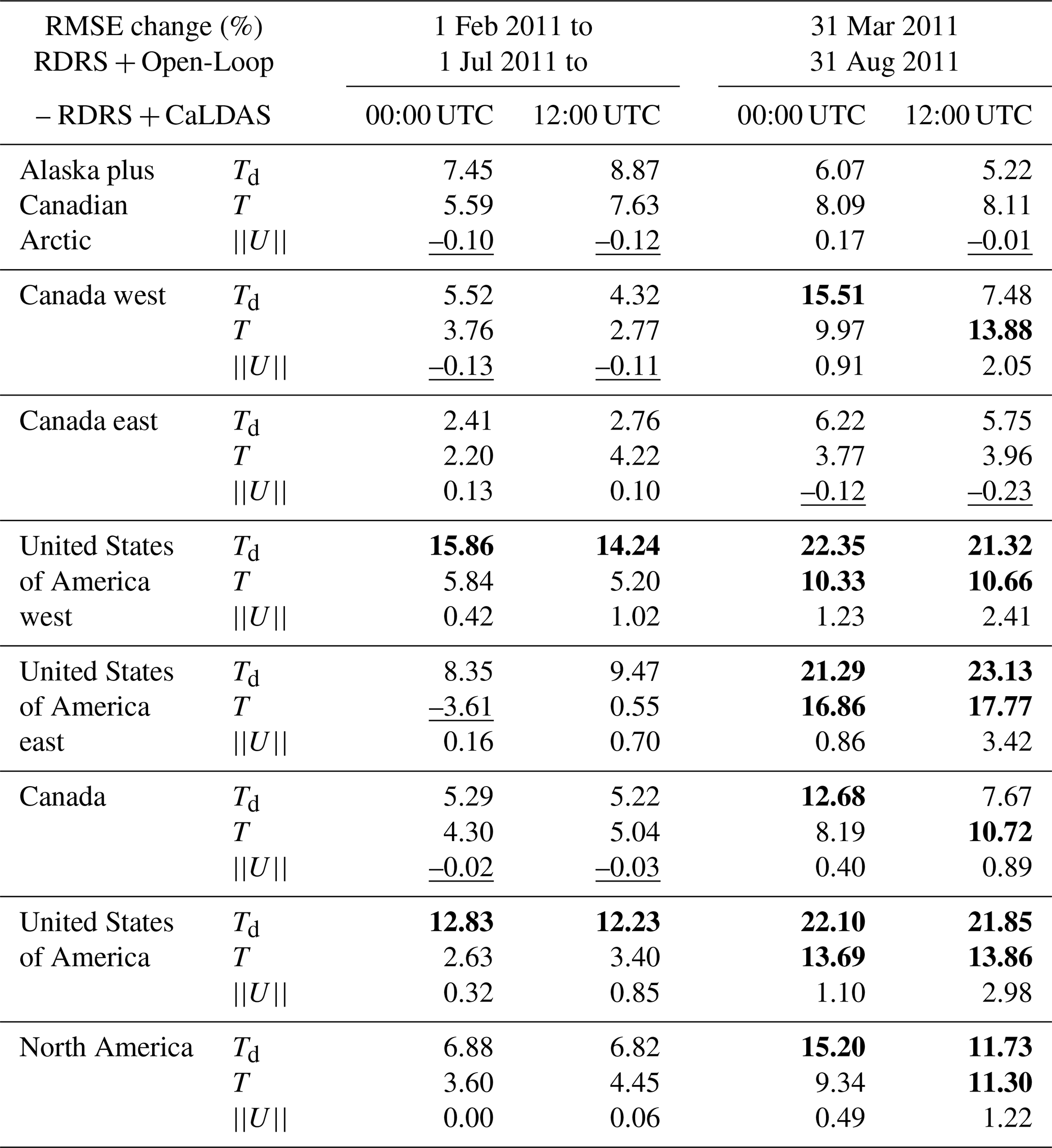
At the surface, the coupled reforecast approach almost always shows better results for absolute and dew point temperatures than simulations initialized with the open-loop regardless of the run hour or geographic domain. With the exception of integration starting at 00:00 UTC for the eastern USA domain in winter, absolute and dew point temperatures from RDRS + CaLDAS are always better by at least a couple of percent, and these improvements go up to 23 % in the eastern part of the USA for the summer. Generally, improvements are larger in summer than in winter. Concerning the wind modulus, differences are most of the time small. Nonetheless, wind modulus for USA domains in the summer show improvements on the order of a couple of percent.

Similar differences are obtained for integrations initialized at either 00:00 or 12:00 UTC. However, improvements for dew point temperature tend to be larger in summer for integrations initialized (and valid) at 00:00 UTC, i.e. in the evening for North America.

Instead of relying on initial surface conditions from an open-loop run, a second alternative to RDRS + CaLDAS is considered in which initial conditions are obtained through cycling: in the RDRS + Cycle experiment, GEM forecasts are initialized at the surface from the output of the previous model run, without any form of land-data assimilation. While this setup provides more consistency between the atmospheric and land-surface prediction, there is a risk of surface model drift, especially when running over such a large domain as North America. A longer model spin-up is also required in order for the root-zone water content to be properly initialized. However, if this approach were sufficiently accurate compared to RDRS + CaLDAS, it would be simpler to set up and less costly to run.

This approach was thus applied for a period of more than 2 years (2013–2015) and results obtained are illustrated based on STDE and bias in Fig. 5. In order to summarize 2 years of data, monthly averages of bias and STDE are computed, considering forecasts with lead times of 6 to 17 h. These are the lead times typically recommended for continuous offline simulation of surface and hydrology models: the first 6 h of each forecast is discarded to minimize model spin-up issues, and the next 12 h from both the 00:00 and the 12:00 UTC runs are combined to obtain a continuous hourly forcing dataset.

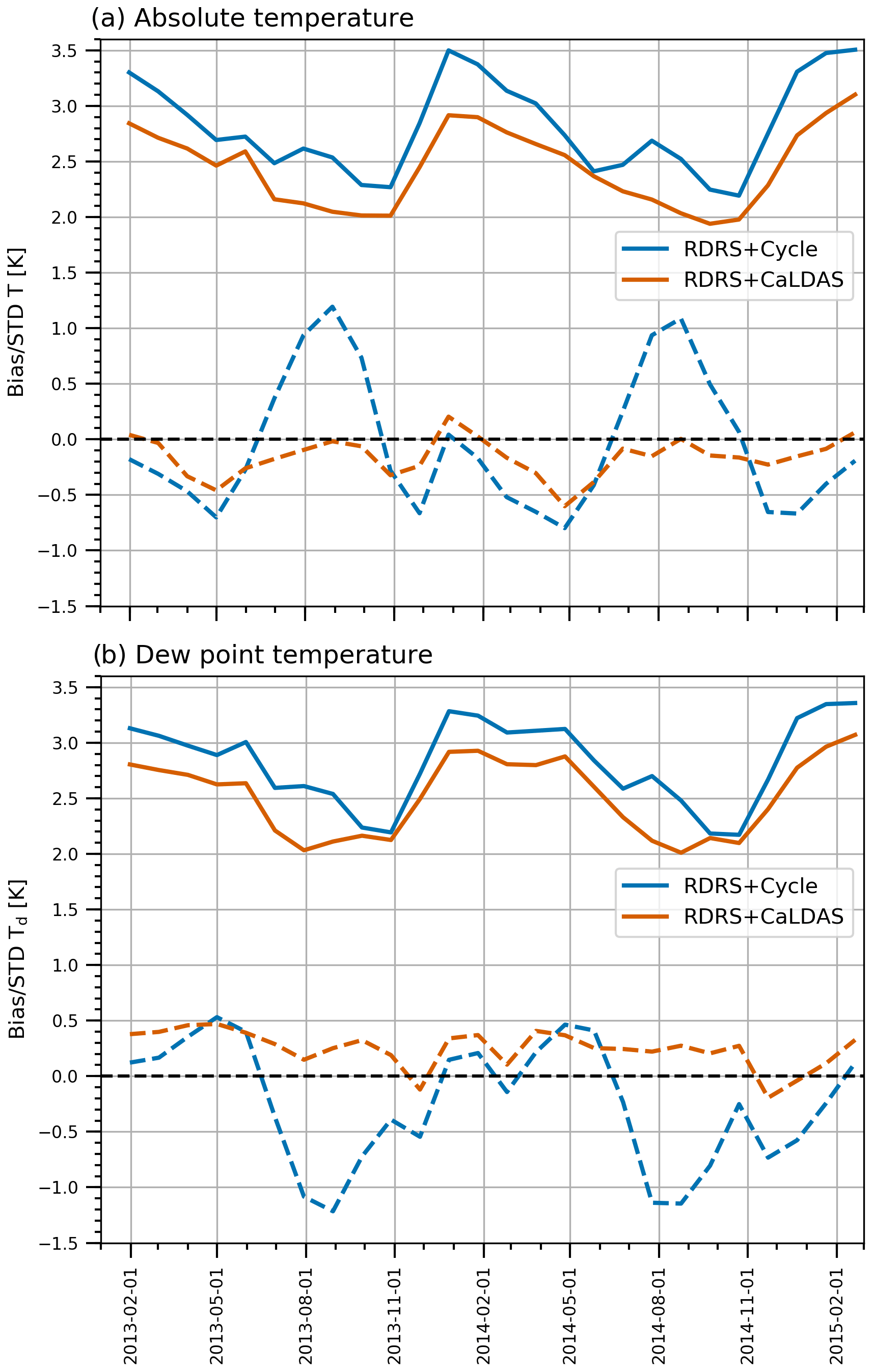
Figure 5 Comparison of reforecast surface results from RDRS + Cycle (blue) and RDRS + CaLDAS (orange) against SYNOP observations in terms of STDE (top curves, solid lines) and bias (bottom curves, dashed lines) computed based on monthly intervals for the whole North America and the 2013–2014 years: (a) absolute temperature; (b) dew point temperature. Results based on a combination of 6 to 17 h lead time from integrations starting at 00:00 and 12:00 UTC.

In that figure, the two plots present the STDE (top curves, solid lines) and the bias (bottom curves, dashed lines) for absolute temperature (top plot) and dew point temperature (bottom plot). The blue curve (resp. orange curve) corresponds to the RDRS + Cycle (resp. RDRS + CaLDAS) experiment. We can see that the coupled approach is always better for both the bias and STDE regardless of the season. The cycling approach also features degraded results in comparison to the RDRS + Open-Loop (not shown here). Most notably, during the summer months, the approach where the surface is cycled shows an important increase of the absolute temperature bias along with an important decrease of dew point temperature bias. This tends to point out that there is not enough water available in the soil for evaporation causing a warmer and dryer atmosphere close to the ground. Indeed, at these resolutions and when relying on the cold-start diabatic filter for initialization, GEM requires a spin-up period of at least 6 h for its precipitations to reach a stable level. This deficit of water can be partly explained by the fact that the surface scheme implemented in GEM-Surf, i.e. ISBA, is recognized not to properly retain soil moisture (Alavi et al., 2016). This model deficiency is compensated by CaLDAS through positive increments in soil moisture. During winter, while results from the coupled approach tend to be closer to the observations for both bias and standard deviation, differences are not as important as for the summer season.

Results presented in the above two sections clearly show the added value of the coupled approach with regards to the surface layer and atmosphere. Results obtained are in line with the operational model in the atmosphere. In the surface layer, significant improvements are obtained in comparison with the simpler and more standard open-loop or cycling approaches. It is based on these results that the production of a 10 km configuration of the RDRS, coupled with CaLDAS, was launched at CCMEP for the period 1980–2018. The next section presents an evaluation of this product for surface variables, precipitation accumulations and streamflow.

4 Evaluation of the continuous hourly forcing dataset over 2011–2017

The impact of surface and precipitation analysis on reforecasts has been evaluated on short time periods in the previous section. An improvement of the reforecast is observed when the RDRS is coupled with the RSAS analysis system (based on CaPA and CaLDAS). The present section aims to evaluate various aspect of the reanalysis over a longer time period (2011–2014 for RDRS-15 and 2011–2017 for RDRS-10) in order to better appreciate its quality. Comparison against screen-level absolute and dew point temperatures, wind speed, precipitation, and streamflow in situ observations are presented, followed by a comparison of precipitation totals with other products available for North America.

Furthermore, the evaluation is focused on the continuous hourly forcing dataset recommended for offline simulation of surface and hydrology models, which will be distributed to stakeholders as the main outcome of this project. For absolute temperature, dew point temperature, humidity, radiation, wind speed and pressure, this dataset is obtained by combining RDRS forecasts with lead times of 6 to 17 h from both the 00:00 and the 12:00 UTC runs. For precipitation, the CaPA-24h product, disaggregated to a hourly time step, is used (see Sect. 2.3). The resulting datasets are referred to in this section simply as RDRS-15 and RDRS-10 or else as RDRS-15 + CaPA-24h and RDRS-10 + CaPA-24h when precipitation or offline hydrological simulations are evaluated.

4.1 Absolute temperature, dew point temperature and wind speed

This section focuses on the evaluation of the RDRS-15 and RDRS-10 short-term forecasts (with lead times of 6 to 17 h) against absolute and dew point temperature observations from synoptic stations in North America. Initial surface conditions for the RDRS-15 and RDRS-10 are provided in all cases by CaLDAS. The performance of the RDPS which was operational at the time is also shown as a reference.

Figure 6 presents the time evolution of the RMSE for the RDRS-15 (continuous orange line), RDRS-10 (dashed–dotted blue line) and RDPS products (black dashed line), assessed against all SYNOP observations located in North America. A monthly time interval is used to compute error statistics. A clear annual cycle is observed, with errors being generally larger in winter and spring, and smaller in summer and autumn. Errors in absolute temperature forecasts (Fig. 6a) and dew point temperature forecasts (Fig. 6b) show similar patterns. While RDRS-15 and RDRS-10 errors behave similarly, RDPS errors are larger for the earlier years. Focusing on dew point temperature forecast errors (Fig. 6b), it can be seen that the differences between RDPS and RDRS errors become smaller starting in 2015 and are very similar after mid-2016. For wind speed (Fig. 6c), RDPS and RDRS-15 errors are very similar until the end of 2014, and slightly smaller in winter for RDPS after this date.

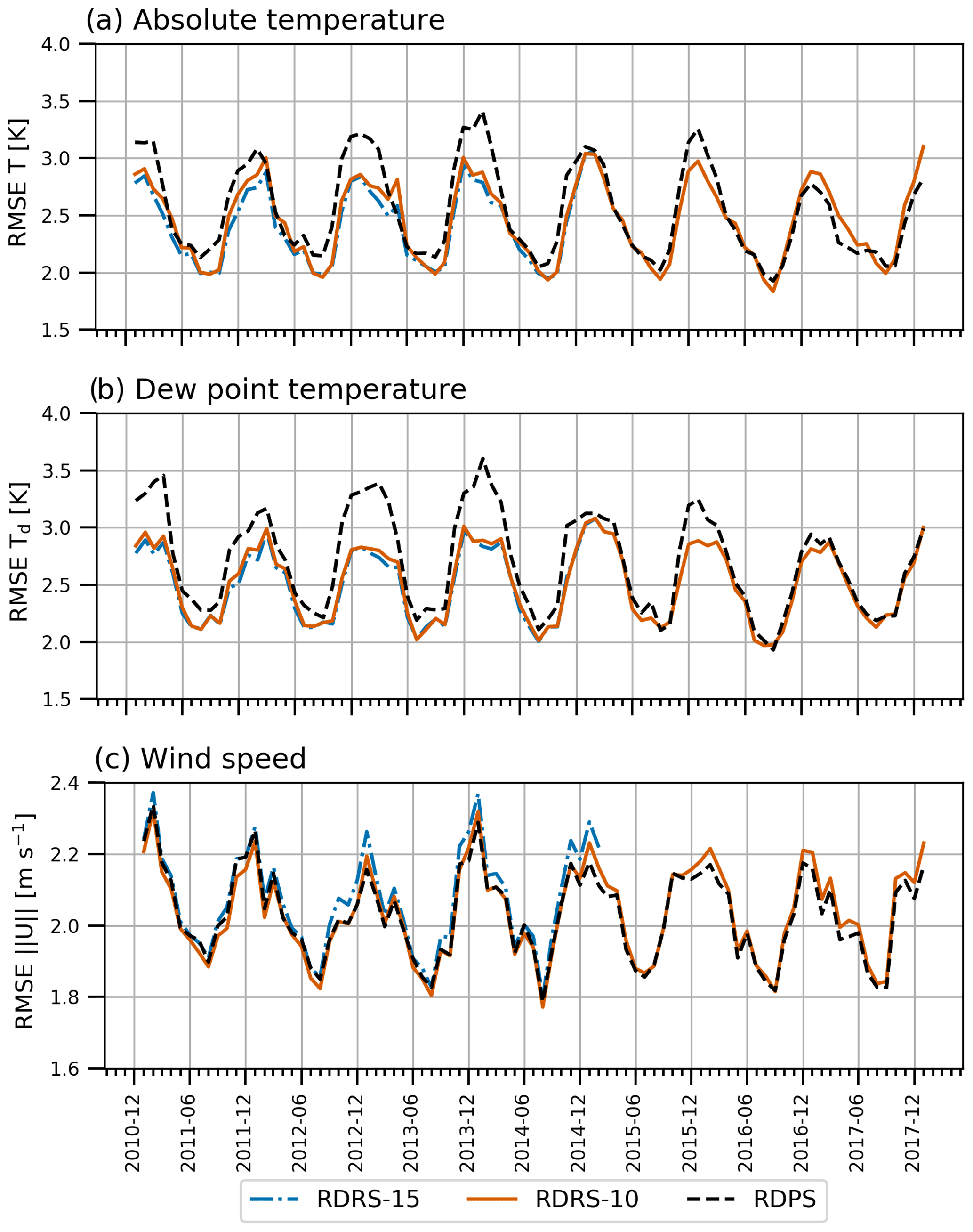
Figure 6 Time series of RMSE (against SYNOP observations) from operational RDPS (black dashed line), RDRS-10 (orange continuous line) and RDRS-15 (blue dashed–dotted line) computed based on monthly intervals for the whole North America and the 2011–2017 years: (a) absolute temperature; (b) dew point temperature; (c) wind speed. Results only based on a combination of 6 to 17 h lead time from integrations starting at 00:00 and 12:00 UTC.

The reduction of errors in RDPS forecasts (when compared to both RDRS-15 and RDRS-10) at the end of 2014 and again in mid-2016 is likely the consequence of changes to the operational version of RDPS. In fact, a major upgrade to the data assimilation system was implemented on 18 November 2014 (Caron et al., 2015), and a major upgrade to the GEM model was implemented on 7 September 2016 (Caron et al., 2016). After this date and until the end of the evaluation period, the RDPS relied on the same version of GEM as the RDRS.

When comparing RDRS-15 and RDRS-10 over the whole North America, it can be noted that the 15 km configuration of the system has slightly smaller errors than the 10 km configuration for absolute and dew point temperatures and slightly larger errors for wind speed, although the differences are small in all cases and typically smaller than the differences between RDRS-15 and RDPS errors.

A regional evaluation of the performance of the RDRS is presented in Table 5, which summarizes the average changes in RMSE between RDRS-10 and RDRS-15 as well as between RDRS-10 and the operational RDPS by seasons and geographical domains. Scores are again computed against observations from the SYNOP network and based on forecasts with 6 to 17 h lead time. The time period for the evaluation is restricted to 2011–2014, during which outputs from all three systems are available.

Table 5 Summary by seasons of average changes (in %) of RMSE (against SYNOP observations) between operational RDPS, RDRS-10 and RDRS-15 for 2011–2014 years. For each season, results are based on a combination of 6 to 17 h lead time from integrations starting at 00:00 and 12:00 UTC. Changes of more than 10 % are shown in bold; negative values are underlined.

It can be seen that over this period, i.e. prior to the upgrade of the atmospheric data assimilation system and GEM model version of the RDPS, RDRS-10 improves upon RDPS in most regions and for most variables, notably for Alaska and the Canadian Arctic, as well as western USA. Absolute and dew point temperature forecasts are improved for all seasons and all domains, with the sole exception of absolute temperature in spring and summer for the eastern Canada domain. This degradation is caused mainly by errors in the sea surface temperature (SST) obtained from ERA-Interim: indeed, forecasts of similar skill are obtained for RDPS and RDRS when using operational CCMEP SST analyses (not shown). Improvements of more than 10 % are obtained in many cases. They are shown in bold in Table 5. For example, a 24 % reduction of forecast error is obtained for dew point forecasts over Mexico during the autumn season, and a 25 % reduction of forecast error is obtained for absolute temperature forecasts over western USA during the winter season. RDRS-10 wind forecast errors are slightly better than RDPS forecasts for all domains in the summer and autumn seasons, with the exception of Mexico during the summer season. During winter and spring, RDRS-10 wind forecasts are slightly better for the USA and in particular for the western half of the USA but slightly worse for Canada and Mexico. In all cases, differences in wind speed forecast errors do not exceed 2 %. When comparing RDRS-10 and RDRS-15 forecasts, it can be seen that RDRS-10 absolute and dew point temperature forecasts are generally worse, with the exception of dew point temperature forecasts over Mexico. On the other hand, RDRS-10 wind forecasts are better than RDRS-15 forecasts for all domains and seasons. All of the differences between RDRS-10 and RDRS-15 RMSE are fairly small. The most important RMSE change being −4 % for dew point temperature (USA west domain, winter season), −6 % for absolute temperature (Canada east domain, spring season), and +4 % for wind speed (Canada east domain, winter season).

Overall, this evaluation suggests that RDRS-10 near-surface forcing data should be competitive with recent RDPS forcing data for driving surface, hydrology and environmental models, at least for absolute temperature, dew point temperature and wind speed.

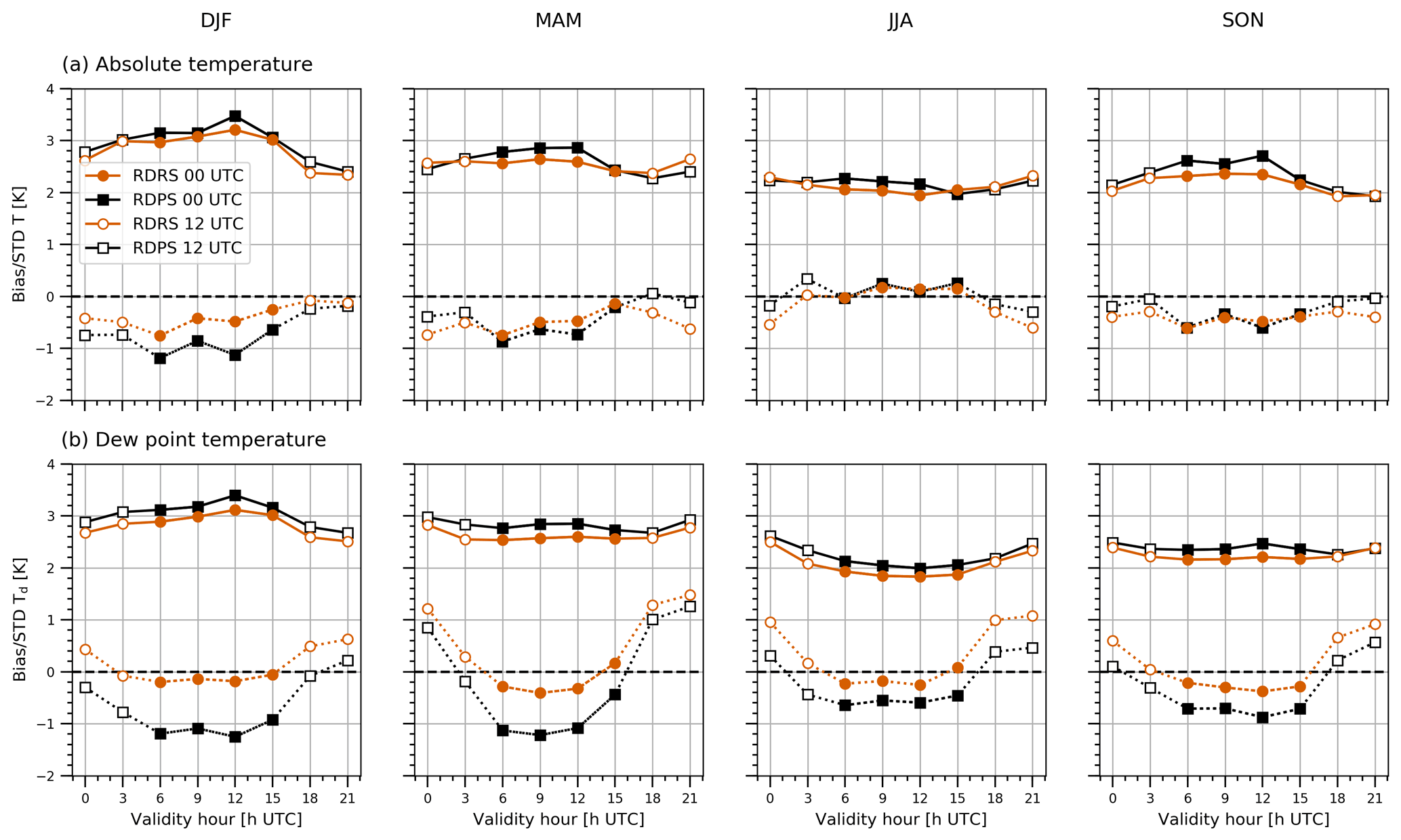
Figure 7 Seasonal diurnal cycles of surface results from operational RDPS (black with square markers) and RDRS-10 (orange with round markers) against SYNOP observations in terms of STDE (top curves, solid lines) and bias (bottom curves, dashed lines) for entire North America over the period 2011–2017; from left to right: winter (DJF); spring (MAM); summer (JJA); autumn (SON); (a) absolute temperature; (b) dew point temperature. Results are only based on the 6 to 17 h lead time from integrations starting at 00:00 UTC (filled markers) and 12:00 UTC (empty markers).

Although prediction skill is important for a reanalysis dataset, it is also important to assess the diurnal reanalysis bias, which is interesting by itself and also because it affects the RMSE of the reanalysis. The diurnal STDE is also interesting to assess, as it is equivalent to the RMSE of forecasts from which the bias has been removed. Figure 7 shows, for each season, the diurnal cycle of the bias and standard deviation of the RDRS-10 and RDPS errors assessed against all SYNOP observations located in North America. Each graph is based on 7 years of data (2011–2017). The first row of plots presents results for absolute temperature, and the second row presents results for dew point temperature. Each column corresponds to a different season. Each plot contains four curves: two for RDPS forecasts (in green) and two for RDRS-10 forecasts (in orange). The top two curves (filled lines) on each graph correspond to the STDE as a function of time of day (in UTC), whereas the bottom two curves (dashed lines) correspond to the bias. Model runs initialized at 00:00 UTC (resp. 12:00 UTC) are used for hours 06:00, 09:00, 12:00 and 15:00 UTC (resp. 18:00, 21:00, 00:00 and 03:00 UTC), with results shown using filled (resp. empty) markers.

In terms of standard deviation, RDRS-10 forecast errors are generally smaller than RDPS forecast errors, especially for 00:00 UTC forecasts valid from 06:00 to 15:00 UTC (filled markers), and hence during the night and early morning in North America. The error signature of both systems is fairly similar. In particular, errors are larger in winter than in summer; they are larger during the night and early morning during winter (forecasts issued at 00:00 UTC, filled markers) and generally larger during the afternoon and evening in summer (forecasts issued at 12:00 UTC, empty markers). The bias signature of both systems is similar for absolute temperature (first row of plots). The RDRS-10 winter absolute temperature bias is better than that of the RDPS for all hours of the day. For other seasons, the bias is slightly worse during the afternoon and evening hours and comparable during the night and early morning. For dew point temperature, the diurnal cycle of RDRS-10 and RDPS is very similar, but the RDRS-10 bias curve is always above the bias curve of the RDPS, which is an indication that the land-surface is wetter in the RDRS-10. During the night and early morning, this always corresponds to an improvement in the bias. During the afternoon and evening hours, the RDRS-10 bias is generally worse than the RDPS bias. Hence, environmental models that are particularly sensitive to humidity might behave differently when forced with RDRS-10 data compared to RDPS data.

4.2 Precipitation

Two strategies were considered in order to assess the precipitation reanalysis skill and bias at both 15 and 10 km: (1) seasonal accumulation maps were obtained for the CaPa-24h reanalysis at both resolutions and visually compared to Stage IV MPE (Lin and Mitchell, 2005) and GPCP (Adler et al., 2003, 2018) for each season of the period 2010–2014, and (2) verification scores routinely used for evaluating the operational CaPA precipitation analysis were computed over the same period for both reanalysis products but also for the background field used for each product.

4.2.1 Seasonal accumulation

Figure 8 compares the seasonal accumulations of precipitation for the two versions of the CaPA-24h reanalysis (at 15 and 10 km resolution) to the seasonal accumulations of precipitation estimated from Stage IV MPE and GPCP datasets. Each column corresponds to a season: spring (MMA), summer (JJA), autumn (SON) and winter (DJF). Each row presents accumulations for a different product: (a) CaPA-24h based on RDRS-10, (b) CaPA-24h based on RDRS-15, (c) Stage IV MPE and (d) GPCP. Of the four products, only GPCP provides global coverage. However, it can be seen that the domain covered by both versions of CaPA covers all of North America, including the coastal oceans. Stage IV MPE is limited to the conterminous US plus the Columbia river basin in British Columbia and the Rio Grande basin in Mexico.

Over the oceans, large differences are observed between the three products providing coverage: CaPA-24h is nearly identical to its background field, since very few observations are available to constrain the analysis. Thus, it is essentially the RDRS precipitation accumulations that are shown over the oceans in the first two rows of Fig. 8. It appears that the RDRS-15 precipitation matches better the GPCP precipitation, but both RDRS-15 and RDRS-10 seem to overestimate precipitation, in particular over the Gulf Stream. Difference over the ocean between RDRS-10 and RDRS-15 can be explained by the use of differing shallow convection parametrization: while the latter is closer to observation, it breaks conservation laws (Bélair et al., 2005). In the meantime, the overestimation of both approaches might be indicative of an excess of evaporation at mid-latitude in the GEM model, leading in turn to an excess of precipitation, as suggested by the evaluation performed by Deacu et al. (2012) over Lake Superior.

Figure 8 Precipitation accumulation per seasons [mm/month] over years 2010–2014 for (a) CaPA-24h based on RDRS-10; (b) CaPA-24h based on RDRS-15; (c) NOAA Multisensor Precipitation Estimates (Stage IV) 24 h analysis; and (d) Global Precipitation Climatology Project (GPCP) monthly analysis.

Over the USA, Stage IV and GPCP agree well for the larger-scale features, with Stage IV MPE providing more details. Even at 15 km, CaPA-24 also provides much more details than GPCP and generally agrees well with Stage IV MPE. However, CaPA-24h clearly lacks precipitation during the summer months in the southeast of the US. This is an area known for its strong convective storms in summer, and the associated precipitation is likely not well captured in neither the GEM model background field nor in the in situ observational dataset assimilated by CaPA. Over Canada, significant differences are observed between GPCP and CaPA-24, both in terms of precipitation accumulations and variability. This is expected, as neither product relies on a dense precipitation network (especially in northern Canada). Furthermore, the CaPA reanalyses assimilate datasets that are not considered by GPCP (such as the RMCQ network in the province of Quebec), as well as precipitation observations that have been corrected for known biases (the AdjDlyRS dataset).

4.2.2 Scores

In addition to a visual comparison of CaPA-24h reanalyses with reference precipitation products available over North America, an objective verification was also performed. Evaluating precipitation analyses is, however, more challenging than evaluating precipitation forecasts, since independent verification data are hard to come by, especially in regions with already sparse networks like northern Canada. One option is to rely on data-denial experiments. For CaPA operational analyses and reanalyses, leave-one-out cross-validation is routinely used, as it is a by-product of the in-line quality control procedure (Lespinas et al., 2015). Verification metrics generated by this procedure include the probability of detection (POD), the false alarm ratio (FAR), the frequency bias index (FBI) and the equitable threat score (ETS). It is also useful to compare the partial mean (PM) of the observations with that of the analysis in order to assess quantitative bias as a function of precipitation thresholds.

These different verification metrics are presented for each season in Fig. 9. Each row corresponds to a season (DJF, MAM, JJA and SON) and each column to a verification metric. The x axis is the precipitation threshold (in mm d⁻¹) for which the verification metric is computed, and the y axis corresponds to the value of that metric. For POD, FAR, FBI and ETS, four curves are shown on each graph. Continuous (resp. dashed) lines present the verification metrics for the reanalyses (resp. background field). Blue (resp. orange) curves correspond to the 15 (resp. 10) km products. In the last column, the partial mean of the observations is shown in black. It corresponds to the ideal value for the PM verification metric. For FBI, the ideal value of one is also highlighted using a black line.

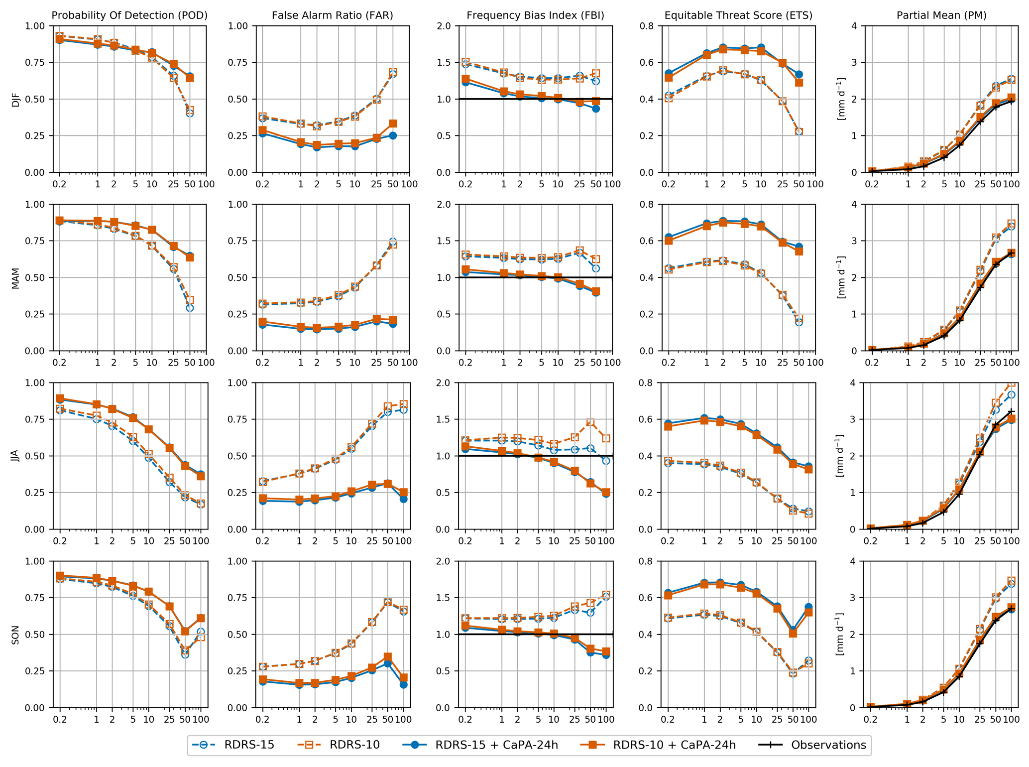
Figure 9 Comparison of CaPA-24h background field (dashed lines) and analyses (continuous lines) at 10 km (orange lines) and 15 km (blue lines) against manual synoptic stations over years 2010–2014. Each row corresponds to a season (winter, spring, summer and autumn) and each column to a score (probability of detection, false alarm ratio, frequency bias index, equitable threat score and partial mean). The x axis is the precipitation threshold [mm d⁻¹].

As these are generally considered more accurate, verification is performed against manual synoptic stations in the US and Canada plus climate stations from the AdjDlyRS dataset. Observations that do not pass the quality control of CaPA are discarded from the verification dataset in all cases.

It is clear from this figure that both analyses are more skilful (in terms of ETS) and less biased (both in terms of FBI and PM) than their background field. False alarms (FAR) are also significantly reduced in the reanalysis for all seasons and thresholds. The probability of detection (POD) in winter for thresholds of 2 mm d⁻¹ or less is the only score for which the reanalysis is worse than the background field. However, given the improvements in the FAR, FBI and ETS, this is deemed acceptable.

What is less clear is the added value of the 10 km compared to the 15 km products: the POD is similar or slightly improved, but the FAR is degraded, in particular for larger precipitation thresholds. The FBI is higher at 10 km resolution, which results in a degraded categorical bias for lower thresholds, but an improved categorical bias for higher thresholds. The ETS is almost always slightly worse at 10 km resolution. The PM is nearly identical at both resolutions. In summary, the 10 km is slightly less skilful than the 15 km reanalysis (as measured by the ETS), and this is due to an increased ratio of false alarms.

In general, the degradation in the FAR and ETS of the analysis when going from 15 to 10 km is not seen in the background field (with the notable exception of higher precipitation thresholds in summer). Furthermore, in most cases the difference in the scores of the two reanalyses is larger than the difference in the scores of the two background fields, which tends to be small. In spring, summer and autumn, the POD, FBI and PM of the background field are, however, generally higher at 10 km, reflecting a worsening of the positive precipitation bias already present at 15 km.

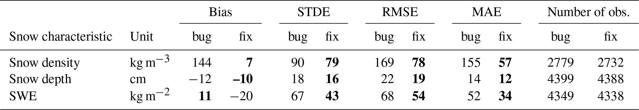
Table 6 Bias, STDE, RMSE and MAE of snow density, snow water equivalent (SWE) and snow depth computed from 1 January 2014 to 31 January 2015 with the bug and with the fix for the bug identified in the RDRS (and in the operational RDPS) when estimating the maximum value for snow density as a function of snow depth. Best score for each snow characteristic is shown in bold. Number of observations used for the evaluation is shown in the last two columns.

4.3 Snowpack

Snow depth and snow water equivalent (SWE) are of interest for surface and hydrological prediction. They are both routinely observed, but fewer automatic SWE measurements are available. Furthermore, SWE is often reported only around the 1st and 15th day of each month. In order to be able to compare the skill and bias of these two properties, verification was restricted to cases where both quantities were available in the Canadian historical snow survey database compiled by Brown et al. (2019). Only snow surveys taken at an altitude within 300 m of the atmospheric model topography were considered. The evaluation was performed over 1 January to 15 May 2014 and 15 November to 31 January 2015, since no observations were available during the warm season. Pairs of observations and corresponding analysis values were obtained at each site for the 1st and 15th day of each month, with a tolerance of ±6 d on the observation date in order to maximize the number of measurements used for the evaluation while avoiding over-representing the verification dataset stations reporting more often than once every 2 weeks. Indeed, manual snow survey sites are typically visited at most twice per month. Bias, STDE, MAE and RMSE were then computed for RDRS-10. While satisfactory results were obtained for SWE and snow depth, the performance was rather poor for snow density.

A code review revealed that an error had been introduced in the GEM model when implementing the parameterization for maximum snow density proposed by Bélair et al. (2003a). Indeed, Eqs. (21) and (22) in Bélair et al. (2003a) are valid for snow depth expressed in centimetres (cm), whereas snow depth is expressed in metres (m) in both the paper and the GEM code. In addition to being present in the reanalysis, this bug impacts all operational NWP systems based on GEM as of 2020. It will be corrected in future releases. In order to assess the impact of the bug fix, the surface reanalysis was relaunched for 2014.

Table 6 presents the bias, STDE, MAE and RMSE of snow density, snow depth and SWE with and without this bug fix. When using the correct implementation of the maximum snow density parameterization, the bias on snow density drops from 144 to only 7 kg m⁻³ and STDE is also lowered from 90 to 79 kg m⁻³. Consequently, RMSE is reduced from 169 to 78 kg m⁻³. MAE is also considerably reduced from 155 to 57 kg m⁻³. Modest improvements in snow depth predictions are, however, observed for all metrics: differences range from a 2 cm improvement for bias, STDE and MAE to a 3 cm improvement for RMSE. With the bug fix, the bias of snow depth predictions is −10 cm, STDE is 16 cm, MAE 12 cm and RMSE 19 cm. The impact on the bias and skill of SWE predictions is more important than for snow depth but not as important as for density. For SWE, the positive bias of 11 kg m⁻² obtained with the bug becomes negative and slightly worse (−20 kg m⁻²) with the bug fix. STDE is, however, improved from 67 to 43 kg m⁻². The net effect on RMSE is a reduction of the error from 68 to 54 kg m⁻². MAE is also improved with the bug fix from 52 to 34 kg m⁻².

4.4 Streamflow

In a first attempt to assess the suitability of the dataset for hydrological prediction, the GEM-Hydro model (Gaborit et al., 2017) was used to predict the inflows into Lake Erie. The land-surface of the GEM-Hydro model was set up on a 10 km grid, the routing was performed on a 1 km grid, and both were calibrated using the RDRS-15 + CaPA-24h forcing, using a methodology described in Mai et al. (2021), over the years 2011–2014 (2010 used for spin-up).

Figure 10 shows a comparison of the simulated inflows obtained when forcing the calibrated GEM-Hydro version with three different datasets: RDRS-15 + CaPA-24h, RDRS-10 + CaPA-24h and RDPS + CaPA-24h. Figure 10a shows the daily inflows from January 2011 to December 2014 obtained by aggregating the flows from all of the tributaries draining directly into Lake Erie. Figure 10b presents the same data as in Fig. 10a but ranked for lowest to highest value and using a log scale. Figure 10c shows the cumulative runoff over this 5-year period obtained for the observations and the model by summing up the daily inflows, dividing by the area of the watershed and converting units into metres.

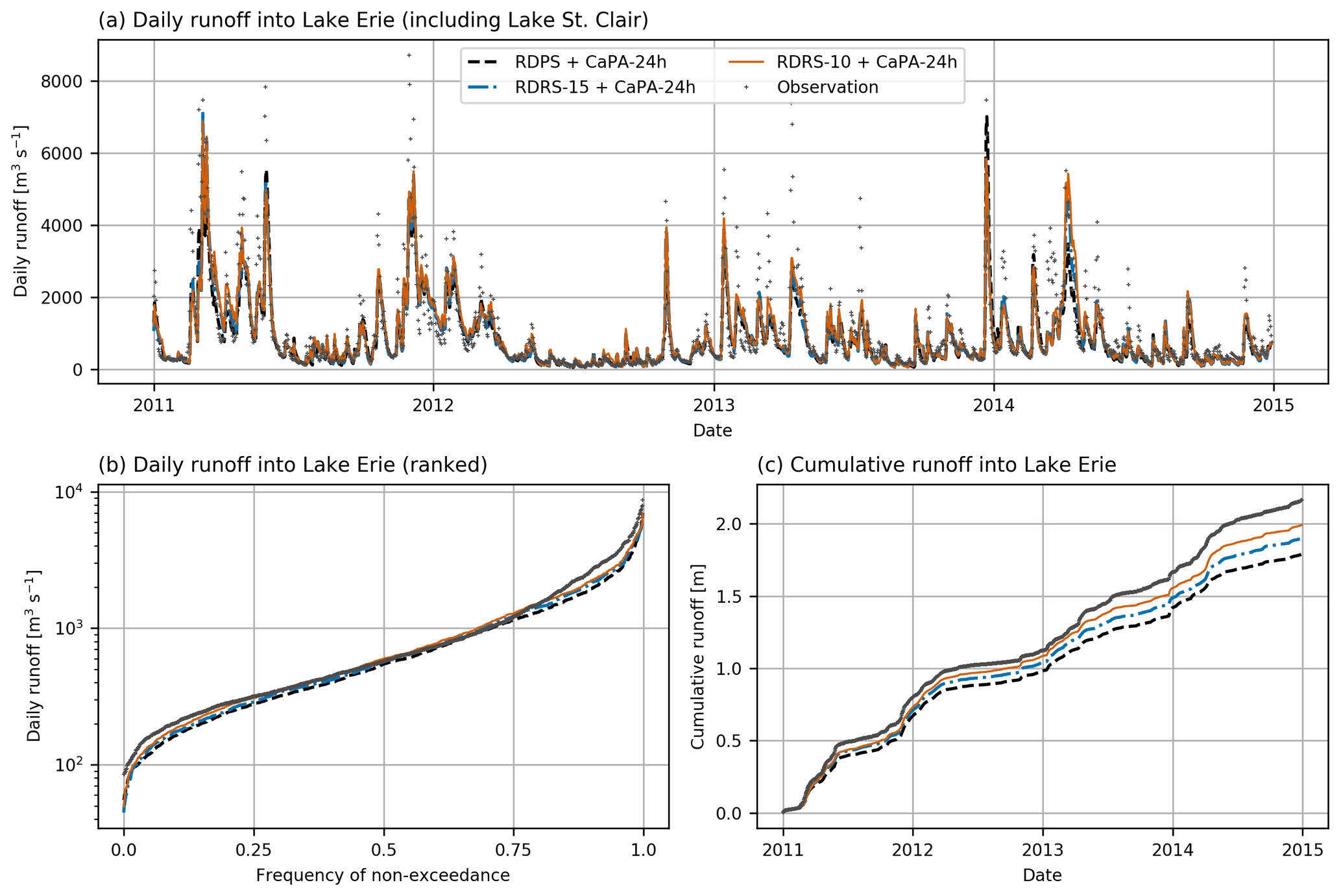
Figure 10 Comparison to observed Lake Erie inflows (grey dots) of GEM-Hydro simulations based on RDRS-10 + CaPA-24h (continuous orange line), RDRS-15 + CaPA-24h (dashed–dotted blue line) and RDPS + CaPA-24h (dashed black line) forcing for years 2011–2014: (a) daily inflows [m³ s⁻¹]; (b) ranked daily inflows, log scale [m³ s⁻¹]; and (c) cumulative inflow over the 5-year period [m].

The comparison between observed and modelled daily inflows (Fig. 10a) shows that GEM-Hydro is able to represent the dynamics of the watershed in periods of both low and high inflows for all three sets of forcing data. Nash–Sutcliffe efficiency (NSE) values over 2011–2014 (2010 was used for model spinup) for the three experiments are respectively 0.77 for RDRS-10 + CaPA-24h, 0.78 for RDRS-15 + CaPA-24h and 0.77 for RDPS + CaPA-24h. It is not surprising to obtain a slightly better NSE with the RDRS-15 forcing, since they were used to calibrate the model. Figure 10b shows that both low and high flows are negatively biased in all three simulations, even if the RDRS-10 + CaPA-24h dataset leads to slightly higher flows at both ends of the spectrum. The comparison between the observed and modelled cumulative runoff (Fig. 10c) is useful in assessing the bias of the simulations. It can be seen that better results are obtained in terms of cumulative runoff with the RDRS-10 + CaPA-24h forcing, followed by RDRS-15 + CaPA-24h. RDPS + CaPA-24h leads to more biased predictions, on the order of 17 %, compared to 12 % for RDRS-15 + CaPA-24h and 8 % for RDRS-10 + CaPA-24h. Remaining simulation errors can be partly explained by the presence of large agricultural and urbanized areas in the watershed (Mai et al., 2021). In particular, tile drains and impervious areas are not represented accurately in the model.

This analysis of simulated streamflow provides some evidence that the forcing data based on the RDRS can be useful for hydrological prediction and in particular for transboundary watersheds of North America. This is true even if the reanalysis is only available for a historical period. Indeed, models relying on NWP outputs typically require calibration in order to perform optimally, partly due to the errors/biases and shortcomings of their input datasets. This is particularly true for surface and hydrological models. Such a calibration can only be performed based on historical datasets that ideally have the same climatology as the product used to drive such models in a forecasting context. However, archived datasets from operational NWP models tend to evolve in time and are usually not available for time periods long enough for such a calibration exercise. Another important point worth mentioning is that hydrological models are not only used to predict future flows. For example, they can be used to predict past flows at ungauged locations, to infill missing data at gauged locations, and to perform what-if scenarios to assess the impact of climate change, land-use changes and reservoir regulation changes.

5 Discussion and conclusion

This paper presents and evaluates a methodology for minimizing the computational cost and the data processing burden associated with the production of an atmospheric reanalysis and still obtain consistent, high-quality and high-resolution atmospheric, surface and precipitation fields. A final precipitation analysis is then obtained in a postprocessing step in order to assimilate additional precipitation observations which significantly improves the quality – and local relevance – of the precipitation analysis. The methodology is used to obtain a first reanalysis based on the GEM model, which is at the heart of the operational NWP system used by the Meteorological Service of Canada. The reanalysis provides seamless coverage for all of North America and the Arctic Ocean at 10 km resolution and hourly time step, and it is of particular interest for hydrological applications in transboundary watersheds sitting on the Canada–US border. Results obtained when forcing a hydrological model in order to predict inflows into the Lake Erie watershed are encouraging.

5.1 Impacts of the land-data assimilation system on the reanalysis quality and production strategy

The various numerical experiments have shown the important role played by the land-data assimilation system in the quality of the product not only at the surface but also for the boundary layer. Indeed, using CaLDAS allows for better results for absolute and dew point temperatures in the boundary layer (cf. Fig. 4) and at the surface (cf. Fig. 5). Initialized by CaLDAS, the RDRS configuration of the GEM model provides better performance than the operational RDPS configuration (cf. Figs. 6 and 7).

Unfortunately, the use of CaLDAS increases the computational cost and forces the production to proceed sequentially, thus limiting the ability to speed up production through parallel processing to the point where sequential production from 1980 to the present time would simply not have been feasible. It was thus decided as a compromise to launch the production in 3-year batches starting at the beginning of the hydrological year (September), with the first 4 months being only used for spin-up and thus discarded.

5.2 Skill, bias, local relevance and consistency of the precipitation reanalysis

One of the advantages of the methodology proposed in this paper is that the precipitation observations can both influence the surface and atmospheric fields (through the online Kalman filter land-data assimilation system) and contribute to the final, offline, optimal interpolation of precipitation data. The offline precipitation analysis can include more data (and in particular 24 h accumulations), and its computational cost is small in comparison with the rest of the reanalysis process. The final analysis can therefore be updated in postproduction as more data (or data of better quality) become available and thus provide a better fit to specific in situ observations. Being faithful to specific in situ observations can be of critical importance for many hydrological modelling applications, e.g. when simulating past flood events.

The offline OI technique does have limitations, despite having less bias and more skill than the short-term precipitation forecasts provided by the RDRS and used as the background field for the analysis. Indeed, since only the precipitation field is modified, this creates inconsistencies with other variables, such as radiation and humidity, which can be detrimental for some land-surface modelling applications.

Another issue with the OI technique is the assumption that the background field is unbiased, a hypothesis not verified for RDRS precipitation which has been shown to be positively biased. As distance to in situ stations increases, the OI-based precipitation analysis converges to this biased background field and is thus locally biased. A bias correction could be applied to the background field before performing the OI, but this requires us to first obtain the GEM model climatology. This option will thus be evaluated once the production of the first version of the reanalysis is completed for 2000–2018.

Finally, it was disappointing to realize that the precipitation reanalysis was not of better quality at 10 km than at 15 km. The 10 km background field showed a similar skill but more bias, and the 10 km reanalysis showed slightly less skill and a similar bias. It should not be surprising that precipitation bias might be degraded when model resolution is increased, as numerous factors can adversely impact bias of precipitation forecasts in a NWP system, and in particular the choice and tuning of subgrid convection and condensation parameterizations. The lack of improvement in model skill with resolution could be real since the difference in horizontal resolution between both RDRS configurations is not huge, but it could also be that the synoptic and climatic networks used for verification are not dense enough to capture improvements to precipitation fields. Finally, the fact that a more skilful analysis is obtained when using a lower-resolution background field is not uncommon when using an OI method: a smoother background field can lead to innovations that are more correlated in space and thus more efficiently interpolated.

5.3 Horizontal resolution of the final analysis

Despite the fact that not all variables were improved when resolution of the reanalysis was increased from 15 to 10 km, a resolution of 10 km was nonetheless chosen for the production of the 1980–2018 reanalysis, in order to match the resolution of NWP systems currently in operation at CCMEP for short-term weather forecasting over North America (RDPS and REPS). Having the same resolution for the three systems (RDRS, RDPS and REPS) facilitates the computation of anomalies (by comparing RDPS or REPS to the RDRS climatology) and simplifies its application by end users who make regular use of RDPS or REPS. The long-term plan for the RDRS is to closely follow the RDPS in terms of GEM model configuration and resolution and relaunch the reanalysis whenever major changes are made to RDPS. It should be emphasized that the degradations seen when increasing the resolution from 15 to 10 km are small. Furthermore, the gains obtained in terms of precipitation skill through the optimal interpolation of precipitation observations largely compensate for this small degradation (see Fig. 9).

5.4 Hydrological applications of the reanalysis dataset

The 15 km version of the reanalysis (RDRS-15) was initially released in 2017 by ECCC and has since been used in multiple hydrological studies. For example, in a paper published by Abaza et al. (2020), the precipitation and temperature forcing data were used to initialize an ensemble hydrological forecasting system for Lake Champlain and Richelieu River. In open-loop mode, the hydrological model represented very well the observed streamflow at the outlet of the lake, with a NSE of 0.92 obtained for the model verification period. The same dataset was also used for a hydrological model intercomparison study performed over the Lake Erie watershed (Mai et al., 2021). Seventeen models of different complexity (including traditional hydrological models as well as machine learning models) were evaluated against 53 streamflow gauges (46 being used for calibration and 7 for validation). A more in-depth evaluation of the performance of the HYPE hydrological model was furthermore presented by Awoye et al. (2019). All models produced satisfactory simulations. In particular, the machine learning models provided excellent performance, and models calibrated at individual stations performed surprisingly well at validation sites. A limitation of this study is that only 5 years of data were available from RDRS-15. A follow-up study, relying on the 2000–2017 RDRS-10 dataset, is already underway.

5.5 Known issue with snow depth, snow density and snow water equivalent

As explained previously, a bug was identified during the production of the 2000–2017 RDRS-10 reanalysis dataset. This bug is related to the maximum value of snow density and impacts all operational configurations of the GEM model, as well as the RDRS-15 reanalysis dataset. It has since been corrected, and the production of the reanalysis for the years 1980–2018 will be relaunched to include the bug fix. Version control will be used to distinguish between the different configurations of RDRS. RDRS-15, covering years 2010–2014, will be known as version 1, the RDRS-10 dataset presented in this paper, covering years 2000–2017, will be distributed as version 2.0. The RDRS-10 dataset with the bug fix will be distributed as version 2.1 and will cover years 1980–2018.

5.6 Dependency on ERA-Interim atmospheric reanalyses

The methodology used for the reanalysis dataset proposed in this paper requires the use of upper-air fields provided by a lower-resolution global reanalysis. Although minimal information is required – the data are only used at initial time (00:00 and 12:00 UTC) and only for upper-air atmospheric variables – this creates a dependency on an external dataset. When the production of the 2000–2017 dataset started, it was decided to rely on ERA-Interim, which has since been discontinued. For the years 1980–1999 as well as 2018, production will likely continue with ERA-Interim. Tests are currently being performed on 2018 to assess the impact of switching to a different data source for 2019–present. Candidate upper-air fields include ERA5 and CCMEP operational upper-air analyses.

5.7 Future developments

Given the strong demand for the RDRS reanalysis data in Canada ahead of the release of the dataset, we expect that the product will be regularly updated in order to provide data for recent years as well as to take advantages of future improvements in each component of the RDRS, namely CaLDAS, CaPA and GEM. We also expect that the strengths and weaknesses of the dataset that will be identified through ongoing and future hydrological modelling applications of the dataset will guide future developments of the reanalysis.

In particular, work has already started to improve the offline precipitation analysis by including additional in situ observations not available at the time of production. It is also planned to take advantage of a recent innovation in the operational CaPA precipitation analysis, which now assimilates IMERG data (Integrated Multi-satellitE Retrievals for Global Precipitation Measurement; Huffman et al., 2020). This precipitation product based on remote sensing information has been shown to significantly improve the skill of the operational analysis in summer months, in particular in regions of North America not covered by ground radar (Boluwade et al., 2017). This is of particular interest since it would be technically challenging to include Canadian radar data prior to November 2014. IMERG products, on the other hand, are readily available for assimilation in CaPA since June 2000 (Huffman et al., 2020).

Work also remains to be done in order to evaluate other forcing and state variables, such as cloud cover, incoming radiation and soil moisture. This is of particular importance given their impact on the water and energy budget. We expect to address this important issue in a future publication.

Finally, it should be noted that although the reanalysis dataset presented in this paper was designed with hydrological applications in mind, other uses are now envisioned, including the reconstitution of high-impact events through further dynamical downscaling of the reanalysis, the establishment of a GEM model climatology to derive anomaly forecasts from RDPS outputs, and the use of the reanalysis for driving atmospheric chemistry and air quality models in support of health studies and air emission regulation in Canada.