Spatio-temporal soil moisture retrieval at the catchment scale using a dense network of cosmic-ray neutron sensors

Cosmic-ray neutron sensing (CRNS) is a powerful technique for retrieving representative estimates of soil water content at a horizontal scale of hectometres (the “field scale”) and depths of tens of centimetres (“the root zone”). This study demonstrates the potential of the CRNS technique to obtain spatio-temporal patterns of soil moisture beyond the integrated volume from isolated CRNS footprints. We use data from an observational campaign carried out between May and July 2019 that featured a dense network of more than 20 neutron detectors with partly overlapping footprints in an area that exhibits pronounced soil moisture gradients within one square kilometre. The present study is the first to combine these observations in order to represent the heterogeneity of soil water content at the sub-footprint scale as well as between the CRNS stations. First, we apply a state-of-the-art procedure to correct the observed neutron count rates for static effects (heterogeneity in space, e.g. soil organic matter) and dynamic effects (heterogeneity in time, e.g. barometric pressure). Based on the homogenized neutron data, we investigate the robustness of a calibration approach that uses a single calibration parameter across all CRNS stations. Finally, we benchmark two different interpolation techniques for obtaining spatio-temporal representations of soil moisture: first, ordinary Kriging with a fixed range; second, spatial interpolation complemented by geophysical inversion (“constrained interpolation”). To that end, we optimize the parameters of a geostatistical interpolation model so that the error in the forward-simulated neutron count rates is minimized, and suggest a heuristic forward operator to make the optimization problem computationally feasible. Comparison with independent measurements from a cluster of soil moisture sensors (SoilNet) shows that the constrained interpolation approach is superior for representing horizontal soil moisture gradients at the hectometre scale. The study demonstrates how a CRNS network can be used to generate coherent, consistent, and continuous soil moisture patterns that could be used to validate hydrological models or remote sensing products.

1 Introduction

1.1 The retrieval of soil water content from cosmic-ray neutrons

The observation of soil water content remains a scientific challenge. Many methods allow the pointwise measurement of soil water content, but their spatial representativeness is limited when the small spatial measurement support (on the order of centimetres) (Blöschl and Grayson, 2000) is confronted by high small-scale variability of soil moisture. Remote sensing can, in turn, provide area-integrated measurements, but is typically limited by issues such as shallow penetration depths, low overpass frequencies, and interference from vegetation and surface roughness, to name only a few.

Over the past decade, cosmic-ray neutron sensing (CRNS) has been established as a powerful option for retrieving volume-integrated estimates of soil water content (Zreda et al., 2008; Desilets et al., 2010; Zreda et al., 2012). These estimates are considered representative of a footprint that extends horizontally over several hectometres (the field scale) and vertically over several decimetres (the root zone) at a temporal resolution of 3–12 h (Schrön et al., 2018a), depending on the detector sensitivity and altitude, for instance. The method relies on measurements of the ambient density of epithermal neutrons (i.e. energies of 1–10⁵ eV) above the ground, which is inversely related to the presence of hydrogen and hence soil moisture (Köhli et al., 2020).

The soil water content is mostly inferred from the intensity of epithermal neutrons using a transfer function such as that suggested by Desilets et al. (2010), which requires the calibration of the parameter N₀ based on independent measurements of soil water content in the footprint of a neutron detector (see Schrön et al., 2017, for a recent synthesis). The value of N₀ is affected by a variety of factors, including the topography, the spatial heterogeneity of the soil water content, and the sensitivity of the detector (Fersch et al., 2020a; Schrön et al., 2018a) as well as the occurrence of hydrogen in snow (Schattan et al., 2017), vegetation (Baroni and Oswald, 2015), lattice water, litter (Bogena et al., 2013), and soil organic carbon.

1.2 Beyond soil moisture retrieval in isolated sensor footprints

Until now, CRNS studies have mainly focused on isolated sensor footprints. As an extension to that approach, CRNS roving has demonstrated the potential to detect patterns of soil water content along transects across the landscape (see e.g. Schrön et al., 2018b). Yet, roving can only produce snapshots in time, and the choice of transects is typically limited by the network of accessible pathways, thus reducing the representativeness of soil moisture estimates, with the road material becoming a particularly influential factor (Schrön et al., 2018b).

The present study aims to explore another approach to continuously monitoring the spatial distribution of the soil water content at a horizontal scale of hectometres. The main idea is to cover an area of interest with a dense network of stationary CRNS sensors and to translate soil moisture estimates from individual footprints into consistent spatio-temporal representations of soil moisture across a study domain. The term “dense” suggests that the footprints of the CRNS sensors should ideally overlap, or at least adjoin each other, which implies that the distances between the sensors should be on the order of one footprint radius.

In order to allow for such an investigation, a field campaign was carried out from May to July 2019. It featured more than 20 neutron detectors (that used different detection techniques and sensitivities and were from different manufacturers) in an area of just 1 km² – the Upper Rott catchment. This area is characterized by strong spatial heterogeneity with regard to land use (forest vs. meadows), soil (mineral vs. organic), and terrain (hill slopes vs. the valley bottom) as well as the existence of below-ground structures with low permeability. During the campaign, the soil water content was highly dynamic: the soils were saturated after an exceptionally wet May, which was followed by a general period of drying in June and July that was interrupted from time to time by short events of heavy rainfall.

Recently, all data collected in this campaign were made available to the public (Fersch et al., 2020a). The present study is the first to explore this unique data set regarding its potential to retrieve spatio-temporal representations of soil water content at the hectometre scale.

1.3 Specific objectives

The specific questions addressed in this study are the following:

1. Given the heterogeneity with regard to detector sensitivity and the spatial distribution of hydrogen pools, can we find a joint value of the calibration parameter N₀ (Eq. 1) for all CRNS sensors? If so, we could consistently convert observed neutron intensities to soil moisture across all sensors. This requires the homogenization of the observed neutron count rates for factors that are spatially heterogeneous (e.g. vegetation biomass) or dynamic over time (e.g. barometric pressure). We will examine how the uncertainty of these factors affects the robustness of our N₀ estimation.

2. What do the differences between the CRNS-based soil moisture estimates tell us about catchment-scale soil moisture patterns and their temporal dynamics? To address this question, we explore the soil moisture estimates obtained from the observed neutron count rates using a joint N₀ value, and hence the spatio-temporal variation of soil moisture across the dense CRNS network.

3. How does soil moisture vary within and between the sensor footprints? To address this question, we examine two different interpolation techniques. First, the CRNS-derived soil moisture estimates are interpolated using ordinary Kriging with a fixed range. Second, we introduce a new approach that extends the concept of spatial interpolation by applying the idea of a geophysical inversion (see e.g. Zhdanov, 2015). To that effect, we optimize the parameters of a geostatistical model by minimizing the disagreement between observed and the forward-simulated neutron count rates. We compare the resulting soil moisture maps to independent frequency domain reflectometry (FDR) measurements from a SoilNet cluster.

Figure 1 The study area around Fendt, in the headwater catchment of the Rott River. With regard to land cover, the forest, a few settlements, and a cropland plot are highlighted; the rest is mostly grassland. For instrumentation, we show the locations of the CRNS sensors, which have a typical footprint radius of 150 m (Schrön et al., 2017)), as well as the locations of the climate gauge, the soil moisture measurements from the SoilNet, and the manual measurement campaign from 25 to 26 June 2019. Regarding the latter, five manual measurements were typically carried out in the close vicinity of each CRNS sensor, which is difficult to resolve in this map; the figure uses OSM basemap layers for waterways, land use, and roads (© OpenStreetMap contributors 2021; distributed under the Open Data Commons Open Database License (ODbL) v1.0) (OpenStreetMap contributors, 2020).

1.4 Article structure

This article is structured as follows. We briefly introduce the study site in Sect. 2 and the data used in the present study in Sect. 3 (for a comprehensive description, see Fersch et al., 2020a). In Sect. 4, we outline the various processing steps required to address the above research questions (the homogenization of neutron counts, the calibration of N₀ and the estimation of the CRNS-based soil moisture series, and the spatial interpolation of those estimates). We then present and discuss the corresponding results in Sect. 5 and draw conclusions in Sect. 6.

2 Study site

The Fendt study site, at an altitude of around 595 m a.s.l., is located in the headwaters of the Rott River (Fig. 1). The catchment has an area of about 1 km² and is part of the TERENO Pre-Alpine Observatory (Kiese et al., 2018; Fersch et al., 2018). A main rivulet drains the catchment from south to north. The hydraulic heads of the shallow aquifers range from 4 to 0.2 m below the ground, with patchy evidence of perched groundwater, though systematic observations are unavailable. The main soil types are Gleysols, Cambisols, Stagnosols, and Histosols (1:25 000 soil survey map; Bayerisches Landesamt für Umwelt, 2014); the dominant texture classes (Landesamt für Digitalisierung, Breitband und Vermessung, 2018, not surveyed under forest cover) are clay and loam, with substantial patches of peat. Grassland is the most important land use (69 %); a mixed, heterogeneously structured forest (27 %) extends mainly along the eastern slopes of the catchment. An overview of these properties per sensor footprint is provided in Table 1.

Table 1 Overview of the 18 CRNS sensors used in this study, including manufacturer, sensor model, detection technology, sensitivity of the sensor relative to the calibrator probe (#20), dominant land use (from OpenStreetMap contributors, 2020), soil texture class (from Landesamt für Digitalisierung, Breitband und Vermessung, 2018, not available under forest cover) and soil type (from Bayerisches Landesamt für Umwelt, 2014) in the sensor footprint. Please note that the sensor IDs in this table are non-consecutively numbered to maintain consistency with Fersch et al. (2020a).

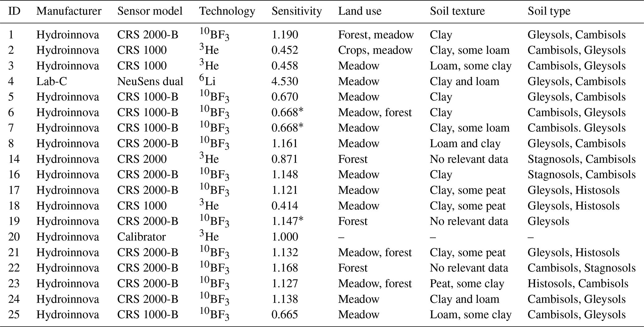
^* Calibrator was not available so the sensitivity was obtained from the average for other sensors of the same model.

3 Data

3.1 CRNS measurements

In total, 24 stationary CRNS detectors were positioned in the study area from May to July 2019. For various organizational and technical reasons, some sensors recorded only briefly or patchily. For the present analysis, we only used the 18 sensors that coherently covered at least the majority of the study period, including the manual sampling campaign at the end of June 2019. Table 1 gives an overview of those sensors and Fig. 1 shows their locations (see Fersch et al., 2020a for details about the different detector technologies used).

The placement of the CRNS sensors was performed under a set of scientific, legal, and practical constraints. Some of the constraints conflicted with each other (Fersch et al., 2020a); e.g. we aimed to maximize the spatial coverage of the catchment but also the overlap between sensor footprints. As a compromise, the CRNS sensors were placed more densely in the north-western part of the study area, where SoilNet observations were available for comparison (see Fig. 1).

The sensitivities of the detectors used in this study varied by over an order of magnitude between the most sensitive, NeuSense Dual, and the least sensitive, CRS-1000. However, the effective sensitivity could also differ between sensors of the same type. In order to standardize neutron count rates across sensors, we consecutively collocated a mobile “calibrator” sensor (#20 in Table 1) with most of the stationary probes for a duration of at least one day.

We used mobile CRNS measurements carried out from 25 to 26 June as another sensitivity reference. During those two days, a roving CRNS sensor (see Fersch et al., 2020a, for details) was placed next to the stationary CRNS sensors (except for sensors 1, 21, and 22, due to inaccessibility) for a duration of at least 30 min. The high sensitivity of the roving CRNS sensor meant that count rates from it were sufficiently representative that they could be related to the count rates of the stationary sensors.

3.2 Incoming cosmic-ray neutron flux and meteorological observations

In order to account for the variation in the incoming cosmic-ray neutron flux, Schrön et al. (2016) recommend the selection of recordings from neutron monitors that have similar cutoff rigidity to the study location. In this study, we used the monitor at Jungfraujoch to quantify the reference flux. The data were obtained from the Neutron Monitor Database (monitor ID “JUNG”, http://www.nmdb.eu, last access: 26 July 2021).

The location of the climate gauge at the Fendt site is shown in Fig. 1. The observed climate variables required for the present analysis included precipitation, barometric pressure, and the relative humidity and temperature of the air recorded at a temporal resolution of 1 min.

3.3 Local measurements of soil water content and other soil variables

Local measurements of soil water content and soil bulk density were required to calibrate the relationship between epithermal neutron intensity and volumetric soil water content. The same was true of the verification of soil moisture retrievals from observed neutron intensities. During the JFC, the following measurement techniques were applied to meet these requirements.

3.3.1 Permanent soil sensor network (SoilNet)

The north-west of the catchment is permanently equipped with a SoilNet (version 3, SoilNet, 2018), a network of 55 vertical sensor profiles (locations shown in Fig. 1). The temperature and permittivity are recorded at depths of 5, 20, and 50 cm at intervals of 15 min. Measurements are performed redundantly at each depth with two slightly displaced sensors. Please see Fersch et al. (2020a) for further details on how volumetric soil moisture was obtained from permittivity measurements.

3.3.2 Manual soil sampling and measurement of soil water content

Vertical measurements were carried out from 25 to 26 June 2019 at depth increments of 5 cm down to a maximum depth of 30 cm. A vertical profile was measured right beside each stationary CRNS sensor using soil cores and thermogravimetry. Vertical profiles using the same depths were obtained from manual FDR measurements at another 139 locations at and in-between the stationary CRNS sensors. Figure 1 provides an overview of the sampling locations. Please see Fersch et al. (2020a) for a comprehensive description of the sampling scheme, the sample processing for thermogravimetry, and the conversion of the measured permittivity to the volumetric water content for the FDR measurements.

3.4 Vegetation and biomass

For grassland and cropland, above-ground biomass was measured on three dates (14–16 May, 6 June, and 17 July) at the same 45 locations, and the water content was determined by drying to a constant weight at 65 ^∘C.

To quantify above-ground biomass in the forest, a different approach was used. Ground-truth information from 116 sites with a representative species composition allowed the derivation of a tree-species map using multitemporal RapidEye imagery. In addition, detailed tree-based surveys at 16 plots (including species, height, and diameter at breast height, see Fersch et al., 2020a for details) yielded above-ground biomass estimates. Using stand-height information from LIDAR, these estimates were generalized for the entire forested area (Stockmann, 2020).

4 Methods

4.1 Homogenization of neutron intensities over space and time

In order to make the observed neutron count rates comparable across space and time, different effects had to be taken into account, namely the different detector sensitivities, atmospheric effects, and the effects of hydrogen pools other than soil water.

4.1.1 Standardization of sensitivity

Measurements of a collocated calibrator probe (see Sect. 3.1) served to standardize the CRNS measurements. For the period of collocation, the ratio between the corresponding stationary and mobile neutron counts was defined as the sensitivity factor (constant over time, see Schrön et al., 2018a), which was then applied to standardize – to the calibrator level – the neutron intensities recorded by a stationary detector. When a calibrator collocation was missing, the average value from other sensors of the same model was used instead (see Table 1).

4.1.2 Accounting for atmospheric effects

The observed neutron count rates are affected by a range of dynamic atmospheric variables that need to be accounted for in order to make the neutron intensities comparable across time. These dynamic variables include the atmospheric vapour content, barometric pressure, and incoming cosmic-ray neutron flux. To correct for these effects, we used the data mentioned in Sect. 3.2. The corresponding standard correction approach is outlined by e.g. Scheiffele et al. (2020) (see Appendix A).

4.1.3 Accounting for the effects of vegetation

We assumed that the spatial variability of above-ground biomass is dominated by the presence of woodland in contrast to grassland: the average above-ground dry matter for grassland and cropland amounted to 0.2 kg m⁻², while the average above-ground dry mass for the forested area was quantified as 24.4 kg m⁻² (Stockmann, 2020). The spatial variability of forest biomass turned out to be high. However, its quantification at high spatial resolution (i.e. on the order of 100 m²) included considerable uncertainties. Therefore, we decided to use only the average above-ground biomass estimates for forest and grassland. The corresponding spatial distribution of above-ground biomass (in kg m⁻²) was represented on a regular grid with a horizontal resolution of 10 m. Based on this grid, we computed the weighted average above-ground dry matter per CRNS sensor footprint using the horizontal weighting function $W_{\mathrm{r}}/r$ as suggested by Schrön et al. (2017), and assumed these values to be constant throughout the duration of the campaign. On that basis, we accounted for the effect of vegetation on neutron count rates by following Baatz et al. (2015), who suggested a neutron intensity reduction of 0.9 % per kg of dry biomass per m².

4.1.4 Estimating average soil properties per sensor footprint

As pointed out in Sect. 3.3.2, the vertical distributions of volumetric water content (θ), soil bulk density (ρ_b), soil organic matter content (SOM), and lattice water content (LW) were determined at each CRNS sensor using thermogravimetry. For the volumetric water content, additional vertical profiles were measured using the FDR technique. Representative averages of these variables had to be obtained for each CRNS footprint in order to estimate N₀ (Sect. 4.2). For that purpose, we first approximated the three-dimensional distributions of soil properties from the available measurements and then applied the vertical and horizontal weighting functions provided by Schrön et al. (2017) in order to compute weighted averages. This involved the steps detailed below.

Fitting vertical profiles

In order to generalize the vertical distributions v_i of the soil variables (i.e. θ, ρ_b, SOM, LW) across the study area, we fitted a piecewise linear function to each profile and variable. From the soil surface (0 cm) down to a depth of 13 cm, the function assumed that each variable varied linearly from v_i(0 cm) to v_i(13 cm). Below 13 cm depth, the variable was assumed to remain constant at the value v_i(13 cm). This approach was found to reflect the typical vertical distributions of all soil variables fairly well while reducing spurious effects of outliers when the variables were horizontally interpolated (see the next section). Examples of profiles are illustrated in the Supplement (Figs. S1–S3).

Horizontally interpolating the vertical distribution parameters

The fitted parameters v_i(0 cm) and v_i(13 cm) at each profile location were then interpolated in space using ordinary Kriging with an exponential variogram model and a range of 50 m (150 m for soil moisture) on a 10×10 m grid (nugget and sill were set to 0 and 1, respectively). Based on the vertical distribution function and the interpolated parameters, we computed the value of each soil variable at 1 cm vertical resolution between 0 and 30 cm. It should be noted that, in this study, we applied ordinary Kriging heuristically rather than in a formal geostatistical way: stationarity was assumed and an exponential variogram model with a specific range was chosen in order to create continuous and plausible spatial patterns that are robust in areas of extrapolation and in which spatial autocorrelation was explicitly considered (instead of the implicit assumptions used in techniques such as nearest neighbour and inverse distance weighting). The sensitivity of our results to the range parameter was explicitly investigated in a Monte Carlo analysis (see Sect. 4.3).

The procedure was modified for soil organic matter and lattice water because these variables were not determined for each profile separately. Instead, these variables were determined for mixtures of samples obtained within areas classified as “forest on mineral soil”, “other land use on mineral soil”, or “other land use on organic soil” (see Fersch et al., 2020a). Hence, the vertical distribution function of each variable was determined for each of these three classes, and, instead of interpolation, the same vertical profile was assigned to each grid cell based on its membership of one of the three classes.

Computing the weighted average variable value for each sensor footprint

In the final step, we used the weighting functions from Eq. (A1) in Schrön et al. (2017) to compute average values of the soil variables per sensor footprint. The vertical average was obtained for each grid cell in the footprint based on the vertical weighting function W_d and the horizontal distance r of the grid cell from the sensor. Then the vertical averages were averaged horizontally based on the horizontal weighting function $W_{\mathrm{r}}/r$. As the soil variables of interest are parameters of the weighting functions themselves, the weighting procedure was iterated until the average variables converged (typically after less than five iterations), as recommended by Schrön et al. (2017).

4.2 Calibration of N₀

The soil water content was estimated from the epithermal neutron count rate using the standard transfer function suggested by Desilets et al. (2010). This required the calibration of the parameter N₀ based on local soil moisture observations.

$$\begin{array}{}\text{(1)}& {\mathit{\theta }}_{\mathrm{g}}^{\mathrm{all}}={\mathit{\theta }}_{\mathrm{g}}+{\mathit{\theta }}_{\mathrm{g}}^{\mathrm{som}}+{\mathit{\theta }}_{\mathrm{g}}^{\mathrm{lw}}={\displaystyle \frac{a_{\mathrm{0}}}{N/N_{\mathrm{0}}-a_{\mathrm{1}}}}-a_{\mathrm{2}},\mathit{\theta }={\displaystyle \frac{{\mathit{\varrho }}_{\mathrm{b}}}{{\mathit{\varrho }}_{\mathrm{w}}}}\cdot {\mathit{\theta }}_{\mathrm{g}}\end{array}$$

In Eq. (1), the subscript g indicates gravimetric soil water (equivalents) in units of kg kg⁻¹; hence, θ_g is the gravimetric soil water content, ${\mathit{\theta }}_{\mathrm{g}}^{\mathrm{som}}$ and ${\mathit{\theta }}_{\mathrm{g}}^{\mathrm{lw}}$ are the gravimetric soil water equivalents of soil organic matter and lattice water, θ is the volumetric soil water content (in m³ m⁻³), and ρ_w and ρ_b are the density of water (assumed to be 1000 kg m⁻³) and the soil bulk density (in kg m⁻³), respectively. N is the corrected neutron intensity (in counts per hour, cph) and N₀ (in cph) is the calibration parameter. The shape parameters a₀, a₁, and a₂ can be adapted to specific local conditions, but they have also proven robust in many previous studies (Desilets et al., 2010; Evans et al., 2016; Schrön et al., 2017, among others). They were set to a₀=0.0808, a₁=0.372, and a₂=0.115. Please note that water equivalents from vegetation (θ_bio) are not included in the sum on the left since the effects of vegetation biomass are already accounted for in the corrected neutron intensity N (see Sect. 4.1.3).

In order to use Eq. (1) to compute θ_g(N) or θ(N) from the observed neutron count rate N, θ^som and θ^lw as well as the soil bulk density ϱ_b need to be independently quantified as weighted averages for each CRNS sensor footprint (see Sect. 4.1.4 for details). For any calibration of N₀, θ needs to be independently quantified as a calibration reference that we refer to as θ^obs. ${\mathit{\theta }}_i^{\mathrm{obs}}$ was computed as a weighted average for each CRNS sensor footprint i from manual measurements (Sect. 4.1.4).

Usually, N₀ is calibrated for a single CRNS sensor at a particular site. For our dense cluster, however, we calibrated Eq. (1) by assuming a uniform value of N₀ across the study area. Hence, we optimized N₀ by minimizing the mean absolute difference between the average volumetric soil moisture ${\mathit{\theta }}_i^{\mathrm{obs}}$, and the corresponding θ(N_i,N₀), which can be obtained by solving Eq. (1) for θ and using the corrected neutron intensities N_i:

$$\begin{array}{}\text{(2)}& \underset{N_{\mathrm{0}}}{\arg \min }\sum _{i=\mathrm{1}}^{\mathrm{18}}\left|{\mathit{\theta }}_i^{\mathrm{obs}}-\mathit{\theta }\left(N_i,N_{\mathrm{0}}\right)\right|.\end{array}$$

The manual soil moisture measurements were carried out over two consecutive days, 25–26 June 2019 (see Sect. 3.3). Hence, the temporally varying parameters (the neutron count rates N_i, barometric pressure, and humidity) required as inputs for the weighting functions and Eq. (2) were obtained by computing temporal means between 08:00 UTC on 25 June and 18:00 UTC on 26 June.

4.3 Exploring the uncertainty of N₀ calibration

Uncertainties in the N₀ estimation arise from errors in the measurement of soil moisture and neutron fluxes as well as in the validity and parameterization of functional relationships and underlying assumptions. In order to get a better idea of both the robustness of our N₀ estimate and the uncertainty of the observed and CRNS-based soil moisture, we carried out a Monte Carlo analysis in which we repeated the N₀ calibration (see Eq. 2) 200 times, using a set of randomly disturbed input parameters each time (200 realizations were performed as they provided sufficiently robust results that did not change when more realizations were performed). The parameters and disturbances were as follows:

• Sensor sensitivity. As pointed out in Sect. 4.1.1, the neutron count rates of all sensors were standardized to the level of a calibrator. Yet, we still found some variability in the resulting sensitivity factors, even among sensors of the same type. In the Monte Carlo analysis, we assumed that the sensitivity varied by ±2 % with respect to the sensitivity level shown in Table 1.

• Averaging period for N_i. The definition of the time window for which the average neutron intensity N_i is calculated is rather arbitrary, particularly since the manual soil moisture measurements took place over a period of two consecutive days (from 08:00 UTC on 25 June to 18:00 UTC on 26 June). In order to capture the effect of the averaging period, we randomly selected 12 h windows within this time span and computed the average N_i from these windows.

• Dry vegetation matter. The spatial distribution of forest biomass is more relevant to the present study than that of grassland. Stockmann (2020) attempted to represent this distribution by combining allometric approaches with remote sensing and found that the dry matter mass varied between 13–73 kg m⁻², with a relative error of 17 % at the plot scale. As we used one uniform biomass estimate for the forest area (section 4.1.3), we expect large local errors. In our Monte Carlo analysis, we varied the dry matter mass per CRNS footprint within ±20 % of the estimated value.

• Water equivalent. As pointed out in Sect. 4.1.4, soil organic matter and lattice water contents were only determined from mixed samples for three different land-use/soil combinations. Hence, local values for the resulting water equivalents could substantially depart from these average values. We assumed that the estimated values of θ^som and θ^lw per footprint vary within ±20 % of the initial estimate.

• Kriging range. The choice to use an exponential variogram model together with a specific Kriging range for specific variables was made rather arbitrarily (Sect. 4.1.4). Hence, we varied the Kriging range values within ±50 % of the original values, resulting in a sampling interval of 75–225 m for soil moisture and 25–75 m for bulk density.

• Subsampling from soil profiles. For the N₀ calibration, the vertical soil moisture distribution was sampled at 160 locations in the study area. Given the size of the area and the number of CRNS sensors, the corresponding sample size per CRNS sensor was quite low compared to previous studies (18 samples per footprint were recommended by Zreda et al., 2012). In order to analyse how the availability of sampling locations affected the N₀ calibration, we employed a subsampling approach: for each Monte Carlo realization, we used only 80 % of our sampling locations for the interpolation of bulk density and volumetric soil moisture. These 80 % were randomly selected from the entire population of locations.

4.4 Soil moisture retrieval and spatial interpolation

To improve the signal-to-noise ratio for each CRNS sensor, we computed the average neutron count rate at intervals of 24 h and then, for each CRNS sensor, converted this averaged neutron count rate to the daily volumetric soil water content using Eq. (1) and the calibrated N₀. This soil water content will be referred to as θ(N_i) in the following. These values were examined as they were considered a first-order representation of how the soil water content varied in the study area over space and time.

In order to represent the spatial soil moisture distribution within and between CRNS footprints, we interpolated θ(N_i) to a 10 m × 10 m grid spanning the entire study area. The grid resolution was arbitrarily selected and does not necessarily reflect the resolution at which the grid effectively conveys information on the spatial heterogeneity; in other words, the product should not be interpreted at the scale of 10 m. Still, this comparatively fine horizontal resolution was needed since some of the subsequent steps required the re-aggregation (i.e. the averaging) of the spatial soil moisture estimates inside a CRNS footprint.

Gridded soil moisture estimates were obtained by two spatial interpolation approaches (models), which we will refer to here as the “unconstrained” and “constrained” models.

4.4.1 Unconstrained model

What we refer to as the unconstrained approach could imply any kind of model m that represents the spatial distribution of the soil moisture θ on the basis of parameter set p. This could be a geostatistical interpolation approach or, for instance, a distributed hydrological model.

In this study, for model m, we used ordinary Kriging with an exponential variogram model (nugget = 0, sill = 1) and a range parameter of, say, 300 m, using the CRNS sensor locations as data points for the interpolation. This choice was fairly arbitrary and subjective but reflects the spatial scale at which we are interested in representing the variation of soil moisture. With a given number n of CRNS sensors in our study area, the resulting model m(p) has n parameters, namely those of the n soil moisture θ_i at CRNS sensor location i (the data points for the interpolation), the values of which we set to the CRNS-based soil moisture estimates θ(N_i).

This interpolation approach has one major drawback: it does not account for the consistency between the obtained spatial soil moisture distribution (the output of m(p)) and the neutron intensities observed at the sensor locations (N_i) (and is hence “unconstrained”). If we were able to simulate the neutron intensities corresponding to the output of m(p), we would have a basis to constrain (or optimize) our parameters p by maximizing the agreement between the observed and simulated neutron intensities.

4.4.2 Constrained model

The constrained model m we used is the same as the above unconstrained model except that we adjust our initial guess of p such that the disagreement (here the sum of absolute differences) between the observed neutron count rates $N_i^{\mathrm{obs}}$ and the simulated count rates $N_i^{\mathrm{sim}}$ (obtained from m(p)) is minimized (Eq. 3):

$$\begin{array}{}\text{(3)}& \underset{\mathit{p}}{\arg \min }\sum _{i=\mathrm{1}}^n\left|N_i^{\mathrm{obs}}-N_i^{\mathrm{sim}}\left(m\right(\mathit{p}\left)\right)\right|.\end{array}$$

Figure 2a–f illustrates the idea and effects of a constrained model for a simple one-dimensional example with two CRNS sensors and an (unknown) true soil moisture distribution (solid black line, Fig. 2a). Figure 2b illustrates the sensor locations together with their horizontal sensitivity pattern (red shadows). Using a suitable forward operator  (Sect. 4.4.3), we can compute the neutron count rates $N_i^{\mathrm{obs}}$ that we would expect the sensors to observe based on the true soil moisture. These $N_i^{\mathrm{obs}}$ constitute the only information we have from our CRNS sensors. From these $N_i^{\mathrm{obs}}$, we compute the average soil moisture $\mathit{\theta }\left(N_i^{\mathrm{obs}}\right)$ based on Eq. (1) with a known N₀ (Fig. 2c). We then apply the unconstrained interpolation using $\mathit{\theta }\left(N_i^{\mathrm{obs}}\right)$ as data points (${\mathit{\theta }}_i^{\mathrm{node}}$, Fig. 2d). From the resulting soil moisture distribution (Fig. 2d, dashed line), we simulate the corresponding $N_i^{\mathrm{sim}}$, again using the forward operator . In the case of a marked soil moisture gradient, as in this example, the resulting $N_i^{\mathrm{sim}}$ and observed $N_i^{\mathrm{obs}}$ will disagree (Fig. 2e). The reason for this disagreement is obvious and unsurprising: if we use the volume-integrated $\mathit{\theta }\left(N_i^{\mathrm{obs}}\right)$ as a data point for the interpolation (${\mathit{\theta }}_i^{\mathrm{node}}$), we potentially neglect a substantial portion of spatial variation that is hidden behind this volume average. Hence, spatial gradients will tend to be systematically underrepresented: here, the unconstrained model underestimates areas of high soil moisture in the left half of our spatial domain and overestimates them in the right half.

Figure 2 Schematic view of the constrained interpolation model, illustrated by an idealized example with two CRNS sensors and a 1-D horizontal soil moisture distribution. Symbols are explained in the main text; note that the spatial domain extends further to the right but is not shown in full for the sake of clarity.

In the constrained model, we therefore adjust the values for ${\mathit{\theta }}_i^{\mathrm{node}}$ so that the disagreement between $N_i^{\mathrm{sim}}$ and the measured $N_i^{\mathrm{obs}}$ is minimized (Fig. 2f). This optimization problem could have an infinite number of equally valid solutions. The problem of equifinality is addressed, however, by using a local optimization technique (the Nelder–Mead simplex adapted according to Gao and Han, 2012). As our initial parameter guess for (${\mathit{\theta }}_i^{\mathrm{node}}$) is based on $\mathit{\theta }\left(N_i^{\mathrm{obs}}\right)$, we expect the parameter optimization to stay close to this initial guess, changing by only as much as required to better represent the local soil moisture gradients. We also expect that the optimization problem will be constrained better in areas where multiple CRNS sensors significantly overlap. Conversely, the difference between the initial $N_i^{\mathrm{sim}}$ and $N_i^{\mathrm{obs}}$ will probably be small for CRNS sensor locations that are rather isolated and distant from others. This is because the interpolated soil moisture values in the footprint of any isolated (or distant) sensor i will be dominated by $\mathit{\theta }\left(N_i^{\mathrm{obs}}\right)$ and less affected by other sensors.

4.4.3 The forward operator

The constrained model resembles what is generally referred to as geophysical inversion, i.e. the identification of parameters p in a model m by means of inverse simulation: the observed variable (N) is obtained from the estimated target variable (θ) by means of a physically based forward operator (i.e. simulation). Hence, p is optimized by minimizing the disagreement between simulation and observation. This allows further spatial information to be obtained from volume-integrated observations using our physical understanding of both the observed system and the observation technique itself. On this basis, our constrained approach, as outlined above, does not entirely qualify as a geophysical inversion for two reasons. First, we use a geostatistical instead of a physical model to describe our notion of soil moisture variation at a specific scale. Second, we use a rather heuristic implementation of the forward operator , which is specified as follows:

$$\begin{array}{}\text{(4)}& \textcolor{red}{}:{\mathrm{\Theta }}_i^{\mathrm{m}}\mapsto N_i^{\mathrm{sim}},\end{array}$$

where the operator  simulates the corrected epithermal neutron intensity $N_i^{\mathrm{sim}}$ at a sensor location i using the entire environment of interpolated (modelled) soil moisture values ${\mathrm{\Theta }}_i^{\mathrm{m}}$ in a 300 m radius around the sensor, leading to a grid in which each grid cell j has a modelled soil moisture value ${\mathit{\theta }}_j^{\mathrm{m}}$.

Shuttleworth et al. (2013) developed the COSMIC operator in the context of data assimilation. However, the COSMIC operator accounts for only the vertical – not the horizontal – variability of the soil moisture, and is therefore not eligible for our purpose. Neutron transport models, in turn, are able to track the histories of millions of neutrons by taking the relevant physical interactions into account, including not only the effects of soil moisture but also those of e.g. the vegetation or topography. Neutron transport models are available and have proven valid in a wide range of application contexts. Examples are MCNP (Andreasen et al., 2017) or, more recently, URANOS (Weimar et al., 2020). Both would be suitable forward operators for our application except that their computational cost would be prohibitive: the optimization of p requires hundreds of iterations – requiring weeks of computation time – for soil moisture interpolation at just one point in time.

Hence, in this work, we followed an intermediate approach that we have already referred to as heuristic. In our approach, instead of explicitly simulating the physical interactions of neutrons with the near-surface environment, we use the horizontal weighting function W_r presented in Eq. (A1) of Schrön et al. (2017). W_r represents the horizontal sensitivity pattern of a CRNS sensor, which depends on various somewhat dynamic environmental variables such as the soil moisture itself, soil bulk density, vegetation, air humidity, and barometric pressure. Though W_r was not originally intended to support forward simulation, it is obtained via extensive neutron transport simulations (Köhli et al., 2015) and therefore has a sufficient physical basis to serve our main purpose: to quantify, based on the observed neutron intensity at a particular location i, the relative contributions of soil moisture at different distances from the sensor. W_r does not, however, directly yield the neutron intensity (formally, we use it as a spatial filter). Hence, we combine W_r with the inverse of Eq. (1) to obtain the forward operator presented in Eqs. (5) and (6) below:

$$\begin{array}{}\text{(5)}& {\displaystyle }& {\displaystyle }{N}_i^{\mathrm{sim}}=\textcolor{red}{}\left({\mathrm{\Theta }}_i^{\mathrm{m}}\right)=N_{\mathrm{0}}\cdot {\displaystyle }+a_{\mathrm{1}}\text{(6)}& {\displaystyle }& {\displaystyle }〈{\mathrm{\Theta }}_i^{\mathrm{m}}〉={\displaystyle \frac{\sum _j\left(W_{\mathrm{r},i,j}\cdot {\mathit{\theta }}_j^{\mathrm{m}}\right)}{\sum _j{W}_{\mathrm{r},i,j}}}+{\mathit{\theta }}_i^{\mathrm{lw}}+{\mathit{\theta }}_i^{\mathrm{som}}.\end{array}$$

4.5 Comparison to the local soil sensor network (SoilNet)

In order to evaluate the performance of the unconstrained and constrained interpolation models, the resulting maps of average daily soil moisture were compared with daily soil moisture maps obtained from the FDR cluster (SoilNet) operated at the site (Fersch et al., 2020a). This comparison, however, was not straightforward: while the SoilNet data consist of a set of observations at specific points in space (with a horizontal support of a few centimetres), the results of the interpolation models are spatial soil moisture grids with varying degrees of vertical representativeness.

The SoilNet observations ${\mathit{\theta }}_{\mathrm{n},z}^{\mathrm{FDR}}$ constitute 55 nodes (index n), each of which provides measurements at three depths z (5, 20, and 50 cm; two measurements at each depth are averaged). For each node, we first obtained a continuous vertical profile: we linearly interpolated the measurements at intervals of 1 cm between 5 and 20 cm and between 20 and 50 cm. Between 5  cm and the soil surface, the value from 5 cm was used. To account for the CRNS penetration depth, we then computed a weighted vertical average $\langle {\mathit{\theta }}_n^{\mathrm{FDR}}\rangle$ at each node using the weighting function W_d from Schrön et al. (2017) (note that W_d depends on the distance r to a CRNS sensor, which is not unique when multiple CRNS sensors are present; in this work, we used a medium value of r=20 m for all SoilNet nodes since the penetration depth decreases by less than 5 cm within a distance of 100 m from a CRNS sensor for average soil moisture values of around 0.4 m³ m⁻³; see Fig. 8 in Köhli et al., 2015). Finally, we horizontally interpolated $\langle {\mathit{\theta }}_{\mathrm{n}}^{\mathrm{FDR}}\rangle$ to the same grid as the interpolated CRNS-based soil moisture using the same ordinary Kriging approach as used for the interpolation of CRNS-based soil moisture (exponential variogram with a range of 300 m).

We evaluated the similarity of the spatial soil moisture patterns obtained from the FDR cluster and the interpolation of θ(N_i) for each day from 20 May to 15 July 2019. We chose Spearman's rank correlation of the corresponding soil moisture grids as a measure of similarity. Using that measure, we eliminated potential effects of uncertainty in the soil moisture values obtained from the SoilNet, as the conversion from permittivity to volumetric soil moisture can be subject to systematic bias (Mohamed and Paleologos, 2018).

5 Results and discussion

5.1 Can we find a uniform N₀ for the entire study area?

The parameter N₀ in Eq. (1) accounts for a variety of factors in the relationship between soil moisture and neutron intensity (e.g. sensor sensitivity and hydrogen pools other than soil water). N₀ should be the same for each sensor if the observed neutron intensities are perfectly homogenized with regard to these effects, and if the calibration reference is error-free. Based on our homogenization efforts (Sect. 4.1 and the successful standardization of sensitivity, as documented in Sect. S2), we estimated an N₀ value of 3723 cph with a mean absolute error of 0.047 m³ m⁻³ for θ (see Table 2 for an overview of the calibration input and output). Figure 3a contrasts CRNS-based soil moisture estimates θ(N) with the calibration reference θ^obs. Figure 3b illustrates how well the relation between gravimetric soil water content ${\mathit{\theta }}_{\mathrm{g}}^{\mathrm{all}}$ and neutron intensity N corresponds to Eq. (1).

Figure 3 Results of the N₀ calibration: (a) shows the θ(N_i) obtained from standardized and corrected neutron count rates N_i versus the conventional soil moisture estimates ${\mathit{\theta }}_i^{\mathrm{obs}}$, i.e. footprint-averaged volumetric soil moisture obtained from manual sampling (25–26 June 2019). The grey shadows indicate deviations of 2.5 % and 5 % in θ(N_i). The bottom panel provides a different perspective by plotting N_i versus the observed total gravimetric soil water content, including water equivalents from soil organic matter and lattice water; the dashed line indicates the Desilets function, Eq. (1), with a calibrated N₀=3723 cph.

While the agreement is not perfect, the general pattern suggests that CRNS-based soil moisture estimates obtained from a single N₀ can explain a substantial portion of the variability in the study area (R²=0.69), where soil moisture ranges from 0.33 to 0.70 m³ m⁻³. Yet, some sensors display remarkable disagreement between ${\mathit{\theta }}_i^{\mathrm{obs}}$ and θ(N_i); this is most notable for sensor 7 (−0.15 m³ m⁻³), but is also seen for sensor 22 (+0.09 m³ m⁻³), sensor 5 (+0.08 m³ m⁻³), and sensor 23 (−0.07 m³ m⁻³).

We would like to put these disagreements into perspective by providing a better idea of the uncertainties involved in the N₀ calibration on 25–26 June. Based on the Monte Carlo analysis (Sect. 4.3), Fig. 4 displays the local uncertainty of θ(N_i) and ${\mathit{\theta }}_i^{\mathrm{obs}}$ (Fig. 4a) as well as the local uncertainty in N_i and ${\mathit{\theta }}_{\mathrm{g},i}^{\mathrm{all}}$ (Fig. 4b). Here, the term “local” refers to the uncertainty for a specific sensor footprint i (please see the figure caption for details).

Figure 4 Results of the Monte Carlo analysis: (a) shows θ(N_i) versus ${\mathit{\theta }}_i^{\mathrm{obs}}$, while (b) shows the corrected neutron intensities N_i over the gravimetric soil water equivalent ${\mathit{\theta }}_{\mathrm{g},\mathrm{i}}^{\mathrm{all}}$. The dark grey shaded areas represent the interquartile ranges of these variables based on the 200 realizations in the Monte Carlo analysis. The horizontal and vertical extents of the dark grey shaded areas are used to measure the local uncertainties in these variables, where the term “local” refers to the uncertainty for a specific sensor footprint i. The light grey shaded areas in (a) show the inner 90 % of the realizations for illustrative purposes only. (c) shows the distribution of all 200 N₀ values, highlighting the interquartile range in dark red and the inner 90 % in light red. Accordingly, the dark and light red shaded areas in (b) indicate the range of the Desilets function when using the interquartile range and the inner 90 % of N₀ realizations, respectively.

The results shown in Fig. 4 can be seen as both unfavourable and encouraging. The level of local uncertainty expressed by the vertical and horizontal extents of the dark grey shaded areas is rather unfavourable. The uncertainty of θ(N_i) is a location-specific combination of uncertainties, e.g. of the above-ground forest biomass, the mean N_i (which was represented by temporal subsampling), and the spatial distribution of the soil bulk density. The average uncertainty of θ(N_i) (i.e. the mean width of the dark grey boxes along the y axis) amounts to 0.08 m³ m⁻³. However, there is also some uncertainty in θ_obs (the so-called ground truth): 0.03 m³ m⁻³ on average for the dark grey boxes along the x axis. This uncertainty mainly results from the limited spatial density of the measured profiles.

It is encouraging, though, that the estimation of N₀ appears quite robust, and that there is no evidence to suggest that N₀ is sensor dependent (except for sensor 7). The 25th and 75th percentiles of N₀ amount to 3677 and 3733 cph, respectively, which correspond to a range of less than 1.5 % relative to the optimal value of N₀=3723 cph (Fig. 4c). The dark grey boxes that represent the interquartile ranges of θ(N_i), ${\mathit{\theta }}_i^{\mathrm{obs}}$, and N_i clearly overlap with the diagonal (Fig. 4a) and (in most cases) with the curve of the Desilets function (Fig. 4b).

The only box that overlaps with neither the diagonal nor the Desilet function is that for CRNS sensor 7. We therefore cannot assume that the N₀ value of 3723 cph is valid for this CRNS location. Currently, we do not have a satisfactory explanation for this: the uncertainties of the vegetation biomass, soil organic matter, and lattice water around sensor 7 cannot explain this level of disagreement, and it appears that the sensitivity was successfully standardized for sensor 7 (the neutron intensity from sensor 7 corresponds well to the rover measurement; see Fig. S4). It is possible, though, that the reference soil moisture ${\mathit{\theta }}_{\mathrm{7}}^{\mathrm{obs}}$ is too high: the soils appear to become drier towards the west, and a preliminary analysis of roving data from June 2019 indicates relatively dry conditions along the road south-west of sensor 7 (see Fig. 10 in Fersch et al., 2020a). At the same time, manual measurements were scarce in the western footprint of sensor 7 (due to access restrictions and technical issues that led to the loss of manual FDR profiles at five locations), so our estimate ${\mathit{\theta }}_{\mathrm{7}}^{\mathrm{obs}}$ might not be representative of the footprint. Still, we do not have hard evidence to support this hypothesis, so we decided to exclude sensor 7 from further analysis in the present study.

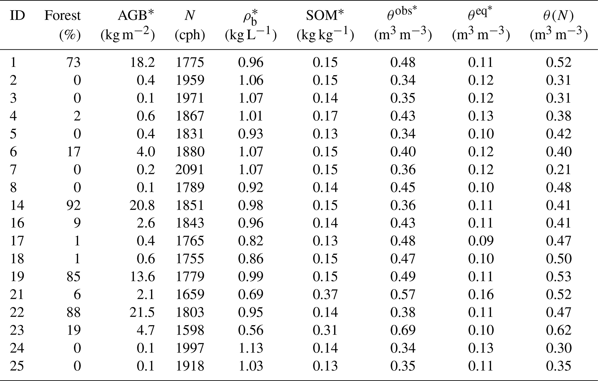
Table 2 Overview of calibration data and results per sensor (variables with an asterisk (^*) were computed as a weighted average per footprint). ID: sensor ID; Forest: percentage of forest area in the footprint; AGB: above-ground dry matter biomass; N: corrected neutron count rate averaged over the calibration period; ρ_b: soil bulk density (note that vertical weighting gives more weight to the top soil, where the bulk density tends to be lower; cf. Sect. 4.1.4 and Fig. S2); SOM: soil organic matter content; θ^obs: volumetric soil water content from manual measurements; θ^eq: volumetric soil water equivalent (θ^som+θ^lw); θ(N): volumetric soil water content as estimated from Eq. (1).

5.2 Spatial and temporal patterns in CRNS-based soil moisture

We used the joint N₀ value together with a 12 h moving average of the corrected neutron intensities and Eq. (1) to retrieve time series of volumetric soil moisture for the remaining 17 locations over the entire study period (Fig. 5).

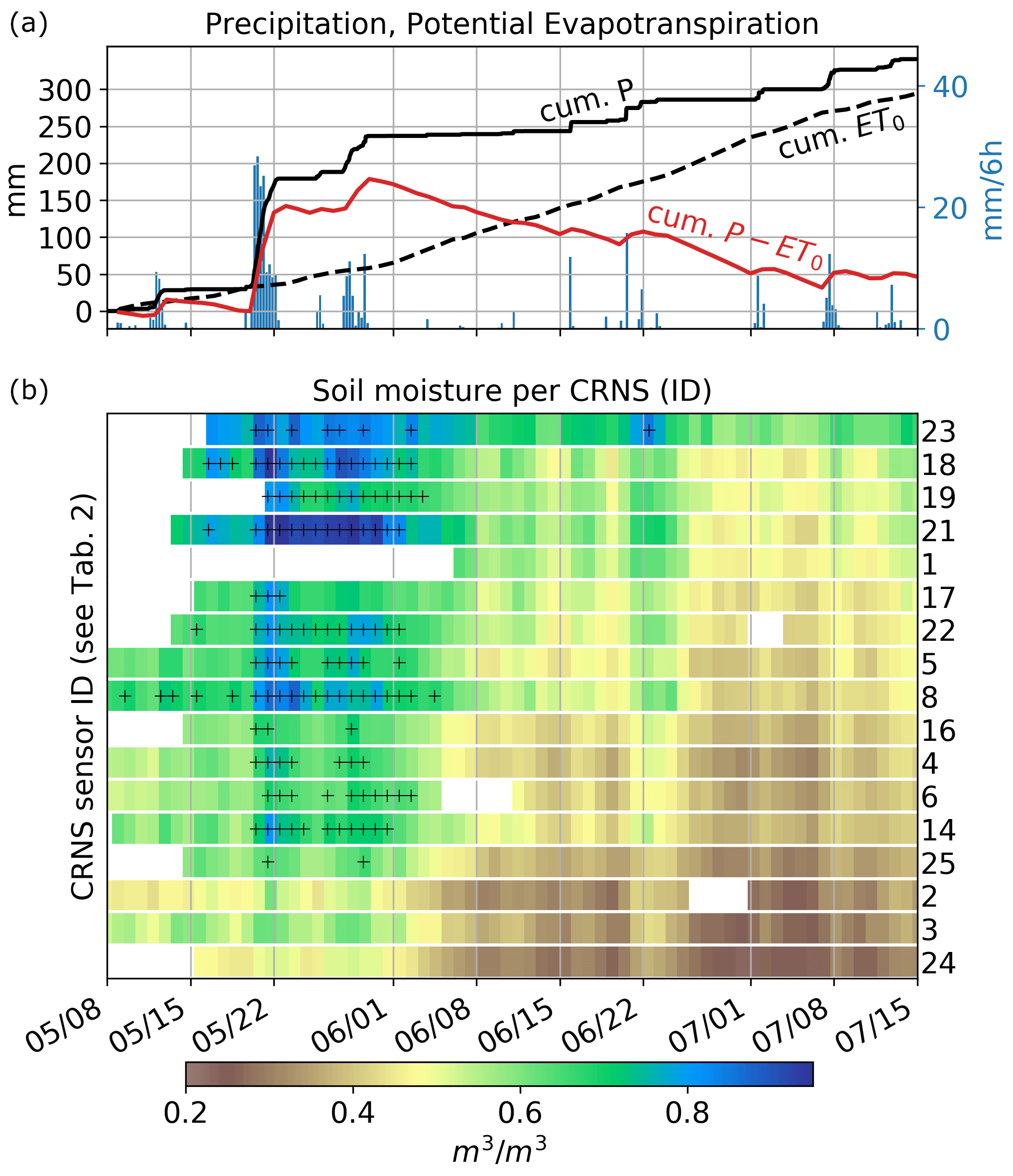
Figure 5 Time series of precipitation, reference evapotranspiration, and estimated soil water content. (a) Cumulative values of precipitation P (mm), reference evapotranspiration ET₀ (based on FAO, 1998, in mm), and the difference P− ET₀ (in mm); the precipitation depth (mm) obtained at 6 h intervals is shown as blue bars. (b) Soil moisture θ(N_i) as estimated for each CRNS sensor i; rows are arranged from top to bottom in order of decreasing average soil water content during the last week of the campaign (8–15 July). A white space indicates a period of missing data; black + signs indicate periods in which the apparent volumetric soil moisture exceeded the soil porosity, probably due to ponding.

Overall, we see strong temporal dynamics of wetting, drying, and re-wetting that correspond well to the cumulative difference between precipitation and reference evapotranspiration (the red line in the top panel of Fig. 5). Torrential rains of about 150 mm during 20–22 May marked the start of the campaign, with another 50 mm of rain observed until 29 May. During that period, the volumetric soil moisture exceeded the soil porosity in many locations (marked by the black + signs). This is in line with the observation that large parts of the study area were affected by ponding in the last week of May. The following drying period until 15 July was repeatedly interrupted by rainfall events of more than 10 mm (e.g. on 15 and 20 June and on 1, 7, and 12 July). Still, June marks the transition from saturated to moderately dry conditions: from 1 to 30 June, soil moisture dropped by 0.2–0.3 m³ m⁻³ at each CRNS sensor location (a decrease of between 25 % to 50 % relative to the soil moisture on 1 June).

The rows in the bottom panel of Fig. 5 are arranged from top to bottom in order of decreasing average soil water content during the last week of the campaign (8–15 July). Some spatial and temporal patterns emerge with this arrangement. Location 23, located in a large patch of peat soil, stands out due to its very high soil moisture (permanently above 0.5 m³ m⁻³ and with an average of 0.71 m³ m⁻³). At the other end, there are a group of relatively dry locations in the western parts of the study area (locations 2, 3, 4, 24, and 25) and a group of less (but still rather) dry locations along the eastern slopes towards the water divide of the catchment (locations 6, 14, and 16). In between, we find a series of locations with intermediate soil moisture levels and pronounced wetting and drying dynamics over the study period, most of them strung along the bottom of the central valley of the Rottgraben (locations 1, 5, 17, 18, and 21) as well as a drainage line from the eastern slopes (location 19). Location 8 is more peculiar: it is very close to the driest locations, starts off very wet, but also exhibits pronounced drying dynamics.

We have to keep in mind the results from Sect. 5.1, which indicated that there is large local uncertainty in θ(N). Hence, any ranking that is based on average soil moisture values should be interpreted with care. Take location 22 for instance: Fig. 3 suggests that θ(N) is probably overestimating soil moisture in this location, which is supported by the uncertainty range shown in Fig. 4. The dominant source of uncertainty at location 22 is most likely the above-ground forest biomass in the near range of sensor 22. Hence, location 22 could be around 0.1 m³ m⁻³ drier than shown in Fig. 5. However, the change in the rank of a CRNS sensor location over time (i.e. relative to other locations) should be less affected by such local (but presumably static) uncertainties. From a hydrological perspective, it might be informative to examine such changes in rank, as they may indicate changes in governing hydrological processes. As an example, location 21 was by far the wettest location in the last week of May, but only the fourth wettest location in the last week of the campaign. Similar to location 23, location 21 is characterized by peaty soils with low bulk density and high soil moisture, but it dries much faster. We hypothesize that during the heavy rainfall in May, location 21 collected near-surface interflow from the nearby eastern hillslopes, which, in combination with a local impermeable layer below the peat soils, led to a local accumulation of water. However, location 21 might not be influenced by the shallow aquifer as much as location 23, so it dries faster. While this hypothesis remains as-yet untested, it illustrates how a dense network of CRNS sensors in a heterogeneous landscape could help us to identify governing hydrological processes.

5.3 How does soil moisture vary within and between the sensor footprints?

5.3.1 Spatial interpolation of CRNS-based soil moisture

In this study, we aimed to use CRNS data to coherently and continuously represent the catchment-scale variation of soil water content at a resolution of tens to hundreds of metres, i.e. the variation within and between CRNS footprints. To obtain daily soil moisture maps, we applied two interpolation models (Sect. 4.4) – unconstrained and constrained models – to each day of the campaign. Figure 6 shows examples of maps for three different dates: 1 June (2 days after the continued rainfall in May 2019 ended), with very wet conditions; 7 June (after a week of drainage and evapotranspiration), with intermediate wetness; and 30 June (after another 3 weeks of drying), with relatively dry conditions.

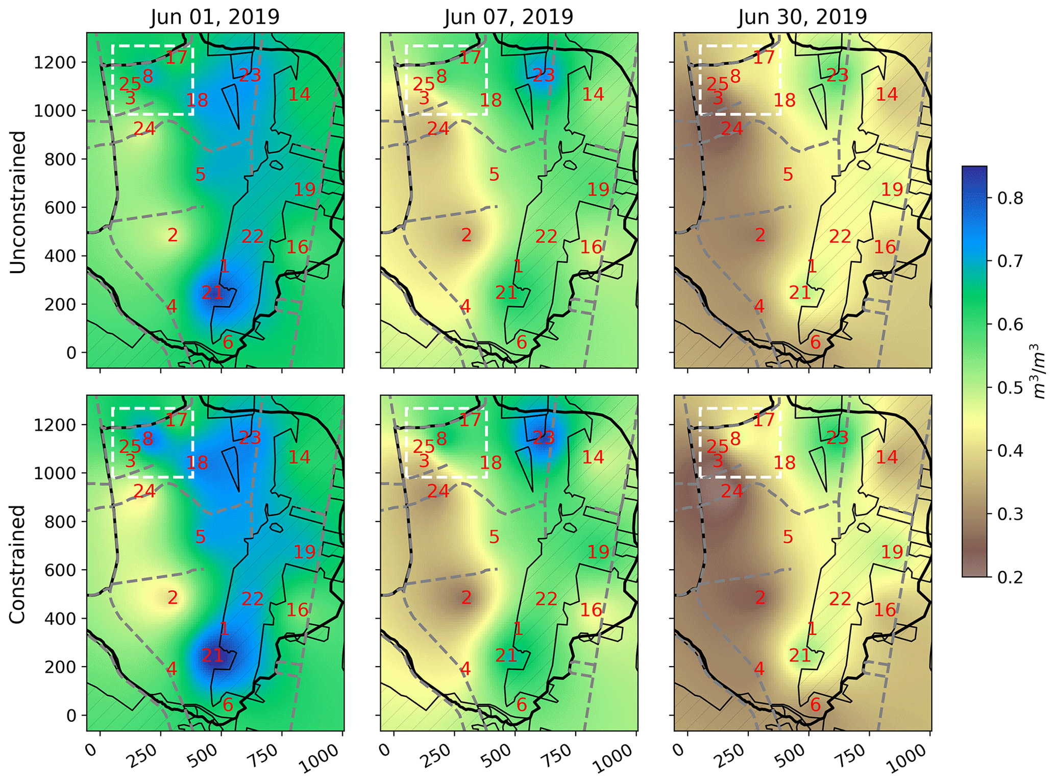
Figure 6 Daily average soil moisture on three different dates (left: 1 June, centre: 7 June, right: 30 June 2019) and for the unconstrained/constrained interpolation model (top/bottom row). Also shown are locations and IDs of the CRNS sensors used for the interpolation (red), the catchment boundary (black line), forest (grey hatching with a black contour), roads (dashed grey line), and the extent of the SoilNet (dashed white rectangle). The figure uses OSM basemap layers for land use and roads (© OpenStreetMap contributors 2020; distributed under the Open Data Commons Open Database License (ODbL) v1.0). (OpenStreetMap contributors, 2020).

The maps obtained using both interpolation models illustrate more intuitively what we learned in the previous section (Sect. 5.2): that the soils become considerably drier from the valley bottom of the Rottgraben towards the western parts and (to a less pronounced but still obvious degree) towards the eastern hillslopes. Furthermore, the locations of sensors 19 (at a drainage line) and 8 (in the SoilNet area) are rather wet. The maps also illustrate well how the drying of soils progresses spatially during June. At the same time, Fig. 6 demonstrates the differences between the two interpolation models: as expected, the constrained model enhances horizontal soil moisture gradients (leading to increased contrasts in the bottom panel maps).

The interpolation also allows us to compute a catchment-wide soil moisture average or to capture the frequency distribution of soil moisture values in the catchment at any point in time. Figure 7, for instance, shows the median as well as the inner 50 % and 90 % of the catchment-wide soil moisture values for both interpolation models. While the median values are almost identical, the models clearly differ at the tails of the distribution (most clearly for the 5th and 95th percentiles). This behaviour is consistent with the expectation that constrained interpolation enhances gradients.

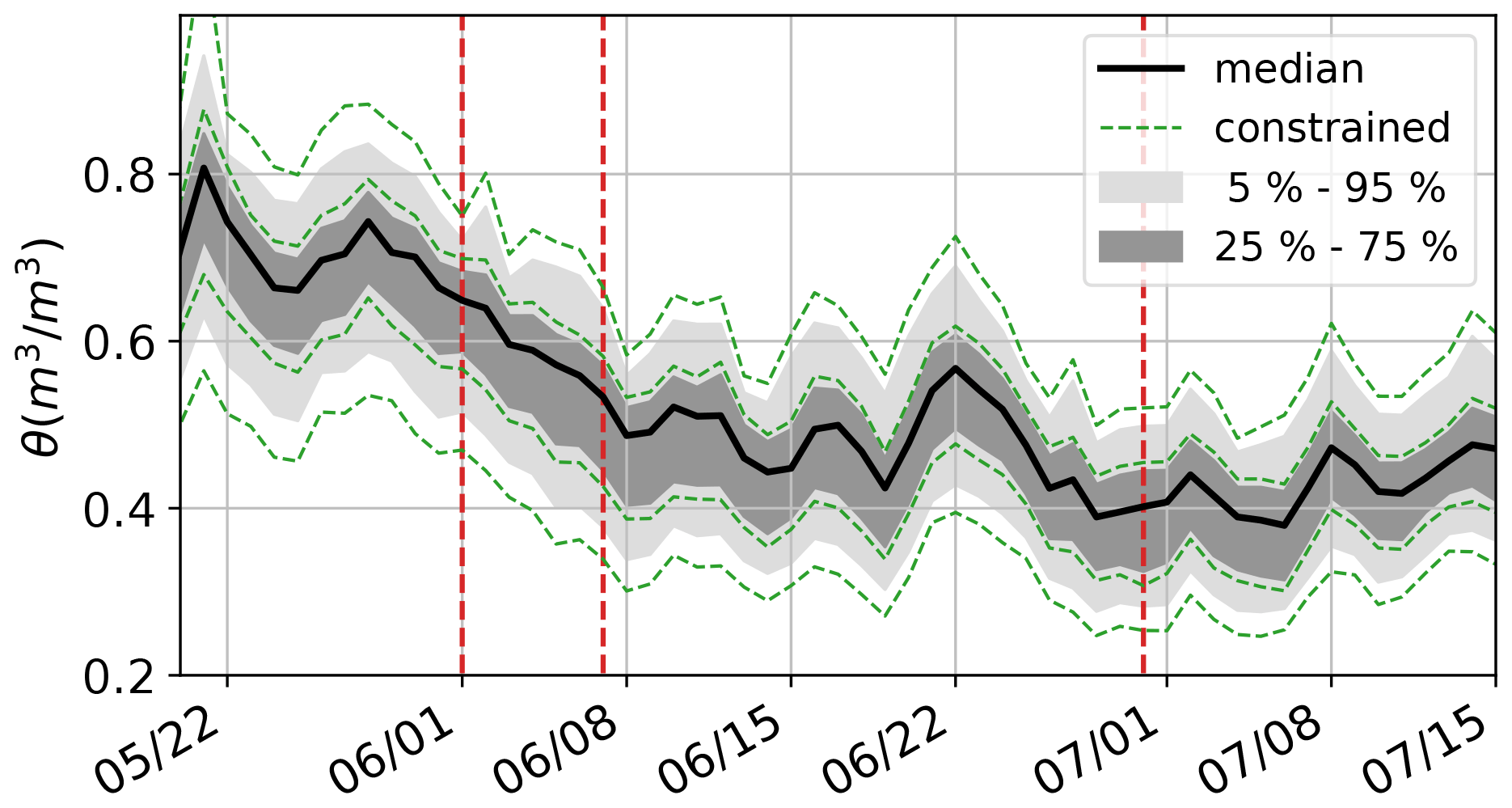
Figure 7 Catchment-wide median (black line), interquartile range (dark shadow), and inner 90 % (light shadow) of daily soil moisture values obtained from unconstrained interpolation. The dashed green lines indicate the corresponding percentiles (5th, 25th, 75th, and 95th) obtained from constrained interpolation ”(the median of the constrained interpolation is not shown in addition as it is almost identical to the unconstrained interpolation); the dashed red lines show dates used in Fig. 6.

5.3.2 Comparison of spatial patterns against SoilNet observations

The area of the SoilNet is particularly suited to a comparison of the interpolation models regarding their ability to represent soil moisture gradients. First, the SoilNet allows spatial variability to be captured due to its high sampling density. Second, the density of CRNS sensors is also higher in that area: the 150 m radii of six sensors (3, 8, 17, 18, 24, 25) substantially overlap with the SoilNet area. Third, the spatial heterogeneity of soil moisture in the SoilNet area appears quite pronounced (generally drier towards the west, with a wet anomaly at the centre).

For the comparison, we horizontally interpolated the vertically averaged FDR measurements to the same grid as used before (Sect. 4.5), and used only those parts of the grid that fell inside the spatial bounding box of the SoilNet. Figure 8 shows an example for 7 June 2019 (when there was intermediate wetness): the SoilNet shows a wet area in its central part that tends to extend to the north and the north-east as well as a pronounced progression towards drier conditions in the south-west and east. The soil moisture gradient from the centre to the south-west is fairly well captured by the constrained interpolation model, particularly in comparison to the unconstrained model; both models fail to reproduce the dry region at the eastern edge.

Figure 8 Daily average soil moisture in the SoilNet area on 7 June 2019, as obtained from the unconstrained interpolation (left panel), the constrained interpolation (centre panel), and the interpolated SoilNet measurements (right panel). The spatial window corresponds to the dashed white box in Fig. 6. Black circles: locations of the SoilNet nodes; red numbers: CRNS sensor locations and IDs.

In order to formalize the comparison, Fig. 9a shows the Spearman's rank correlation between the daily spatial soil moisture patterns. Apparently, the constrained model is superior (i.e. more similar to the SoilNet) for the majority of the study period, namely all of June. Only during the very wet beginning of the campaign (until early June) does the unconstrained model seem to outperform the constrained one. That period, however, has to be interpreted with care, since it was governed by substantial ponding, which obviously cannot be captured by the SoilNet sensors but can be detected by the CRNS network. We can also observe a general decline in the correlation between the CRNS-based interpolation products and the SoilNet towards the (drier) end of the campaign: in July, the differences in rank correlation between both interpolation models are rather negligible. Rainfall events tend to reduce the correlation, which is a well-known issue when using subsurface sensors as a reference: until rainfall infiltration advances to the upper SoilNet sensor (at 5 cm depth), the SoilNet does not register the event, while the CRNS sensors immediately react to the additional water at the soil surface – especially when it is close to the surface (Schrön et al., 2017; Scheiffele et al., 2020).

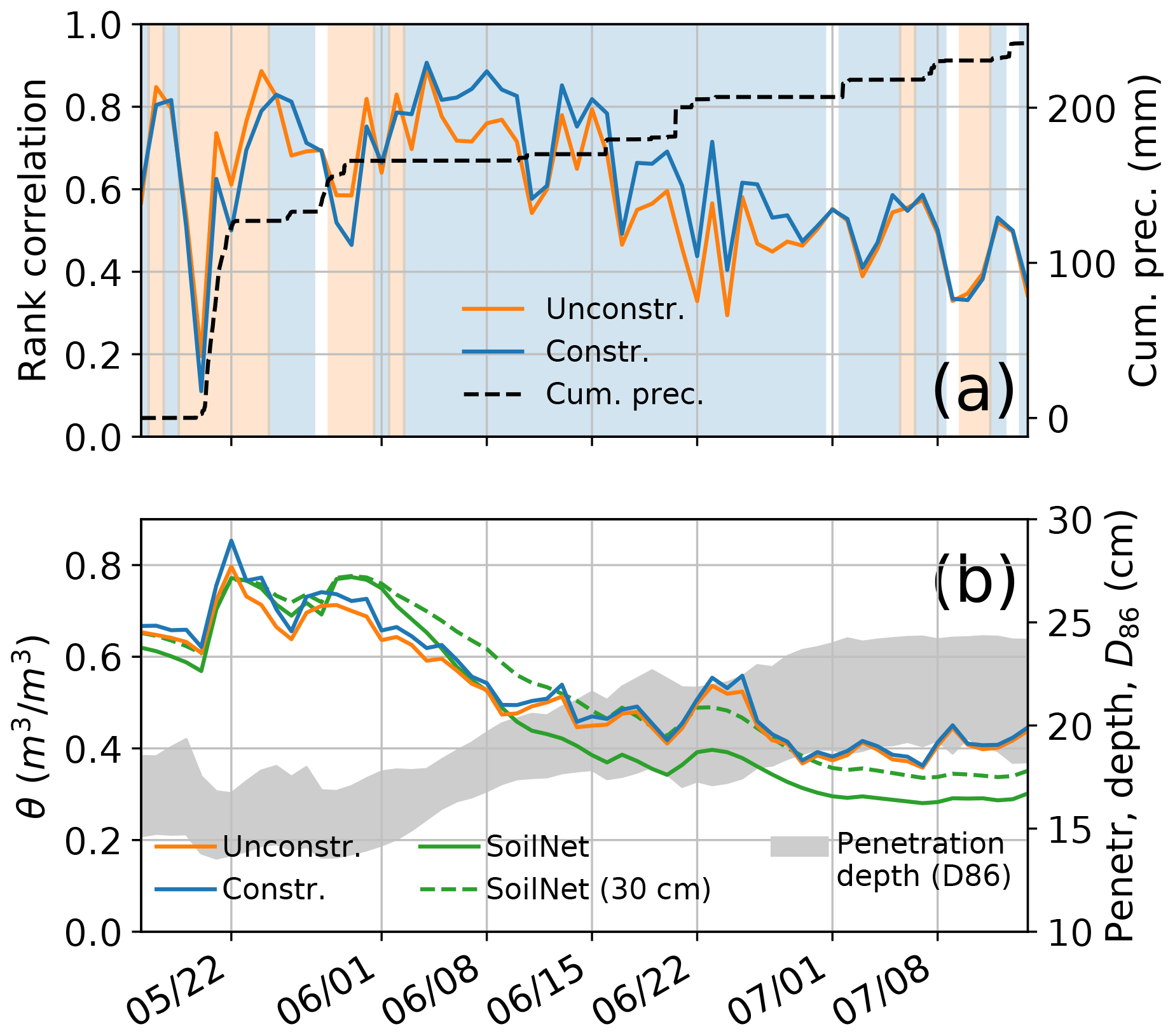
Figure 9 (a) The orange (blue) line shows the rank correlation between the daily average soil moisture pattern of the SoilNet and the pattern from the unconstrained (constrained) interpolation of θ(N); blue/orange backgrounds highlight days on which one model outperforms the other; the dashed black line shows the cumulative precipitation. (b) Average daily soil moisture across the SoilNet area as obtained from unconstrained/constrained interpolation (orange/blue), the vertically weighted SoilNet observations (solid green), and an unweighted vertical average of the upper 30 cm (dashed green); the grey shading represents the range of penetration depths (D86, the depth within which 86 % of neutrons probed the soil) in the footprints from the six CRNS sensors closest to the SoilNet area (CRNS 3, 8, 17, 18, 24, 25).

With regard to the spatial average of daily soil moisture across the SoilNet area (Fig. 9b), the differences between the two interpolation models are rather negligible, particularly in comparison to their disagreement with the SoilNet. That fact alone is unsurprising: compared to the unconstrained model, the constrained model enhances spatial gradients but it should not systematically affect the spatial average (Sect. 5.3.1). But what causes the disagreement between the SoilNet average 〈θ^FDR〉 and the CRNS-based averages 〈θ(N)〉, a disagreement that increases during June? So far, the reasons remain unclear, but we would like to mention three uncertainties. First, the SoilNet measurements at 5, 20, and 50 cm only allow for imprecise characterization of the vertical soil moisture profile, specifically in the dynamic upper 20 cm that affect the CRNS signal the most. Second, any bias in the conversion from permittivity to volumetric soil moisture might not be homogeneous across the observed range of soil moisture or soil properties in the SoilNet area (Sect. 4.5). Third, the weighting functions that were used to compute the vertical average ${\mathit{\theta }}_n^{\mathrm{FDR}}$ are not necessarily transferable to situations of pronounced horizontal and vertical heterogeneity (Köhli et al., 2015), and hence a known source of substantial uncertainty (Baroni et al., 2018). For illustrative purposes, Fig. 9b shows the range of computed penetration depths (D86) for six nearby CRNS sensors; D86 varies from 14–19 cm in May to about 19–24 cm in July. However, if we average θ^FDR uniformly over the upper 30 cm (dashed green line), the agreement with the CRNS-based averages appears to be somewhat better. The reasons for this behaviour remain unclear, but it emphasizes the possible uncertainty regarding the vertical representativeness of both the CRNS and the SoilNet observations.

So, while we have provided evidence that the constrained interpolation model captures horizontal soil moisture gradients better than the unconstrained model, the usefulness of the SoilNet observations in Fendt as reference data appears to be limited by a range of uncertainties. Future studies might address this issue by exploring other reference data for such benchmark experiences, e.g. roving transects such as those published by Fersch et al. (2020a).

6 Summary and conclusions

This study is the first attempt to analyse the observations of a dense CRNS network in a catchment of 1 km². Using a comprehensive homogenization process, we demonstrated the possibility of retrieving soil moisture using a joint N₀ value, capturing characteristic spatio-temporal features of soil moisture in the study area, and combining elements from spatial interpolation and geophysical inversion in order to coherently, consistently, and continuously represent catchment-scale soil moisture patterns. In the following, we will highlight the main lessons of this study as well as its theoretical and practical implications for future research.

• The standardization of sensitivity is vital but expensive. Collocating a calibrator probe with most of the CRNS sensors allowed us to make neutron counts comparable between different sensor models (as independently verified using a roving CRNS sensor; see Sect. S2). This approach is, however, resource intensive: someone has to move the calibrator, but only after a minimum of 24 h. It would therefore be helpful, in the future, to systematically collect and publish sensitivity measurements and sensor intercomparisons that show the variability in sensitivity between sensor types and between sensors of the same type. Assuming reasonable temporal stability, such a database could support the standardization of sensitivity in heterogeneous networks and help to quantify the corresponding uncertainties.

• A joint N₀ value is a necessary step towards generalization. Our study area features considerable heterogeneity in a single square kilometre: organic vs. mineral soils, forest patches (with diverse species and age structures) vs. grassland, the flat valley bottom vs. uphill areas, and complex subsurface structures that cause episodically perched groundwater. This heterogeneity made it challenging to eliminate the effects of hydrogen pools other than soil moisture, and to capture the reference soil moisture required for N₀ calibration. Compared to previous experiments with single CRNS sensors, the manual soil sampling campaign was rather sparse due to limited resources. However, the estimation of a joint N₀ value helped us to address these challenges: it prevented us from overemphasizing specific (uncertain) features in the data of individual sensors (in contrast to when each sensor is calibrated individually). By repeating the N₀ estimation in a Monte Carlo analysis, we confirmed the robustness of the N₀ estimate but also got an idea of the local uncertainties for both the CRNS-based soil moisture estimate θ(N) and the reference observations θ^obs, which we considered the “ground truth”.

• Dense networks are informative regarding changes in soil moisture over both space and time. The added value of a dense CRNS network became particularly apparent as the strong spatial heterogeneity of soil moisture occurred together with pronounced temporal dynamics of wetting and drying. The network captured marked spatial patterns but also indicated that those patterns varied somewhat over time: when we ranked the locations according to their average soil moisture, the rankings of some locations remained rather stable while the rankings of other locations showed pronounced changes over time. Such changes can be informative with regard to the governing hydrological processes present, and they demonstrate the added value of dense networks in comparison to roving CRNS sensors as well as the need to carefully scrutinize assumptions about the time invariance of relative spatial patterns.

• Dense networks could be tailored for downscaling and upscaling. In combination with spatial interpolation techniques, the dense CRNS network was employed to represent soil moisture gradients at the scale of tens to hundreds of metres (within and between CRNS sensor footprints) and to infer the average soil moisture of the 1 km² catchment. Future network designs could be tailored for either downscaling (maximizing the sensor overlap) or upscaling (maximizing the coverage). The latter option could be specifically useful to validate hydrological models or remote sensing products, or to use them for upscaling at a larger scale.

• The constrained model is a starting point for a more general inversion framework in CRNS. The constrained model interpolates θ(N) under the constraint that the consistency between the observed neutron count rates and the resulting soil moisture field is maximized. In this way, further spatial detail can be obtained from volume-integrated observations using our physical understanding of both the observed system and the observation technology itself. In contrast to a typical geophysical inversion, the constrained interpolation uses a geostatistical instead of a physical model and a heuristic forward operator instead of a neutron transport model. We have provided a proof of concept showing how this approach can improve the representation of horizontal gradients. The constrained model could hence lead the way towards a more general inversion framework for dense CRNS networks. Such a framework could be used with any type of model m(p) that represents our notion of soil moisture variation in space, e.g. parametric relationships between soil moisture and proxy variables or a distributed hydrological model, depending on the study area and available data. The concept should certainly be scrutinized further, for instance by using additional reference data (e.g. from CRNS sensor roving) for benchmarking and by refining the forward operator for conditions of marked vertical and horizontal heterogeneity.

• Dense CRNS networks are expensive but feasible in research environments. They will probably not become a routine monitoring option in the foreseeable future. In research, though, they could constitute an important component for areas of around a square kilometre with, say, 10–20 CRNS sensors (depending on the research focus and environment). At that scale, the costs of conventional sensor networks tend to become increasingly prohibitive, and such measurements are invasive, which also makes them less versatile in settings with limited access (e.g. agricultural fields). Dense CRNS networks could become particularly feasible if they were to be implemented in concerted campaigns, which would allow research institutions to combine their resources (instrumentation as well as ground-truthing resources).

Certainly, this study required some fairly arbitrary decisions, e.g. the choice of interpolation techniques as well as assumptions about the spatial representativeness of the measured variables and the sources and ranges of uncertainty. Step by step, this arbitrariness needs to be reduced in future research. But, despite these degrees of freedom, we have demonstrated how dense CRNS networks can become another valuable option in soil moisture monitoring and hydrological research.