the Creative Commons Attribution 4.0 License.
the Creative Commons Attribution 4.0 License.
 | 30 Aug 2021
Combining split-sample testing and hidden Markov modelling to assess the robustness of hydrological models
Etienne Guilpart
Vahid Espanmanesh
Amaury Tilmant
François Anctil
The impacts of climate and land-use changes make the stationary assumption in hydrology obsolete. Moreover, there is still considerable uncertainty regarding the future evolution of the Earth’s climate and the extent of the alteration of flow regimes. Climate change impact assessment in the water sector typically involves a modelling chain in which a hydrological model is needed to generate hydrologic projections from climate forcings. Considering the inherent uncertainty of the future climate, it is crucial to assess the performance of the hydrologic model over a wide range of climates and their corresponding hydrologic conditions. In this paper, numerous, contrasted, climate sequences identified by a hidden Markov model (HMM) are used in a differential split-sample testing framework to assess the robustness of a hydrologic model. The differential split-sample test based on a HMM classification is implemented on the time series of monthly river discharges in the upper Senegal River basin in West Africa, a region characterized by the presence of low-frequency climate signals. A comparison with the results obtained using classical rupture tests shows that the diversity of hydrologic sequences identified using the HMM can help with assessing the robustness of the hydrologic model.
- Article
(2866 KB) - Full-text XML
- BibTeX
- EndNote


According to some authors, humanity has entered a new geological epoch, the Anthropocene, characterized by rapid environmental changes due to human activities (Falkenmark et al., 2019). Among those activities, the massive release of carbon dioxide since the industrial revolution is expected to lead to global warming, which in turn will affect the hydrological cycle (Gleeson et al., 2020). In the past, water engineers were able to design and operate water infrastructure based on the assumption that the climate was stationary and hence that time series of recorded hydrologic variables such as precipitation and river discharge were representative of future hydrologic conditions (Bernier, 1977; Payrastre, 2003; Naghettini, 2017). Now that the climate is changing, this assumption of stationarity is considered obsolete or even “dead” according to Milly et al. (2008). To deal with this issue, water planners and managers have devoted significant efforts to the development of new decision analytic frameworks that explicitly capture the uncertainties attached to climate change and its impacts on water resources (Brown and Wilby, 2012; Prudhomme et al., 2010).
There are essentially two categories of decision analytic frameworks: top-down versus bottom-up. The first relies on the sequential coupling of models: general circulation models (GCMs) are run to project future precipitation and temperatures which are then downscaled and used as inputs to hydrologic models whose outputs are then processed by water systems models (Peel and Blöschl, 2011). This is consistent with the traditional “predict-then-act” decision-making paradigm (Weaver et al., 2013). The second category rather seeks to identify robust solutions, i.e. solutions that will perform relatively well across a wide range of hydrologic conditions (Lempert et al., 2006). In terms of decision-making paradigm, the idea here is to “minimize regret”.
Despite their differences, both frameworks rely at some point on a hydrological model to transform the climate forcings into streamflows. The hydrological model can be stochastic (Borgomeo et al., 2014; Poff et al., 2016), distributed, or conceptual (Fortin et al., 2007; Ludwig et al., 2009). When the model is conceptual, its performances must be assessed over contrasting climatic periods, because it should be able to perform well over contrasted hydroclimatic conditions (Klemes, 1986). For that purpose, the differential split-sample test principle of Klemes (1986) suggests dividing the whole period into independent periods with different stationary features. The hydrological model is then calibrated with a specific period and validated with another period(s). However, as the technique used to subdivide a time series affects the intrinsic variability embedded in the subsequences, it may impact the calibration and validation steps (Thirel et al., 2015a, b; Stephens et al., 2019; Motavita et al., 2019; Dakhlaoui et al., 2019; Huang et al., 2020).
Several statistical tests have then been proposed to detect shifts and trends in time series including the Mann–Kendall test (Mann, 1945; Kendall, 1948) and the Pettitt test (Pettitt, 1979). A review of those tests can be found in Liu et al. (2016). However, most of those tests can only make the distinction between two periods, before and after the change point, and are therefore unable to handle more complex climate sequences with multiple change points. In certain regions, for example, time series of river discharges are characterized by low-frequency shifts and hence multiple change points, because the underlying hydrological processes are influenced by low-frequency climate signals such as the El Niño–Southern Oscillation (Bracken et al., 2014; Nalley et al., 2019).
Hidden Markov models (HMMs) can be used to identify a succession of subsequences in a time series (Rabiner, 1989). Rather than focusing on shifts in the mean of a process, HMMs estimate shifts in the state of a process (Whiting et al., 2004). In other words, a HMM labels the observations according to their state, which ultimately leads to a new time series with states alongside the original one with the observations. If the latter is a time series of river discharges, then the HMM will generate a new time series of climate states. In hydrology, HMMs are typically used to analyze time series exhibiting a regime-like behaviour characterized by long-term persistence (Akintug and Rasmussen, 2005; Whiting et al., 2004; Turner and Galelli, 2016).
In this article, we combine a classification obtained by a HMM with the differential split-sample testing framework. The goal is to improve the robustness of the calibration/validation of a hydrological model, which is a prerequisite to climate change impact assessment. The term “robustness” refers to the ability of the hydrological model to perform well under contrasted hydroclimatic conditions. This definition is coherent with the so-called robust decision-making framework that is often advocated to handle the deep uncertainty attached to climate change (Lempert et al., 2006). This is illustrated using the Senegal River basin (SRB) as a case study. Headwaters in the SRB are still largely natural areas (Descroix et al., 2020; Faty, 2017), and the flow regime in the upper part of the basin exhibits regime-shifting behaviour with departures from the inter-annual average over extended periods of time (Faye et al., 2015; Paturel et al., 2004; Dacosta et al., 2002). These characteristics make the SRB an interesting case study to illustrate the differential split-sample testing framework with hydrologic sequences identified from a HMM.
The paper is organized as follows. Section 2 describes the methodology as well as the case study. Results are then discussed in Sect. 3. Finally, concluding remarks are given in Sect. 4.
2.1 Calibration and validation of a hydrological model under contrasted climates
Generally speaking, the calibration/validation of a hydrological model seeks to identify the unknown parameters of the model on one portion of historical data and then to judge the performance of the calibrated model over another portion (Roche et al., 2012). Subdividing the whole period into subsequences must be done carefully, keeping in mind that the validation period must be close to the conditions to which the model will be applied operationally (Brigode et al., 2013).
Klemes (1986) proposes a hierarchical scheme for the systematic testing of hydrological models. When calibrating/validating a model under non-stationary conditions, the author recommends readers to follow the differential split-sample test. Depending on the nature of the change leading to non-stationary conditions, climate or land use, the differential split-sample test can take different forms. Since this paper is concerned with the robustness of hydrological models for climate change impact assessments, we focus on the differential split-sample test to handle non-stationary conditions due to a changing climate. In that case, the time series of river discharges must be divided into at least two stationary subsequences with contrasted climates, e.g. dry and wet; we then calibrate the model on one subsequence and use the other one for validation. The main idea is to make sure that the model is able to perform well under the transition required: from drier to wetter conditions or vice versa. This amounts to testing the stability of the parameters for different climate conditions (Brigode et al., 2013).
As explained in the introduction, classical rupture tests make the distinction between only two periods, therefore limiting the number of transitions that can be explored to assess the robustness of the hydrological model. This paper addresses this limitation by identifying multiple subsequences using a hidden Markov model (HMM), which are then used in a differential split-sample testing framework.
2.2 Identifying stationary subsequences
Identifying multiple subsequences in a time series of river discharges comes down to detecting shifts in the flow regime, which can be done using a statistical test like the Pettitt test or with the help of a HMM.
The non-parametric trend Pettitt test divides the streamflow record of length T into two subsequences denoted and respectively. It involves identifying the change point Y marking the transition from one subsequence to the next. Given a random variable q (e.g. annual streamflow), the Pettitt test is defined as the following (Pettitt, 1979):
with L being the length of the time series q.
where K gives the year of the change point if the test is significant (p≤0.05) (Pettitt, 1979).
Hidden Markov modelling is a class of probabilistic model that can be used to label the observations (Rabiner, 1989). The motivation for adopting this type of model in hydrology is that the flow regime can be represented by a state variable that can take only a limited number of values (e.g. dry or wet for two states; dry, normal, or wet for three states). In other words, in parallel to the time series of historical river discharges, there exists another time series with discrete climate states. Denote the time series of annual flows and the time series of states which can only take N possible values (Fig. 1).
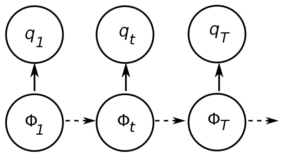
Figure 1Schematic graph of hidden Markov modelling.
The state variable is unobserved and is accordingly referred to as a hidden variable. The hidden state Φt is modelled as a N state Markov chain fully characterized by its transition probability matrix M with elements Mij:
where Mij describes the transition probability to switch from the state i at time t−1 to state j at time t.
The observed variable qt is assumed to have been drawn from a probability distribution whose parameters are conditional upon the distinct state at time t such that, when Φt is known, the distribution of qt depends only on the current state Φt and not on previous states or observations.
A HMM is described by (1) the parameters of Gaussian distributions, i.e. mean and standard deviation associated with N states, (2) the N×N matrix of transition probabilities M, and (3) the initial distribution of the Markov chain δ. Consequently, the set of parameters to be estimated is .
Fitting a HMM to the observed sequence (here the time series of annual flows) requires evaluating the likelihood of observing that sequence, as calculated under an N-state HMM (see Appendix A for more details). In this study, we use the expectation–maximization (EM) algorithm, which is an iterative method for finding the maximum-likelihood estimate of the parameters of an underlying distribution when some of the data are missing. In the context of HMM, the EM algorithm is known as the Baum–Welch algorithm (Welch, 2003), and the hidden climate states are treated as missing data (Bilmes, 1998; Zucchini et al., 2017).
The EM algorithm consists of two main phases: an expectation phase called “E step”, followed by a maximization phase called “M step”. Given the current estimate of the HMM parameters θ, the following steps are repeated until acceptable convergence is achieved: the E step phase of the algorithm computes the expected value of unobserved data (i.e. hidden climate states) using the current estimate of the parameters and the observed data. The M step phase of the algorithm then provides a new estimate of the parameters by using the data from the E step phase as if they were actually measured data. These parameters are then used to calculate the distribution of unobserved data in the next E step phase of the algorithm. The resulting values of θ are then the stationary point of the likelihood of the observed data (please refer to Appendix B for more details).
Given the observation sequence, we want to determine the sequence of hidden climate states that have most likely (under the fitted HMM) given rise to the time series of annual river discharges. In the literature, this is known as the decoding procedure. In this study we use the Viterbi algorithm (Viterbi, 1967) to unfold the sequence of hidden climate states (called the Viterbi path). This, in turn, enables us to divide the whole period into numerous climate subsequences.
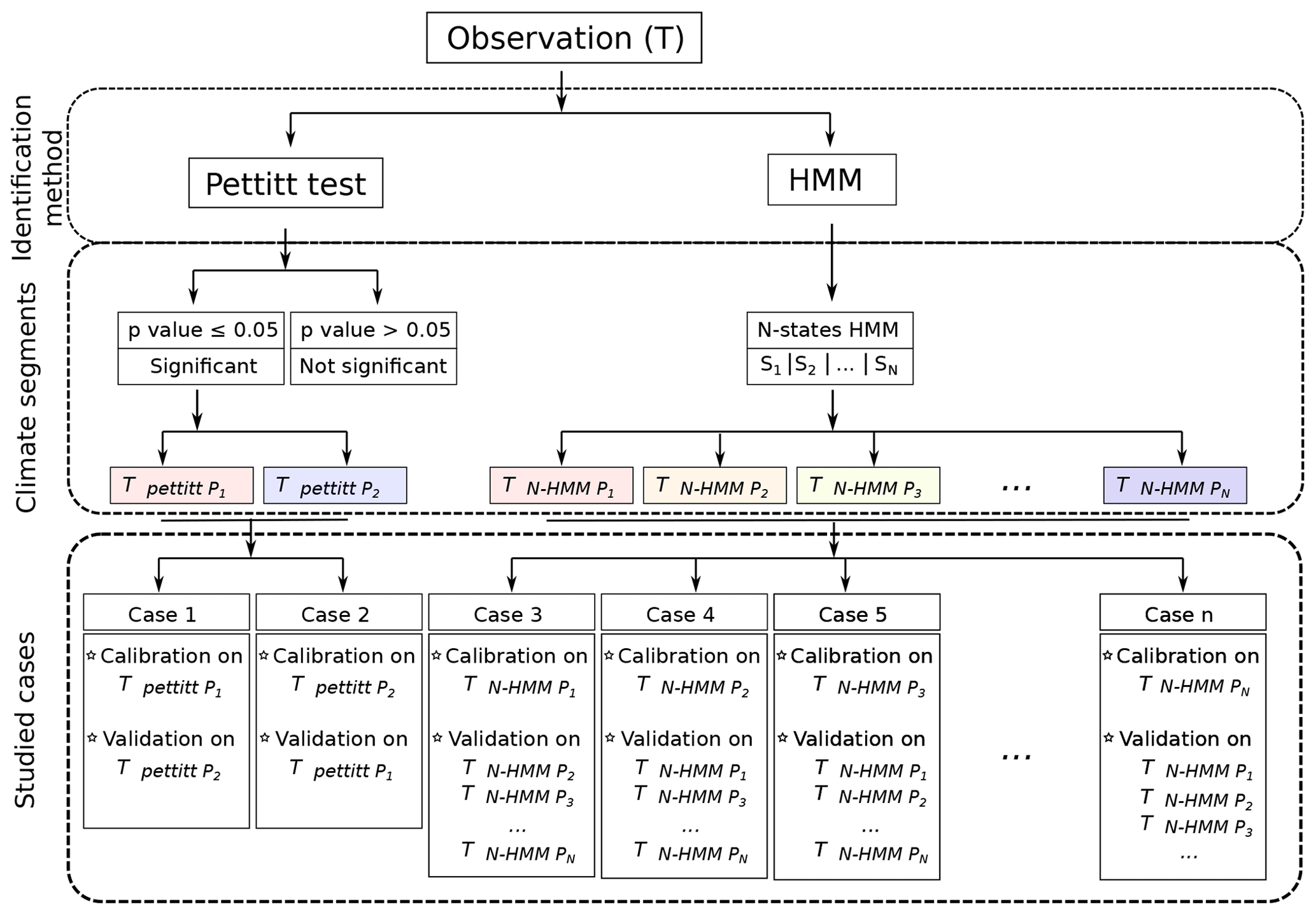
Figure 2Pettitt's test and HMM identifications of flow sequences in a given period T. N refers to the number of states fixed by the modeller and so the number of cases available for the calibration/validation.
Figure 2 depicts the possible combinations offered by Pettitt's test and HMM classifications. The hydrological model is calibrated on a specific subsequence, and the validation is achieved on others. Thus, the model performances (i.e. the robustness) are assessed over a large panel of hydroclimatic conditions. More specifically, the robustness of the hydrological model can be assessed after examining the differences between calibration and validation scores for the different cases (transitions) that can be investigated once the subsequences are identified. If those differences remain stable, then the hydrologic model is robust vis-à-vis contrasted hydroclimatic conditions.
2.3 The study case: Senegal River basin and its sub-basins
The use of HMM-derived subsequences in a differential split-sample testing framework to assess the robustness of a calibrated hydrological model is illustrated with the Senegal River basin.
The Senegal River drains a basin shared by four countries in West Africa : Guinea, Mali, Mauritania, and Senegal. There are three main tributaries: (i) the Bafing River contributing to ∼ 50 % of the Senegal River flows, (ii) the Bakoye River (∼ 15 %), and (iii) the Faleme River (35 %). Flowing northward for 500 km, the Bafing River collects precipitation on the Fouta Djallon, a high plateau considered the water tower of West Africa. After merging with the Bakoye River, the Senegal River runs northwest for 200 km before the confluence with the Faleme River at Bakel, the last major tributary. After Bakel, the river meanders over 800 km through the floodplain and then discharges into the Atlantic Ocean.
The basin is located in the Sudano–Guinean zone, which is yearly influenced by the monsoon, a rainy season from April to October (Lahtela, 2003; Bodian, 2011). A consequence of the monsoon is a strong north–south precipitation gradient, ranging from 1900 mm yr−1 in the south to 100 mm yr−1 in the north (Bader et al., 2014; Bodian et al., 2015). In addition, precipitation present strong annual and inter-annual historical variabilities (Faye et al., 2015), with a wet episode (1950s–1970s) and a dry episode (1970s–1990s). With this historical climatic variability, as well as a strong spatial heterogeneity of its hydroclimatic components, the SRB is an interesting case study to analyze the robustness of hydrological models.
Table 1List of the SRB sub-basins. Superficies have been calculated with the GRASS-3.4 model and 1arc sec SRTM elevation data. Indicative isohyets ranging are extracted from Faye et al. (2015).
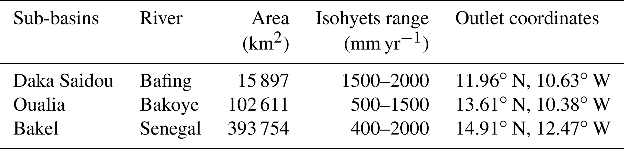
To take advantage of the hydroclimatic specificities of the SRB and its heterogeneity, we have divided the SRB into three sub-basins (Fig. 3b, c, d and Table 1). This allows us to demonstrate the potential of the proposed protocol based on a HMM classification on basins with contrasting hydrologic characteristics. Sub-basins have been delimited using the GRASS-3.4 software and the Shuttle Radar Topography Mission (SRTM) 1 arcsec elevation data set.
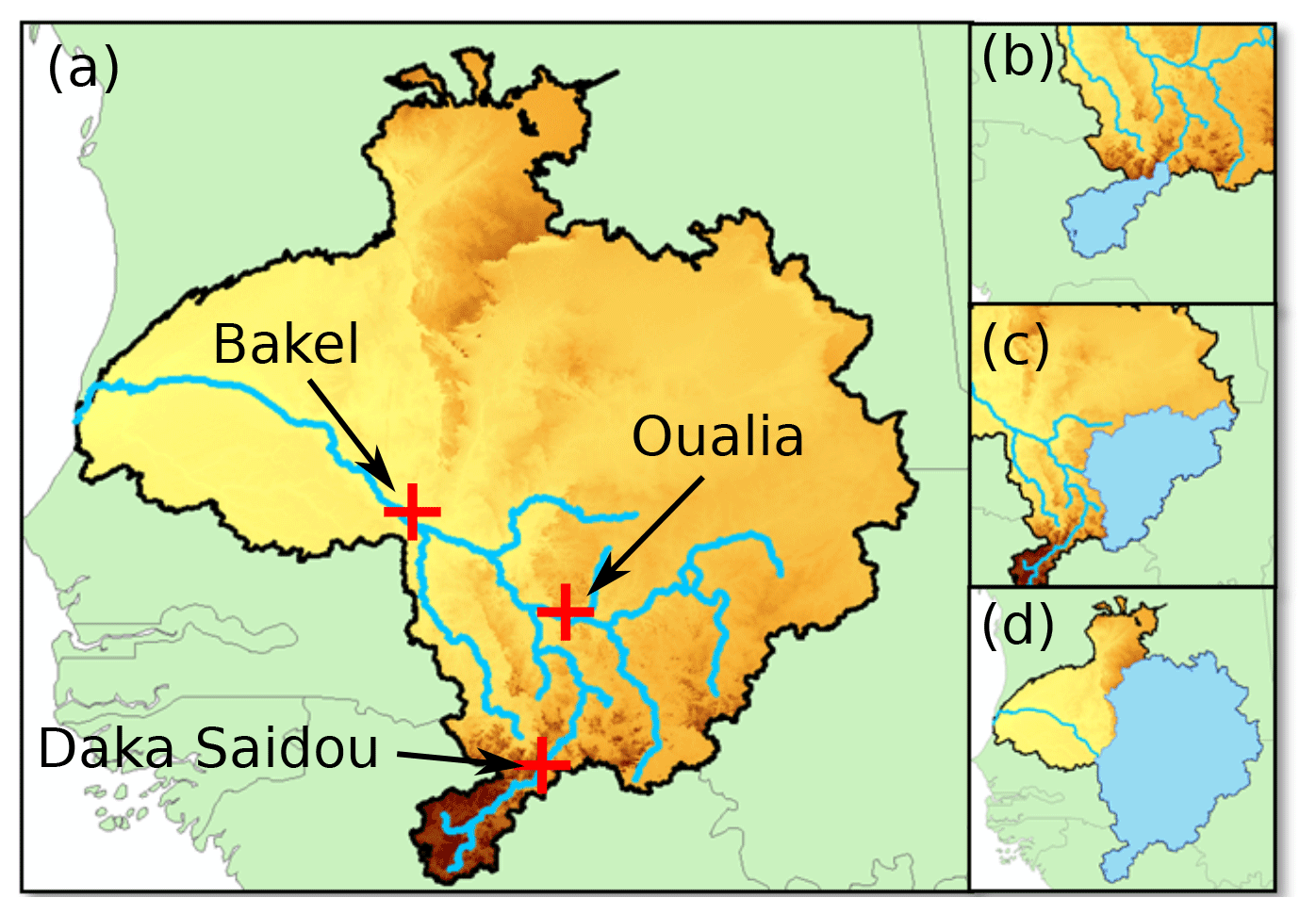
Figure 3The SRB and its sub-basin boundaries. Red crosses represent sub-basin outlets (a), while sub-basin superficies are shaded in blue (b, Daka Saidou; c, Oualia; d, Bakel).
Generally speaking, streamflows are considered an integrative signal of the whole basin hydroclimatic conditions, meaning that river discharges are the result of hydrological processes taking place upstream and are influenced by changes in precipitation, land use, etc. For the Senegal River basin, most of the runoff and headwaters are located in the Fouta Djallon, a sparsely populated plateau where vegetation cover is relatively stable (Descroix et al., 2020) anthropogenic impacts on runoff seem to be negligible (Faty, 2017; Bader et al., 2014; OMVS, 2011). The areas mainly concerned with massive land-use conversions are located downstream of Bakel, a region not considered in our analysis because it marginally contributes to the river discharge. This study relies on a time series of naturalized flows at Bakel produced by Bader et al. (2014) after removing the influence of the Manantali Dam. In Daka Saidou and Oualia sub-basins, however, river discharges are still natural. Consequently, we can assume that changes in the flow regime can only be attributed to shifting climate conditions.
2.4 The selected hydrological model
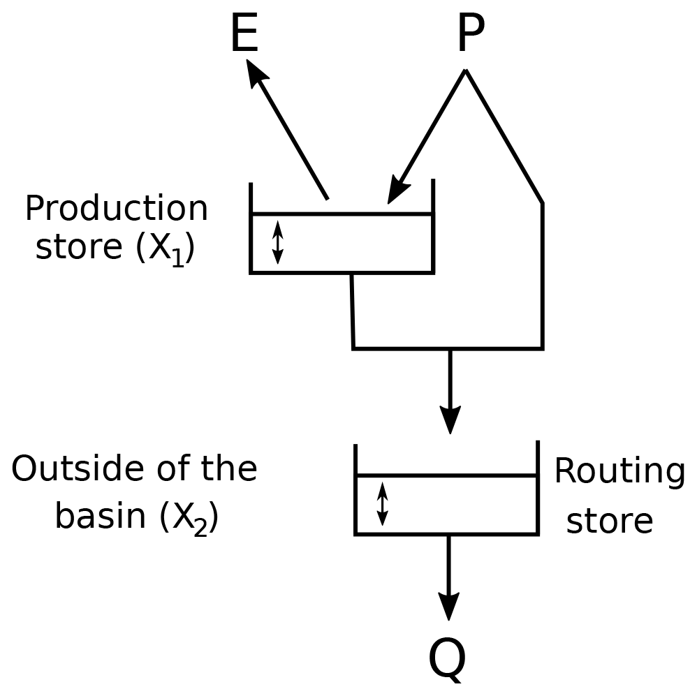
The selected hydrological model is GR2M (Mouelhi, 2003), a monthly time-step conceptual model that has already been used in the SRB with satisfactory results (Ardoin-Bardin, 2004; Ardoin-Bardin et al., 2005; Bodian et al., 2012, 2015, 2016). Moreover, since the simulated flows will be processed by a hydro-economic model of the SRB working on a monthly time step (Tilmant et al., 2020), there was no need for a hydrological model working on a shorter time step.
GR2M has only two parameters: X1 and X2, controlling the production and the transfer functions respectively (Fig. 4). We use the GR2M version included in the environment “airGR”, developed by Coron et al. (2017). The GR2M calibration/validation phase requires three time series: (i) a time series of monthly precipitation (P) in the basin, (ii) a time series of monthly potential evapotranspiration (PET), and (iii) a time series of monthly river discharges (q) at the outlet.
2.5 Implementing the differential split-sample test on HMM-derived subsequences
Many authors have pointed out that selecting the most accurate hydrological and meteorological inputs can significantly reduce the total error during the calibration/validation of a hydrological model (Paturel et al., 1995; Huard and Mailhot, 2006; Kavetski et al., 2006; Huard and Mailhot, 2008; Renard et al., 2010). Based on a comparison with meteorological observations compiled by SIEREM (Système d'Informations Environnementales sur les Ressources en Eau et leur Modélisation) and details given by Bader et al. (2014) about hydrological data, the following dataset is selected: (1) time series of precipitation were extracted from the HSM-SIEREM dataset, stretching from 1940 to 1998 (Boyer et al., 2006); (2) the PET time series comes from the Climate Research Unit (CRU) (Harris et al., 2020) and covers a period from 1901 to 2018; (3) monthly river discharge data at sub-basin outlets are naturalized flows extracted from Bader et al. (2014) for the 1903–2012 period. Based on the above datasets, the analysis is carried out on the period 1940–1998 (59 years), which is denoted by “the full historical record” (T1940–1998) in the remainder of this paper.
Selecting an objective function to calibrate a conceptual hydrological model is one of the main concerns of the hydrological community (Garcia et al., 2017; Krause et al., 2005; Madsen, 2003). Here, two objective functions are selected: (1) the Nash–Sutcliffe efficiency (NSE) (Nash and Sutcliffe, 1970) and the (2) Kling–Gupta efficiency (KGE) (Gupta et al., 2009). The former is a popular criterion, and since it mainly focuses on high flows, it is particularly relevant for rivers where much of the annual discharge is generated during the high-flow season, which is the case in the SRB. The latter allows for a multi-objective calibration that considers more components than just the errors, i.e. correlation, bias, and variability.
Mathematically, the NSE and KGE formulations can be written as
where qobs is the observed flow at time t, qsim is the simulated flow at time t, μobs is the mean of observed flows, β the ratio between the mean simulated flow and the mean observed flow value , α the ratio between the standard deviation of simulated flows and the standard deviation of observed flows , and r is given by

Figure 5Pettitt's test and HMM identifications of flow sequences: seven cases for the calibration/validation phase are obtained (note that “nor” represents normal conditions).
For the identification of the subsequences, we have implemented Pettitt's test, a two-state HMM classification (a dry state and a wet state), and a three-state HMM classification (dry, normal, and wet states). As shown in Fig. 5, seven transitioning cases can be investigated within the differential split-sample testing framework.
-
If relevant, the Pettitt test offers two calibration/validation possibilities: calibration on Tpettitt.dry and validation on Tpettitt.wet (and vice versa).
-
The two-state HMM classification offers two possibilities too: calibration on T2HMM.dry and validation on T2HMM.wet (and vice versa).
-
Similarly, the three-state HMM classification leads to three possibilities: calibration on T3HMM.dry and validation on (and corollaries).
Pettitt test and HMM classifications have been carried out on the time series of annual flows. Tpettitt.wet and Tpettitt.dry are both subsequences made of contiguous years as the original time series is split into two. In that case, the temporal persistence found in the original time series is very much preserved. However, for T2HMM.wet and T2HMM.dry, the situation is different since they are made of numerous, not necessarily contiguous, wet or dry subsequences respectively. This is also true for T3HMM.wet, T3HMM.nor, and T3HMM.dry.
Even though the KGE is based on a decomposition of the NSE, the corresponding scores cannot be directly compared. Therefore, we will discuss the results obtained with NSE and KGE separately. During all calibration phases, the first year is considered warming-up period and not considered. Recall that the identification of change points is done on the time series of annual flows, while the hydrological model simulates monthly river discharges.
First, we applied the calibration/validation protocol on the full historical record (T1940–1998). The results (Sect. 3.1) highlight the relevance of a HMM classification for long time series (59 years) with a historical contrasted climate.
Then, the protocol is implemented, independently, on two shorter periods: 1945–1971 (T1945–1971, 27 years) and 1972–1998 (T1972–1998, 27 years). This second test aims at illustrating the relevance of HMM classifications for shorter time series, which do not display a clear climate trend. Results are respectively given in Sect. 3.2 and 3.3.
3.1 Subsequence identification and calibration/validation results for the full historical record T1940–1998
The results of the division of the full historical record T1940–1998 are displayed in Table 2 and Fig. 6a. Calibration and validation values are given in Fig. 6b and in Table 3.
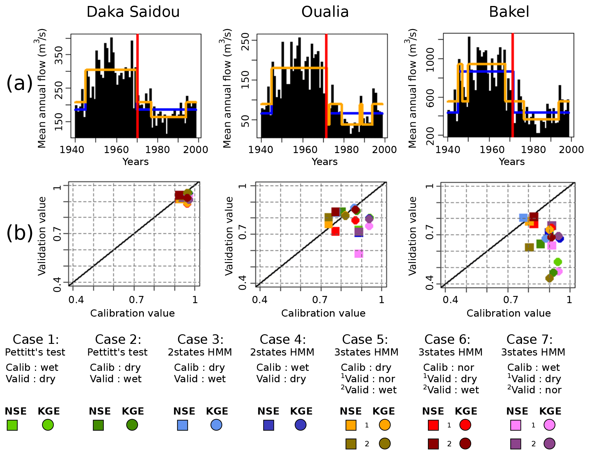
Figure 6The full historical record T1940–1998. (a) Classifications of T1940–1998 according to the Pettitt test (vertical red lines), two-state HMM (in blue), and three-state HMM (in orange); (b) scatterplot of NSE (squares) and KGE (dots) calibration/validation values. The continuous black line refers to the CalibrationValue=ValidationValue line.
Table 2Pettitt test results and hidden Markov model parameters (N=2 and N=3) for Daka Saidou, Oualia, and Bakel sub-basins, on the full historical record T1940–1998.
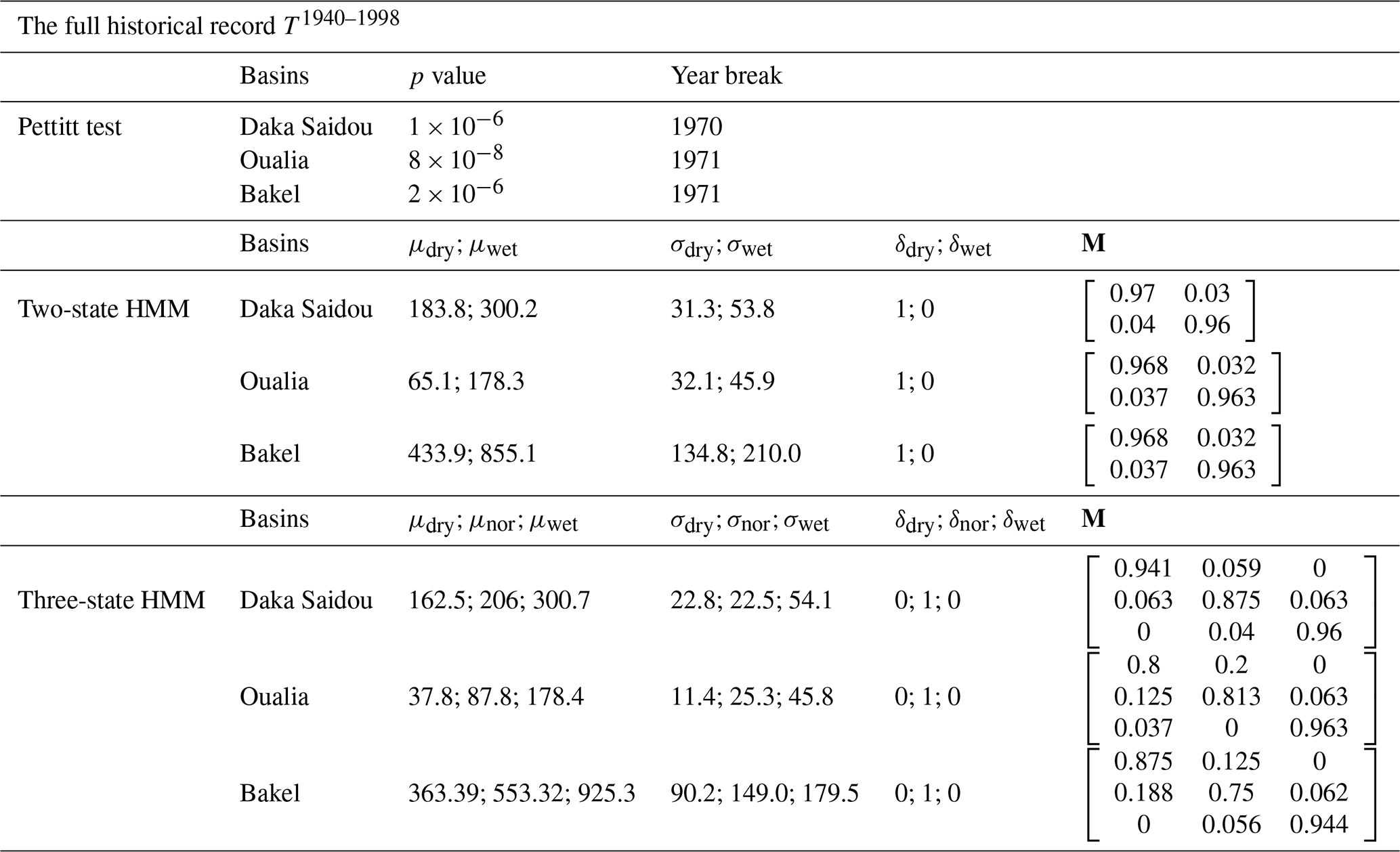
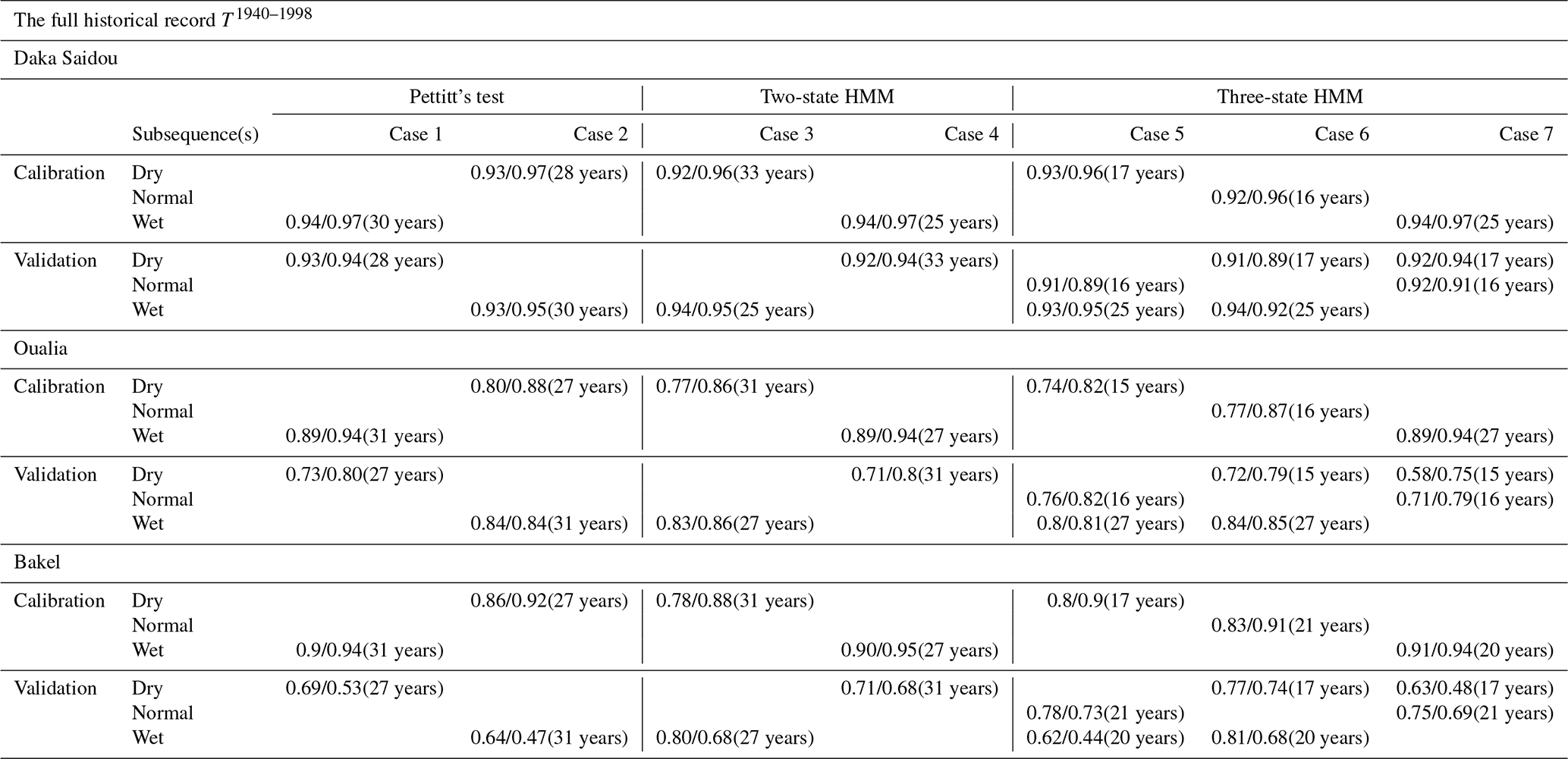
Table 3Table of NSE/KGE calibration and validation scores according to the seven cases for the full historical record T1940–1998. The numbers of years used for the calibration or validation are given in parenthesis.
For the three sub-basins, Pettitt's test is significant and shows a rupture in 1970 or 1971 (Table 2, Fig. 6a vertical red line). The two-state HMM classification provides similar results with nearly aligned climate subsequences for all sub-basins. This is also true for the three-state HMM classification. It must also be noted that Pettitt's test-derived and HMM-derived subsequences are quite long, ranging from 15 to 33 years.
From the examination of the transition probability matrices M in Table 2, we can see that the states are clearly distinct both with the two-state and the three-state HMM classification. As a matter of fact, the values close to one on the diagonal indicate that when the climate is in a particular state, it will likely remain in that state in the next time period (year).
The examination of Fig. 6b reveals that, for Daka Saidou (upstream), the model's scores (NSE or KGE) in calibration and validation are gathered in the top right corner, indicating that the model is able to reproduce well the subsequences of the historical record that have been used in calibration and then in validation. A statistical analysis of the subsequences shows that those sharing the same (hidden) climate state have similar statistics, but the differences across climate states are relatively small at Daka Saidou compared to the other two sub-basins located downstream (Bakel and Oualia). For example, the mean monthly streamflows of dry subsequences represent 64 %, 61 %, and 54 % of wet subsequences for the Pettitt test two-state-HMM and three-state-HMM classification respectively, which, as we will see later, are much higher ratios than those found at Bakel or Oualia. In other words, although the climate subsequences are indeed statistically distinct, they are nevertheless not that far apart, meaning that, regardless of the transitions, the conditions for calibration and validation are not significantly different.
For Oualia and Bakel sub-basins, however, calibration/validation scores are more scattered; only some model versions are able to perform consistently over contrasted climates. For Oualia, calibrations on dry and normal subsequences (cases 2, 3, 5, and 6) provide relatively good values and similar validation scores (difference between calibration and validation scores lower than 0.1), meaning that the associated model versions could be considered robust. Those results suggest that the “wet version” of the model struggles to simulate very dry months (especially during the dry subsequences). It seems that the wet version of the model does not handle well the intermittent streams which can be observed in the northern (driest) part of Oualia sub-basin during dry years. For Bakel, we can see that the calibration/validation scores obtained from the HMM-derived wet and dry subsequences (cases 3 and 4) are systematically better than those calculated for the subsequences identified by the Pettitt test (cases 1 and 2). Here, calibrating on dry conditions and validating on wet conditions do not systematically perform better than the other way around. In contrast to Oualia, Bakel sub-basin drains a portion of the Fouta Djallon with the Faleme and Bafing rivers and is therefore less sensitive to those intermittent streams found in the north. Finally, as we move downstream, we can see that the difference between the NSE and KGE scores tends to increase. As pointed out by Gupta et al. (2009), since the NSE uses the observed mean as baseline, it can lead to overestimation of model skill for highly seasonal time series. Here, due to the north–south precipitation gradient, the seasonality of the flow regime increases once the river leaves the Fouta Djallon since it receives the contribution of more and more intermittent tributaries.
3.2 Subsequence identification and calibration/validation results for T1945–1971
This section examines the period 1945–1971 (T1945–1971), which can be considered a wet historical episode in the SRB. The results of the division are displayed in Table 4 and Fig. 7a. Calibration and validation values are given in Fig. 7b and in Table 5.
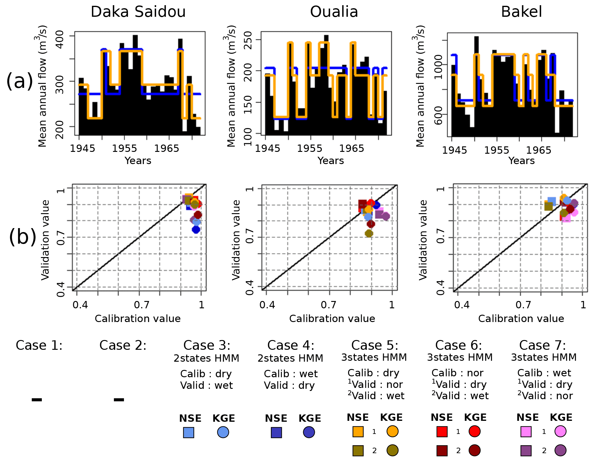
Figure 7The wet subsequence T1945–1971. The caption is identical to the caption of Fig. 6 but for the T1945–1971 period.
Table 4Pettitt test results and hidden Markov model parameters (N=2 and N=3) for Daka Saidou, Oualia, and Bakel sub-basins, on the wet subsequence T1945–1971.
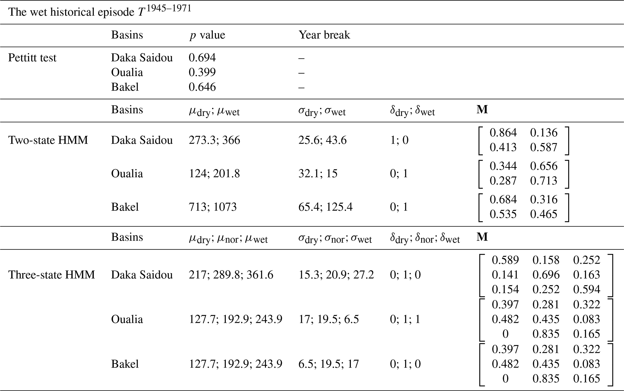
Table 5Table of NSE/KGE calibration and validation scores according to the seven cases for the wet subsequence T1945–1971. As Pettitt's test is not conclusive here, no calibration/validation scores are given (symbols ).

For the three sub-basins, Pettitt's tests are inconclusive, indicating that there is no clear climatic trend in the T1945–1971 period. However, the HMM is still able to make the distinction between climate states and thus identify corresponding subsequences, which can then be exploited in a differential split-sample test. The subsequences provided by two-state-HMM and the three-state-HMM classifications are not necessary aligned for all sub-basins. As T1945–1971 is a 26-year period, the two-state-HMM-derived and the three-state-HMM-derived subsequences have lengths ranging from 5 to 19 years. Various authors have discussed the minimum length required to achieve a calibration or a validation without reaching a consensus, even though a number from 2 to 8 years could be enough depending on the “hydrological events” included in the subsequences (Razavi and Coulibaly, 2013; Juston et al., 2009; Singh and Bárdossy, 2012). In our case, the technique used to identify the subsequences (HMM classifications) seeks to provide relatively homogeneous ones. Here, we assume that 5 years is acceptable, but we do not investigate this issue further since it is beyond the scope of our paper.
The transition probability matrices for the two-state HMM and three-state HMM are now diverging from an identity matrix, indicating that the temporal persistence is less pronounced than that found in the full historical records. In addition, we note that the mean annual flow of dry subsequences ( and ) are relatively high (in comparison with and ).
Compared to the results associated with the full historical records and discussed in the previous section, we can see that the calibration/validation scores for the five remaining cases are more concentrated, especially for the two downstream sub-basins (Oualia and Bakel). During this wet episode, the hydrological models seem to be more robust, which is consistent with the fact that the intrinsic variability of the hydrologic conditions within that episode is smaller than the variability that characterizes the full historical records. With the north–south gradient that characterizes precipitation in the SRB, intermittent tributaries in the north under dry or normal conditions are turned into permanent rivers which are better handled by conceptual models like GR2M.
3.3 Subsequence identification and calibration/validation results for T1972–1998
Here, we focus on the period 1972–1998 (T1972–1998), which can be considered a dry historical episode in the SRB. The results of the division and the corresponding parameters are displayed in Table 6 and Fig. 8a. Calibration and validation values are given in Fig. 8b and in Table 7.
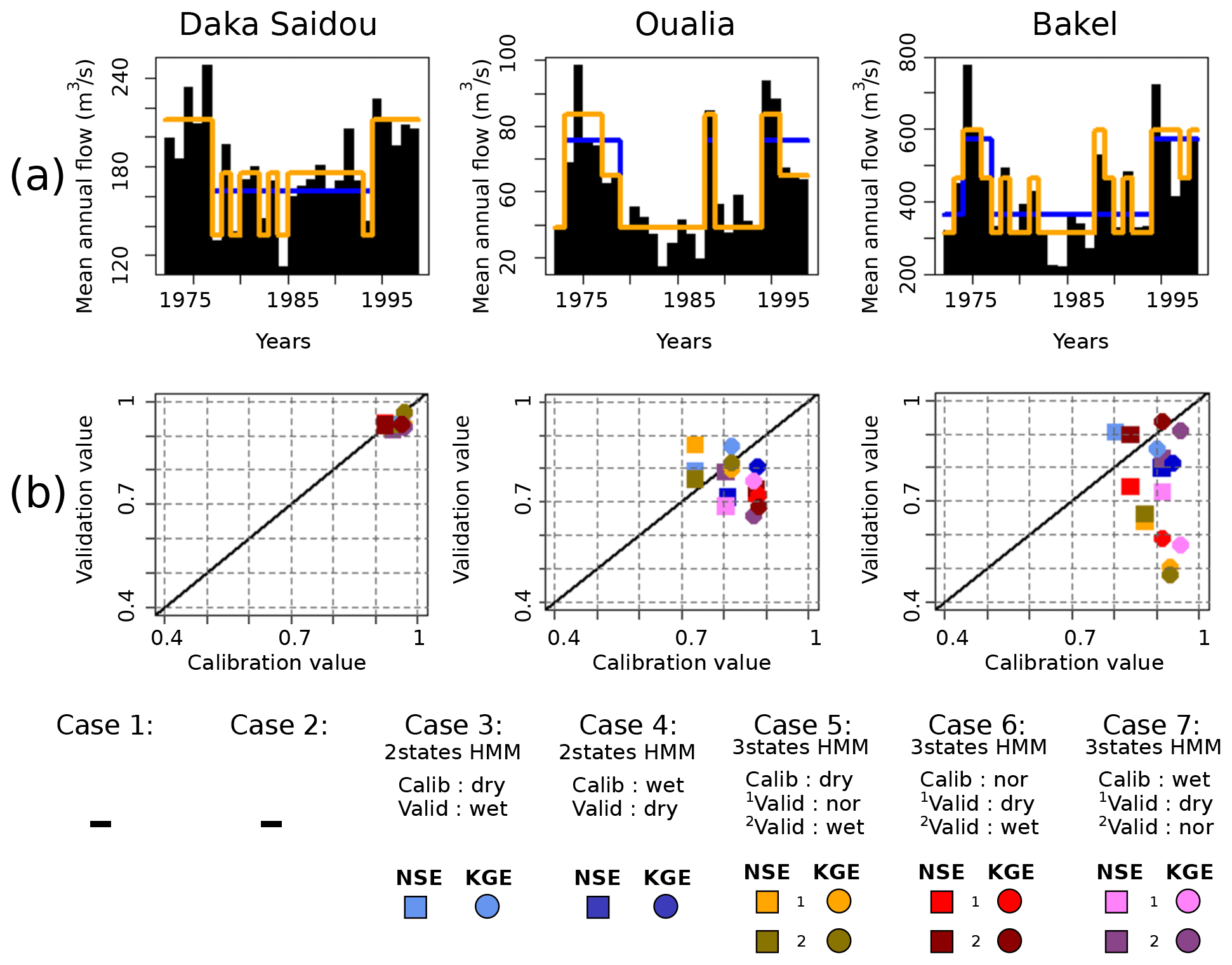
Figure 8The dry subsequence T1972–1998. The caption is identical to the caption of Fig. 6 but for the T1972–1998 period.
Table 6Pettitt test results and hidden Markov model parameters (N=2 and N=3) for Daka Saidou, Oualia, and Bakel sub-basins, on the dry subsequence T1972–1998.
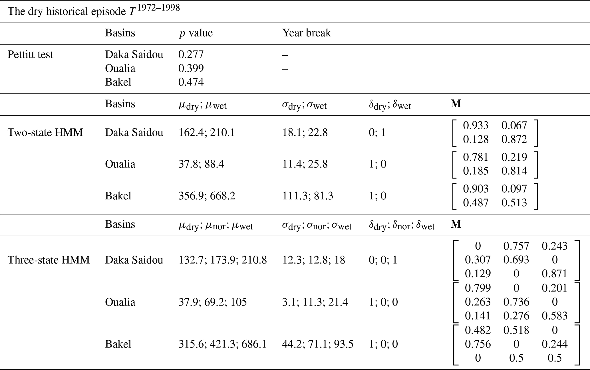
Table 7Table of NSE/KGE calibration and validation scores according to the seven cases for the dry subsequence T1972–1998. As Pettitt's test is not conclusive here, no calibration/validation scores are given (symbols ).

Likewise in Sect. 3.2, there is no clear monotonic climatic trend such as Pettitt's test is inconclusive (p values bigger than 0.05). Again, the HMM remains here a useful tool to identify subsequences, which are not necessary aligned for all sub-basins.
For Daka Saidou, all calibration and validation scores are higher than 0.9, and the differences are small (below 0.1). For Oualia sub-basin, the calibration and validation of the hydrological model face the typical challenges associated with the high spatial and temporal variability that characterizes the formation and propagation of river flows in dryland regions. The dry episode, centered around the 1980s, was triggered by a sustained reduction in precipitation (Faye et al., 2015), which was even more pronounced in the north where some tributaries became intermittent rivers (Bader et al., 2014). Conceptual hydrological models like GR2M are indeed not well equipped to deal with sudden and widespread transitions from wet to dry conditions (Gutierrez-Jurado et al., 2021). For Bakel, no clear pattern emerges: some “dry versions” have as bad (or good) performances as some “wet versions”. The poorest scores are nevertheless obtained when the calibration and validation are carried out on homogeneous subsequences associated with extreme climate states (dry–wet, wet–dry), e.g. cases 5–2 and 7–1.
This article proposes a HMM-based classification to deal with complex climate sequences and shows how the resulting classification can be used in a differential split-sample test to assess the robustness of a hydrological model. A modelling experiment is carried out in the Senegal River basin using the GR2M model and historical flows from 1940–1998. Then, two other periods have been investigated: a wet episode (1945–1971) and a dry one (1972–1998).
The main concluding remarks are the following:
-
When records display a single point change, a classical rupture trend (as Pettitt test) remains an adequate tool to divide the records into two climate subsequences.
-
If the records contain multiple change points, a HMM classification can divide the series into several climate subsequences without the need for additional data.
-
Regardless of the division method used, the range of climate conditions over which the hydrological model can perform depends on the intrinsic variability of the series. Compared to the Pettitt test, however, the HMM classification allows for a finer labelling of the years and therefore better exploiting the intrinsic variability in the series to enrich a differential split-sample test.
-
We encourage modellers to explore as many cases as possible to calibrate/validate a hydrological model according to the differential split-sample test. The parameter's stability over contrasted hydroclimatic conditions seems to depend on the studied period, on the objective functions, on the subsequence identification techniques, and on the basin.
We suppose there is an observation sequence and the associated (unobserved) state variables generated by such a model. Given the set of HMM parameters , the joint density of complete data set can be expressed as
Assuming the data belonging to each hidden state are characterized by a specific Gaussian probability distribution, the two terms on the right-hand side are
The complete data likelihood function ζ(θ|Z) can be calculated as
For a HMM which has the initial distribution δ and transition probability matrix M for the Markov chain, let us define the probability mass function of Q if the Markov chain is in state i at time t as
with .
The general form of likelihood function is then given by the following (Zucchini et al., 2017):
where Γ(q) is defined as the diagonal matrix with i being the diagonal element pi(q) and 1′ being an N dimensional vector of 1.
In order to set out the likelihood computation in the form of the Baum–Welch algorithm (Welch, 2003), which involves the forward α(t) and backward β(t) probabilities, we define α(t) and β(t) as
and
respectively. More specifically, αi(t) is the probability of observing the partial sequence and ending up in state i at time t, and βi(t) is the probability of observing the remaining sequence. Numerical calculation of αi(t) and βi(t) is not trivial (Akintug and Rasmussen, 2005). Here we use the method suggested by Durbin et al. (1998) for scaling forward and backward probabilities to overcome this problem. Now let us define uj(t) and vjk(t) as the following (Zucchini et al., 2017):
where Mjk is the probability of transition from hidden climate state j to climate state k, and ζ is the likelihood function. With EM algorithm, we aim to maximize the log-likelihood of the parameters of interest θ, based on complete data (i.e. both the observed data and the hidden climate states). Now let us represent the sequence of climate states (missing data) by the Markov chain by the zero–one random variables. The complete data log-likelihood can be formulated as
where uj(t)=1 if and only if , and transition probability vjk(t)=1 if and only if and ; N is the number of hidden climate states, δj is the initial transition of Markov chain, and pj(.) is the probability mass function if the Markov chain is in state j at time t. Maximization of the complete data log-likelihood function is performed with the EM algorithm through an iterative process presented in Fig. B1.

Precipitation and potential evapotranspiration data can be retrieved respectively from SIEREM (Système d'Informations Environnementales sur les Ressources en Eau et leur Modélisation: http://www.hydrosciences.fr/sierem/produits/Grilles/GrillesIRD.asp, IRD – HSM, 2021) and from CRU (Climate Research Unit: https://crudata.uea.ac.uk/cru/data/hrg/; Harris et al., 2020). Streamflow data are available at https://www.documentation.ird.fr/hor/fdi:010065190 (Bader et al., 2014). The code for HMM classification is available on GitHub (https://github.com/Vahidesp/HMM_Classification.git, last access: 15 August 2021; https://doi.org/10.5281/zenodo.5172027, Espanmanesh, 2021). The GR2M code is embedded into the “airGR” R package (https://cran.r-project.org/web/packages/airGR/index.html, Coron et al., 2021).
EG was in charge of the data curation, the formal analysis, the investigation, the methodology develpoment, the software coding, the validation, the original draft writing, as well as the reviewing and editing steps. VE contributed to the data curation, the methodology, the software coding, the validation and the writing. AT contributed to the conceptualization, the funding acquisition, the methodology, the project administration, the supervision, the validation, and the writing. FA contributed to conceptualization and the writing.
The authors declare that they have no conflict of interest.
Publisher’s note: Copernicus Publications remains neutral with regard to jurisdictional claims in published maps and institutional affiliations.
The authors thank the reviewers, the associate editor and editor for their constructive comments.
This research has been supported by the Food and Agriculture Organization of the United Nations (FAO, project SAGA “Sécurité Alimentaire: une Agriculture adaptée”) and the Natural Sciences and Engineering Research Council of Canada (NSERC).
This paper was edited by Fabrizio Fenicia and reviewed by two anonymous referees.
Akintug, B. and Rasmussen, P. F.: A Markov switching model for annual hydrologic time series, Water Resour. Res., 41, 1–10, https://doi.org/10.1029/2004WR003605, 2005. a, b
Ardoin-Bardin, S.: Variabilité hydroclimatique et impacts sur les ressources en eau de grands bassins hydrographiques en zone soudano-sahélienne, PhD thesis, Université Montpellier II, https://doi.org/10.1038/ni.2208, 2004 (in French). a
Ardoin-Bardin, S., Dezetter, A., Servat, E., and Mahe, G.: Évaluation des impacts du changement climatique sur les ressources en eau d'Afrique de l'Ouest et Centrale, in: Regional Hydrological Impacts of Climatic Change – Hydroclimatic Variability, IAHS, Foz de Iguaçu, Brazil, 194–202, 2005 (in French). a
Bader, J.-C., Cauchy, S., Duffar, L., and Saura, P.: Monographie hydrologique du fleuve Sénégal. De l'origine des mesures jusqu'en 2011, IRD, Marseille (France), IRD edition, available at: https://www.documentation.ird.fr/hor/fdi:010065190 (last access: 1 July 2021), 2014 (in French). a, b, c, d, e, f, g
Bernier, J.: Etude de la stationnarité des séries hydroméléorologiques, La houille blanche, 4, 313–219, 1977 (in French). a
Bilmes, J. A.: A gentle tutorial of the EM algorithm and its application to parameter estimation for Gaussian mixture and hidden Markov models, Tech. Rep. 510, International Computer Science Institute, Berkeley, https://doi.org/10.1080/0042098032000136147, 1998. a
Bodian, A.: Approche par modélisation pluie – débit de la connaissance régionale de la ressource en eau : Application au haut bassin du fleuve Sénégal, PhD thesis, Université Cheikh Anta Diop de Dakar, available at: http://hydrologie.org/THE/BODIAN.pdf (last access: 1 July 2021), 2011 (in French). a
Bodian, A., Dezetter, A., and Dacosta, H.: Apport De La Modélisation Pluie-Débit Pour La Connaissance De La Ressource En Eau: Application Au, Climatologie, 9, 109–125, https://doi.org/10.4267/climatologie.223, 2012 (in French). a
Bodian, A., Dezetter, A., and Dacosta, H.: Rainfall-runoff modelling of water resources in the upper Senegal River basin, Int. J. Water Resour. D., 32, 89–101, https://doi.org/10.1080/07900627.2015.1026435, 2015. a, b
Bodian, A., Dezetter, A., Deme, A., and Diop, L.: Hydrological evaluation of TRMM Rainfall over the Upper Senegal River basin, Hydrology, 3, 1–18, https://doi.org/10.3390/hydrology3020015, 2016. a
Borgomeo, E., Hall, J. W., Fung, F., Watts, G., Colquhoun, K., and Lambert, C.: Risk-based water resources planning: Incorporating probabilistic nonstationary climate uncertainties, Water Resour. Res., 50, 6850–6873, https://doi.org/10.1002/2014WR015558, 2014. a
Boyer, J. F., Dieulin, C., Rouche, N., Cres, A., Servat, E., Paturel, J. E., and Mahé, G.: SIEREM: An environmental information system for water resources, in: FRIEND World Conference, November 2006, Havana, Cuba, IAHS, 308, 19–25, 2006. a
Bracken, C., Rajagopalan, B., and Zagona, E.: A hidden Markov model combined with climate indices for multidecadal streamflow simulation, Water Resour. Res., 50, 7836–7846, https://doi.org/10.1002/2014WR015567, 2014. a
Brigode, P., Oudin, L., and Perrin, C.: Hydrological model parameter instability: A source of additional uncertainty in estimating the hydrological impacts of climate change?, J. Hydrol., 476, 410–425, https://doi.org/10.1016/j.jhydrol.2012.11.012, 2013. a, b
Brown, C. and Wilby, R. L.: An alternate approach to assessing climate risks, Eos, 93, 401–402, https://doi.org/10.1029/2012EO410001, 2012. a
Coron, L., Thirel, G., Delaigue, O., Perrin, C., and Andréassian, V.: The suite of lumped GR hydrological models in an R package, Environ. Model. Softw., 94, 166–171, https://doi.org/10.1016/j.envsoft.2017.05.002, 2017. a
Coron, L., Delaigue, O., Thirel, G., Dorchies, D., Perrin, C., Michel, C., Andréassian, V., Bourgin, F., Brigode, P., Le Moine, N., Mathevet, T., Mouelhi, S., Oudin, L., Pushpalatha, R., and Valéry, A.: airGR: Suite of GR Hydrological Models for Precipitation-Runoff Modelling, available at: https://cran.r-project.org/web/packages/airGR/index.html, last access: 1 July 2021. a
Dacosta, H., Kandia, K. Y., and Malou, R.: La variabilité spatio-temporelle des précipitations au Sénégal depuis un siècle, Regional Hydrology: Bridging Ihe Gap between Research and Practice (Proceedings), 274, 499–506, 2002 (in French). a
Dakhlaoui, H., Ruelland, D., and Tramblay, Y.: A bootstrap-based differential split-sample test to assess the transferability of conceptual rainfall-runoff models under past and future climate variability, J. Hydrol., 575, 470–486, https://doi.org/10.1016/j.jhydrol.2019.05.056, 2019. a
Descroix, L., Faty, B., Manga, S. P., Diedhiou, A. B., Lambert, L. A., Soumaré, S., Andrieu, J., Ogilvie, A., Fall, A., Mahé, G., Diallo, F. B. S., Diallo, A., Diallo, K., Albergel, J., Tanimoun, B. A., Amadou, I., Bader, J. C., Barry, A., Bodian, A., Boulvert, Y., Braquet, N., Couture, J. L., Dacosta, H., Dejacquelot, G., Diakité, M., Diallo, K., Gallese, E., Ferry, L., Konaté, L., Nnomo, B. N., Olivry, J. C., Orange, D., Sakho, Y., Sambou, S., and Vandervaere, J. P.: Are the fouta djallon highlands still the water tower of west africa?, Water, 12, 2968, https://doi.org/10.3390/w12112968, 2020. a, b
Durbin, R., Eddy, S. R., Krogh, A., and Mitchison, G.: Biological Sequence Analysis, Biological Sequence Analysis, Cambridge University press, Cambridge, UK, 1–366, https://doi.org/10.1017/cbo9780511790492, 1998. a
Espanmanesh, V.: Vahidesp/HMM_Classification: HMM Classifications (Version_Final), Zenodo [code], https://doi.org/10.5281/zenodo.5172027, 2021. a
Falkenmark, M., Wang-Erlandsson, L., and Rockström, J.: Understanding of water resilience in the Anthropocene, J. Hydrol., 2, 100009, https://doi.org/10.1016/j.hydroa.2018.100009, 2019. a
Faty, A.: Modélisation hydrologique du haut bassin versant du fleuve Sénégal dans un contexte de variabilité hydro-climatique: Apport de la télédétection et du modèle Mike SHE, PhD thesis, Université de Cheikh Anta Diop de Dakar, Dakar, Senegal, 2017 (in French). a, b
Faye, C., Diop, E. H. S., and Mbaye, I.: Impacts des changements de climat et des aménagements sur les ressources en eau du fleuve sénégal: Caractérisation et évolution des régimes hydrologiques de sous-bassins versants naturels et aménagés, Belgeo – Revue belge de géographie, 4, 1–25, https://doi.org/10.4000/belgeo.17626, 2015 (in French). a, b, c, d
Fortin, L. G., Turcotte, R., Pugin, S., Cyr, J. F., and Picard, F.: Impact des changements climatiques sur les plans de gestion des lacs Saint-François et Aylmer au sud du Québec, Can. J. Civil Eng., 34, 934–945, https://doi.org/10.1139/L07-030, 2007 (in French). a
Garcia, F., Folton, N., and Oudin, L.: Which objective function to calibrate rainfall–runoff models for low-flow index simulations?, Hydrolog. Sci. J., 62, 1149–1166, https://doi.org/10.1080/02626667.2017.1308511, 2017. a
Gleeson, T., Wang‐Erlandsson, L., Porkka, M., Zipper, S. C., Jaramillo, F., Gerten, D., Fetzer, I., Cornell, S. E., Piemontese, L., Gordon, L. J., Rockström, J., Oki, T., Sivapalan, M., Wada, Y., Brauman, K. A., Flörke, M., Bierkens, M. F. P., Lehner, B., Keys, P., Kummu, M., Wagener, T., Dadson, S., Troy, T. J., Steffen, W., Falkenmark, M., and Famiglietti, J. S.: Illuminating water cycle modifications and Earth system resilience in the Anthropocene, Water Resour. Res., 56, 1–24, https://doi.org/10.1029/2019WR024957, 2020. a
Gupta, H. V., Kling', H., Yilmaz, K. K., and Martinez-Baquero, G. F.: Decomposition of the Mean Squared Error & NSE Performance Criteria: Implications for Improving Hydrological Modelling, J. Hydrol., 377, 80–91, https://doi.org/10.1016/j.jhydrol.2009.08.003, 2009. a, b
Gutierrez-Jurado, K. Y., Partington, D., and Shanafield, M.: Taking theory to the field: streamflow generation mechanisms in an intermittent, Mediterranean catchment, Hydrol. Earth Syst. Sci. Discuss. [preprint], https://doi.org/10.5194/hess-2020-659, in review, 2021. a
Harris, I., Osborn, T. J., Jones, P., and Lister, D.: Version 4 of the CRU TS monthly high-resolution gridded multivariate climate dataset, Sci. Data, 7, 109, https://doi.org/10.1038/s41597-020-0453-3, 2020 (data available at: https://crudata.uea.ac.uk/cru/data/hrg/, last access: 1 July 2021). a, b
Huang, S., Shah, H., Naz, B. S., Shrestha, N., Mishra, V., Daggupati, P., Ghimire, U., and Vetter, T.: Impacts of hydrological model calibration on projected hydrological changes under climate change – a multi-model assessment in three large river basins, Climatic Change, 163, 1143–1164, https://doi.org/10.1007/s10584-020-02872-6, 2020. a
Huard, D. and Mailhot, A.: A Bayesian perspective on input uncertainly in model calibration: Application to hydrological model “abc”, Water Resour. Res., 42, 1–14, https://doi.org/10.1029/2005WR004661, 2006. a
Huard, D. and Mailhot, A.: Calibration of hydrological model GR2M using Bayesian uncertainty analysis, Water Resour. Res., 44, 1–19, https://doi.org/10.1029/2007WR005949, 2008. a
IRD (Institut pour la Recherche et le Développement) – HSM (Hydroscience Montpellier): Grilles de pluies mensuelles IRD-HSM, available at: http://www.hydrosciences.fr/sierem/produits/Grilles/GrillesIRD.asp, last access: 1 July 2021. a
Juston, J., Seibert, J., and Johansson, P.: Temporal sampling strategies and uncertainty in calibrating a conceptual hydrological model for a small boreal catchment, Hydrol. Process., 23, 3093–3109, https://doi.org/10.1002/hyp.7421, 2009. a
Kavetski, D., Kuczera, G., and Franks, S. W.: Bayesian analysis of input uncertainty in hydrological modeling: 2. Application, Water Resour. Res., 42, 1–10, https://doi.org/10.1029/2005WR004376, 2006. a
Kendall, M.: Rank correlation methods, Charles Griffin & Co. Ltd., London, UK, 1948. a
Klemes, V.: Operational testing of hydrological simulation models, Hydrolog. Sci. J., 31, 13–24, https://doi.org/10.1080/02626668609491024, 1986. a, b, c
Krause, P., Boyle, D. P., and Bäse, F.: Comparison of different efficiency criteria for hydrological model assessment, Adv. Geosci., 5, 89–97, https://doi.org/10.5194/adgeo-5-89-2005, 2005. a
Lahtela, V.: Managing the Senegal River: National and local development dilemma, Int. J. Water Resour. D., 19, 279–293, https://doi.org/10.1080/0790062032000089365, 2003. a
Lempert, R. J., Groves, D. G., Popper, S. W., and Bankes, S. C.: A general, analytic method for generating robust strategies and narrative scenarios, Manage. Sci., 52, 514–528, https://doi.org/10.1287/mnsc.1050.0472, 2006. a, b
Liu, Q., Wan, S., and Gu, B.: A Review of the Detection Methods for Climate Regime Shifts, Discrete Dyn. Nat. Soc., 2016, 1–10, https://doi.org/10.1155/2016/3536183, 2016. a
Ludwig, R., May, I., Turcotte, R., Vescovi, L., Braun, M., Cyr, J.-F., Fortin, L.-G., Chaumont, D., Biner, S., Chartier, I., Caya, D., and Mauser, W.: The role of hydrological model complexity and uncertainty in climate change impact assessment, Adv. Geosci., 21, 63–71, https://doi.org/10.5194/adgeo-21-63-2009, 2009. a
Madsen, H.: Parameter estimation in distributed hydrological catchment modelling using automatic calibration with multiple objectives, Adv. Water Resour., 26, 205–216, https://doi.org/10.1016/S0309-1708(02)00092-1, 2003. a
Mann, H.: Non parametric tests against trend, Econometrica, 13, 245–259, https://doi.org/10.2307/1907187, 1945. a
Milly, P. C. D., Betancourt, J., Falkenmark, M., Hirsch, R. M., Kundzewicz, Z. W., Lettenmaier, D. P., and Stouffer, R. J.: Stationarity Is Dead: Whither Water Management?, Science, 319, 573–574, https://doi.org/10.1126/science.1151915, 2008. a
Motavita, D. F., Chow, R., Guthke, A., and Nowak, W.: The comprehensive differential split-sample test: A stress-test for hydrological model robustness under climate variability, J. Hydrol., 573, 501–515, https://doi.org/10.1016/j.jhydrol.2019.03.054, 2019. a
Mouelhi, S.: Vers une chaîne cohérente de modèles pluie-débit conceptuels globaux aux pas de temps pluriannuel, annuel, mensuel et journalier, PhD thesis, Université Paris VI, Ecole des Mines de Paris, available at: https://pastel.archives-ouvertes.fr/tel-00005696/document (last access: 30 July 2021), 2003 (in French). a
Naghettini, M.: Fundamentals of Statistical Hydrology, Springer, Cham, Switzerland, https://doi.org/10.1007/978-3-319-43561-9, 2017. a
Nalley, D., Adamowski, J., Biswas, A., Gharabaghi, B., and Hu, W.: A multiscale and multivariate analysis of precipitation and streamflow variability in relation to ENSO, NAO and PDO, J. Hydrol., 574, 288–307, https://doi.org/10.1016/j.jhydrol.2019.04.024, 2019. a
Nash, J. and Sutcliffe, J.: Nash and Sutcliffe – 1970 – River flow forecasting though conceptual models Part 1 – A discussion of principles, J. Hydrology, 10, 282–290, 1970. a
OMVS: SDAGE – Schéma directeur, Tech. rep., OMVS, Organisme de Mise en Valeur du fleuve Sénégal, Dakar, Senegal, 2011. a
Paturel, J. E., Servat, E., and Vassiliadis, A.: Sensitivity of conceptual rainfall-runoff algorithms to errors in input data – case of the GR2M model, J. Hydrol., 168, 111–125, https://doi.org/10.1016/0022-1694(94)02654-T, 1995. a
Paturel, J.-E., Ibrehim, B., and L'Aour, A.: Evolution de la pluviométrie annuelle en Afrique de l'Ouest et centrale au XXeme siècle, Sud Sciences et technologies, 13, 40–46, 2004 (in French). a
Payrastre, O.: Utilité de l'information historique pour l'étude du risque de crues, in: 14èmes Journées Scientifiques de l'Environnement: l'Eau, la Ville, la Vie, edited by: Thévenot, D. R., Créteil, France, available at: https://hal.archives-ouvertes.fr/hal-00203088 (last access: 1 July 2021), 2003 (in French). a
Peel, M. C. and Blöschl, G.: Hydrological modelling in a changing world, Prog. Phys. Geogr., 35, 249–261, https://doi.org/10.1177/0309133311402550, 2011. a
Pettitt, A.: A non-parametric approach to the change-point problem, Appl. Statist., 28, 126–135, https://doi.org/10.2307/2346729, 1979. a, b, c
Poff, N. L., Brown, C. M., Grantham, T. E., Matthews, J. H., Palmer, M. A., Spence, C. M., Wilby, R. L., Haasnoot, M., Mendoza, G. F., Dominique, K. C., and Baeza, A.: Sustainable water management under future uncertainty with eco-engineering decision scaling, Nat. Clim. Change, 6, 25–34, https://doi.org/10.1038/nclimate2765, 2016. a
Prudhomme, C., Wilby, R. L., Crooks, S., Kay, A. L., and Reynard, N. S.: Scenario-neutral approach to climate change impact studies: Application to flood risk, J. Hydrol., 390, 198–209, https://doi.org/10.1016/j.jhydrol.2010.06.043, 2010. a
Rabiner, L. R.: A Tutorial on Hidden Markov Models and Selected Applications in Speech Recognition, P. IEEE, 77, 257–286, https://doi.org/10.1109/5.18626, 1989. a, b
Razavi, T. and Coulibaly, P.: Streamflow prediction in ungauged basins: Review of regionalization methods, J. Hydrol. Eng., 18, 958–975, https://doi.org/10.1061/(ASCE)HE.1943-5584.0000690, 2013. a
Renard, B., Kavetski, D., Kuczera, G., Thyer, M., and Franks, S. W.: Understanding predictive uncertainty in hydrologic modeling : The challenge of identifying input and structural errors, Water Resour. Res., 46, 1–22, https://doi.org/10.1029/2009WR008328, 2010. a
Roche, P.-A., Miquel, J., and Gaume, E.: Hydrologie quantitative: Processus, modèles et aide à la décision, Springer, ISBN 978-2-8178-0105-6, available at: https://bibliotheques.mnhn.fr/medias/doc/exploitation/HORIZON/479761/hydrologie-quantitative-processus-modeles-et-aide-a-la-decision (last access: 27 August 2021), 2012 (in French). a
Singh, S. K. and Bárdossy, A.: Calibration of hydrological models on hydrologically unusual events, Adv. Water Resour., 38, 81–91, https://doi.org/10.1016/j.advwatres.2011.12.006, 2012. a
Stephens, C. M., Marshall, L. A., and Johnson, F. M.: Investigating strategies to improve hydrologic model performance in a changing climate, J. Hydrol., 579, 124219, https://doi.org/10.1016/j.jhydrol.2019.124219, 2019. a
Thirel, G., Andréassian, V., and Perrin, C.: De la nécessité de tester les modèles hydrologiques sous des conditions changeantes, Hydrolog. Sci. J., 60, 1165–1173, https://doi.org/10.1080/02626667.2015.1050027, 2015a (in French). a
Thirel, G., Andréassian, V., Perrin, C., Audouy, J. N., Berthet, L., Edwards, P., Folton, N., Furusho, C., Kuentz, A., Lerat, J., Lindström, G., Martin, E., Mathevet, T., Merz, R., Parajka, J., Ruelland, D., and Vaze, J.: Hydrologie sous changement: un protocole d'évaluation pour examiner comment les modèles hydrologiques s'accommodent des bassins changeants, Hydrolog. Sci. J., 60, 1184–1199, https://doi.org/10.1080/02626667.2014.967248, 2015b (in French). a
Tilmant, A., Pina, J., Salman, M., Casarotto, C., Ledbi, F., and Pek, E.: Probabilistic trade-off assessment between competing and vulnerable water users – The case of the Senegal River basin, J. Hydrol., 587, 124915, https://doi.org/10.1016/j.jhydrol.2020.124915, 2020. a
Turner, S. and Galelli, S.: Regime-shifting streamflow processes: Implications for water supply reservoir operations, Water Resour. Res., 52, 3984–4002, https://doi.org/10.1002/2015WR017913, 2016. a
Viterbi, A. J.: Error Bounds for Convolutional Codes and an Asymptotically Optimum Decoding Algorithm, IEEE T. Inform. Theory, 13, 260–269, https://doi.org/10.1109/TIT.1967.1054010, 1967. a
Weaver, C. P., Lempert, R. J., Brown, C., Hall, J. A., Revell, D., and Sarewitz, D.: Improving the contribution of climate model information to decision making: The value and demands of robust decision frameworks, Wiley Interdisciplinary Reviews: Climate Change, 4, 39–60, https://doi.org/10.1002/wcc.202, 2013. a
Welch, L. R.: Hidden Markov models and the Baum-Welch algorithm, IEEE Information Theory Society Newsletter, 53, 9–13, 2003. a, b
Whiting, J., Lambert, M., Metcalfe, A., and Kuczera, G.: Development of non-homogeneous and hierarchical Hidden Markov models for modelling monthly rainfall and streamflow time series, Proceedings of the 2004 World Water and Environmetal Resources Congress: Critical Transitions in Water and Environmetal Resources Management, Salt Lake City, Utah, USA, 27 June–1 July 2004, 1588–1597, https://doi.org/10.1061/40737(2004)212, 2004. a, b
Zucchini, W., MacDonald, I. L., and Langrock, R.: Hidden Markov Models for Time Series: An Introduction Using R, J. Stat. Softw., 80, 1–4, https://doi.org/10.18637/jss.v080.b01, 2017. a, b, c
- Abstract
- Introduction
- Methods and material
- Analysis of simulation results
- Conclusions
- Appendix A: Likelihood of hidden Markov models
- Appendix B: HMM likelihood maximization with EM algorithm
- Code and data availability
- Author contributions
- Competing interests
- Disclaimer
- Acknowledgements
- Financial support
- Review statement
- References