A new fractal-theory-based criterion for hydrological model calibration

Fractality has been found in many areas and has been used to describe the internal features of time series. But is it possible to use fractal theory to improve the performance of hydrological models? This study aims at investigating the potential benefits of applying fractal theory in model calibration. A new criterion named the ratio of fractal dimensions (RD) is defined as the ratio of the fractal dimensions of simulated and observed streamflow series. To combine the advantages of fractal theory with classical criteria based on squared residuals, a multi-objective calibration strategy is designed. The selected classical criterion is the Nash–Sutcliffe efficiency (E). The E–RD strategy is tested in three study cases with different climates and geographies. The results reveal that, in most aspects, introducing RD into model calibration makes the simulation of streamflow components more reasonable. Also, pursuing a better RD during calibration leads to only a small decrease in E. We therefore recommend choosing the parameter set with the best E among the parameter sets with RD values of around 1.

1 Introduction

Ever since the first hydrological model was developed, appropriate methods of evaluating the performance of such models have been sought by the hydrological community, and a large variety of efficiency criteria have been proposed and used over the years. Most of these criteria are based on squared residuals or absolute errors (Pushpalatha et al., 2012). Krause et al. (2005) compared nine efficiency criteria, including the correlation coefficient (r²), the Nash–Sutcliffe efficiency (E), the index of agreement (d) and variants of these criteria, but none of them were found to be considerably better performance measures than the rest. The Kling–Gupta efficiency was developed by Gupta et al. (2009) and Kling et al. (2012) to provide a diagnostically interesting decomposition of the Nash–Sutcliffe efficiency that facilitates the analysis of the relative importance of the components of this efficiency (correlation, bias and variability) in the context of hydrological modelling. Apart from criteria that are used to calculate model errors over the entire test period, there are also many criteria that focus on a certain period of interest. For example, the criteria mentioned above are calculated over flood periods (Liu et al., 2017, 2019) or dry periods (Demirel et al., 2013). There have also been studies that calibrated hydrological models via hydrological components other than the streamflow, such as evapotranspiration (Pan et al., 2017), soil moisture (Gao et al., 2015), the snow water equivalent, and even glacier melt (Liu et al., 2019). Another approach that is applied to improve the performance of models is the use of hydrological signatures (Shafii and Tolson, 2015). Nonetheless, uncertainties in hydrological signature simulations are often large (Westerberg and McMillan, 2015). Hao and Singh (2013) proposed a method for constructing the bivariate distribution of drought duration and severity with different marginal distribution forms based on entropy theory. Pechlivanidis et al. (2015) combined the conditioned entropy difference metric and the Kling–Gupta efficiency for the multi-objective calibration of hydrological models. Li et al. (2010) used a Bayesian method to assess the uncertainty in hydrological model estimation.

Chiew and McMahon (1993) classified calibration criteria into statistical parameters and dimensionless coefficients. Statistical parameters include the mean value, standard deviation, coefficient of skewness, coefficient of variance and quantile points. Most dimensionless coefficients (such as the Pearson correlation coefficient (r²), the Nash–Sutcliffe efficiency coefficient (E) and the Kling–Gupta efficiency coefficient) are based on the squared residuals (Pushpalatha et al., 2012). According to the formula for calculating coefficients based on the squared residuals, closer simulated individual data and observed data make the coefficients better.

Another deficiency of existing criteria is the preference for particular parts of the hydrograph. For example, statistical parameters are easily influenced by extreme individuals and have large uncertainties (Westerberg and McMillan, 2015). Coefficients provide a measure of the overall agreement between simulation and observation, but are still significantly influenced by particular parts of the hydrograph. High flows make a significant contribution to the values of E and the Kling–Gupta efficiency coefficient (Pushpalatha et al., 2012). Nevertheless, studies have reported that peak flow is underestimated when using E as an indicator alone (Jain and Sudheer, 2008). Overall, there is still a great need for calibration criteria that consider individual data and the whole hydrograph.

First introduced by Hurst in 1951, the fractality of streamflow series has been studied for decades (Hurst, 1951). There has been spectacular growth in various areas of fractal theory and multifractal theory (Bai et al., 2019; Davis et al., 1994). According to fractal theory, fractality can be described by the Hurst exponent (rescaled range analysis) (Hurst, 1951), the Hausdorff dimension (the box-counting dimension or local dimension) (Karperien et al., 2008; Falconer, 2004) and the correlation dimension (Grassberger and Procaccia, 1983), for example. These dimensions differ in the schemes used to calculate them, but they are numerically related to and theoretically dependent on each other. While the Hurst exponent calculated with rescaled range analysis is more widely used, the Hausdorff dimension can easily be extended to multifractal analysis and has prospective applications in hydrology (Bai et al., 2019; Zhou et al., 2014). The fractality of a time series is generally considered to reflect its self-affinity, periodicity, long-term memory and irregularity (Bai et al., 2019; Hurst, 1951; Mandelbrot, 2004). Self-affinity is a feature of a fractal whose pieces are scaled by different amounts in the x and y directions, and the fractal dimensions represent the self-affinity of the time series. The self-affinity of a time series is the similarity of finely resolved small parts and coarsely resolved large parts of the data. The Hausdorff dimension is defined and calculated based on the self-affinity of the data series. The periodicity and long-term memory of a time series are highly related. Long-term memory is the phenomenon where the effect of an event in a series may persist for a relatively long time. The long-term memory of a hydrological time series is usually studied with rescaled range analysis. The irregularity of a fractal series refers to unpredictable changes within that series, which are a feature of a chaotic system. Generally, the Hausdorff dimension of a streamflow series represents the magnitude of the fluctuations in the series, i.e. the fluctuations in the river flow are large for a large river flow and small for a small river flow (Movahed and Hermanis, 2008). This phenomenon is also called long-term correlation, and can be described using the Hausdorff dimension (Onyutha et al., 2019). However, applications of fractal theory to simple streamflow analysis are limited and mostly only use the Hurst index (Katsev and L'Heureux, 2003). Some studies have mentioned other indices based on fractal theory (Bai et al., 2019; Zhou et al., 2014; Zhang et al., 2010) but, again, they only studied observed hydrological data. Recent studies have made progress in hydrological modelling based on fractal theory (Zhang et al., 2010), but the resulting model can only reconstruct flood/drought grade series. As demonstrated by all these studies, the fractality of an observed streamflow series (as well as other hydrometeorological data) is unique to that series and depends on the particular case studied. However, few studies have tried to explore the applications of fractal theory to hydrological model calibration. To our best knowledge, the only exception is provided by Onyutha et al. (2019), who utilized the Hurst–Kolmogorov framework to evaluate the performance of climate models (GCM and RCM) rather than to calibrate hydrological models. In their study, the Hurst exponent was used to represent the long-range dependence and evaluate the reproducibility of variability (Onyutha et al., 2019). However, the benefits of using fractal theory in model building and calibration have not been discussed in the literature.

Unlike a typical statistical evaluation of fluctuation (such as the standard deviation and the distribution function), the Hausdorff dimension takes the order of the data into account. Therefore, compared to classical criteria that are used to compare observed and simulated water balances, the Hausdorff dimension can offer useful insights into the mechanisms that control extreme hydrological events (including floods, droughts and low flows) (Radziejewski and Kundzewicz, 1997). Another difference between fractal dimensions and classical criteria is the influence of an individual datum (or a small number of data). While closer simulated individual data and observed data make the coefficients better, it can shift the Hausdorff dimension of the simulated data closer to or farther from that of the observed data. Thus, to reproduce all the characteristics of the observed streamflow, the simulated and observed streamflows should have similar Hausdorff dimensions and other traditional metrics. Taking all of this into account, the Hausdorff dimension is used for hydrological model calibration in the present study.

Since the fractal dimension describes the fractality of a streamflow series and two different series may have the same fractal dimension, the fractal dimension cannot be used to calibrate a hydrological model independently. Multi-objective optimization approaches are widely used by the hydrological community (Harlin, 1991; Yapo et al., 1998; Liu et al., 2017, 2019; Pan et al., 2017; Shafii and Tolson, 2015). This has resulted in the use of some noncomprehensive but effective criteria as targets, such as the aforementioned hydrological signatures (Shafii and Tolson, 2015; Westerberg and McMillan, 2015), statistical targets and fractal criteria. Nonetheless, the strategy of using the Hausdorff dimension to calibrate hydrological models has not been studied.

In the present study, a new criterion – the ratio of fractal dimensions (RD) – is introduced, as well as a new calibration strategy. The criterion and calibration strategy consider the self-affinity, periodicity, long-term memory and irregularity of the hydrograph during model calibration. Three catchments with different climates and geographies are used as case studies. The aim of this study is to examine the applicability of RD as one of the targets of multi-objective calibration and to explore the effects on hydrological model performance when RD is considered. Section 2 describes differences between RD and classical criteria and how RD is used in calibration (the E–RD strategy). Section 3 briefly summarizes the study areas and methods used in this study to investigate the advantages of RD. Section 4 presents the results of the study and Sect. 5 discusses them. Section 6 provides a summary of the study and a conclusion. In this study, our goal was to answer the following questions: (1) is RD an appropriate criterion for hydrological modelling, even if the reaction of RD is not as direct as classical criteria? (2) Could the application of the E–RD strategy explicitly improve hydrological model performance? (3) Why does the application of RD improve calibration?

2 Study area and methodology

2.1 Ratio of fractal dimensions and the E–RD strategy

The box-counting method used to calculate the Hausdorff dimension is based on the idea of separating data into boxes and counting the resulting number of boxes (Mandelbrot, 2004). When adopted to analyse time series, the box-counting method sums adjacent data (places adjacent individuals into boxes) and investigates the effect of changing the resolution (the size of a box) on the results. Figure 1 graphically shows how the box-counting method works with time series. Figure 1a shows how the number of boxes needed to cover all the data (N) changes when the box size changes (resolution, δ). Figure 1b shows the log-linear relationship between N and δ. The definition of the Hausdorff dimension D is

$$\begin{array}{}\text{(1)}& D={\displaystyle \frac{\log \left(N\right)}{\log (\mathrm{1}/\mathit{\delta })}},\end{array}$$

where δ is the box size and N is the number of boxes (Evertsz and Mandelbrot, 1992).

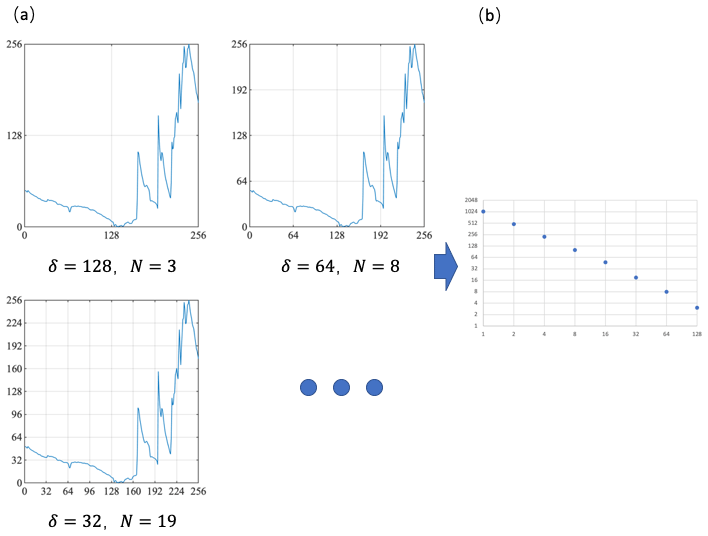
Figure 1 Flow chart for the use of the box-counting method to calculate the Hausdorff dimension of a time series.

As stated before, the observed and simulated streamflow series should have the same Hausdorff dimension. In this study, a new criterion, the ratio of fractal dimensions (RD), is defined as follows:

$$\begin{array}{}\text{(2)}& \mathrm{RD}={\displaystyle \frac{D_{\mathrm{s}}}{D_{\mathrm{o}}}},\end{array}$$

where D_s is the Hausdorff dimension of the simulated streamflow series and D_o is the Hausdorff dimension of the observed streamflow series. RD ranges from 0 to +∞. When RD=1, the simulated streamflow series has the same Hausdorff dimension as the observed streamflow series, which means that the model is the best in terms of fractals. The relevant examination of model performance under the supervision of RD is yet to be studied.

Obviously, given that RD is a metric of the deviation of the self-affinity of the simulated streamflow series from that of the observed series, it cannot be used to evaluate the performance of a hydrological model by itself. An immediate thought is to combine RD with another statistical criterion in model calibration. The statistical criterion to be combined with RD should have three features. Firstly, the statistical criterion should be able to evaluate model performance in terms of the water balance to some extent. Secondly, the statistical criterion should evaluate the response of the streamflow to meteorological forcing. Thirdly, the criterion should calculate model errors over the entire test period. These features ensure that the basic requirements of the strategy are fulfilled. An additional requirement for the statistical criterion used in this study is that it is popular within the hydrological community. Therefore, in this study, E is used as the statistical criterion. Another reason to use E is that hydrologists are more familiar with the pros and cons of E than with those of other metrics, and this original version is still commonly used in hydrological model calibration even if some variants of E have been raised. In this manner, we can obtain the advantages of RD as well as the benefits of multi-objective calibration based on RD.

The Nash–Sutcliffe efficiency coefficient (E), a criterion that has been commonly used since it was initially proposed (Nash and Sutcliffe, 1970), is calculated via

$$\begin{array}{}\text{(3)}& E=\mathrm{1}-{\displaystyle \frac{\sum {\left(Q_{\mathrm{o}}-Q_{\mathrm{s}}\right)}^{\mathrm{2}}}{\sum {\left(Q_{\mathrm{o}}-\stackrel{\mathrm{‾}}{Q_{\mathrm{o}}}\right)}^{\mathrm{2}}}},\end{array}$$

where Q_s is the simulated flow, Q_o is the observed flow and $\stackrel{\mathrm{‾}}{Q_{\mathrm{o}}}$ is the mean value of the observed flow.

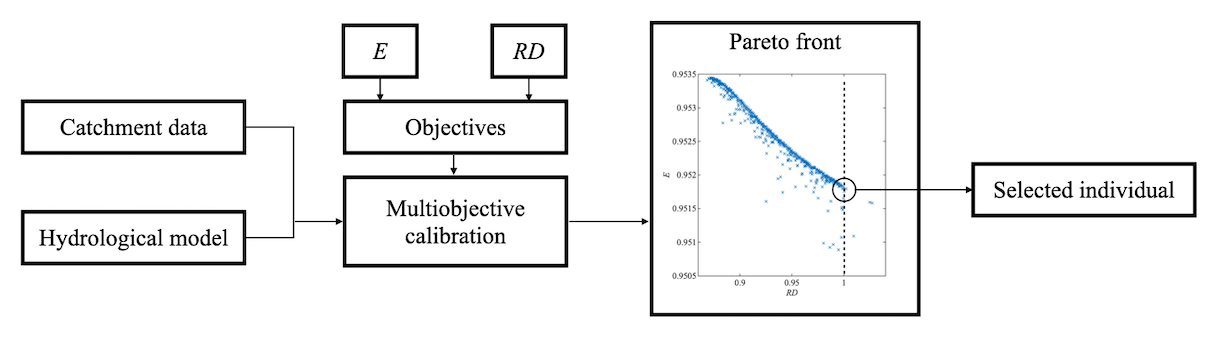
In this work, a set of experiments are performed to illustrate the benefits of using the proposed E–RD strategy to evaluate models. Descriptions of these experiments are included in Sect. 3. Figure 2 presents the complete E–RD strategy.

Figure 2 Flow chart of the E–RD strategy.

The value of the Hausdorff dimension of a particular time series may vary with the resolution applied. This implies that the self-affinity of the time series changes as the resolution changes and, for hydrological processes, the dominant driver of those processes changes. For example, the dominant drivers of the daily and annual temperature cycles are different. The Hausdorff dimension of a joint data series can be used to verify the simulation of the freezing–thawing process that reveals the complex relationship between the hydrological variables (Bai et al., 2019). According to this idea, the Hausdorff dimension determines whether the streamflow components are reasonably simulated. In the present study, the largest temporal resolution is set to 365 d (1 year) in order to eliminate interannual drivers. It is believed that the resulting resolution range is large enough for the Hausdorff dimension to accurately reflect the drivers of hydrological processes.

2.2 Study area

A small catchment in Tibet named Dong, a medium-sized catchment in southeastern China named Jinhua, and a large catchment located in the middle reach of the Yangtze River and named Xiang are examined in this study.

Dong is a small tributary of the Yarlung Zangbo River, with elevations ranging from 3512 to 5869 m. The area of the Dong catchment is about 43.6 km². The average annual precipitation in this catchment during the study period was 413.5 mm. The average temperature was 10.6 ^∘C. The high elevation of the Dong catchment results in a cold climate. A previous study found that snowpack and frozen soil significantly affect hydrological processes in the Dong catchment (Bai et al., 2019). The meteorological forcing data and streamflow observations for the Dong catchment used in this study date from 2011 to 2014.

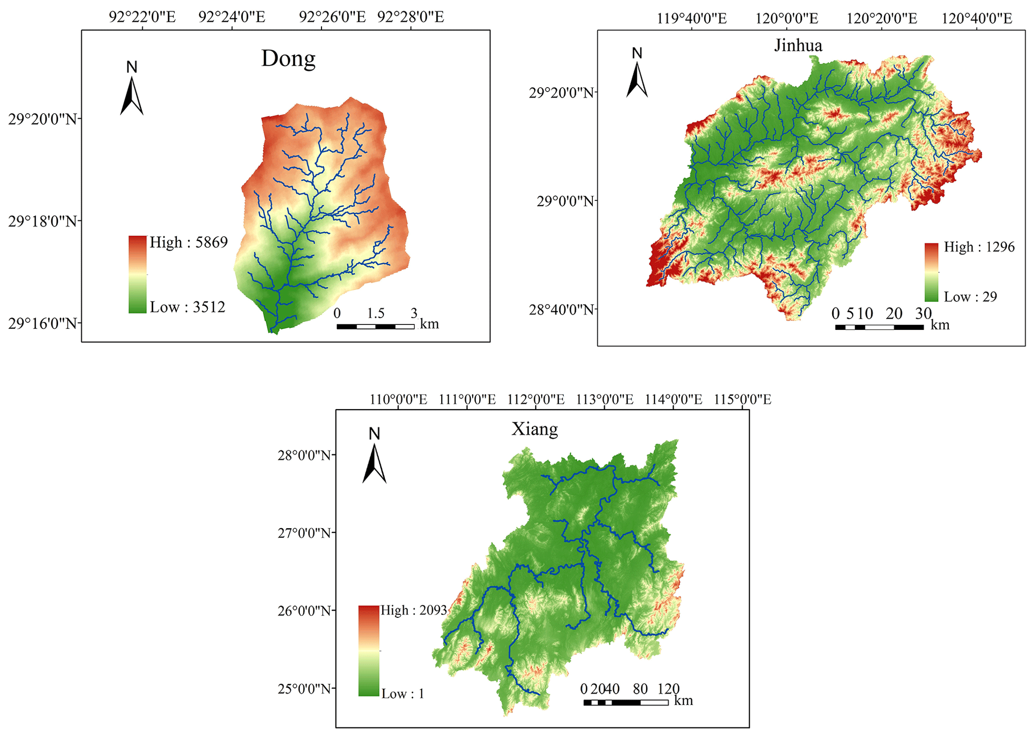
Figure 3 Digital elevation models of the study areas.

Jinhua River is a 5536 km² catchment in Zhejiang Province, southeastern China. The study area is subject to an Asian monsoon climate, and precipitation is strongly summer dominant, occurring mostly from May to September. Based on 42 years of meteorological data (from 1965 to 2006), the mean annual precipitation in the Jinhua catchment is 1847.4 mm and the average temperature is 17.6 ^∘C. Studies have shown that precipitation data and streamflow data for the Jinhua catchment are well matched (Pan et al., 2018). Meteorological forcing data and streamflow observations for the Jinhua catchment used in this study date from 1965 to 2006.

Xiang River is one of the largest tributaries of the Yangtze River, which flows into Dongting Lake, the second largest freshwater lake in mid-China. The area of the Xiang catchment is about 82 400 km², and data from nine meteorological stations are used in this study. Due to its subtropical monsoon climate, the mean annual rainfall of the basin ranges from 1400 to 1700 mm and the average annual temperature is around 17 ^∘C. The basin experiences floods and droughts frequently, and rainfall is distributed evenly throughout the year, with most of it falling in April to June. According to studies, precipitation is the main driver of the Xiang River (Zhu et al., 2019). Meteorological forcing data and streamflow observations for the Xiang catchment used in this study date from 1987 to 2013.

Figure 3 shows the topographies of all the study areas.

2.3 HBV model

The HBV model is a conceptual rainfall-runoff model originally developed by the Swedish Meteorological and Hydrological Institute (SMHI) (Bergström, 1976; Bergström, 1992; Lindström et al., 1997). This model has been successfully used in many studies (Seibert and Vis, 2012; Tian et al., 2015, 2016). The HBV model is composed of precipitation and snow accumulation routines, a soil moisture routine, a quick runoff routine, a baseflow routine and a transform function. The HBV model takes into account the effect of snow melting and accumulation, which is significant in the Dong catchment. The actual evapotranspiration is calculated with a linear function. Two conceptual runoff reservoirs – the upper reservoir and the lower reservoir – are included in the HBV model.

2.4 Multi-objective genetic algorithm

A controlled and elitist genetic algorithm (a variant of NSGA-II) (Deb, 2001) is applied in model calibration. A controlled and elitist GA favours individuals with high fitness values (ranks) as well as individuals that can help increase the diversity of the population, even if they have low fitness values. An important feature of this genetic algorithm is that the individual with the best performance according to any criterion is retained with the lowest rank. This ensures that when using a multi-objective genetic algorithm, the parameter set with the best possible E is found and the subsequent comparison between RD–E and E is reasonable. In this study, $|\mathrm{1}-\mathrm{RD}|$ is used as one of the criteria.

Since HBV has 14 parameters to calibrate, the number of generations is 2800. Each generation has a population of 600. The crossover fraction is set to 0.8 (average). The Pareto fraction is set to 0.2 (average). The population migrates every 20 generations, and the migration fraction is set to 0.5. These settings ensure that the population is not trapped in a local optimum, which is important because RD has a wider range than traditional criteria. Most of these settings are the default settings applicable to most problems. Only the population of each generation (600) is larger than the default (200) to better represent the Pareto front of the optimization. The meanings of the settings can be found in Deb (2001).

All 600 Pareto-optimized solutions for the last generation are used in the following analysis. In GA optimization with the E–RD calibration strategy (described in Sect. 2.1), populations with a perfect RD (=1) but an unsatisfactory E are retained. Several representative selected parameter sets and corresponding simulated streamflow series are studied in depth.

2.5 Approach used for model evaluation

Several tools are utilized to investigate the effects of using RD in hydrological model evaluation.

Pearson's correlation coefficient (r²), the percentage bias (bias), the autocorrelation of the observed data, the autocorrelation of the simulated data, the relative variance, the maximum monthly flow and the minimum monthly flow are used to comprehensively compare models based on RD and the hydrological criterion E. The model with the best RD and the model with the best E (typical models) are selected from the last generation obtained in GA calibration for detailed analysis.

To elucidate how the model is altered when RD is used as one of the objectives, the relationships between the parameters and RD are analysed. The distance correlation $r_{\mathrm{d}}^{\mathrm{2}}$ is used to determine whether variations in the model parameters and RD are related. The distance correlation, a multivariate measure of dependence, is calculated by determining the correlations of distances between points with means. The distance correlation is believed to provide better performance when solving problems involving nonlinear data or extreme values (Székely et al., 2007). The relationships between the parameters and RD may not be linear, which makes it necessary to use a nonlinear analysis approach rather than Pearson's linear correlation coefficient. Distance correlation is also more robust than rank correlation to data outliers.

To study the influences of specific parts of the hydrograph on the simulation when using RD, the fast flow and baseflow are analysed separately. The HBV model is slightly modified to output the simulated fast flow and baseflow at every time step. Observed streamflow series are divided into the fast flow and the baseflow using the Water Engineering Time Series PROcessing tool (WETSPRO tool) introduced by Willems (2009). WETSPRO separates the fast flow from the slow flow using filter theory with several filter parameters, including the recession constant and the the average ratio of the fast flow volume to the total flow volume. The E and r² of the simulated fast flow/baseflow with respect to the observed fast flow/baseflow are calculated. Hydrographs for the first 3 years after warming up are shown to visually illustrate the influence of RD on fast flow and baseflow simulation.

3 Results and discussion

3.1 Overall evaluation of models on the Pareto front

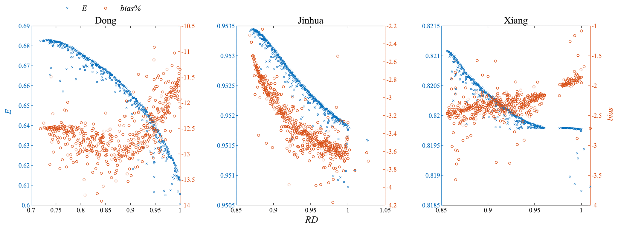
Figure 4 shows the RD–E relationship of the last population from multi-objective calibration for each of the three catchments. The RD range of the final generation differs for the three cases, as does the range of E/bias. The range of E is 0.60–0.69 for the Dong catchment, 0.95–0.953 for the Jinhua catchment and 0.818–0.822 for the Xiang catchment. In all three cases, the nonsignificant variation of E indicates that for all selected parameter sets, the E criterion could not fully distinguish the selected parameter sets. The ranges of RD are about 0.72–1 (Dong), 0.86–1.04 (Jinhua) and 0.85–1.01 (Xiang). According to relevant studies, the biggest difference in Hausdorff dimension for data of the same type is smaller than 0.25 (Hurst, 1951; Rubalcaba, 1997; Meseguer-Ruiz et al., 2019), which indicates that the aforementioned ranges of RD represent significant differences in simulated streamflow from the fractal perspective. In this study, RD is often lower than 1 and sometimes slightly higher than 1, which agrees with the smooth hydrograph and the simple structure of the HBV model. Because a model with RD=1 is best from the fractal perspective (see Sect. 2.2), we should also discuss models with RDs that are larger than 1. Since the largest RD is very close to the best RD (=1), the largest-RD model should be similar to the best-RD model. The GA algorithm discards most of the models with RD>1 because they are not on the Pareto front. The bias does not change much when RD changes. A tiny difference (within 3 %) occurs for the last generations from GA calibration for Dong, Jinhua and Xiang. More importantly, the change in bias as a function of RD is different for the three cases. For the Dong catchment, the bias first worsens but then improves as RD approaches 1. On the other hand, the bias worsens for Jinhua and improves for Xiang as RD approaches 1. Based on these cases, the bias seems to vary randomly as a function of RD. In addition, there is a break in the data for the Xiang catchment in Fig. 4. The values of E are similar but the values of RD are significantly different on both sides of the break.

Figure 4 E–RD plots for the last generation from GA calibration.

A single-objective calibration was performed to support an assumption made in Sect. 3.3: that, in this work, the NSGA II algorithm can find the best E. A comparison between the results of single-objective calibration and the results of multi-objective calibration (E–RD strategy) is provided in Table 1. Also, to get rid of any possible influence of the length of the time series, the results of multi-objective calibration for different time-series lengths were compared. The results showed that, at least in the cases examined in this study, the E–RD strategy does not change its behaviour with time-series length.

Table 1 Comparison of the best E values obtained with single-objective calibration and multi-objective calibration (E–RD strategy).

The models in the Pareto front with the best RD, best E and largest RD values were selected as typical examples. Figure 5 shows the simulated streamflows of those three examples, as well as the observed streamflow, for each catchment. For each case, the discharge within a 3 year period is shown. The examples with the largest RD values were used to verify that the model with RD = 1 is the best. The simulated hydrographs of the typical models in each case appear to be similar, which agrees with the E and RD results shown in Fig. 4.

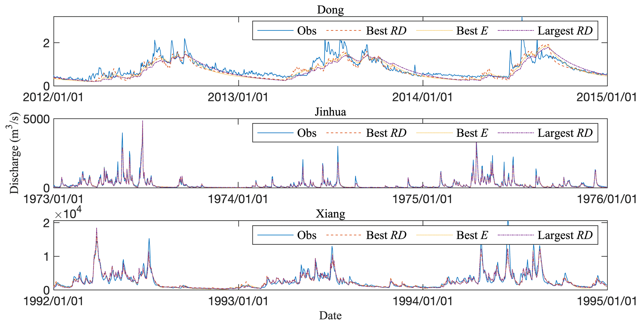
Figure 5 Typical examples of models: those with the best RD, the best E and the largest RD (representative 3 year hydrographs are shown).

A precondition for adopting the RD–E strategy is that the correlation between the two criteria is irrelevant or weak. This precondition can be verified by simply looking at their calculation schemes or by examining the results of the multi-objective calibration. In this study, the two metrics (RD and E) are calculated in totally different ways, and the results of multi-objective calibration also show that significantly changing RD leads to only a minor change in E (see Fig. 4). The best E is close to the worst E according to the results of multi-objective calibration. Figures 4 and 5 also imply that pursuing a better RD leads to only a minor decrease in E. This study demonstrates the equifinality of using only E.

Table 2 lists hydrological signatures of typical models selected by the E–RD calibration strategy. Table 2 confirms the assumption that, in this study, directly analysing the models calibrated using the E–RD calibration strategy is reasonable and efficient. Hydrological signatures including the relative variance, lag-1 autocorrelation, percentage bias and maximum/minimum monthly flow are used to show the effect of RD.

Table 2 Hydrological signatures of the typical models in all three cases.

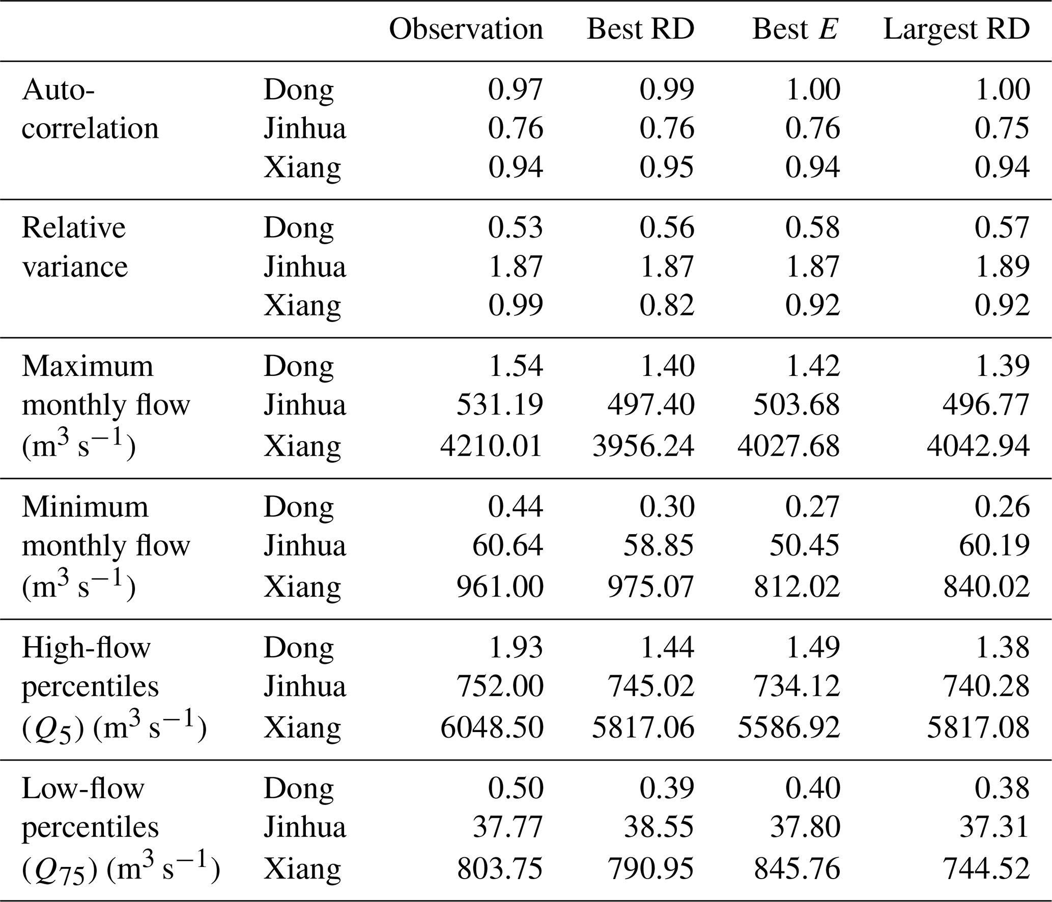
Table 2 shows the hydrological signatures of the observed and simulated flow series in the three cases. Most of the hydrological signatures, including the lag-1 autocorrelation, relative variation and maximum monthly flow, of the simulated series are close. The lag-1 autocorrelations of the simulated series are similar to the autocorrelations of the observed flow series. The lag-1 autocorrelations for the Dong and Xiang flow series are more than 0.9 while those for the Jinhua series are between 0.75 and 0.77. The relative variances of the flow series for the Dong and Xiang catchments are smaller than 1, while those for the Jinhua flow series are more than 1.8. These results show that catchments of different types are well simulated by the HBV model. The maximum and minimum monthly flows of the simulated and observed series are significantly different. In all three cases, the maximum monthly flows of the simulated series are similar to each other and slightly smaller than the maximum monthly flows of the observed flow series. The minimum monthly flow is the only hydrological signature used in this study that identifies the models with the best RD and the best E. In all three cases, the minimum monthly flow of the simulated series with the best E is significantly smaller than the minimum monthly flow of the observed series. On the other hand, the minimum monthly flow of the simulated series with the best RD is close to the minimum monthly flow of the observed series for Jinhua and Xiang. The minimum monthly flow of the simulated series with the largest RD is worse than that of the simulated series with the best RD. The high-flow percentiles (Q₅) and the low-flow percentiles (Q₇₅) are reasonable for all the typical models in all three cases. However, the high-flow percentiles and low-flow percentiles of the best-RD models are still closest to those of the observed series. In summary, the hydrological signatures illustrate that RD has the greatest effect on the simulation of low flow by the models. Therefore, in subsequent sections, low-flow-related analysis is emphasized.

3.2 Effect of RD on model parameters

The parameter set in the Pareto front varies depending on the case considered. The distance correlations ($r_{\mathrm{d}}^{\mathrm{2}}$) of the parameters with RD are used to determine whether a change of parameters is stable. In addition, a high value of $r_{\mathrm{d}}^{\mathrm{2}}$ indicates a significant relationship between the Hausdorff dimension and the parameter considered. In this study, the relation between GA-selected parameter sets and E is not shown because E and RD are strongly related in the Pareto front and the variance of E is small (see Fig. 4).

Table 3 Ranges of the determinative parameters and distance correlations ($r_{\mathrm{d}}^{\mathrm{2}}$) between those parameters and RD. ^* $r_{\mathrm{d}}^{\mathrm{2}}\ge \mathrm{0.8}$.

Figure 6 Relationship between β and RD in the three cases.

Figure 7 Relationship between α and RD in the three cases.

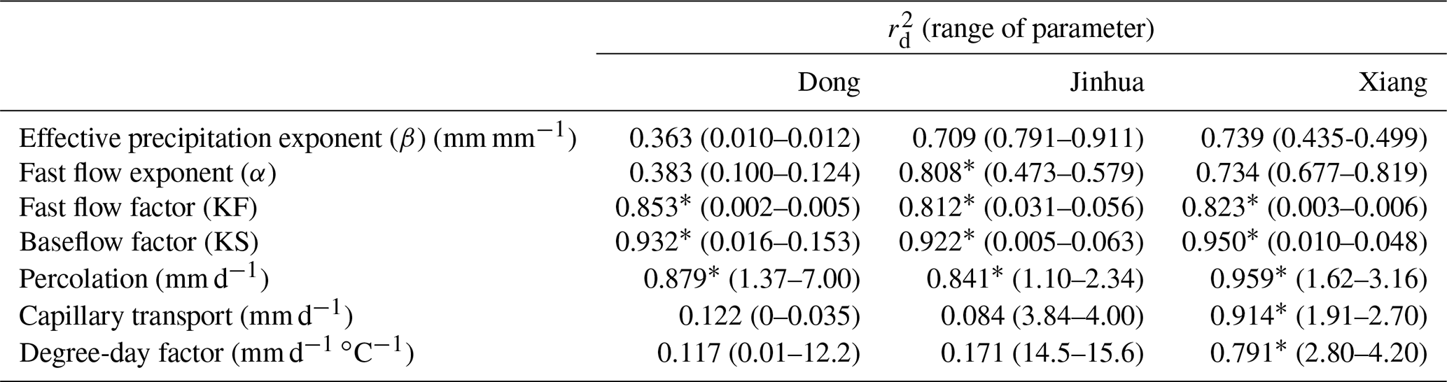
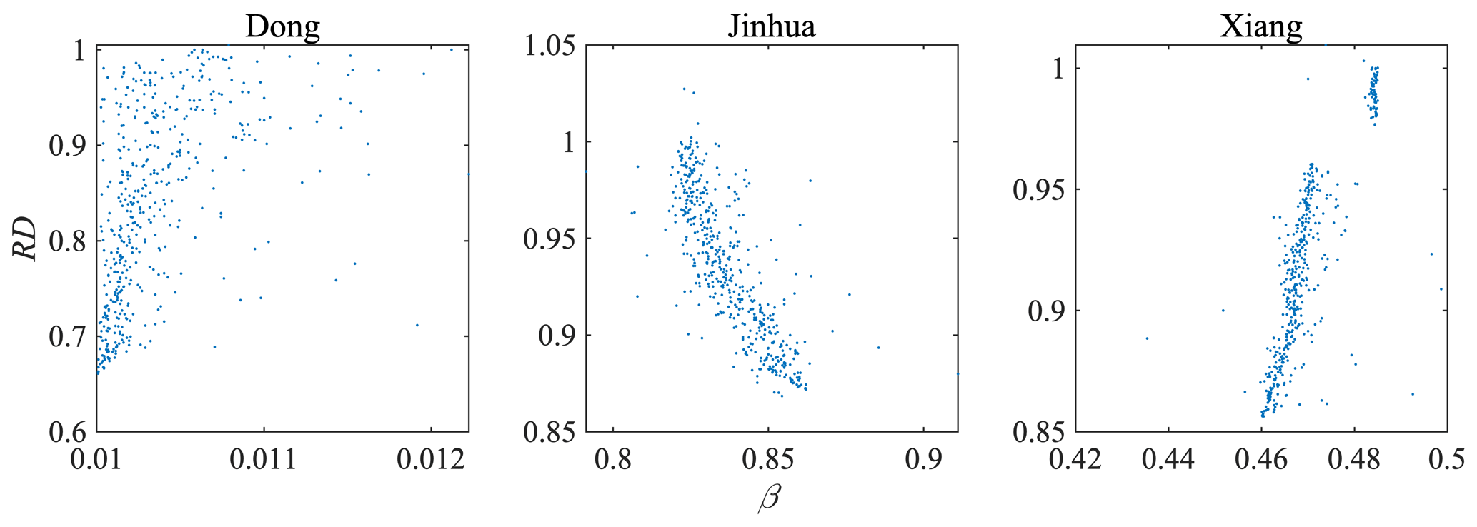
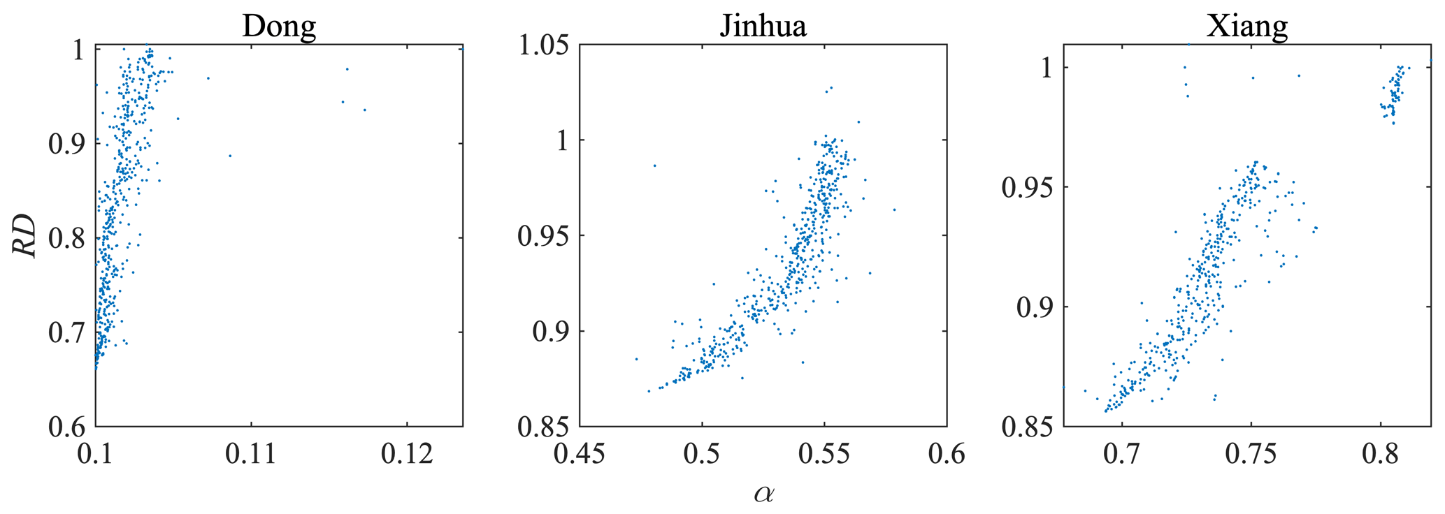
Table 3 lists the determinative parameters for the three cases. The distance correlation ($r_{\mathrm{d}}^{\mathrm{2}}$) is used to illustrate the nonlinear relationship between E and RD in the Pareto fronts. The effective precipitation exponent (β) and the degree-day factor are also listed in Table 3. The effective precipitation exponent is listed in Table 3 for two reasons. First, the $r_{\mathrm{d}}^{\mathrm{2}}$ of β is 0.709 for Jinhua and 0.739 for Xiang, which are better than the $r_{\mathrm{d}}^{\mathrm{2}}$ values of all the unlisted parameters. Second, β is a runoff-generation-related parameter, as are the determinative parameters α, KF and KS. The degree-day factor is listed in Table 3 for two reasons. First, the distance correlation between the degree-day factor and RD is close to 0.8 for Xiang. Second, for Dong, distance correlation analysis does not reflect the significance of snow ablation to the hydrograph. Capillary transport is not a determinative parameter of RD for Dong and Jinhua, so they are not discussed further here. The $r_{\mathrm{d}}^{\mathrm{2}}$ of β (0.512) in the Dong catchment is smaller than those for the other two cases. Figure 6 shows the relationship between β and RD.

The explicit relationship between the parameters and the criteria confirms that the effect of RD is not random. Six parameters (β, α, fast flow factor, baseflow factor, percolation and degree-day factor) were selected for further discussion based on the distance correlation analysis.

Figure 7 shows the relationship between α and RD. The fast flow factor (KF) is related to RD in all cases. Figure 8 shows the relationship between KF and RD. The trends in α and KF are the same in all three cases. The fast flow exponent α increases as RD approaches 1 and KF decreases as RD approaches 1.

Figure 8 Relationship between KF and RD in the three cases.

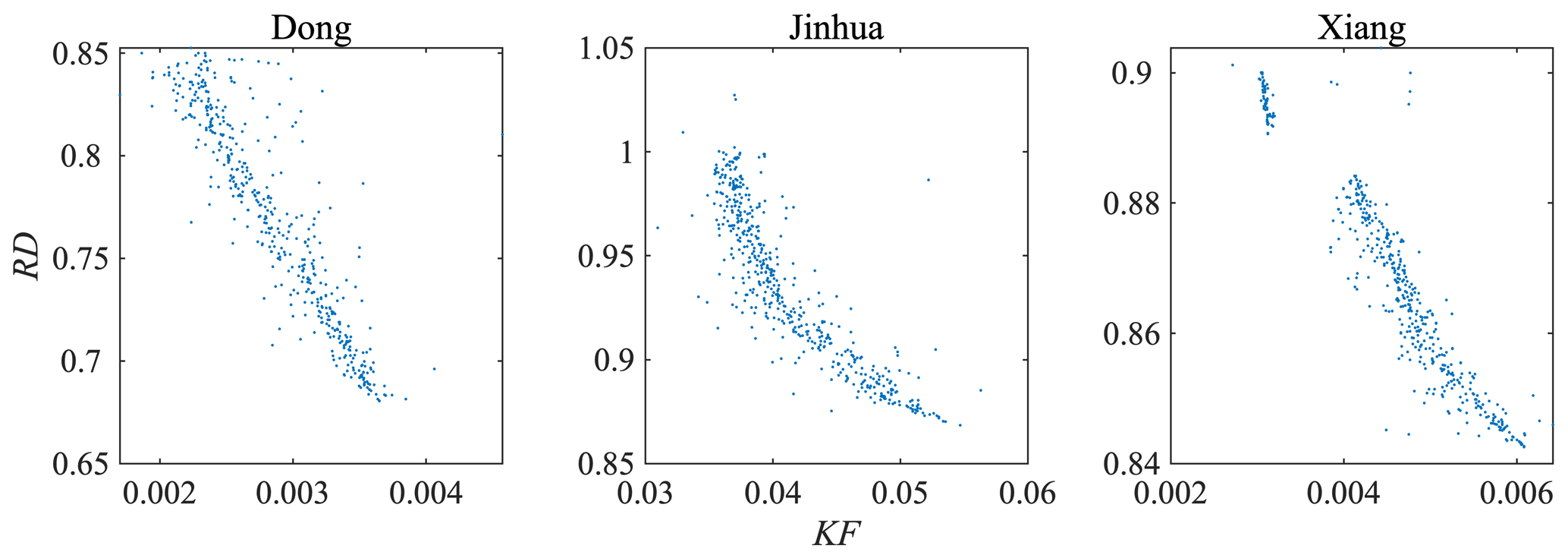
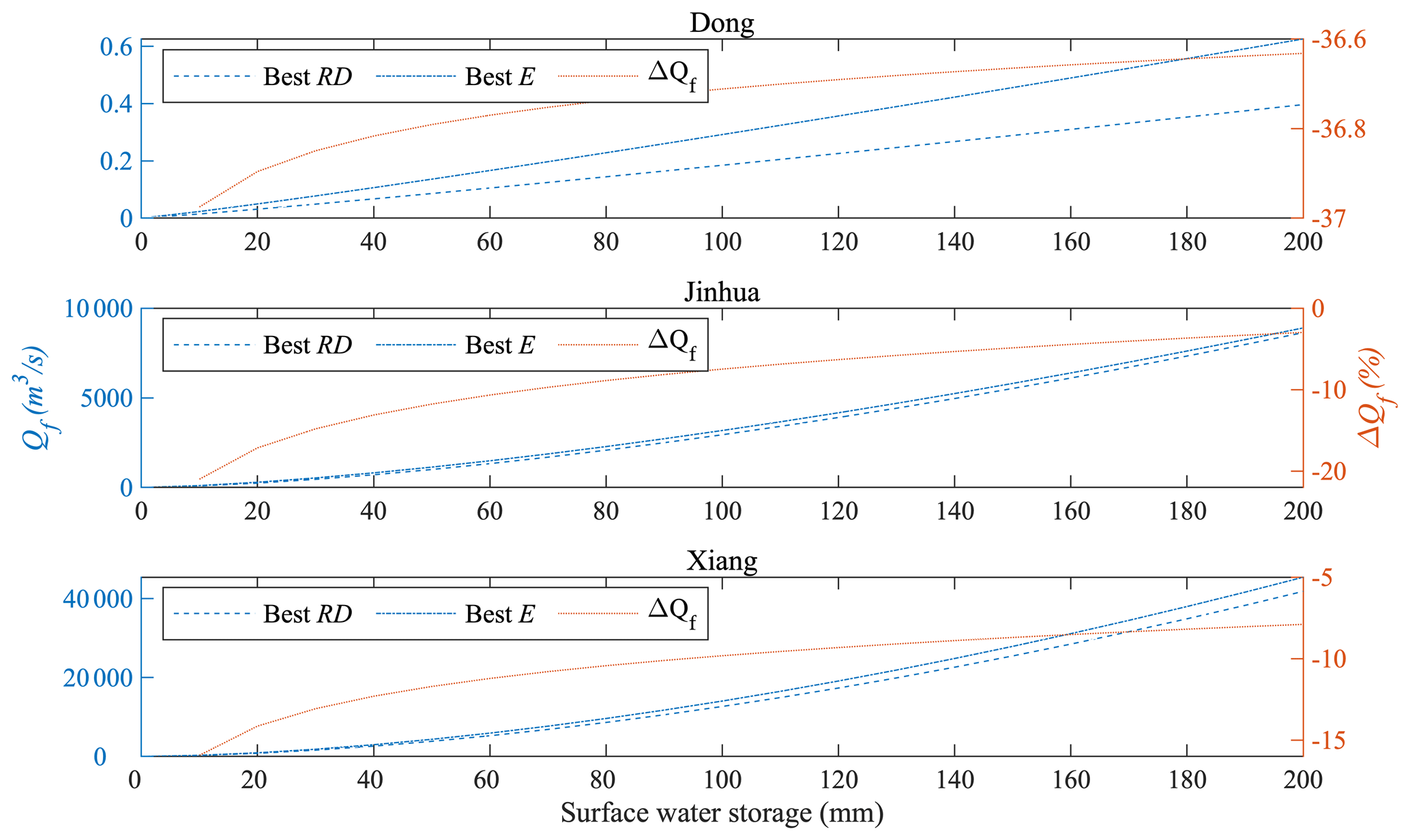
Figure 9 Response of fast flow to surface water storage. For each case, the fast flow responses of the typical models with the best RD and E are presented.

Figure 9 shows how the fast flow changes with the surface water storage with different KF and α values in the typical models with the best RD and best E. In all cases, E selects higher KF and lower α values. For Dong, the relative difference in fast flow generation between the best-RD model and the best-E model is always around 36 %. The difference in fast flow between these two models is significant for Dong across the whole simulated period. For Jinhua, the relative difference between the best-RD model and the best-E model decreases from more than 20 % to less than 5 %. For Xiang, the relative difference between the best-RD model and the best-E model decreases from about 16 % to 8 %. The difference between the best-RD model and the best-E model is substantial during the dry period but reduces as the water stored in the upper reservoir increases (the wet period). The relative difference is greater for Jinhua than for Xiang during low-flow periods but smaller for Jinhua during high-flow periods. That difference between the best-E model and the best-RD model ultimately leads to more variation in fast flow during low-flow periods than during high-flow periods. There are break points in the case of Xiang (Figs. 6–8), but there are no evident effects in Figs. 5 and 9.

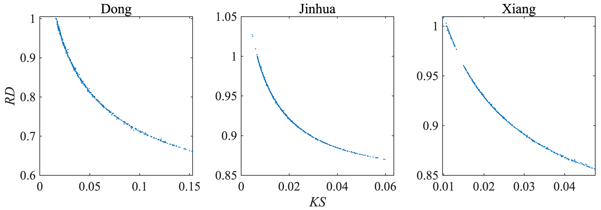
The baseflow (slow flow) factor (KS) is related to RD in all cases. Figure 10 shows the relationship between KS and RD. The trend in KS is the same in all three cases. However, the range of variation in KS is different for the three cases. The largest value of KS in Dong (0.153) is much larger than that in Jinhua (0.063) and Xiang (0.048). The smallest value of KS in Dong (0.016) is also larger than that in Jinhua (0.005) and in Xiang (0.010). The KS of the best E increases with increasing catchment areas. This agrees with the regular pattern that the generation time of slow flow is highly related to the area of the catchment.

Figure 10 Relationship between KS and RD in the three cases.

Figure 11 Relationship between percolation and RD in the three cases.

Figure 12 Relationship between degree-day factor and RD in the three cases.

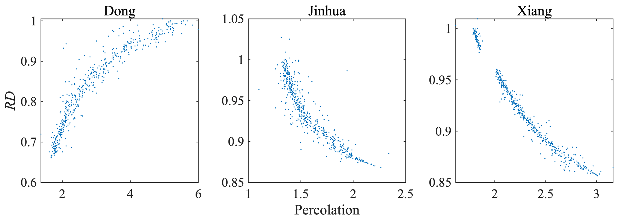
The percolation is significantly related to RD in all cases. The range of percolation in Dong is larger than in the other cases. Figure 11 shows the relationship between percolation and RD in each of the three cases. Percolation increases in Dong and decreases in the other two cases with increasing RD. The KS and percolation determine the way that HBV models the baseflow. The percolation in Dong is larger than in the other cases, which is a reflection of the arid climate of the Dong catchment. The percolation is larger in Jinhua than in Xiang because the slope in the Jinhua catchment is larger.

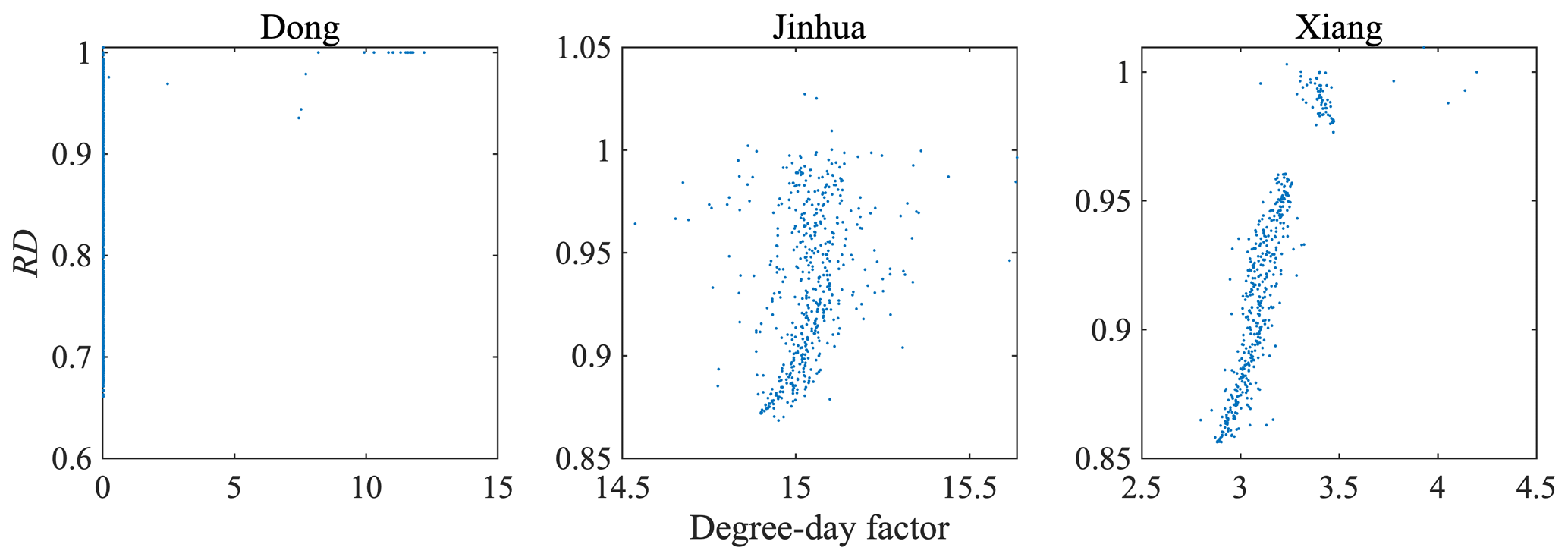
The degree-day factor is significantly related to RD in Xiang. However, the relationship between the degree-day factor and RD is weak in Dong and Jinhua. Figure 12 shows the relationship between the degree-day factor and RD in each catchment. The degree-day factor is smaller than 0.05 for most of the models selected for Dong, indicating that these models barely have any snowmelt runoff. When RD>0.9, several models have degree-day factors larger than 7. When RD is around 1, the range of the degree-day factor is 8.18–11.76, indicating that RD somehow detects the snowmelt runoff in the hydrograph and causes the HBV model to simulate the snowmelt runoff more reasonably. Note that the RD-selected degree-day factor for Dong is too large according to the HBV guide (the user manual for HBV light version 2 suggests that the factor should be 1.5–4 mm d⁻¹ in Sweden). This may be due to the lumped model structure of HBV, which is unsuitable for a rugged mountainous catchment.

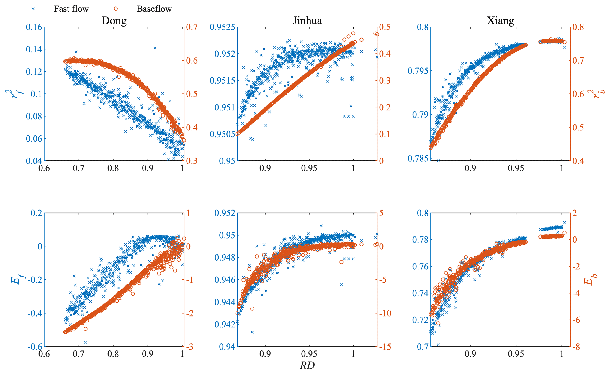
Figure 13 Correlation coefficients and Nash–Sutcliffe efficiency coefficients for fast flow and baseflow, respectively, in last-generation models for the three cases.

The degree-day factors in all the models selected for Jinhua are large, but the temperature in Jinhua is too high for snow to accumulate. The distance correlation between the degree-day factor and RD is weak for Dong and Jinhua. The range of the degree-day factor for most of the models for Xiang is 2.8–3.4. This range is small, meaning that the difference in snowmelt runoff between the selected models is too. Upon checking the temperature series for the Xiang catchment, we found that there were 61 d when the average temperature was below 0 ^∘C in 27 years. However, because the Xiang catchment is large, there are snow events somewhere in the catchment almost every year. Those low temperatures may be obscured by averaging, but the E–RD strategy captured them and reflected them in the notable value of the degree-day factor.

As illustrated in Figs. 7, 8, and 10, the three runoff-generation-routine parameters, namely the baseflow factor (KS), the fast flow factor (KF) and the fast flow exponent (α), have the same trends in all three cases, suggesting a consistent advantage of using RD. Figure 9 visualizes the difference in fast flow caused by introducing RD. However, other parameters show different trends with RD because the catchments have different features (Figs. 6 and 12). For example, the soil parameter β redistributes the precipitation and divides it into effective precipitation and infiltration. β increases in Dong and Xiang but decreases in Jinhua as RD improves.

Table 4 Parameters of WETSPRO.

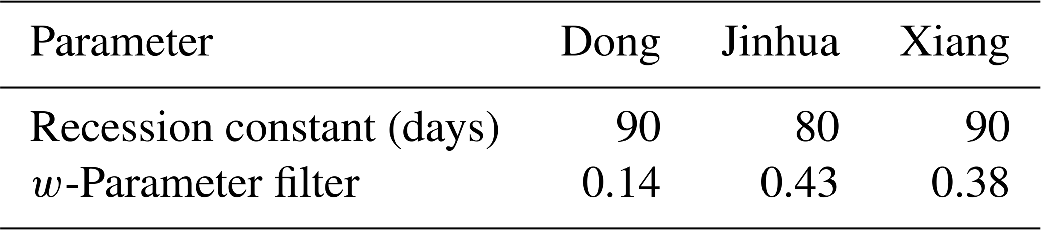
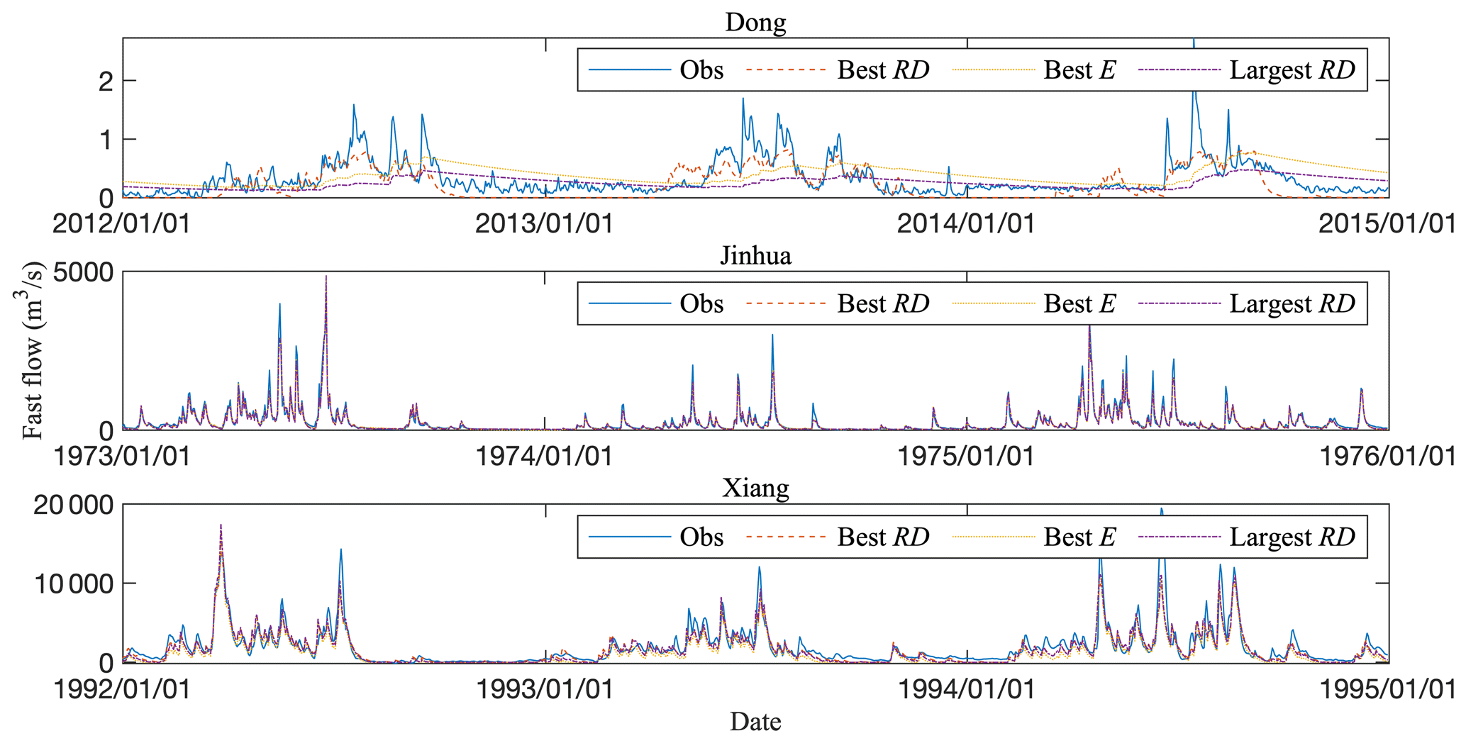
Figure 14 Fast flow in typical models and observations (representative 3 year hydrographs are shown).

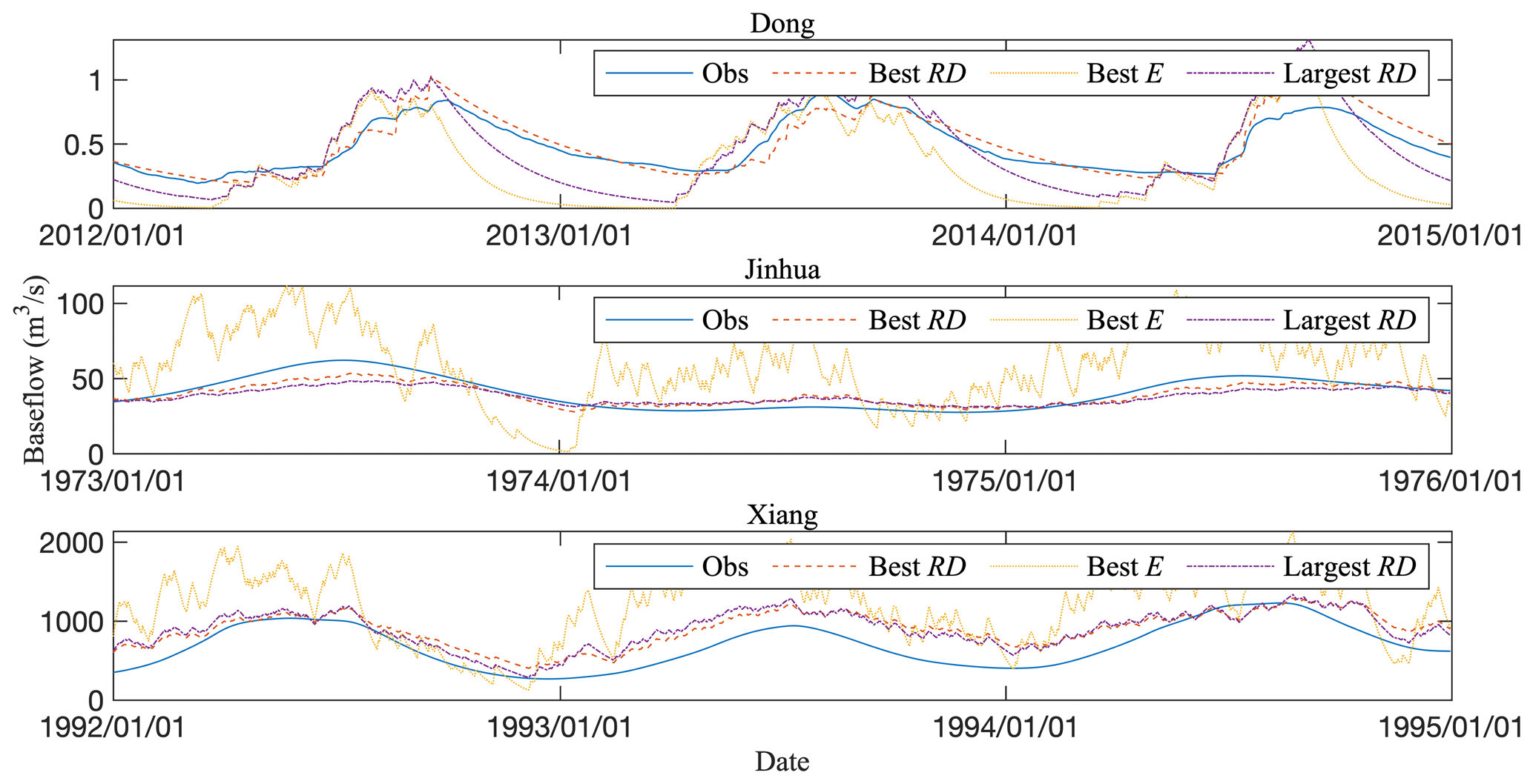
Figure 15 Baseflow in typical models and observations (representative 3 year hydrographs are shown).

3.3 Analysis of the separated streamflows

Separating both the simulated and the observed streamflow series further reveals how RD influences the model calibration results. The simulated total flow was separated with the WETSPRO tool to ensure that the same separation principle was used for the simulations and observations. Table 4 lists the parameters of WETSPRO for the three cases. The recession constants for the three cases are similar to each other. However, the w-parameter filter, which represents the case-specific average fraction of the quick flow volume with respect to the total flow volume, differs depending on the case considered. The w-parameter filter of the Dong catchment is 0.14, which is smaller than those for the other catchments, meaning that the baseflow contributes less of the total flow in Dong, reflecting the small area and high slope of this catchment. Figure 13 shows the variation in the correlation coefficient between the simulated and observed fast flow or baseflow ($r_{\mathrm{f}}^{\mathrm{2}}$ and $r_{\mathrm{b}}^{\mathrm{2}}$, respectively) with RD and the variation in the Nash–Sutcliffe efficiency coefficient for fast flow or baseflow (E_f and E_b, respectively) with RD for the complete population of the last generation in each case. The observed fast flow and baseflow were separated from the observed total flow using WETSPRO (Willems, 2009) (see Sect. 3.4). For Dong, both $r_{\mathrm{b}}^{\mathrm{2}}$ and $r_{\mathrm{f}}^{\mathrm{2}}$ decrease slightly as RD approaches 1. However, $r_{\mathrm{f}}^{\mathrm{2}}$ ranges from 0.02 to 0.15 and $r_{\mathrm{b}}^{\mathrm{2}}$ ranges from about 0.3 to 0.6 for Dong, which means that there is no correlation between the simulated and observed fast flow or between the simulated and observed baseflow. Also for Dong, E_f and E_b improve to 0.06 and 0.24, respectively. All models of the last generation of GA for Jinhua and Xiang simulate the fast flow well. $r_{\mathrm{f}}^{\mathrm{2}}$ and E_f are above 0.95 and 0.94, respectively, for Jinhua. For Xiang, $r_{\mathrm{f}}^{\mathrm{2}}$ and E_f are above 0.78 and 0.70, respectively. Surprisingly, the application of RD causes an evident improvement in fast flow simulation. There is also a major improvement in baseflow simulation performance. The values of the criteria for baseflow simulation ($r_{\mathrm{b}}^{\mathrm{2}}$ and E_b) are improved from poor to satisfactory. In the case of Jinhua, $r_{\mathrm{b}}^{\mathrm{2}}$ improves from less than 0.1 to more than 0.45 and E_b improves from −10 to about 0.38. For Xiang, $r_{\mathrm{b}}^{\mathrm{2}}$ improves from about 0.4 to 0.75 and E_b improves from −6 to 0.51.

Figures 14 and 15 show the separated streamflows of typical models and the separated observed streamflow, allowing a visual comparison of models based on E and models based on RD. Figure 14 shows the fast flow and Fig. 15 shows the baseflow.

The fast flow response of the best-RD model in Dong matches well with the observed fast flow. The recession of the fast flow in the best-RD model for Dong is too fast and the stable value is nearly zero, which contrasts with observations. The fast flow response of the best-E model for Dong is late, the recession of the fast flow is too slow, and there is too much fast flow during recession periods. The fast flow response of the largest-RD model for Dong is also late, but the fast flow recession is more reasonable. For Jinhua and Xiang, the simulated fast flows of all typical models closely match the corresponding observations. In all cases, the fast flow of the best-RD model is smaller than that of best-E model and the difference is greatest during low-flow periods, which is consistent with Fig. 9.

In all three cases, the best-RD models simulate the baseflow well. RD-selected models accurately simulate the seasonal flow variations in the three catchments. The amplitude of the baseflow fluctuation is close to that seen in the observed baseflow separated by WETSPRO. The discharge also fits with the observed baseflow well. However, in all three cases, the best-E models do not simulate the baseflow well enough. The largest-RD model varies in performance depending on the case considered. The largest-RD model for Dong (with $r_{\mathrm{b}}^{\mathrm{2}}=\mathrm{0.82}$ and E_b=0.25) is not satisfactory. In contrast, the $r_{\mathrm{b}}^{\mathrm{2}}$ and E_b of the best-E model for Dong are 0.87 and 0.79, respectively. The best-E models for Jinhua and Xiang are, however, similar to the best-RD models for those catchments. According to Figs. 10 and 11, the small KS and percolation values in the best-RD models for Jinhua and Xiang lead to small recharge and outflow (baseflow) values for the lower reservoir and smaller fluctuations in the baseflow. In Dong, high percolation increases the recharge and total baseflow, and the small KS lengthens the baseflow recession period, making the simulated baseflow more consistent with observations (Fig. 15).

There are two reasons for the unsatisfactory simulation of the fast flow in Dong. The first is that the HBV model is not capable of accurately simulating a mountainous catchment with snowpack, and gauge data for the Dong catchment are scarce. The second is that WETSPRO may have failed to correctly separate the short streamflow series of the Dong catchment. This needs to be further verified.

Further visual demonstrations of the advantage of using RD are provided by Figs. 14 and 15. Fast-flow generation based on RD is more immediate, whereas baseflow generation based on RD is smoother. Both of these are clearly better than the flows generated when RD is not taken into account.

The above results reveal the benefits of using RD and a slight decrease in E. The following selection principle based on multi-objective calibration is therefore suggested: (1) sieve out all parameter sets for which the RD is around 1 (in this case, considering the data precision of MATLAB, RD=1) and (2) choose the remaining parameter set with the best E. Applying the E–RD strategy using this selection principle is found to improve the reliability of streamflow component simulation. That is, RD selects the responsive fast flow (as confirmed by Fig. 14) and the smooth baseflow (as confirmed by Fig. 15) in all cases.

4 Conclusion

This study aimed to examine the possibility of using fractal theory to improve the performance of hydrological models. The ratio of fractal dimensions (RD) was defined and proposed as a fractal criterion (rather than traditional statistical criteria). A scheme that used a combination of RD and the Nash–Sutcliffe efficiency coefficient (E) to calibrate hydrological models was developed and examined. Three study cases relating to the Dong, Jinhua and Xiang catchments were included in the examination. This is the first time (to the best of our knowledge) that fractal theory has been applied to calibrate hydrological models.

The main conclusions of this study are as follows:

1. The trends in the runoff generation routine parameters (namely the fast flow factor, fast flow exponent and baseflow factor) were similar in all three cases studied.

2. Several parameters were found to be related to RD. For instance, the E–RD strategy selected relatively high degree-day factors for Dong, which did not occur when only E was considered.

3. The E–RD calibration strategy is an innovative approach to hydrological modelling; it potentially provides a way to take the fractality of an observed streamflow series into consideration in model calibration. Since fractals (also termed self-affinity) widely exist in nature, the introduction of RD as a criterion could be a good addition to hydrological model calibration.

More case studies are needed to further corroborate the applicability of the E–RD strategy introduced in this study. The combination of other traditional statistical criteria with RD should also be examined. More studies are also needed to identify other benefits of applying fractal theory in hydrological modelling.