Statistical modelling and climate variability of compound surge and precipitation events in a managed water system: a case study in the Netherlands

The co-occurrence of (not necessarily extreme) precipitation and surge can lead to extreme inland water levels in coastal areas. In a previous work the positive dependence between the two meteorological drivers was demonstrated in a managed water system in the Netherlands by empirically investigating an 800-year time series of water levels, which were simulated via a physical-based hydrological model driven by a regional climate model large ensemble.

In this study, we present an impact-focused multivariate statistical framework to model the dependence between these flooding drivers and the resulting return periods of inland water levels. This framework is applied to the same managed water system using the aforementioned large ensemble. Composite analysis is used to guide the selection of suitable predictors and to obtain an impact function that optimally describes the relationship between high inland water levels (the impact) and the explanatory predictors. This is complex due to the high degree of human management affecting the dynamics of the water level. Training the impact function with subsets of data uniformly distributed along the range of water levels plays a major role in obtaining an unbiased performance.

The dependence structure between the defined predictors is modelled using two- and three-dimensional copulas. These are used to generate paired synthetic precipitation and surge events, transformed into inland water levels via the impact function. The compounding effects of surge and precipitation and the return water level estimates fairly well reproduce the earlier results from the empirical analysis of the same regional climate model ensemble. Regarding the return levels, this is quantified by a root-mean-square deviation of 0.02 m. The proposed framework is able to produce robust estimates of compound extreme water levels for a highly managed hydrological system. Even though the framework has only been applied and validated in one study area, it shows great potential to be transferred to other areas.

In addition, we present a unique assessment of the uncertainty when using only 50 years of data (what is typically available from observations). Training the impact function with short records leads to a general underestimation of the return levels as water level extremes are not well sampled. Also, the marginal distributions of the 50-year time series of the surge show high variability. Moreover, compounding effects tend to be underestimated when using 50-year slices to estimate the dependence pattern between predictors. Overall, the internal variability of the climate system is identified as a major source of uncertainty in the multivariate statistical model.

1 Introduction

Floods, wildfires, and heatwaves typically result from the combination of several physical processes (e.g. Baldwin et al., 2019; Manning et al., 2019; AghaKouchak et al., 2020). The physical drivers of such processes are not necessarily extreme or hazardous when occurring in isolation, but they can lead to significant impacts when occurring altogether, or in a narrow time range (Seneviratne et al., 2012). Extreme events resulting from the combinations of physical drivers are referred to as compound events, and they can be classified into different (not entirely exclusive) categories (Zscheischler et al., 2020). These compound climate extremes are receiving increasing attention because of their disproportionate economic, societal, and environmental impacts, and because traditional univariate approaches can lead to strongly biased estimates of the associated risks (Wahl et al., 2015). However, many challenges still lay ahead in order to properly understand (and predict) the complex chain of drivers that leads to compound events. Estimating the dependencies among drivers is challenging mainly due to the limited amount of data available, especially for rare events (Zscheischler et al., 2018). Moreover, the definition of multivariate extremes is not as straightforward as in the univariate case. A paradigm shift from a classical top-down approach adopted in many climate studies towards an impact-centric perspective is needed (Zscheischler et al., 2018).

Compound flooding in coastal settings often originates from a combination of storm-driven waves and surges and blocked discharge of terrestrial water from, for example, intense precipitation or snowmelt. Meteorological conditions can lead to a (nearly) simultaneous occurrence of storm surge or waves and a discharge peak when the area that generates the discharge is located close to the coast. These types of events have the potential to occur in many coastal regions across the globe (Ward et al., 2018; Couasnon et al., 2020). Low-lying coastal regions are particularly susceptible to flooding caused by the interaction of different hazards (i.e. compound flooding), including oceanographic, pluvial, and/or fluvial hazards (Hendry et al., 2019). Thus, the assessment of multivariate events has received increasing attention in the coastal engineering and management communities (e.g. Anderson et al., 2019; Serafin and Ruggiero, 2014; Rueda et al., 2016; Wahl et al., 2015). The associated impacts strongly depend on the catchment features and the characteristics of the storms (Wahl et al., 2015). For discharge peaks originating from remote precipitation or snowmelt inputs (for instance in larger river systems), delays between the surge and discharge peaks are usually due to the finite travel speed of the discharge wave (Khanal et al., 2019b; Klerk et al., 2015).

With the aim to obtain methods computationally less expensive than numerical simulations, statistical models have been used to model compound events and estimate their probability of occurrence. In some specific cases, bi- or multivariate distributions can be derived directly from physical properties (e.g. the joint distribution between wave height and wave periods in wind-sea states as a function of wave steepness; de Waal and van Gelder, 2005). However, these are often limited to idealized or very specific settings and rely heavily on the selection of the marginal distributions. In contrast, copula-based methods (Sklar, 1959) have the advantage to capture the dependence between a set of variables independently from their marginal distributions (Genest and Favre, 2007), which explains why they have become a widely used approach nowadays. In recent years, several copula-based studies have been carried out to study compound flooding events in coastal areas at different spatial scales (e.g. Couasnon et al., 2018; Moftakhari et al., 2019; Jane et al., 2020). For example, Bevacqua et al. (2017) developed and implemented a conceptual statistical model to quantify the risk of compound floods that result from the combination of storm surge and high river runoff in Ravenna (Italy). At regional scale, Wahl et al. (2015) assessed the historical changes in the compound flooding due to precipitation and storm surge in US cities and identified a significant increase in the number of compound events over the past century in major coastal cities. Accounting for climate change projections, Bevacqua et al. (2019) showed how global warming can increase the probability of compound coastal flooding in northern Europe. At a global scale, Couasnon et al. (2020) provided a perspective of the compound flood potential from riverine and coastal flood drivers, which highlighted the complexity and large regional variability of such dependence structures. Dependence between ocean wave heights and storm surges was recently investigated by Marcos et al. (2019) at the global scale, showing that 55 % of the world's coastlines face compound storm surge wave extremes.

This study is motivated by a near-flooding event in 2012 in the Lauwersmeer reservoir in the Netherlands that was classified as a compound event (van den Hurk et al., 2015). This multivariate event was characterized by a high inland (reservoir) water level (IWL) exceeding predefined warning levels and resulted from the joint occurrence of heavy precipitation on an already wet soil and a high storm surge impeding gravitational drainage over several consecutive tidal periods. In terms of the categorization of Zscheischler et al. (2020), this event can be classified as a multivariate, preconditioned, and temporally compounding event, which illustrates the complexity of this near-flooding event. The study by van den Hurk et al. (2015) empirically assessed the return periods associated with compound extreme water levels with a single model initial-condition large ensemble (SMILE) of regional climate model (RCM) simulations covering 800 years under present-day climate conditions. Using SMILEs is a physically based approach to increase the size of the database and therefore increase the number of simulated extreme compound events. Apart from van den Hurk et al. (2015), SMILEs have been applied as a tool to investigate compound events by, for example, Zhou and Liu (2018), Khanal et al. (2019a), and Poschlod et al. (2020). This methodology allowed van den Hurk et al. (2015) to demonstrate a positive dependence between storm surge and heavy precipitation and showed that the probability of occurrence of these extreme water levels can be greatly underestimated if such dependence is omitted.

Here, we develop a copula-based statistical framework to model the extreme water levels in the Lauwersmeer reservoir, including the dependence among the underlying drivers. Using the same aforementioned 800-year climate ensemble, we reproduce the results empirically obtained by van den Hurk et al. (2015) and provide additional insights into the underlying physical factors and modelling uncertainties in compound analysis. Although the study is site specific, we address two novel aspects that provide relevant insights for the field of compound analysis.

First, we propose an impact-focused approach guided by composite analysis to model the relationship between extreme water levels and underlying drivers in a water system with strong human management. We investigate the strong impact of the definition and selection of the predictors and discuss the interpretation of their dependence structures in the context of this impact-focused approach (which differs from conventional driver-centric approaches). Flooding events in managed water systems have been rarely explored in the literature. Most compound flooding studies cover natural systems which typically exhibit a simpler relationship between drivers and impact variables (e.g. Bevacqua et al., 2017). Therefore, this study provides a novel insight for flood risk management, which is growing in relevance in many low-lying areas (IPCC, 2019) where sea-level rise increases flood frequency (Moftakhari et al., 2017; Taherkhani et al., 2020).

Second, we explore for the first time (to our knowledge) the effect of internal (natural) climate variability on copula-based compound event analysis. We investigate the effect of using a 50-year subset of data on the estimation of dependence structures (and other elements involved in the analysis of compound events), ultimately assessing the accuracy of the estimation of return levels. This is particularly relevant as most compound climate extreme studies are based on observations or simulated time slices with lengths well under 50 years (e.g. Ganguli and Merz, 2019; Wahl et al., 2015; Zheng et al., 2013). The global study of Ward et al. (2018) showed that most available data sets of overlapping discharge–surge have a median duration of 36 years, with shorter to no observed records in most of Africa, South America, and Asia.

2 Study area and data

Water management in the Netherlands is administered by regional water boards, which are approximately aligned with hydrological units. The study area comprises the water board unit of Noorderzijlvest (1440 km²) situated in the north of the Netherlands (Fig. 1), which has an average altitude close to mean sea-level height. The Lauwersmeer reservoir stores excessive water before it drains into the North Sea by gravity during low tides. In January 2012, a combination of heavy and prolonged rainfall on saturated soil during high-sea-level conditions (blocking the free drainage) led to extreme IWL accompanied by precautionary implications such as evacuation. Both precipitation and storm surge associated with this event were mild extremes (with return periods of about 10 years, respectively), but IWL reached unusually extreme levels.

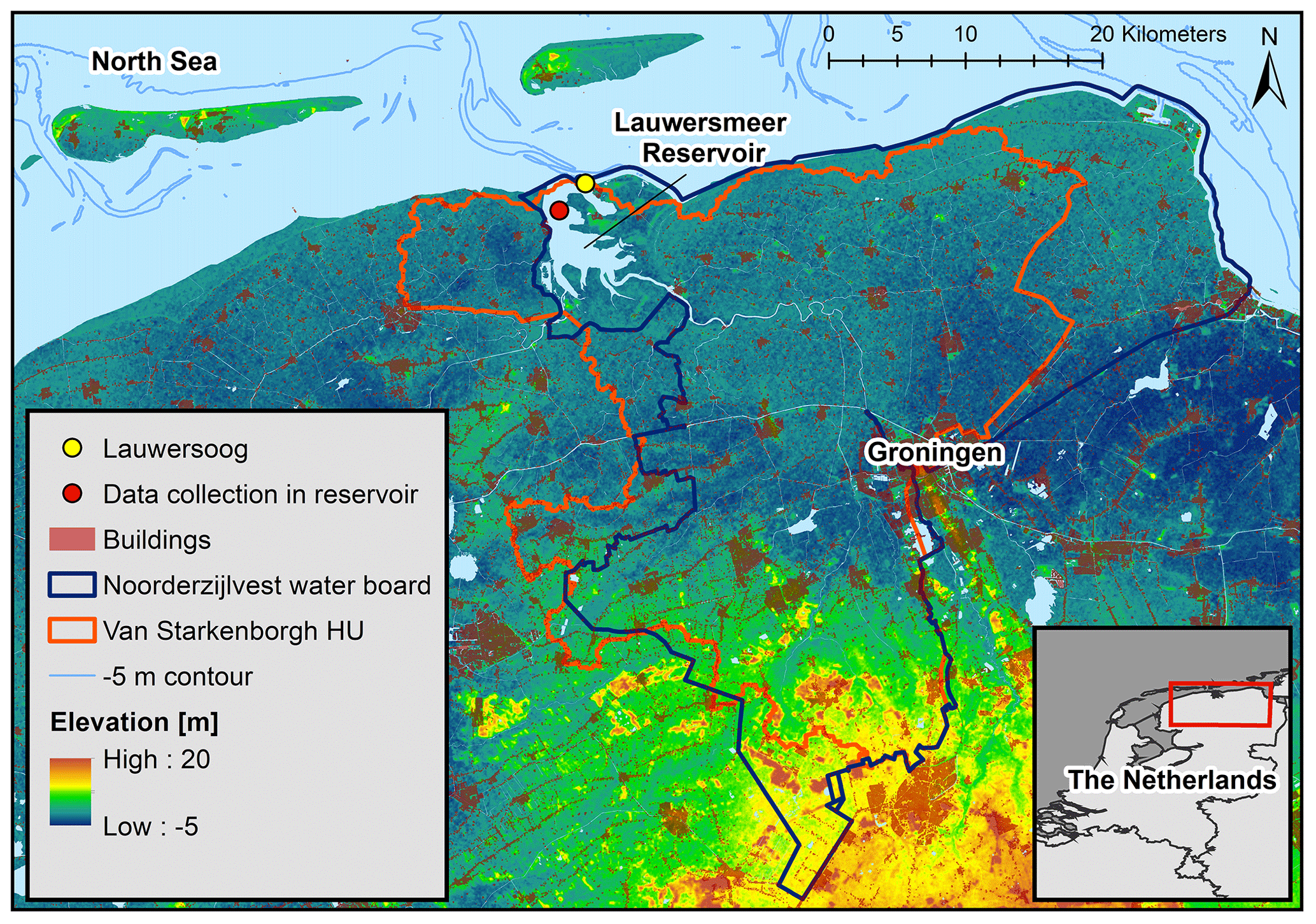
Figure 1 Overview of study site, including elevation around the area, approximate location of data collection sites, and extent of the hydrological unit (HU) and the water board that Lauwersmeer reservoir belongs to. The station Lauwersoog (yellow dot) measures the surge, and the IWL is observed inside the reservoir (red dot indicates approximate location of data collection). The bottom-right panel shows where the study site is situated in the Netherlands.

In terms of the underlying meteorological patterns, extreme winds with long fetch leading to high surges typically occur in October–December as a result of deep and extensive low-pressure systems moving from the North Atlantic region to central or northern Scandinavia (van den Hurk et al., 2015). Most extreme precipitation events occur during the summer months linked to slow-moving medium-sized low-pressure systems over northern Germany or southern Denmark (van den Hurk et al., 2015). High IWLs are caused by the interaction between these two patterns, which mostly occur in July–October. Additionally, Ridder et al. (2018) found that the majority of these types of compound events are accompanied by the presence of an atmospheric river over the Netherlands.

In this study, we build our statistical framework on the same database that was developed and applied by van den Hurk et al. (2015). The study by van den Hurk et al. (2015) empirically estimated the return periods of IWL by applying a physically based modelling chain. They used the climate simulations of the 16-member ensemble of the RCM KNMI RACMO2 (van Meijgaard et al., 2008, 2012) driven by the global climate model (GCM) EC-EARTH 2.3 (Hazeleger et al., 2012). Forced by historical emissions, the GCM was run from 1850 to 2000 with 16 different perturbations of initial atmospheric conditions. This ensemble was dynamically downscaled by the RCM at 12 km horizontal resolution for transient runs from 1951 to 2000, resulting in 800 years of historic climate. As the sixteen 50-year simulations only differ by the initial atmospheric conditions of the driving GCM, the variability of the 16 time series can be interpreted as model representations of the internal variability of the climate system (Deser et al., 2012; Hawkins and Sutton, 2009).

The bias of precipitation was adjusted for 5 d sums, and the resulting rainfall intensities were spatially averaged for the climate model grid cells enclosing the Noorderzijlvest area. After bias adjustment of wind speed and calculating a spatial average for the relevant area of the North Sea, a regression equation was applied to estimate the surge. The regression equation was calibrated to local surge conditions at the station Lauwersoog (Fig. 1). The historical astronomical tide between 1951 and 2000 using all known current tidal constituents was added to the modelled storm surge data for the complete period of 800 years. The sum of surge and tide results in a time series of still water levels (SWLs) at the North Sea. These regional simulations were then used to drive RTC-Tools, which is a hydrological management simulator (Schwanenberg et al., 2015) generating the corresponding IWL time series at hourly resolution.

To assess compounding effects, van den Hurk et al. (2015) constructed a randomized ensemble of independent drivers by shuffling the time series of model-generated precipitation and storm surge in a way that preserved climatological characteristics but removed the correlation between surge and precipitation. After adding the tidal cycle to compute the SWL, the corresponding IWLs were derived by forcing RTC-Tools with these shuffled time series of precipitation and SWL. The study by van den Hurk et al. (2015) concluded that the return period associated with the extreme 2012 IWL was almost 3 times larger for shuffled data than for the original data, which indicated the presence of compounding processes between precipitation and SWL leading to higher IWL. This is also shown by comparing the empirical joint probability density functions (PDFs) of the original and shuffled time series. However, the dependence of SWL and precipitation was weaker for the largest IWL events, which were dominated by specific neap tide conditions with a low tidal range and consequently high values of the low tides (van den Hurk et al., 2015).

3 Methods

3.1 Conceptual model

The statistical model for estimating IWL has been developed following four consecutive steps:

1. characterization of the compound event with a predictand, representing the so-called “impact” (IWL), and a set of predictors (conditioned to the impact variable), representing the underlying drivers (precipitation and SWL) of extreme IWLs;

2. development of an impact function that relates the predictand and predictors defined in step 1;

3. modelling of the joint probability distribution of the predictors, which implies finding the probability distributions to model their marginal behaviour, and identifying the best copula(s) to model their dependence structure;

4. estimating the IWL return levels by randomly generating a large number of paired precipitation and SWL synthetic events from the joint distribution obtained in step 3, which is converted to IWLs with the impact function fitted in step 2.

To reproduce the findings of van den Hurk et al. (2015), including the effect of the dependence between precipitation and SWL on return levels, this procedure is applied to both the original data set and the shuffled data (see Sect. 2). We explored statistical models of two and three dimensions (2D and 3D cases, respectively) to account for multiple predictors: a bivariate copula model accounting for the iteration of precipitation and SWL and a trivariate (vine) copula model where we separate SWL into the astronomical tide and the surge (or non-tidal residual). With this separation, we investigate whether the difference in controlling physical processes of tide and surge affects the depiction of the dependency structure causing compounding effects. The design of the analyses has followed an iterative process, with repeated feedback between the different steps. The selection of the predictors plays a crucial role in the consecutive steps and the performance of the statistical modelling framework. Specifically, the performance of the impact function is highly sensitive to the selection of the SWL (or surge in the trivariate model) predictor and has been a strong driver for the final choice of predictors. The performance of the impact function based on mean, minimum, and maximum SWL for different temporal aggregations is given in the Supplement (see Fig. S1 in the Supplement) and highlights the sensitivity to the SWL predictor.

3.2 Selection of predictands and predictors

The series of annual maxima IWLs (WL_max) is chosen as predictand to represent the impact and used to reproduce the return level plots of van den Hurk et al. (2015). In the process of predictors selection, three aspects were taken into consideration: (1) the underlying physically driving processes, including the proper representation of the compound nature of precipitation and SWL (or surge and tide in the 3D case); (2) the human management practices controlling IWL dynamics in RTC-Tools (Sect. 2); and (3) the memory of the physical system, including lags in the occurrence of drivers that might potentially affect the magnitude of the impact.

The iterative process to select the predictors is guided by the composite of all 800 WL_max and the underlying drivers (Fig. 2). Peaks in precipitation and SWL are preceding the occurrence of the annual WL_max. Opening and closing the gates of the reservoir leads to periodic fluctuations of IWL. The gates are opened during the low tide to lower IWL. If the ocean water level exceeds IWL, the gates stay closed and IWL rises due to collection of water from the surrounding watershed. For most of the 800 annual maximum events, the gates stay closed for several subsequent tidal cycles (see Fig. 2).

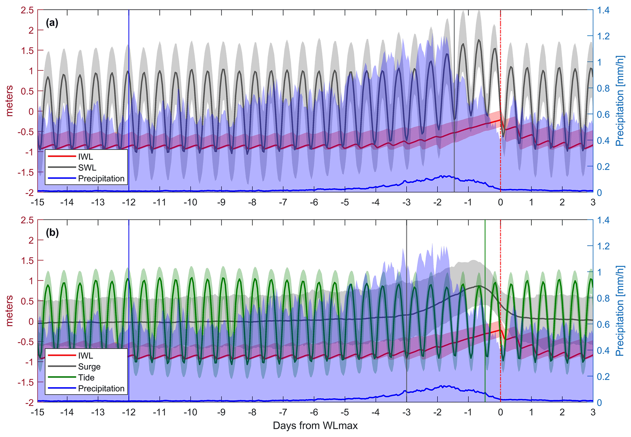
Figure 2 Composite of flooding drivers and associated IWL response for the 2D (a) and 3D (b) cases, which are computed using all 800 annual maxima events. Solid lines represent the median of all values at a given time, whereas the shaded areas depict the values between the 5th and 95th percentiles. Vertical lines indicate the time windows used for the selected predictors (see Table 1).

Table 1 Selected predictors for the 2D and 3D cases.

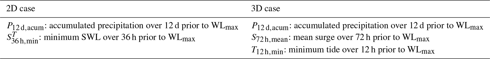
For the 2D case, we choose the following predictors: the accumulated precipitation over 12 d prior to WL_max, noted as P_12 d,acum, and the minimum SWL over the 36 h prior to WL_max, noted as $S_{\mathrm{36}\mathrm{h},\text{min}}^T$. For the 3D case, the precipitation predictor is the same as in 2D case, but the SWL is separated into tide and surge. In particular, we consider the mean surge over 72 h prior to WL_max, noted as S_72 h,mean, and the minimum tide over 12 h prior to WL_max, noted as T_12 h,min (see Table 1). The time periods of aggregation, as well as the choice of applying the arithmetic mean, minimum, or the sum, were iteratively optimized according to the performance of the impact function and its reproduction of the return period curves (see Sects. 3.3 and 3.4). We tested different temporal aggregations of the surge and tide predictors in 12 h time steps between 12 and 96 h, as this duration corresponds to the tidal cycle. The aggregation of precipitation was tested from 1 d to 20 d. All possible combinations of these predictors were used to drive the four impact function approaches (introduced in Sect. 3.3) and were evaluated by the trade-off between the performance metrics of the impact function (see Sect. 3.3) and the ability to reproduce extreme events exceeding the flood warning level (see Sect. 3.4).

The iterative process of predictor selection led to interesting insights about the physical processes behind these compound events. In terms of precipitation, Fig. 2 shows that the duration of the median peak of accumulated precipitation prior to WL_max is about 5 d, which agrees with the relevant temporal range of precipitation directly affecting IWLs identified by van den Hurk et al. (2015). Instantaneous contribution of precipitation to IWLs due to direct rainfall on the reservoir surface is small; therefore, a time lag is needed to capture the contributions from surface runoff, streamflow, and interflow caused by rainfall over the whole catchment. However, the impact function performs better for a longer aggregation time period (12 d). We argue that the precipitation prior to 5 d helps to better capture the system memory induced by soil moisture storage, as early rainfall can affect WL_max by saturating the soil. Indeed, one of the factors contributing to the largest event in 2012 was soil saturation caused by above-normal rain in the preceding weeks (van den Hurk et al., 2015). This is shown by the 95th percentile precipitation envelope in Fig. 2 that has a peak lasting more than 5 d and has a non-zero plateau for a time lag above 9–10 d.

For the 3D case, the level of the low tide during the antecedent 12 h cycle to WL_max is clearly identified as a potential predictor. It varies over time due to astronomical cycles and thus contributes to the timing of the reservoir drainage. The contribution from the surge is better captured by taking the average over the previous 72 h, which perfectly matches the duration of the surge peak observed in Fig. 2b (for both mean and extreme percentiles). It is reasonable to obtain a representative time lag of 72 h as 3 d is the mean duration of cyclones over east-central Europe (Bartoszek, 2017). When surge and tide are considered together (i.e. SWL; 2D case), a trade-off between the contribution of surge and tide is achieved by considering the minimum SWL over an intermediate time period of 36 h. Figure 2a shows that for most of the 800 events the reservoir gates were closed for at least three tidal cycles (equaling 36 h). Differing time periods (12, 24, 48, 60, and 72 h) yield a worse performance of the impact function (see Fig. S1). The minimum of the SWL is taken to account for the human management of the system. In a natural system, the SWL would directly affect the maximum IWL (e.g. Bevacqua et al., 2017), leading to the mean or the maximum SWL as likely predictors. In the study area, the human management results in the reservoir gates being opened at minimum SWL. This relationship is also reflected by the performance of the impact function for minimum, mean, and maximum SWL of 36 h as predictors (see Fig. S1).

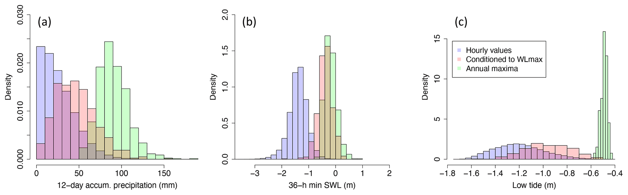
Figure 3 Density histograms for precipitation (a), SWL (b), and low tide (c) associated with all hourly time series (blue), with selected predictors (conditioned to WL_max) (pink), and with the corresponding univariate annual maxima (green).

Due to our impact-focused approach (see Sect. 3.1), the chosen predictors are conditioned to WL_max. This deviates from other studies in which an n-way sampling approach is followed (i.e. conditioning to one of the (extreme) driving variables at a time) (e.g. Ward et al., 2018). The n-way approach is usually followed when information about the impact variable is limited and/or when the focus is on identifying the driver that contributes most to compounding effects. Conditioning the drivers on the impact variable guarantees an optimal training of the impact function (Sect. 3.3), and all extreme IWLs leading to a significant impact are captured, including those that might not result from the combination of extreme univariate events. Figure 3 compares the distributions of P_12 d,acum, $S_{\mathrm{36}\mathrm{h},\text{min}}^T$, and T_12 h,min to the distribution of the corresponding univariate annual maxima. The selected predictors have notably lower values than the corresponding annual maxima, especially for precipitation and tide variables. In contrast, the conditioned SWL distribution is closer to their corresponding annual maximum distribution, which agrees with the dominant role of SWL as flooding driver leading to extreme IWLs (as seen in Sect. 3.3).

3.3 Impact function

The impact function is designed to reproduce WL_max given a set of predictors (see Sect. 3.2). We explored different approaches, including multiple linear regression (MLR), random forest (RF) (Meinshausen and Ridgeway, 2006), and artificial neural networks with stochastic gradient descent for regression (NN) (He et al., 2015; Phan, 2015). The number of trees in the RF approach was set to 50, after performing a sensitivity analysis assessing the overall performance of the approach (estimated as root-mean-square error (RMSE) via k-fold validation), depending on the number of trees. We selected 50 trees, as larger values did not lead to an increase in performance. The learning process of the NN used here is based on stochastic gradient descent, and the applied activation function is the sigmoid function. The architecture of the network is as follows: input layer with two (2D case) or three (3D case) neurons, two hidden layers with eight neurons each, and output layer with one neuron. The different regression models are evaluated by means of the RMSE, the mean absolute error (MAE), the linear (Pearson's) correlation coefficient r, and the error associated with return level estimates. This procedure was carried out for different sets of predictors in order to minimize the deviations between the WL_max simulated by the RTC-Tools and the WL_max estimated via the impact functions.

For the 2D case (Table 1), all impact function approaches simulate WL_max with an RMSE of 9 cm or less, an MAE of 7 cm or less, and r greater than 0.7 (see Fig. S2 in the Supplement). RF exhibits the best performance by means of r=0.88, MAE = 4 cm, and RMSE = 6 cm. However, none of these approaches reproduce well the extreme water levels exceeding 0 m, which have the largest impact (see Fig. S3 in the Supplement). This is due to the optimization process of the regression models, which uses a cost function penalizing the squared error of the estimated water level for each of the 800 annual maxima. The 800 annual maxima are not evenly distributed across the range of water levels between −0.5 and 0.22 m: 82 % of the samples feature water levels below −0.1 m, and 94 % of the events show water levels below 0 m. Hence, the optimized regression models are biased to reproducing WL_max between −0.5 and −0.1 m.

Table 2 Distribution of the bin-sampling classes.

Figure 4 WL_max obtained by RTC-Tools vs. WL_max obtained using MLR with the bin-sampling approach for the 2D case (see Table 1).

To overcome the underestimation of the most extreme events, we apply a bin-sampling strategy to train the impact function, optimizing the number of bins and samples per bin in an iterative manner. All 800 values are divided into 12 classes (“bins”) according to their WL_max and distributed in 5 cm steps (see Table 2). From each of these bins, 10 samples (9 for the highest bin) are randomly drawn, and the parameters of the impact function are optimized for the subset. To avoid any bias due to the randomized selection, this procedure is bootstrapped 1000 times, and the mean of the resulting parameters is taken for the final impact function. For the regression models based on machine learning (RF, NN), the implementation of this bin-sampling approach is not easy, as a simple combination of the bootstrapped parameters is not straightforward. For MLR, a combination of the linear regression factors of the 1000 random runs can well be constructed by applying the arithmetic mean. Consequently, we opt for MLR as the model of choice to define the impact function. This results in the final two-dimensional linear regression:

$$\begin{array}{ll}{\displaystyle }{\text{WL}}_{\text{max}}=& {\displaystyle }-\mathrm{0.1639}+\mathrm{0.3998}\cdot S_{\mathrm{36}\mathrm{h},\text{min}}^T\\ \text{(1)}& {\displaystyle }& {\displaystyle }+\mathrm{0.0027}\cdot P_{\mathrm{12}\mathrm{d},\text{acum}}.\end{array}$$

The comparison of WL_max simulated by the RTC-Tools and WL_max estimated via Eq. (1) is shown in Fig. 4. After standardization of the predictors by $\stackrel{\mathrm{̃}}{X}=(X-\stackrel{\mathrm{‾}}{X})/X^{\text{sd}}$, where $\stackrel{\mathrm{‾}}{X}$ and X^sd are the corresponding mean and standard deviation, the dominant role of SWL compared to precipitation is evident:

$$\begin{array}{ll}{\displaystyle }{\text{WL}}_{\text{max}}=& {\displaystyle }-\mathrm{0.1932}+\mathrm{0.1033}\cdot {\stackrel{\mathrm{̃}}{S}}_{\mathrm{36}\mathrm{h},\text{min}}^T\\ \text{(2)}& {\displaystyle }& {\displaystyle }+\mathrm{0.0639}\cdot {\stackrel{\mathrm{̃}}{P}}_{\mathrm{12}\mathrm{d},\text{acum}}.\end{array}$$

For the 3D case (Table 1), we obtained:

$$\begin{array}{ll}{\displaystyle }{\text{WL}}_{\text{max}}=& {\displaystyle }-\mathrm{0.2645}+\mathrm{0.4652}\cdot S_{\mathrm{72}\mathrm{h},\text{mean}}+\mathrm{0.3434}\cdot T_{\mathrm{12}\mathrm{h},\text{min}}\\ \text{(3)}& {\displaystyle }& {\displaystyle }+\mathrm{0.0028}\cdot P_{\mathrm{12}\mathrm{d},\text{acum}}.\end{array}$$

which has the following standardized version:

$$\begin{array}{ll}{\displaystyle }{\text{WL}}_{\text{max}}=& {\displaystyle }-\mathrm{0.1972}+\mathrm{0.1110}\cdot {\stackrel{\mathrm{̃}}{S}}_{\mathrm{72}\mathrm{h},\text{mean}}+\mathrm{0.0644}\cdot {\stackrel{\mathrm{̃}}{T}}_{\mathrm{12}\mathrm{h},\text{min}}\\ \text{(4)}& {\displaystyle }& {\displaystyle }+\mathrm{0.0663}\cdot {\stackrel{\mathrm{̃}}{P}}_{\mathrm{12}\mathrm{d},\text{acum}}.\end{array}$$

The 3D impact function shows slightly better performance metrics than in the 2D case (r: 0.76, RMSE: 0.085 m, MAE: 0.066 m vs. r: 0.71, RMSE: 0.091 m, MAE: 0.071 m; see Fig. S4 in the Supplement). However, the 2D model better reproduces the extreme events over the flood warning level, which is 7 cm Normaal Amsterdams Peil (NAP). For these events, the RMSE of the 2D model amounts to 0.034 m, whereas the RMSE of the 3D model amounts to 0.078 m. This agrees with the performance of the return level estimations: the 3D model performs slightly worse (generally more tendency to underestimate than the 2D model; see Figs. S3 vs. S5).

3.4 Joint probability density function and return levels

The joint distribution of the selected predictors is modelled via a copula function (Sklar, 1959; Nelsen, 2007) (see Sect. 1 in the Supplement). The selection of the marginal distributions and the dependence structure of the predictors is crucial for a robust assessment of WL_max. The overall methodology to obtain the return level estimates is similar between the 2D and 3D cases (see Sect. 3.1) and implemented as follows. (1) To separate marginal and dependence modelling, data are ranked and transformed to be uniform in the unit (hyper)square using rank statistics; (2) copula family and parameters are fitted to these uniform data with the maximum pseudo-likelihood estimator (Kojadinovic and Yan, 2010); (3) a total of 40 copula types are considered (VineCopula R package, version 2.3.0), selecting the one leading to the lowest Akaike information criterion (AIC) (Schepsmeier et al., 2015). The adequacy of the selected copula model is assessed using a goodness-of-fit test based on Kendall's processes (Genest et al., 2009; Wang and Wells, 2000); (4) suitable marginal distributions for the (unranked) defined predictors are identified, testing a wide range of distributions commonly used in hydrologic analysis and selecting the one with the best fit (lowest AIC; Sakamoto et al., 1986); (5) the joint probability distribution of the considered predictors is obtained with the best fitted copula(s) and marginals; (6) assuming that the selected copula accurately represents the tails of the distribution (an inherent assumption of the majority of studies of this type), simulated events from this joint distribution are obtained by sampling uniform data from the copulas; (7) sampled events are converted to real units with the previously fitted marginals; and finally (8) the obtained synthetic samples are used to estimate WL_max via the impact function explained in Sect. 3.3. Note that the fitted marginals are intentionally not used for the copula fitting in order to make the choice of the copula(s) totally independent from the choice of the marginal(s) (Genest and Favre, 2007).

Once water levels have been calculated, the associated return periods are obtained using Weibull plotting positions (Makkonen, 2006). Compounding effects are assessed by comparing the return levels obtained by fitting the copula model and the marginals to the dependent and the shuffled (independent) data (Sect. 2). Copula models are used to generate many synthetic events of paired precipitation and surge (up to 100 000) to produce stable return level estimates of WL_max up to a 10 000-year return period. Although producing a 10 000-year data set from 800 years of empirical data entails dealing with large uncertainties, especially for the highest return levels, we chose that number because it establishes the standard level of protection in many places in the Netherlands, especially those exposed to severe flooding (Bouwer and Vellinga, 2007).

4 Results and discussion

The results of the statistical modelling framework are presented here. We find that the model with three predictors (3D case), i.e. precipitation, surge, and tide, does not generally outperform the model with two predictors (2D case), i.e. precipitation and SWL (see Table 1). Even though the impact function of the 3D model shows slightly better performance metrics than the impact function of the 2D model, the 2D model shows a closer reproduction of the extreme events over the flood warning level (see Sect. 3.3). Based on this evaluation and following the parsimony principle, results of the 2D case are presented in the article, leaving most of results of the 3D case in the Supplement.

4.1 Dependence structure between SWLs and precipitation

In order to better understand the underlying factors leading to WL_max, this section explores the dependence structure between SWL and precipitation (2D case) using Kendall's rank correlation coefficient (τ) (Kendall, 1938) and the joint PDF (probability density function) of $S_{\mathrm{36}\mathrm{h},\text{min}}^T$ and P_12 d,acum. Different sources of variability are assessed, with a special focus on the internal variability of the climate system.

4.1.1 Interpretation of τ: dependence vs. independence

The τ estimate between the defined predictors, i.e. $S_{\mathrm{36}\mathrm{h},\text{min}}^T$ and P_12 d,acum, for the dependent data set amounts to −0.05, differing from zero correlation at the 95 % significance level. To further investigate the compound nature of the two predictors, the same correlation is calculated using the shuffled (independent) data. In this case, τ amounts to −0.15. The negative τ between $S_{\mathrm{36}\mathrm{h},\text{min}}^T$ and P_12 d,acum is arguably related to the positive contribution of both the SWL and precipitation to IWL and therefore the negative slope of the WL_max isolines as a function of these predictors: lower values of one driver can be compensated by higher values of the other driver to generate a given water level. This is illustrated with a simple theoretical example in Sect. 2 in the Supplement (and Fig. S6 in the Supplement). This example highlights that when drivers positively contribute to increasing the impact, then impact-focused predictors (i.e. predictors conditioned to the impact) can have a negative τ for positively correlated drivers. This example also illustrates that comparing the τ between conditioned predictors with that obtained from an independent data set provides information about the dependence pattern among drivers. In our study, the τ obtained from the predictors of the dependent case exceeds that obtained from the independent case by +0.10, which arguably indicates a positive dependence pattern between SWL and precipitation. Similarly, the corresponding joint PDFs (see Sect. 3.4) show the increased probability of having both extreme $S_{\mathrm{36}\mathrm{h},\text{min}}^T$ and P_12 d,acum (leading to extreme IWLs) as obtained from the original data, in comparison to the independent case (see shaded orange area in Fig. 5). This agrees with the findings of van den Hurk et al. (2015) obtained empirically.

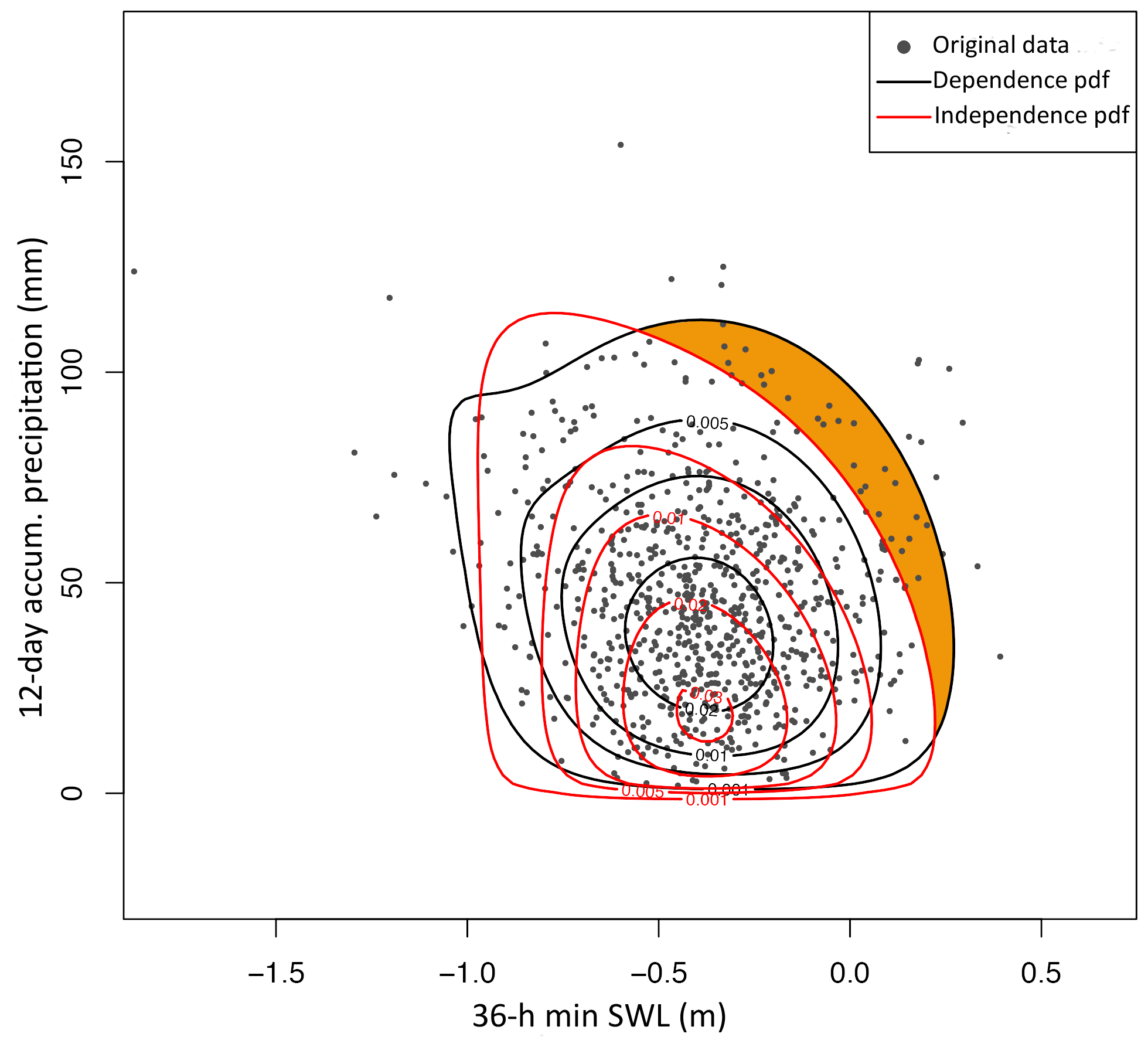
Figure 5 Scatter plot of $S_{\mathrm{36}\mathrm{h},\text{min}}^T$ and P_12 d,acum and its joint PDF corresponding to original data (black) and shuffled data (red). Shaded orange area highlights the increased probability of extreme $S_{\mathrm{36}\mathrm{h},\text{min}}^T$ and P_12 d,acum for the original data.

In summary, as a result of our impact-focused approach, the correlation between the defined predictors (the explanatory variables of the impact function) does not duplicate the dependence between drivers (precipitation and SWLs) leading to extreme IWLs. Such conditioning complicates the interpretation of the dependence structure and compound effects but optimizes the performance of the impact function and hence the performance of the statistical modelling of return level estimates. It is therefore important to distinguish between the correlation/dependence between the selected predictors and the correlation/dependence between the drivers (although the former informs the latter). There is certainly a number of ways one could define the drivers to better portray such dependence, but regardless of that, when broadly speaking about positive dependence/correlation between drivers, one would refer to the increased likelihood of concurrent drivers that contribute to impactful events, i.e. the so-called “compound effects”. As illustrated by the example in the Supplement and shown in Fig. S6, positive compound effects are not necessarily associated with positive values of τ between the corresponding conditioned predictors. Compound effects can still be investigated by comparison with estimates obtained from shuffled (independent) data, expressed by either τ or the associated return level estimates (as shown in Sect. 4.2). For example, the positive dependence between surge and precipitation is not depicted by the plain correlation between $S_{\mathrm{36}\mathrm{h},\text{min}}^T$ and P_12 d,acum but by the positive shift between the corresponding correlations obtained for the original and shuffled data. Moreover, although such dependence has an impact on IWL return levels (Sect. 4.2), the fact that τ between $S_{\mathrm{36}\mathrm{h},\text{min}}^T$ and P_12 d,acum is weak also indicates that the dependence between drivers is not very strong.

4.1.2 Seasonal variability

To increase process understanding and strengthen the link between the statistical framework and the physical processes, we investigate the seasonal variability of the dependence structure between $S_{\mathrm{36}\mathrm{h},\text{min}}^T$ and P_12 d,acum; τ is lowest during winter (DJF: −0.13), increases in spring (MAM: 0.01) and summer (JJA: 0.10), and drops again in the fall (SON: 0). This variability is caused by the underlying physical factors leading to extreme IWLs, which depend on the seasonality of surge and precipitation in this area, as explained in Sect. 2 (see also Fig. S7 in the Supplement). In general, SWL contributes more to WL_max than precipitation, which is explained by the dominant role of surge (see Sect. 3.3). The monthly frequency of the annual maximum of the minimum SWL over 36 h time windows (without being conditioned to WL_max) shows the highest values between September and December (see Fig. S7b), which is similar to the seasonal course of the monthly frequency of WL_max events (see Fig. 6). In winter, the contribution of SWLs intensifies, and it becomes the most predominant driver. This agrees with the lowest seasonal correlation between $S_{\mathrm{36}\mathrm{h},\text{min}}^T$ and P_12 d,acum obtained for this season. In summer, the likelihood of heavy precipitation increases (see Fig. S7b), which increases the chance of compound surge and precipitation leading to extreme IWLs, which is reflected in a larger correlation between $S_{\mathrm{36}\mathrm{h},\text{min}}^T$ and P_12 d,acum in this season.

Figure 6 Frequency of WL_max events occurring each month (a), monthly mean of WL_max (b), $S_{\mathrm{36}\mathrm{h},\text{min}}^T$ (c), and P_12 d,acum (d).

We also investigated separating the WL_max events into seasonal clusters to build the impact function. It did not lead to an improved model representation of WL_max events in terms of RMSE (not shown) but led to increased uncertainty for large return periods due to a smaller statistical sample. The latter was particularly critical for spring and summer, as the number of annual maxima events is unevenly spread over the annual cycle, and few of these events occur in the warmer seasons. The majority of WL_max occurs in the fall (Fig. 6a) for which IWL is also larger (Fig. 6). Therefore, we continue our analysis with all-year results and ignore the seasonal signature of IWL return levels.

4.1.3 Variability as a function of tides

The correlation between SWLs and precipitation varies as a function of the tide elevation, as shown in Table 3. There is a tendency of intensified positive dependence between $S_{\mathrm{36}\mathrm{h},\text{min}}^T$ and P_12 d,acum for higher T_12 h,min, i.e. for smaller tidal ranges and higher low tides. This is apparent for both the surge predictor in the 3D case (S_72 h,mean) and the SWL predictor ($S_{\mathrm{36}\mathrm{h},\text{min}}^T$) in the 2D case. This result is in contrast with findings of van den Hurk et al. (2015), who argued that surge and precipitation had a weaker correlation for most extreme WL_max which they attributed to low tidal range between high and low tides, as extreme IWLs tend to occur in neap tide conditions.

Table 3 τ estimate between $S_{\mathrm{36}\mathrm{h},\text{min}}^T$ and P_12 d,acum, as well as S_72 h,mean and P_12 d,acum, as a function of T_12 h,min.

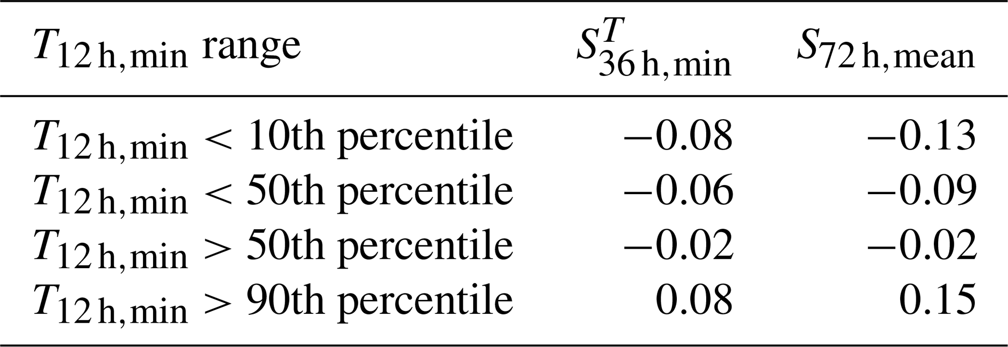
Indeed, there is a positive dependence between T_12 h,min and WL_max (τ=0.10), which is reflected by a positive shift of the low tides prior to WL_max with respect to the distribution of all low tides (see Fig. 3c). Also, the upper 10th percentile of T_12 h,min occurs in the fall season (Fig. S8 in the Supplement), when the largest water level events tend to occur (Fig. 6). This is consistent with the lower amplitude in the major tidal constituents in September/October in the North Sea (Gräwe et al., 2014). However, P_12 d,acum and particularly $S_{\mathrm{36}\mathrm{h},\text{min}}^T$ have a greater impact on WL_max than T_12 h,min. This is reflected in their respective rank correlation coefficients: τ=0.23 (P_12 d,acum and WL_max) and τ=0.42 ($S_{\mathrm{36}\mathrm{h},\text{min}}^T$ and WL_max) (τ=0.36 for S_72 h,mean and WL_max).

Moreover, we argue that it is not evident whether the correlation between surge and precipitation is weaker for extreme IWL return levels. The tail of the return level plot is affected by sampling variability. As an example, we calculated the variation of the range of uncertainty in estimating the 800-year return level by sampling 800 and 100 000 events, respectively, from our statistical framework for both the independent and dependent cases. We empirically obtain that, with a single 800-year realization, there is a probability of 12 % of the 800-year return level from original data to be smaller than the 800-year return level based on the shuffled data. However, when sampling 100 000 events, the probability is virtually zero. A visualization of this example is given in Fig. S9 in the Supplement. This indicates that estimates about the variability of the role of driver dependence on generating high IWLs might be subject to sampling uncertainty for return periods of similar value as the length of sample size. In any case, clustering by tides reveals that a weaker correlation between $S_{\mathrm{36}\mathrm{h},\text{min}}^T$ and P_12 d,acum is more likely to happen with lower T_12 h,min and therefore larger tidal ranges. Separating the statistical analysis into tidal clusters did not lead to improvement in terms of RMSE (not shown), but we further investigate the tide effect in the 3D case (see Sect. 4.2).

4.1.4 Climate variability

The internal climate variability can have profound effects on the evaluation of compound flooding hazards, as the dependence structure and correlation of predictors is highly modulated by how climatic variables affect those predictors. To assess the effect of the internal variability of the climate system on the estimation of the correlation between the selected predictors, the correlation between $S_{\mathrm{36}\mathrm{h},\text{min}}^T$ and P_12 d,acum is estimated for each individual member of the SMILE (50 years per member) (Fig. 7a). The correlation ranges between −0.18 and 0.04, and its mean is −0.05 (equal to the value obtained using 800 years of data). However, none of these values are statistically significantly different from zero, given that reducing the sample size increases the chance of obtaining non-statistically significant correlation estimates at a given significance level (here 95 %).

Figure 7 Variability of copula fitting among the sixteen 50-year runs for original (a) and shuffled data (b–k). Red dots indicate the independence test is rejected.

The correlation difference between original and shuffled data (which indicates the positive dependence between surge and precipitation; see Sect. 4.1.1) is largely affected by climate variability. Figure 7b–k shows the variability of τ and its statistical significance (at the 95 % confidence level) for the shuffled data, which leads to a range of the correlation difference from −0.26 to 0.36 accounting for all 10 shuffles. This indicates that internal climate variability has a pronounced impact on the estimation of compound effects. Section 4.2 further investigates this matter in terms of the return levels estimates.

4.2 Return water level estimates: compound effects and climate variability

In this subsection, the proposed statistical framework is evaluated in terms of the IWL return levels, using the empirical estimates provided by van den Hurk et al. (2015). We also describe the results from the marginal and dependence analysis, as well as the sensitivity of the three methodological components (impact function, marginal distributions, and dependence assessment) to internal climate variability represented by the inter-run variability across the 16 SMILE members.

4.2.1 Joint probability density function

To estimate WL_max based on the 2D model, the normal and the Weibull distributions are selected as the best-fit probability distributions to fit the marginals for SWL and precipitation, respectively. To represent the joint behaviour of the two selected predictors, the rotated Tawn type-I copula is selected with associated negative τ (−0.05). As explained in Sect. 4.1.1, a negative τ for the predictors is compatible with positive dependence between drivers due to the impact-focused approach. The Tawn copula is an asymmetric extension of the Gumbel copula. This asymmetry feature agrees with the scatter plot in Fig. 5. When $S_{\mathrm{36}\mathrm{h},\text{min}}^T$ is low, WL_max events occur for relatively high P_12 d,acum (compared to the other WL_max events), while $S_{\mathrm{36}\mathrm{h},\text{min}}^T$ does not need to be particularly high when P_12 d,acum is low. This is due to the asymmetric contribution of P_12 d,acum and $S_{\mathrm{36}\mathrm{h},\text{min}}^T$ to WL_max with the surge predictor being the dominant predictor, as seen in Sect. 3.3.

Similarly, in the 3D case a normal distribution fits both tide and surge accurately, and precipitation is well described by a Weibull distribution. The vine structure that most accurately describes the dependence between these three variables contains the following bivariate copulas: rotated BB1 (270^∘) (dependence between P_12 d,acum and T_12 h,min), Frank (dependence between T_12 h,min and $S_{\mathrm{72}\mathrm{h},\text{mean}}^T$), and rotated Clayton (90^∘) (dependence between T_12 h,min given $S_{\mathrm{72}\mathrm{h},\text{mean}}^T$, and P_12 d,acum given T_12 h,min). A visual representation of the structure of the regular vine is given in Fig. S10 in the Supplement.

4.2.2 Compound effects

Generally, the calculation of return periods for independent drivers might be performed by forcing an independence copula or by randomly sampling from the fitted marginals directly (Genest and Favre, 2007). However, we selected the predictors conditioned to WL_max in order to ensure a close reproduction of WL_max calculated by the impact function. This step affects the correlation between the predictors (see Sect. 4.1.1 and Fig. S6), which is why zero correlation between SWL and precipitation does not equal to zero correlation between $S_{\mathrm{36}\mathrm{h},\text{min}}^T$ and P_12 d,acum. In fact, τ associated with $S_{\mathrm{36}\mathrm{h},\text{min}}^T$ and P_12 d,acum obtained from the shuffled data (independent case) amounts to −0.15. Hence, our statistical framework cannot reproduce the return period curves of the shuffled data when using an independent copula to describe the dependence structure between $S_{\mathrm{36}\mathrm{h},\text{min}}^T$ and P_12 d,acum. Therefore, to quantify the compound nature of WL_max, we used the return levels estimated from the independent drivers (shuffled data) as reference.

To assess the independent case, we use the predictors defined in Table 1 and obtained from the shuffled data (see Sect. 2) and we follow the same procedure as for the dependence case to obtain the corresponding IWL return levels. Results for both cases are shown in Fig. 8 (2D case) and Fig. S11 in the Supplement (3D case), where IWL return level estimates are compared against the empirical estimates by van den Hurk et al. (2015). Both 2D (Fig. 8) and 3D (Fig. S11) approaches reproduce compounding effects with high skill, as shown by a comparison between the empirical and simulated data for equivalent return periods via RMSE. The RMSEs of the 2D case (dependence and shuffles) amount to 0.02 m, where the RMSEs of the 3D case (dependence and shuffles) amount to 0.019 m. The small difference of 1 cm between the performance of the 2D and 3D cases shows that adding complexity to our framework can only slightly improve the performance. The almost equivalent performance of both models led us to present the simpler model in the article as a preferable choice, and we leave the more complex model in the Supplement. In addition, as seen later on in Sect. 4.2.3, the 3D model is more sensitive to climate variability uncertainty.

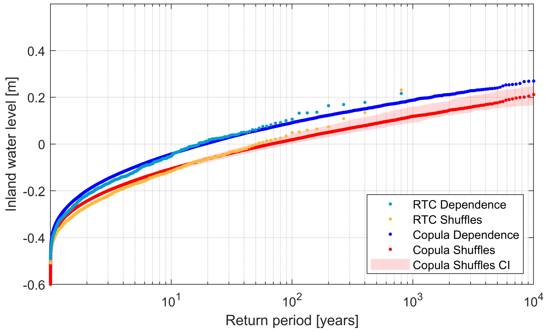
Figure 8 IWL return level against estimated return period using a bivariate copula model (2D case). Blue and red dotted lines depict the dependence and independence cases, respectively. Transparent red denotes confidence intervals, which account for the uncertainty range between the 5th and 95th percentiles, as computed from all shuffles. Light blue dots and orange dots represent the return values empirically obtained by van den Hurk et al. (2015).

Despite overall good performance, both 2D and 3D approaches differ slightly from the empirical data for the highest return periods. However, as noted in Sect. 4.1.3., the tail of the return plot is sensitive to the number of simulations used to obtain such estimates (see Fig. S9). This explains the disagreement between the modelled and the empirical estimates for large return periods (modelled lines are more parallel than empirically estimated lines), as we obtained these curves by simulating larger samples (100 000 events) than the empirical analysis (800 events).

4.2.3 Climate variability

In Sect. 4.1.4 we showed the effect of the climate variability on the predictors' dependence structure by exploring τ. Here, we explore the effect of climate variability on each component of our statistical framework: the impact function, the marginal distribution, and the copula function. In particular, we investigate the impact on (1) the estimates of IWL return levels corresponding to the dependence case (Fig. 9) and (2) the ratio of the estimated return periods from the shuffled predictors (RP_s) to those derived by accounting for dependence between predictors (RP_d) (Fig. 10). This ratio indicates the bias in return period calculation if dependence between drivers was ignored and is used as a proxy of the compound effects, i.e. the increased probability of extreme IWL due to the positive dependence between SWLs and precipitation. Table 4 specifies the settings used to produce Figs. 9 and 10.

Figure 9 IWL return level against estimated return period using a bivariate copula. Blue dots depict the return level estimates obtained using the proposed statistical framework (using 800 years of data). Transparent green illustrates the uncertainty associated with internal climate variability, represented by bounds computed using the 5th and 95th percentiles from all 50-year ensembles. Opaque green shows the median value computed from all ensembles. This is assessed for each component of the methodology: (a) 50-year ensembles are used for all components; (b) same as (a) but MLR impact function is trained with standard sampling using 800 years of data; (c) same as (b) but using bin-sampling approach; (d) 50-year runs are used for copula fitting only; (e) 50-year runs are used for SWL marginal fitting only; and (f) 50-year runs are used for precipitation marginal fitting only (see Table 4).

Figure 10 Compound effect (estimated as ratio between return periods as obtained from shuffled and original data) against IWL return level using a bivariate copula. Blue dots depict the values obtained using the proposed statistical framework (using 800 years of data). Transparent green illustrates the uncertainty associated with internal climate variability, represented by bounds computed using the 5th and 95th percentiles from all 50-year ensembles. Opaque green shows the median value computed from all ensembles. This is assessed for each component of the methodology: (a) 50-year ensembles are used for all components; (b) same as (a) but MLR impact function is trained with standard sampling using 800 years of data; (c) same as (b) but using bin-sampling approach; (d) 50-year runs are used for copula fitting only; (e) 50-year runs are used for SWL marginal fitting only; and (f) 50-year runs are used for precipitation marginal fitting only (see Table 4).

Table 4 Settings used in subpanels of Figs. 9 and 10 to assess climate variability (green).

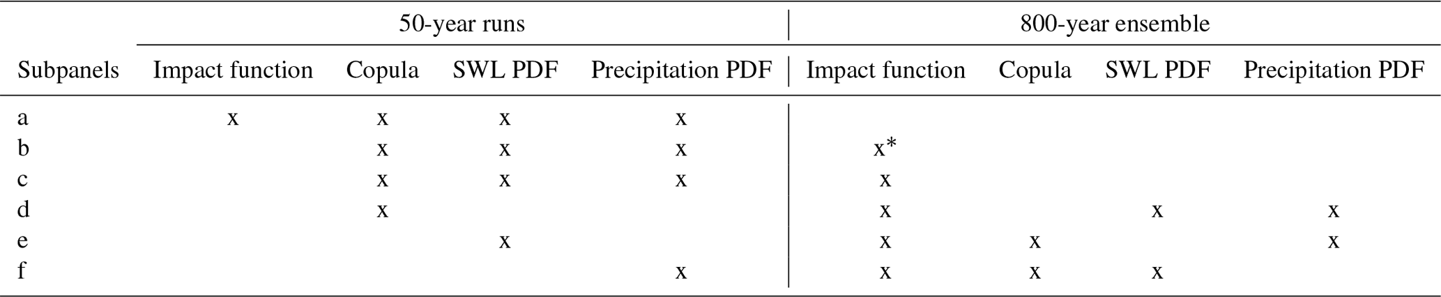
^* Impact function based on MLR with standard sampling; i.e. the bin-sampling approach is not implemented.

First, Fig. 9a shows IWL return level estimates for the bivariate case, and associated variability computed from all subsets of 50 years for each component. Large uncertainty intervals surround the average of values based on these 50-year subsets, and this average return period curve is shifted downwards compared to the 800-year reference curve approach. The general tendency of the regression model to simulate lower return levels, especially for high return periods, is mainly caused by the fact that we cannot perform the bin-sampling approach with only 50 years of data. Indeed, not performing the bin-sampling procedure when using the entire data set (800 years of data) leads to a very similar result (Fig. 9b). The training of the impact function by means of bin-sampling eliminates the tendency to simulate lower return levels, as shown in Fig. 9c where the proposed function (Eq. 1) is applied while using 50-year ensembles for marginal and copula fitting. Yet, uncertainty is not reduced when using the bin-sampling approach with 800 years, which illustrates that most uncertainty related to internal climate variability is introduced by other framework components. Similar to Fig. 9a and c, Fig. 10a and c show the variability of the return period ratio when 50-year ensembles are used for all framework components and when the impact function with bin sampling is applied, respectively. Return period ratios are likely to vary significantly when only 50 years of data are available as noted by the large green intervals (Fig. 10a and c). Furthermore, there is a tendency to underestimate compounding effects even when the impact function with bin sampling is used (Fig. 10c).

Second, the effect of climate variability on copula fitting and its impact on the estimation of IWL return levels are shown in Fig. 9d. Here, we apply the optimally trained impact function and use the entire data set to fit the marginals while using 50 years of data for the copula fitting. As expected, the copula fitting does not generate significant differences between the 50-year runs as τ becomes virtually zero for all 50-year runs (see Sect. 4.1.4, Fig. 7a). This low variability induced by copula fitting, however, does not imply that bivariate copula models are generally unaffected by climate variability. In this study, copulas do not play a significant role in the estimation of IWL return periods for the 2D dependence case. While there is dependence among drivers, Kendall's τ for the 800 years of the selected (conditioned) predictors is very close to zero. Hence, shortening the data set length does not affect the reliable estimation of IWL in terms of copula modelling for the dependence 2D case. Nonetheless, climate variability does affect the estimation of IWL for the shuffled data (not shown) due to the inherent variability in the corresponding τ and copula fitting (Fig. 7b–k). This suggests that the use of short records probably affects the estimation of compound effects. Indeed, Fig. 10d clearly illustrates that the use of small samples to fit the copulas tends to lead to an underestimation of compound effects. Climate variability also causes a large uncertainty of return period ratios when copulas are derived from 50-year time series.

Third, to explore the effect of climate variability on marginal fitting, we tested and fitted different suitable probability distributions to the marginals of all 50-year ensembles, while using 800 years for copula fitting and the optimally trained impact function to transform simulations. A comparison between Figs. 9e, 10e, 9f, and 10f shows the uncertainty associated with SWL and precipitation data marginal fitting. We find that most uncertainty in estimating IWL return levels is associated with the fitting of the SWL distribution (Fig. S12a in the Supplement). This uncertainty is reflected in the IWL estimates, since the SWL is the predominant driver. Furthermore, comparing Fig. 10d–f reveals that the tendency to underestimate compounding effects in Fig. 10d is mainly introduced by the copula fitting. Hence, short records might hinder a proper estimation of compound effects due to poor copula fitting.

An analogous uncertainty analysis was performed for the trivariate case (Fig. S13 in the Supplement), examining the uncertainty associated with each component of the proposed statistical framework. Although generally similar insights were obtained as for the bivariate uncertainty assessment, some differences are worth mentioning. For instance, copula fitting (Fig. S13c) presents larger uncertainty intervals than for the bivariate case. As the predictors are defined differently in the trivariate case, the correlation between them has also changed and has become crucial to reproduce IWL dependence curves. In addition, separating SWL into surge and tidal range reveals that marginal fitting uncertainty is mostly caused by surge, followed by tides (see Fig. S12c and d). Although tidal range is an important factor determining the occurrence of extreme IWL in our study case, the surge is the most important variable explaining the behaviour of IWL (as seen in Sect. 3.3, Eq. 4).

In summary, we find that the internal variability of the climate system represented by the variability between the sixteen 50-year members induces a large uncertainty range at every step of our statistical framework. The impact function cannot be properly calibrated with 50-year data. Furthermore, compound effects tend to be underestimated when applying short records to fit the copula.

5 Conclusions

In this study we developed an impact-focused copula-based multivariate statistical framework that produces robust estimates of compound extreme inland water return levels (IWL) for a highly managed reservoir in the Netherlands. This work was motivated by a near-flooding event in 2012, which was empirically analysed by van den Hurk et al. (2015) based on a single model initial-condition large ensemble (SMILE) consisting of a set of sixteen 50-year simulations. Like in van den Hurk et al. (2015), we used these 16 members as 800 years of current climate conditions that account for the internal variability of the climate system. In particular, we defined simulations of the IWL as the impact variable and still water level (SWL) and precipitation as the underlying drivers. To assess compounding effects, we used a randomized ensemble of independent drivers which van den Hurk et al. (2015) obtained by shuffling the 50-year runs, thereby removing the correlation between surge and precipitation but preserving their climatological characteristics.

The high degree of human management in the system studied poses a challenge to select suitable predictors and subsequently developing an impact function that is skilful at predicting IWLs as a function of such predictors. We considered bivariate and trivariate models (which were implemented after separating SWL into surge and tidal ranges), resulting in similar performance at reproducing the return levels by van den Hurk et al. (2015). Predictors were selected after an iterative process (guided by composite analysis) to optimize the performance of the impact function and return level estimates. After testing several options, we defined WL_max (annual maxima of IWL) as predictand, and the 12 d cumulative precipitation and 36 h minimum SWL prior to WL_max as predictors. The resulting impact function is a multilinear regression model with a bin-sampling approach that gives more weight to the most extreme IWL events in the calibration process. SWL, and in particular surge, is found to be the predominant driver.

Our statistical model shows that, although not very strong, the dependence structure between drivers (SWL and precipitation) contributes to increased IWL return levels, as was found empirically by van den Hurk et al. (2015). Due to the conditioning of the proposed predictors on the impact variable, the positive dependence is implicitly assessed by comparing the joint probability distributions and return level estimates to results obtained from the shuffled (independent) data. Some extreme IWLs are primarily driven by surge (especially those occurring in winter), but compound processes increase for other seasons. A copula-based multivariate statistical framework is generally able to capture the complex compound nature of precipitation and SWL and to reproduce extreme IWL return levels at the local scale, also under conditions where the strong management of the hydrological system was not explicitly represented in the underlying data.

Furthermore, we performed a unique uncertainty assessment to explore the impact of internal climate variability on the return water level estimates. The use of a subset of 50 years of data (which is the typical maximum record length available from observational records) was tested for different components of our framework, namely the impact function, the copula fitting, and the marginal fitting. Using an impact function with standard sampling leads to a consistent underestimation of the return levels, as the bin-sampling approach is not feasible for 50 years of data. The marginal fitting of surge is the factor that most contributes to uncertainty of the return level estimates. For the 2D case, copula fitting with small samples does not lead to additional uncertainty in the return level estimates. However, low variability provided by copula models is due to their insignificant role in the estimation of IWL return level for the dependence 2D case, as correlation between the selected predictors (conditioned to IWL annual maxima) is close to zero. Indeed, the 2D case could be simplified with an independent copula with no major impact on return level estimates. Yet, dependence models are still crucial to reproduce and understand compounding effects, as the dependence structure does play a significant role when modelling the shuffled data. The use of 50-year subsets leads to a tendency to underestimate the increased probability of extreme IWL due to inherent positive dependence between SWL and precipitation. For the 3D case, increased dependence between the predictors and a larger model complexity leads to increased uncertainty induced by copula fitting when shorter records are used. We emphasize that these findings are highly case specific and dependent on the chosen statistical framework. However, this case study illustrates that internal variability can be a major source of uncertainty for estimation of extreme IWLs and the associated compound effects.

Although the results presented here are site specific, the general framework can be transferred to other locations, given the availability of relatively long overlapping records of flooding drivers and impact variables. If the size of the database needs to be extended prior to developing a multivariate statistical framework, a regional climate model (RCM) SMILE and a hydrological management simulator to derive empirical estimates could be used (e.g. van den Hurk et al., 2015). Depending on the size of the ensemble and spatial resolution of the RCM, large computational resources may be required. Defining appropriate predictors leading to a satisfying performance of the impact function depends on the hydrological characteristics and management of a given system. For systems with low or no management, we would expect a more straightforward construction of an impact function, but appropriate lags between drivers and impacts should be accounted for. Characterizing probability distributions that precisely describe the marginals and fitting copulas that accurately capture the dependence structure largely depend on data availability.

The proposed framework assumes that waves are not an important driver of extreme IWLs, and only low-frequency sea-level components are accounted for. This is reasonable considering the characteristics of the study area: (1) sheltering effects of barrier islands protecting from extreme wave climate and (2) shallow waters inducing wave breaking for large wave heights. In contrast, surge is a relevant driver of extreme SWLs in such shallow water environments. However, if our framework were to be implemented in areas exposed to extreme waves, ocean wave predictors would need to be included in the model. Yet the proposed framework described in Sect. 3 would still be valid.

The surge is calculated from the meteorological forcing for all relevant timescales, from daily to multi-annual, using the empirical relationship between surge and model-generated wind. Apart from the astronomical tide, no other sources of variability are incorporated into the sea-level records. Therefore, the main limitation of this study is the exclusion of long-term nonstationary sea-level processes, such as sea-level rise which plays a large role in increasing extreme SWLs (Taherkhani et al., 2020). However, since our focus is on the assessment of historical extreme sea-level climate with the focus on the effect of climate variability, this assumption is reasonable.

We conclude that larger sample sizes than what we would typically obtain from observational data are needed in order to reproduce representative extreme IWL statistics. Furthermore, observations are one possible realization of the climate system within its boundaries of internal variability. Therefore, short records present challenges to properly estimate the relationship between predictors and predictand, marginal distributions, and dependence patterns. Large sample sizes made available from the application of SMILEs are valuable to investigate compound events and quantify the associated uncertainties induced by internal variability.