the Creative Commons Attribution 4.0 License.
the Creative Commons Attribution 4.0 License.
 | 17 Jun 2021
Low and contrasting impacts of vegetation CO2 fertilization on global terrestrial runoff over 1982–2010: accounting for aboveground and belowground vegetation–CO2 effects
Tim R. McVicar
Dawen Yang
Yongqiang Zhang
Shilong Piao
Shushi Peng
Hylke E. Beck
Elevation in atmospheric carbon dioxide concentration (eCO2) affects vegetation water use, with consequent impacts on terrestrial runoff (Q). However, the sign and magnitude of the eCO2 effect on Q are still contentious. This is partly due to eCO2-induced changes in vegetation water use having opposing responses at the leaf scale (i.e., water-saving effect caused by partially stomatal closure) and the canopy scale (i.e., water-consuming induced by foliage cover increase), leading to highly debated conclusions among existing studies. In addition, none of the existing studies explicitly account for eCO2-induced changes to plant rooting depth that is overwhelmingly found in experimental observations. Here we develop an analytical ecohydrological framework that includes the effects of eCO2 on plant leaf, canopy density, and rooting characteristics to attribute changes in Q and to detect the eCO2 signal on Q via vegetation feedbacks over 1982–2010. Globally, we detect a very small decrease of Q induced by eCO2 during 1982–2010 (−1.7 %). Locally, we find a small positive trend (p < 0.01) in the Q–eCO2 response along a resource availability (β) gradient. Specifically, the Q–eCO2 response is found to be negative (i.e., eCO2 reduces Q) in low-β regions (typically dry and/or cold) and gradually changes to a small positive response (i.e., eCO2 increases Q) in high-β areas (typically warm and humid). Our findings suggest a minor role of eCO2 on changes in global Q over 1982–2010, yet we highlight that a negative Q–eCO2 response in semiarid and arid regions may further reduce the limited water resource there.
- Article
(9296 KB) - Full-text XML
-
Supplement
(633 KB) - BibTeX
- EndNote


Runoff (Q) is the flow of water over the Earth's surface, forming streamflow, and represents one of the most important water resources for irrigation, hydropower, and other human needs (Oki, 2006). Anthropogenic climate change is expected to alter the global hydrological cycle, with greenhouse-gas-induced climate warming intensifying the hydrological cycle (Huntington, 2006). Besides climate, terrestrial vegetation also affects the water cycle (Brown et al., 2005). It is well documented that elevated atmospheric CO2 concentration (eCO2) reduces stomatal opening, which in turn suppresses leaf-level transpiration (Field et al., 1995). If this were the only mechanism, i.e., that eCO2 changed vegetation, this would increase runoff (Q) (Gedney et al., 2006). However, eCO2 increases vegetation foliage cover (Donohue et al., 2013; Zhu et al., 2016), leading to enhanced canopy-level transpiration and consequently reductions of Q (Piao et al., 2007). These two opposing responses of vegetation water use to eCO2 complicate the landscape-scale net effect of eCO2 on Q, and existing modeling results are highly debated since they focus on different aspects (i.e., physiological functioning and/or structural change) of how eCO2 affects the plants and thus the water cycle (Fatichi et al., 2016; Gedney et al., 2006; Huntington, 2008; Piao et al., 2007; Yang et al., 2016a, b). Moreover, observational and evaluation studies of eCO2 effects on Q remain limited, particularly at regional to global scales.
In addition to stomatal and aboveground vegetation structure responding to eCO2, the belowground vegetation structure (e.g., rooting depth) is also affected by eCO2, with eCO2 increasing rooting depth overwhelmingly found in experimental observations (Nie et al., 2013) (Supplement Tables S1 and S2). Deeper rooting depth increases plant-available water storage capacity by allowing vegetation to access deeper soil moisture, which potentially increases transpiration water loss and reduces Q, especially during dry spells (Trancoso et al., 2017; Yang et al., 2016b). To date, no previous eCO2–Q modeling attempts have explicitly considered the belowground eCO2-induced feedback simultaneously with the two previously mentioned aboveground feedbacks; this paper fills that niche.
Here we use a parsimonious, analytical ecohydrological model based on the Budyko framework (i.e., the Budyko–Choudhury–Porporato (BCP) model; Donohue et al., 2012), in combination with an analytical rooting depth model based on ecosystem optimality theory (Guswa, 2008), an analytical CO2 fertilization model for steady-state vegetation (Donohue et al., 2017), and observed plant stomatal response to eCO2 (Ainsworth and Rogers, 2007), to detect the impact of eCO2 on Q changes (dQ) via vegetation feedbacks over global vegetated lands for 1982–2010. The Budyko framework describes the steady-state (i.e., mean annual scale) hydrological partitioning as a functional balance between atmospheric water supply (i.e., precipitation, P) and demand (i.e., potential evapotranspiration, EP) and a model parameter that modifies the climate–hydrology relationship (Choudhury, 1999; Donohue et al., 2012). In this framework, both EP and the model parameter are affected by the response of vegetation to eCO2 (see Methods section). The “top-down” (Sivapalan et al., 2003) developed framework allows for analytical and transparent attribution of dQ changes, which overcomes the uncertainty raised from nonlinear interactions among numerous processes when attributing dQ numerically by using “bottom-up” Earth system models (Yang et al., 2015). To examine the long-term eCO2 impact and to minimize year-to-year “transient” effects (i.e., water storage changes), we performed our analyses using sequential 5-year periods (Yang et al., 2016a; Han et al., 2020), resulting in six 5-year means during 1982–2010, with the first period containing 4 years. Additionally, since vegetation response to eCO2 can be greatly mediated by the availability of other resources (e.g., water, light, and nutrients) (Donohue et al., 2013, 2017; Nemani et al., 2003; Yang et al., 2016a; Norby et al., 2010), we examine the impact of eCO2 on Q along a resource availability gradient (Donohue et al., 2017; Friedlingstein et al., 1999) (see Methods section). Resource availability is typically low in dry (and/or cold) environments and increases as the climate becomes more humid, which enables us to detect the signal of eCO2 on Q across a dry–wet gradient.
2.1 Methods
The Budyko–Choudhury–Porporato (BCP) model was adopted here to simulate Q and to attribute changes in Q (Yang et al., 2016b; Donohue et al., 2012). The BCP model uses the formulation by Choudhury (1999) of the Budyko curve to estimate Q (Eq. 1 below), in which the model parameter is estimated based on the relationship between Choudhury's model parameter and Porporato's model parameter (Eq. 2 below). The required rooting depth (Zr) in estimating Porporato's parameter is calculated using the rooting depth model by Guswa (2008) (Eqs. 3–5 below). To quantify the response of Q to eCO2 via vegetation feedbacks, the stomatal response of vegetation to eCO2 is determined by upscaling the observed response at the site level to the biome level (Sect. 2.1.4), and the leaf area index (L) response to eCO2 is quantified based on the response of water use efficiency (WUE) to eCO2 adjusted by the local resource availability following Donohue et al. (2017) (Sect. 2.1.5). The effects of eCO2 on both stoma and L also affect rooting depth in the model by Guswa (2008). A flowchart of our modeling approach is summarized in Fig. 1, and detailed calculation procedures are described in Sect. 2.1.1 to 2.1.5.
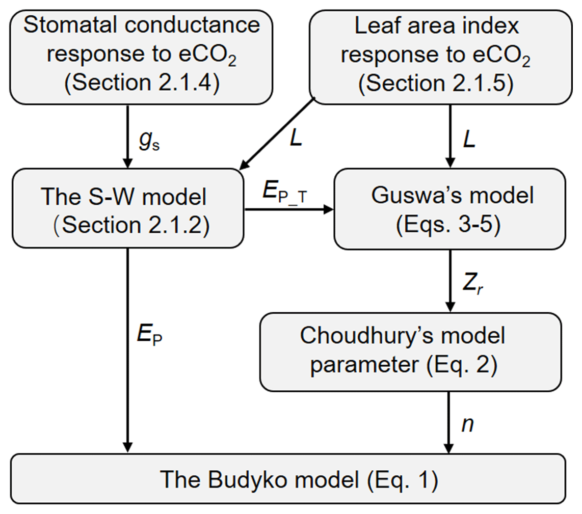
Figure 1Flowchart of using the analytical models to detect the eCO2 impact on Q. The terminologies used are explained in the following text (Sect. 2.1.1 through to 2.1.5).
2.1.1 Runoff simulation
The BCP model adopts the formulation of the Budyko curve by Choudhury (1999), which is given as
where E is the annual average actual evapotranspiration (mm yr−1). P is the annual average precipitation (mm yr−1). EP is the annual average potential evapotranspiration (mm yr−1) here estimated using the Shuttleworth–Wallace two-source evapotranspiration model (Shuttleworth and Wallace, 1985; see Sect. 2.1.2). n is a unitless model parameter that encodes all factors other than mean climate conditions and modifies the partitioning of P between E and Q. For assumed steady-state conditions, Q is calculated by subtracting E from P as a result of catchment water balance.
The probabilistic steady-state solution to the stochastic dynamic soil moisture model by Porporato (2004) shares a similar form with the Budyko curve (Porporato et al., 2004). Porporato's parameter ω is a dimensionless parameter, which is a function of effective rooting depth (Zr, mm), mean rainfall intensity (α, mm per event), and soil water holding capacity (WHC, mm3 mm−3), and it exhibits a close relationship with Choudhury's parameter n (Yang et al., 2016b; Porporato et al., 2004). A relationship between Porporato's ω parameter and Choudhury's n parameter was built following three steps. Firstly, we obtained the numerical solution of Porporato's model for the corresponding for every 0.1 increment in for six separate ω curves. Secondly, by numerically solving Choudhury's formulation of the Budyko curve, we determined the values of Choudhury's parameter (n) that correspond to the values of each of the six ω curves. Thirdly and finally, we pooled all n–ω pairs together and deduced the relationship between n and ω (R2=0.96, p < 0.001; Supplement Fig. S1) as
Effective rooting depth (Zr) was determined using an analytical carbon cost-benefit model based on ecosystem optimality theory proposed by Guswa (2008). The Zr model is given as
where W is the ratio of the multiyear growing season mean P over potential transpiration, EP_T; γr is the root respiration rate (g C g−1 roots d−1), which is quantified using the standard Q10 theory (Lloyd and Taylor, 1994; Ryan, 1991) with a fixed Q10 coefficient of 2.0 (Zhao et al., 2011). The base respiration rate at 20 ∘C for each biome type is determined following Heinsch (2003). RLD is the root length density (cm roots cm−3 soil), and SRL is the specific root length (cm roots g−1 roots). We fixed RLD to be 0.1 cm roots cm−3 soil and SRL to be 1500 cm roots g−1, representing the median value of these two parameters reported in the literature (Caldwell, 1994; Eissenstat, 1997; Fitter and Hay, 2002; Pregitzer et al., 2002). fGS is the fraction of the growing season within a year, with the growing season length quantified according to Zhu et al. (2016). WUE is the photosynthetic water use efficiency (g C cm−3 H2O), which is determined for the first period (i.e., 1982–1985) from the ensemble mean from eight ecosystem models (see Data section) of annual gross primary production (GPP) and transpiration (ET) estimates (i.e., WUE = GPP ET). For the following periods, WUE was estimated by considering the effects of changes in atmospheric CO2 concentration (Ca) and vapor pressure deficit (v) on WUE (Donohue et al., 2013; Wong et al., 1979; Farquhar et al., 1993) as
where t is time in year. Note that the above equation implicitly assumes the same upscaling factor when converting the leaf-level assimilation and transpiration to the canopy level for a given location (Donohue et al., 2017). The spatial pattern of mean annual Zr is shown in Supplement Fig. S2.
2.1.2 The Shuttleworth–Wallace model
The Shuttleworth–Wallace two-source evapotranspiration model (the S–W model) was used to estimate EP and its two components (potential transpiration, EP_T, and potential evaporation, EP_S) (Shuttleworth and Wallace, 1985). The S–W model estimates evapotranspiration as
where λ is the latent heat for vaporization (MJ kg−1), Δ is the gradient of the saturation vapor pressure with respect to temperature (kPa K−1), ρ is the air density (kg m−3), cp is the specific heat of air at constant pressure (MJ kg−1 K−1), γ is the psychrometric constant (kPa K−1). , , and are the aerodynamic resistance (s m−1) to heat and vapor transfer between the canopy–air space and the atmosphere, between the leaf and the canopy–air space, and between the soil surface and the canopy–air space, respectively. These three aerodynamic resistance terms are estimated following Sánchez et al. (2008). and are soil surface resistance and stomatal resistance (the reciprocal of stomatal conductance), respectively. To estimate EP using the S–W model, is set to zero, and is set to its non-water-stressed value (Milly and Dunne, 2016). The non-water-stressed values of for each biome type are provided in Mu et al. (2007). A is the available energy (equal to net radiation minus ground heat flux, W m−2), and As is the available energy at the soil surface, which is estimated as a function of L following Beer's law (Campbell and Norman, 1998; Yang and Shang, 2013). As a result, A – As is the available energy absorbed by the plant canopy. The impacts of eCO2 on EP and its two components are obtained by allowing L and to vary with Ca. Recently, Milly and Dunne (2016) showed that the S–W model could most satisfactorily reproduce evapotranspiration estimates under non-water-limited conditions from climate models under eCO2.
2.1.3 Attribution of runoff changes
We used the BCP model to attribute changes in Q (dQ) due to different influencing factors following Roderick and Farquhar (2011). To a first-order approximation, the change in Q (dQ) is
where , , and represent the sensitivity of Q to changes in P, EP, and n, respectively, and can be expressed as
The physiological (stomatal conductance, gs) and structural (leaf area index, L, and effective rooting depth, Zr) parameters impact both EP and n. More specifically, decreases in gs lower the transpiration rate per leaf area, whereas increases in L and Zr enhance the canopy-level transpiration rate. Additionally, increases in L also reduce soil evaporation by shading the soil surface (Shuttleworth and Wallace, 1985). The impact of eCO2 on parameter n is expressed through its impact on Zr. On the one hand, increases in WUE induced by eCO2 permit a larger vegetation carbon uptake per amount of water loss, potentially leading to more carbon allocated to roots and thus a deeper Zr. Conversely, increases in plant water demand (as quantified by potential transpiration) require vegetation to develop deeper roots to access deeper soil moisture and vice versa (Guswa, 2008). As a result, we write the functional dependencies of EP and Zr as
where EP_M is the meteorological component of EP (without considering the increases in Ca). O represents factors other than eCO2 that affect Zr, which effectively encode the climate-change-induced vegetation change. Functions f and g describe these relationships. Changes in EP and Zr are given by
Combining Eqs. (2), (15), (21), and (22), we have
The first term on the right-hand side of Eq. (23) represents dQ caused by P change, and the second term represents dQ caused by eCO2. The third term calculates dQ induced by changes in EP_M and is calculated as . The fourth and fifth terms on the right-hand side of Eq. (23) represent dQ caused by changes in rainfall intensity and climate-change-induced vegetation change, respectively, and we group them as one factor in the attribution of dQ. Since our primary focus was to examine how eCO2 affects vegetation and the consequent impact on Q, as well as its relative importance to changes in P and EP_M, the other factors driving dQ were estimated as the residual of Eq. (23) (i.e., total dQ minus the sum of dQ induced by dP, dEP_M, and eCO2). By introducing Eqs. (17) and (18) into Eq. (23), the sensitivity of Q to eCO2 (SQ_to_eCO2, mm yr−1 ppm−1) is written as
The sensitivities of EP and Zr to eCO2 (i.e., and ) are quantified by numerically running the EP model and Zr model with and without changes in Ca, respectively. The difference between the two simulations under the two Ca scenarios is considered the net effect of eCO2 on Q.
2.1.4 Stomatal conductance response to eCO2
The response of leaf-level stomatal conductance (gs) response to eCO2 was determined using 244 field experiments with artificially elevated CO2 across a broad range of bioclimates (Ainsworth and Rogers, 2007). We linearly rescaled the reported change in gs for the magnitude of eCO2 in each of the 244 studies to obtain the sensitivity of gs to eCO2, that is, the percentage change in gs per 1 % increase in Ca. We then classified the 244 observations based on their biome type to construct a biome-type-based look-up table of gs sensitivity to eCO2.
2.1.5 Resource availability index and L response to eCO2
The response of L to eCO2 was predicted based on the response of WUE to eCO2 adjusted by the local resource availability. We define a site resource availability index (β) based on growing season mean L following Donohue et al. (2017). This is because observed L at a site is the net response to the local growing conditions and provides an effective proxy of the growing conditions experienced by vegetation (Donohue et al., 2017). Another advantage of this approach is that L can be readily measured directly or remotely. We calculated β as
where τ is an exponential extinction coefficient, which typically varies from 0.3 to 1.2 (Campbell and Norman, 1998) and is set to be 0.7 herein. Broadly across the globe, β also corresponds well with climate aridity. The calculated β increases from 0.0 with low resource availability (typically dry and/or cold) to 1.0 with high resource availability (typically warm and humid) (Fig. 2). This suggests a predominant role of the climate in shaping the global vegetation pattern (Budyko, 1974; Nemani et al., 2003; Yang et al., 2015). This also implies that the resource limitations on plant growth are mainly exerted by climate, which is consistent with the framework of climate limitation on vegetation proposed in previous studies (Nemani et al., 2003; Budyko, 1974; Yang et al., 2015). Then following Norby and Zak (2011), who showed that the observed response of L to eCO2 was a nonlinear function of L, we estimated the relative change in L induced by eCO2 as per Donohue et al. (2017):
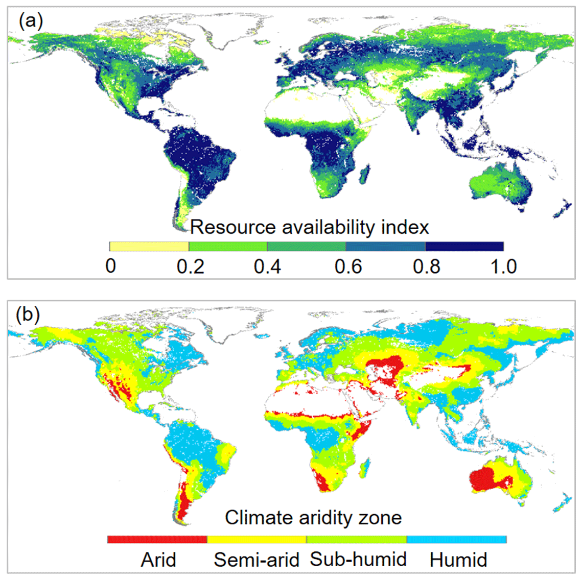
Figure 2Spatial distributions of (a) resource availability index categories and (b) climate aridity zones over global vegetated lands for 1982–2010. For the land surface, blank areas are non-vegetated regions. Respectively, there are 2536, 8194, 10316, 12930, and 9093 resolution grid cells in the 0.0–0.2, 0.2–0.4, 0.4–0.6, 0.6–0.8, and 0.8–1.0 resource availability index categories.
2.2 Data
The BCP model is validated against observed Q in 2268 strictly selected unimpaired catchments located across the globe that cover a broad range of bioclimates (Fig. 3). Originally, daily and/or monthly Q observations were collected from more than 22 000 catchments globally (Beck et al., 2019). Three selection criteria were implemented to ensure that only catchments with continuous Q records that are negligibly affected by humans were used. First, catchments with > 5 % missing data during the entire study period (1982–2010) were removed. Linear interpolation was applied to fill the gaps in the remaining Q series. Second, catchments smaller than 100 km2 were excluded. This is to ensure that at least one precipitation pixel (i.e., 0.1∘ × 0.1∘ or ∼ 100 km2) is included for a catchment. Third, we excluded catchments where observed Q is likely to be affected by human interventions, including catchments with (i) significant forest gain or loss (> 2 % of the total catchment area) (Hansen et al., 2013), (ii) irrigated areas larger than 2 % (Siebert et al., 2005), (iii) urban areas (https://www.edenextdata.com/?q=content/esa-globcover-version-23-2009-300m-resolution-land-cover-map-0, last access: 17 June 2019) larger than 2 %, and (iv) the presence of large dams (Lehner et al., 2011) (i.e., where the reservoir's capacity in a catchment is larger than 10 % of the catchment mean annual Q). Exactly 2268 catchments pass these selection criteria (Fig. 3).
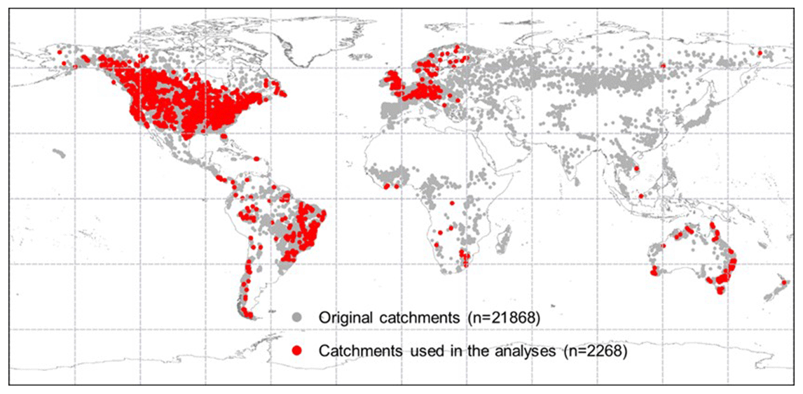
Figure 3Locations of the catchments across the globe. The grey dots show the locations of the original 21 856 catchments, and red dots are the 2268 catchments that pass the selection criteria and are used herein.
Precipitation from 1981 through 2010 was sourced from the Multi-Source Weighted-Ensemble Precipitation (MSWEP) version 2 dataset, which has a 3 h temporal resolution and 0.1∘ spatial resolution (Beck et al., 2019). The mean rainfall intensity was calculated as the ratio of annual total precipitation over the number of wet days (with daily precipitation higher than 1 mm; Hartmann et al., 2013). Other climate variables, including net radiation, air temperature, relative humidity, air pressure, and wind speed were obtained from the Multi-scale Synthesis and Terrestrial Model Intercomparison Project (MsTMIP; Wei et al., 2014). To obtain a spatial pattern of WUE, global monthly GPP and ET estimates over 1982–1985 were obtained from eight ecosystem models from MsTMIP (Huntzinger et al., 2013), including (i) CLM (Mao et al., 2012), (ii) CLM4-VIC (Li et al., 2011), (iii) ISAM (Jain et al., 1996), (iv) TRIPLEX (Peng et al., 2002), (v) LPJ-wsl (Sitch et al., 2003), (vi) ORCHIDEE-LSCE (Krinner et al., 2005), (vii) SiBCASA (Schaefer et al., 2008), and (viii) VISIT (Ito, 2010). Monthly Ca from 1982–2010 was obtained from the Hawaiian Mauna Loa Observatory (http://www.esrl.noaa.gov/gmd/obop/mlo/, last access: 30 June 2019), and we assume a uniform Ca concentration across the globe at the mean annual scale (i.e., 5 years). Monthly L for 1982–2010 was derived from Zhu et al. (2013) based on AVHRR GIMMS-3g NDVI data (Pinzon and Tucker, 2014). Land cover classification in the year 2001 was acquired from the Moderate Resolution Imaging Spectroradiometer (MODIS) land use map (MOD12Q1) available from the NASA Data Center (Friedl et al., 2010). The global C4 vegetation fraction was obtained from the International Satellite Land Surface Climatology Project (ISLSCP) Initiative II C4 Vegetation Percentage dataset (Still et al., 2009; http://webmap.ornl.gov/ogcdown/dataset.jsp?ds_id=932, last access: 24 June 2018). Soil texture data at 30′′ spatial resolution was acquired from the Harmonized World Soil Database (HWSD) (Nachtergaele et al., 2009), which was used to determine WHC according to the US Department of Agriculture (USDA) soil classification (Saxton and Rawls, 2006). For catchment-scale calculations, these gridded data were further aggregated for individual catchments at a mean annual scale (i.e., 5 years). For grid cell analyses, all gridded datasets were resampled to a 0.5∘ resolution.
3.1 Validation of the BCP model in runoff estimation
The validity of the BCP model is tested by comparing the estimated Q with observed Q, in terms of both spatial and temporal variability, at the 2268 unimpaired catchments (Fig. 4). Spatially, the BCP model well captures the observed spatial variability in Q at the mean annual scale, with a coefficient of determination (R2) of 0.93, root-mean-squared error (RMSE) of 87.9 mm yr−1, and mean bias (estimated Q minus observed Q) of −11.4 mm yr−1 (Fig. 4a). Temporally, trends in mean annual Q are also reasonably reproduced by the BCP model, having an R2 of 0.71, RMSE of 0.71 mm yr−2, and mean bias of −0.05 mm yr−2 (Fig. 4b). Additionally, we also perform a sensitivity analysis by comparing the simulated Q using the BCP model with and without considering eCO2. Results show that the BCP model, when considering eCO2, performed better in estimating Q trends than the BCP model without considering eCO2, as evidenced by an improvement of R2 by 0.02, a reduction of RMSE by 0.03 mm yr−2, and a decrease of mean bias by 0.11 mm yr−2, averaged over all 2268 catchments (Fig. 4d). More apparent improvements of the BCP model performance with the consideration of eCO2 are found in regions having a relatively higher resource availability index. For β of 0.4–0.6, 0.6–0.8, and 0.8–1.0, the mean bias of simulated Q trends with eCO2 is −0.02, 0.06, or −0.36 mm yr−2 but increased to 0.24, 0.20, or −0.53 mm yr−2, respectively, when eCO2 is not considered (Fig. 4d). These results suggest that the analytical framework developed herein captures the eCO2 signal on the observed Q changes.
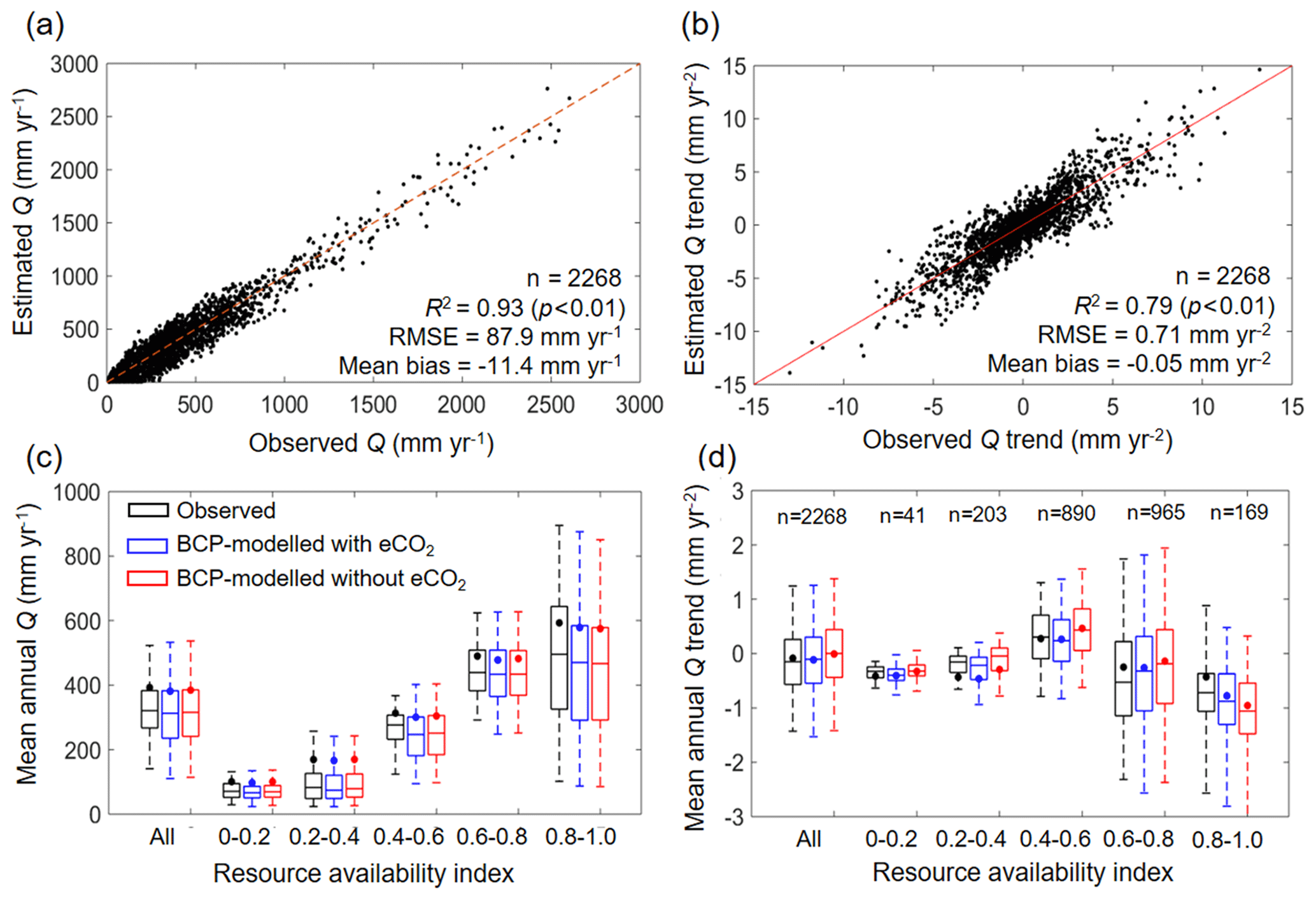
Figure 4Validation of estimated Q at catchments. (a) Model performance in predicting mean annual Q in 2268 catchments over 1982–2010. (b) Model performance in predicting Q trend in 2268 catchments during 1982–2010. (c) Model performance in predicting mean annual Q in 2268 catchments over 1982–2010 stratified by resource availability index category. (d) Model performance in predicting Q trend in 2268 catchments over 1982–2010 stratified by resource availability index category. The number of catchments in each resource availability index category are provided at the top of each subplot. The legend from (c) applies to (d). In (c) and (d), the upper and lower box edges represent the quartile division, the inner horizontal line is the median, the dots indicate the mean, and the dashed lines represent the 5th and 95th percentiles.
3.2 Plant physiological and structural responses to eCO2
The physiological response of plants to eCO2, that is, the response of gs to eCO2, is directly compiled from field experiments and summarized for each plant functional type in Ainsworth and Rogers (2007) (also see Supplement Fig. S3). All those field experiments report a reduction of gs in response to eCO2, with the largest gs reduction found in C4 crops and lowest in shrubs for the same level of eCO2. On average, for a 1 % increase in Ca, gs decreases by 0.47 % ± 0.12 % (mean ± 1 standard deviation), which means that gs decreases by 5.67 % ± 1.47 % under a 12.1 % increase in Ca over 1982–2010 (i.e., from ∼343.7 ppm in 1982–1985 to 385.2 ppm in 2006–2010; Keeling et al., 2001). This result is consistent with a recent isotope-based study (i.e., ∼ 5 % reduction of gs during the past 3 decades; Frank et al., 2015).
For structural response, averaged across global vegetated lands, our model reveals that elevated Ca has caused an increase of L by 2.12 % (0.14 % and 3.88 % for 5th and 95th percentiles) over 1982–2010 (Fig. 5a and b). Despite this relatively small fertilization effect of eCO2 on L at the global scale, an evident gradient is found in the L–eCO2 response: a larger eCO2-induced relative L increase is found in low resource availability regions (smaller β value in Fig. 2a) and vice versa (Fig. 5b). This modeled pattern of L–eCO2 response agrees very well with observations at the Free-Air CO2 Enrichment (FACE) observations (R2= 0.96, p < 0.01; Fig. 5c) and is also consistent with large-scale satellite-based observations (Donohue et al., 2013; Zhu et al., 2016; Yang et al., 2016a).
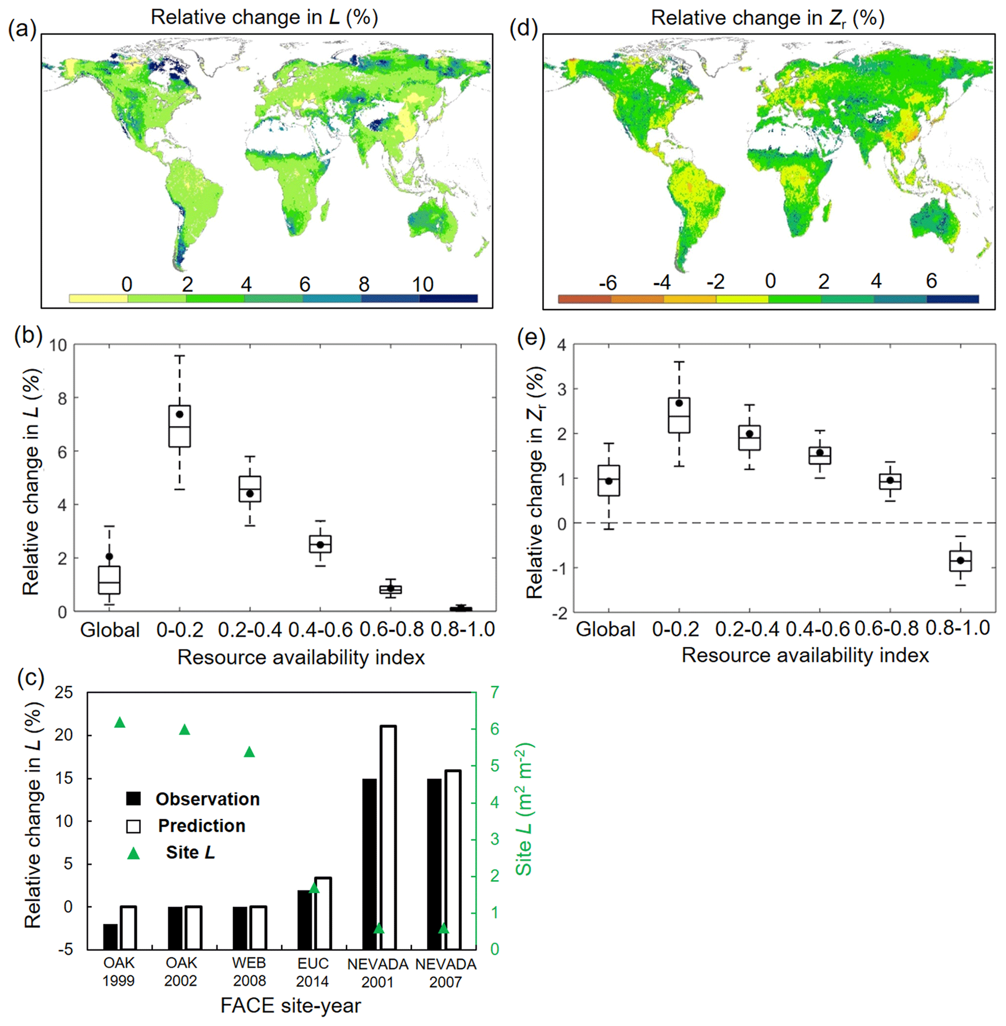
Figure 5Modeled relative changes in L and Zr caused by eCO2. (a) Spatial distribution of relative change in L induced by eCO2 during 1982–2010. (b) Same as (a) but for each resource availability index category. (c) Validation of predicted L change against in situ measurement during six Free-Air CO2 Enrichment (FACE) experiments. Note that only FACE sites with undisturbed vegetation are used (see Donohue et al., 2017). (d) Spatial distribution of relative change in Zr induced by eCO2 during 1982–2010. (e) Same as (d) but for each resource availability index category. In panels (b) and (e) the upper and lower box edges represent the quartile divisions, the inner horizontal line is the median, the dots indicate the mean, and the dashed lines represent the 5th and 95th percentiles. The number of grid cells in each resource availability index category is provided in Fig. 2.
In terms of Zr, our modeling results show that elevated Ca over 1982–2010 has resulted in a very minor (0.93 %, −0.12 % and 1.85 % for 5th and 95th percentiles) overall increase of Zr averaged across the globe (Fig. 5e). Since large-scale observations of Zr in response to eCO2 are not available, we are not able to quantitatively validate the estimated response of Zr to eCO2. Nevertheless, the modeled result that eCO2 increases Zr is overwhelmingly found in site- and/or plant-level experiments (Nie et al., 2013) (Tables S1 and S2). Moreover, similar to L, the response of Zr to eCO2 also exhibits a notable difference along the resource availability gradient (Fig. 5d and e). The positive response of Zr to eCO2 is larger in low-β regions and gradually decreases as the resource availability becomes higher. In high-β regions (e.g., tropical rainforest and Southeast Asia), Zr even shows a slight decrease in response to eCO2, suggesting a reduced plant water need given the range of Ca over 1982–2010 in those regions.
3.3 Attribution of runoff changes over 1982–2010
Over 1982–2010, Ca increased by ∼ 12.1 %. For the same period, the BCP model detected a very small reduction in Q of ∼ 1.7 % (or 2.2 mm yr−1) induced by eCO2 via vegetation feedbacks across the entire global vegetated lands (Figs. 6b and 7d). This 1.7 % reduction in Q, under the context of 12.1 % increases in Ca, demonstrates a muted response of Q to eCO2. In addition, the overall negative effect of eCO2 on Q suggests that the structural forcing of eCO2 on vegetation water consumption (both aboveground and belowground) outweighs the physiological effect of eCO2 driving leaf-level water saving. Across the global vegetated lands and for the same period, the physiological response of vegetation to eCO2 has led to an increased Q by 0.7 % (or 0.9 mm yr−1), with the simulated Q increases being increasingly larger as β increases (Fig. 6d). By contrast, the structural response of vegetation to eCO2 has resulted in an overall Q reduction by 2.4 % (or 3.1 mm yr−1), with the decreases in Q being increasingly smaller as β increases (Fig. 6e). These two opposite responses of vegetation water use to eCO2 along the resource availability gradient have led to a significant positive trend (p < 0.01) in the Q–eCO2 response along the resource availability gradient, from a negative response in low-β landscapes to a positive response in high-β landscapes (Fig. 6b). Nevertheless, an exception is found in extreme arid zones (i.e., when β < 0.1; Fig. 6b). This is because, in extremely dry areas, the availability of water defines the outcome, and the sensitivity of Q to any changes in land surface properties is very small (Donohue et al., 2013; Roderick et al., 2014).
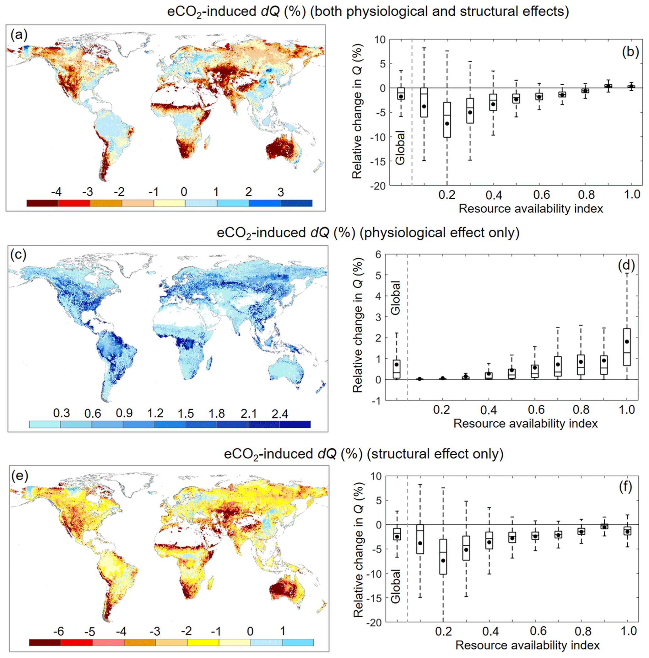
Figure 6Relative Q change induced by eCO2 during 1982–2010 across the global vegetated lands. (a) Spatial distribution of relative change in Q induced by eCO2. (b) Boxplot of relative change in Q induced by eCO2 for each resource availability index category. (c) Spatial distribution of relative change in Q induced by eCO2 when only the physiological effect is considered. (d) Boxplot of relative change in Q induced by eCO2 when only the physiological effect is considered for each resource availability index category. (e) Spatial distribution of relative change in Q induced by eCO2 when only the aboveground and belowground structural effects are considered. (f) Boxplot of relative change in Q induced by eCO2 when only the aboveground and belowground structural effects are considered for each resource availability index category. In (b), (d), and (f) the upper and lower box edges represent the quartile divisions, the inner horizontal line is the median, the dots indicate the mean, and the dashed lines represent the 5th and 95th percentiles. The number of grid cells in each resource availability index category is provided in Fig. 2.
We then attribute dQ to different forcing factors between 1982–1985 and 2006–2010 over the global vegetated lands (Figs. 7 and 8). Compared with the early 1980s (i.e., 1982–1985), mean observed Q over the global vegetated lands in the late 2010s (i.e., 2006–2010) increased by 29.7 mm yr−1, and the observed pattern with comparable magnitude in dQ is well captured by the BCP model (Fig. 4b and d). Consistent with relative Q changes (in %; Fig. 6), the impacts of eCO2 on the absolute Q change (in mm yr−1) also exhibit a significant upward trend as β increases (0.53 mm yr−1 per 0.1 increase in β, p < 0.01). Compared to that, increases in P led to a 43.9 mm yr−1 increase in Q, and enhanced EP_M has resulted in a decreased Q by 5.3 mm yr−1 (Fig. 7f). For the entire vegetated lands and each resource availability category, the impact of dP on Q generally dominates dQ and is often much higher than that of eCO2 (Fig. 7). An exception is the low-β regions (β < 0.2), where the impact of eCO2 on Q outweighs the impact of dP on Q (Fig. 8a). As for the impact EP_M on Q, it also shows a notable gradient with changes in β as detected for the eCO2 effect, with the impact of EP_M on Q being increasingly negative as β increases (Fig. 8b-e). The combined influence of other factors including changes in rainfall intensity (Porporato et al., 2004; Westra et al., 2013) and climate-change-induced vegetation change (e.g., higher L) have, in general, exerted a negative impact on Q.
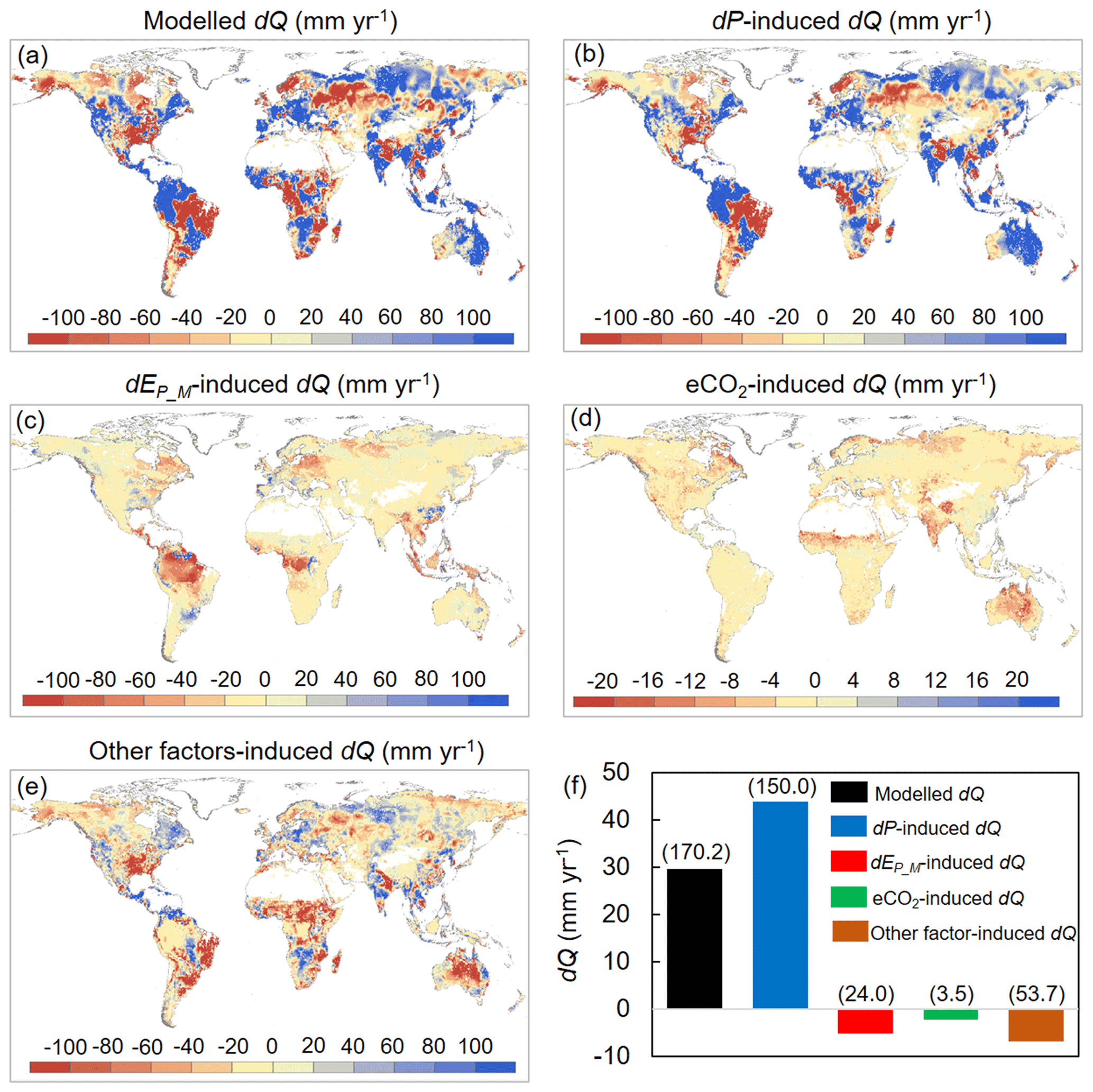
Figure 7Attribution of changes in Q between 1982–1985 and 2006–2010 across global vegetated lands. (a) Spatial distribution of changes in Q. (b–e) Spatial distributions of changes in Q induced by (b) changes in P, (c) changes in EP_M, (d) eCO2, and (e) changes in other factors (mainly rainfall intensity and climate-change-induced vegetation change). (f) Attribution of changes in Q between 1982–1985 and 2006–2010 averaged over the entire global vegetated lands. Values in parentheses represent 1 standard deviation of each response among all vegetated grid cells.
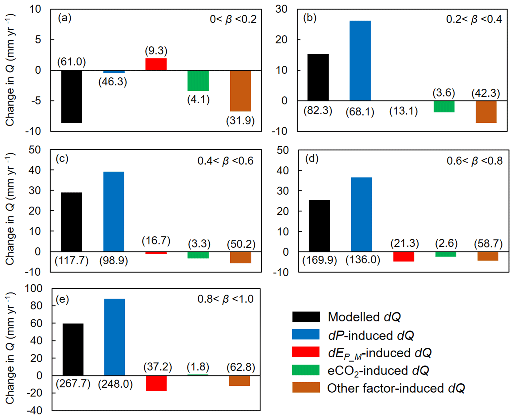
Figure 8Attribution of changes in Q between 1982–1985 and 2006–2010 at grid boxes within each resource availability index (β) category. Values in parentheses represent 1 standard deviation of each response among grid cells within each resource availability index category. The number of grid cells in each resource availability index category is provided in Fig. 2.
Since changes in meteorological factors (P and EP_M) are often considered to dominate changes in Q and have been extensively examined previously (e.g., Roderick and Farquhar, 2011; Yang et al., 2018; Zhang et al., 2018), we next examine the sensitivity of Q to eCO2 (SQ_to_eCO2) and compare it with the sensitivity of Q to changes in P and EP_M. Because Ca has different units from P and EP_M, we use relative units to better compare the three sensitivities (Fig. 9). Globally, an increase in Ca by 1 % only leads to a decrease of Q by ∼ 0.14 % (equivalent to ∼ 1.7 % for the range of eCO2 experienced over 1982–2010). Similar to the attribution results shown above (Fig. 6a and b), SQ_to_eCO2 is generally more negative in global arid ecosystems where β is low (Fig. 9a and b). The negative SQ_to_eCO2 diminishes quickly as β increases and becomes positive SQ_to_eCO2 in high-β regions. The overall small SQ_to_eCO2 is further manifested when comparing SQ_to_eCO2 with the sensitivities of Q to P and EP_M. Averaged across the global vegetated lands, the same relative change in P and EP would, respectively, lead to an ∼ 10 times and ∼ 4 times stronger impact on Q than eCO2 does. This highlights the predominant role of climate in shaping the global Q regime (Figs. 9c–f and S4).

Figure 9Sensitivity of Q to eCO2 and its relative importance to P and EP_M across the globe. (a) Spatial distribution of Q sensitivity to eCO2 (percent change in Q per 1 % change in Ca). (b) Boxplot of Q sensitivity to eCO2 for each resource availability index category. (c) Relative importance of eCO2 to Q compared to changes in P on Q (percent change in Q per 1 % change in Ca compared to percent change in Q per 1 % change in P). (d) Boxplot of the relative importance of eCO2 to Q compared to changes in P on Q for each resource availability category. (e) Relative importance of eCO2 toQ compared to changes in EP_M on Q (percent change in Q per 1 % change in Ca compared to percent change in Q per 1 % change in EP). (f) Boxplot of the relative importance of eCO2 to Q compared to changes in EP_M on Q for each resource availability category. In (b), (d), and (f), the upper and lower box edges represent the quartile divisions, the inner horizontal line is the median, the dots indicate the mean value, and the dashed lines represent the 5th and 95th percentiles. The number of grid cells in each resource availability index category is provided in Fig. 2.
Elevation in atmospheric CO2 concentration (and other greenhouses gases) is regarded as the ultimate driver of anthropogenic climate change, with consequent impacts on Q. Although the impacts of climate change on Q have been extensively studied, the response of Q to eCO2 through vegetation feedbacks is less understood and remains controversial (Gedney et al., 2006; Piao et al., 2007; Huntington, 2008; Cheng et al., 2014; Trancoso et al., 2017; Yang et al., 2016a; Ukkola et al., 2016a, b). Here, by developing an analytical attribution framework, we detected a very small response of global Q to eCO2-induced changes in vegetation structural (both aboveground and belowground) and physiological functioning (Figs. 6–8), suggesting that the eCO2 vegetation feedback only exerts a minor impact on water resources (partly due to the two opposing water effects between the structural and physiological responses to eCO2) for the range of eCO2 experienced over 1982–2010.
The overall negative impact of eCO2 on Q detected herein suggests that increased vegetation water consumption driven by the structural response of vegetation (i.e., increases in L and Zr) to eCO2 outweighs the functional change of leaf-level water saving caused by the physiological effect of eCO2 (i.e., decreases in gs). This result is consistent with previous findings by Cheng et al. (2014), Trancoso et al. (2017), and Ukkola et al. (2016a). In addition, we also detected a significant positive trend (p < 0.01) in the Q–eCO2 response along the resource availability gradient (Figs. 6–9). This Q–eCO2 response pattern suggests that the structural response of vegetation (i.e., increases in L and Zr) to eCO2 is larger in areas with lower resource availability and gradually decreases as resources become less limiting on plant growth (Fig. 5). The positive response of Q to eCO2 in high-β catchments (primarily located in tropical rainforests; Fig. 6a) implies a dominant effect of eCO2-induced partial stomatal closure over increases in L and Zr on E in these environments (Fig. 6). This is reasonable, as both theoretical predictions and in situ observations have consistently reported a negligible response of L to eCO2 in humid and closed-canopy environments (Donohue et al., 2017; Yang et al., 2016a; Norby and Zak, 2011; Körner and Arnone, 1992). In such environments, water is generally abundant with light and/or nutrient availability limiting vegetation growth (Nemani et al., 2003; Yang et al., 2015), and vegetation has evolved to efficiently capture light by maximizing its aboveground structure (i.e., L). As a result, in these high-L regions, vegetation has already absorbed most of the incident light, and any extra leaves would not materially increase the light absorption (Yang et al., 2016a). By contrast, in dry regions, an eCO2-induced increase in vegetation water use efficiency (so less transpiration for the same amount of carbon assimilation at the leaf level) would lead to an increase in L that is directly proportional to an increase in water use efficiency which would increase canopy-level carbon fixation (Fig. 5b). This finding is consistent with satellite observations (Donohue et al., 2013) and in situ FACE experiments (Norby and Zak, 2011).
Our findings have important implications for an improved understanding of the global hydrological cycle and managing the world's water resources in a changing climate. Climate models have predicted an increased Q that is primarily driven by an increased P for the 21st century (Lian et al., 2021; Milly and Dunne, 2016; Swann et al., 2016; Yang et al., 2018). Here we show that eCO2-induced vegetation feedbacks would mitigate this positive impact of climate change on Q in relatively dry regions and exacerbate the Q increase in relatively wet regions. In addition, higher Ca and increased P enhance the availability of resources for vegetation growth, which increases vegetation coverage or L (Piao et al., 2020; Zhang et al., 2020a, b). As the vegetation aboveground structural responses to eCO2 decrease with the increase of L, the predicted future L increases suggest that the structural response of vegetation to eCO2 may eventually decrease, and the physiological effect of vegetation on eCO2 may become increasingly dominant in the overall response of vegetation water use to eCO2, leading to an increasing water-saving effect of vegetation in response to eCO2 under future climate change (Zhang et al., 2020b). Analyses of the state-of-the-art climate model outputs already consistently show this water-saving effect of eCO2 globally, especially in relatively warm and humid environments where L is high (Yang et al., 2019). Nevertheless, this may partly be because only some climate models consider the physiological effect while ignoring structural responses of vegetation to eCO2. In addition, the impacts of eCO2 on Q in relatively dry regions are still highly uncertain and show a great diversity between climate models (Zhang et al., 2020b).
Finally, it is worthwhile noting that there are several limitations in the developed modeling framework. First, the rooting depth model by Guswa (2008) adopted herein employs an intensive root water uptake strategy, which assumes that root water uptake occurs at a potential rate (i.e., EP_T) until soil moisture reaches the wilting point when transpiration is completely suppressed (Guswa, 2008). This intensive root water uptake strategy differs from the root water uptake strategy employed in the stochastic soil water balance model by Porporato et al. (2004), which is a more conservative strategy under which root water uptake linearly decreases with the decrease of soil moisture (Porporato et al., 2004). Combining the two strategies into one modeling framework potentially leads to inconsistency in the theoretical aspect of the approach. In fact, a later study by Guswa (2010) incorporated the soil water balance model by Porporato et al. (2004) into Guswa's cost-benefit framework for rooting depth (referred to as the Guswa-2010 approach herein). However, the Guswa-2010 approach could not provide an explicit solution for Zr, because the solution for transpiration in Porporato's model is an incomplete gamma function of Zr (Guswa, 2010; Porporato et al., 2004). As a result, to allow an analytical solution to be derived, we used Guswa (2008) for Zr in our modeling framework. According to Guswa (2010), using the conservative root water uptake strategy resulted in a slightly deeper Zr compared to when the intensive strategy was used. Despite that, the response of Zr to changes in Ca under the two strategies should be similar, as the effects of eCO2 on Zr are expressed via water use efficiency and EP_T in our parameterization, which are independent of Zr parameterizations. This means that adopting different root water uptake strategies would only lead to differences in the resultant absolute magnitude of runoff (Q) but unlikely to result in differences in the response of Q to eCO2, especially when the relative magnitude is used (Figs. 5d, e and 6a, b, e and f). Alternatively, Rodríguez-Iturbe and Porporato (2004) incorporated the intensive root water uptake strategy into a stochastic soil water balance model and obtained a steady-state solution that has a simper form than the one by Porporato et al. (2004) and also mimics the Budyko curve. This approach deserves further investigation. Second, if interpreted strictly from a theoretical perspective, the model by Porporato et al. (2004) is more suitable to estimate hydrological partitioning during growing seasons instead of over the entire year as it assumes a constant evaporative demand and precipitation regimes and does not account for snow processes. Expanding all these simplifications and acknowledging imperfect knowledge and parameterization would require further analyses to better understand how they might affect the results shown here. Nevertheless, the uncertainties caused by these simplifications in the model by Porporato et al. (2004) might be partly overcome during the empirical connection made here between Porporato's model and Choudhury's formulation of the Budyko curve, as evidenced by the overall good performance of the developed BCP model in capturing the observed Q (Fig. 4). The third limitation of the current study lies in the steady-state assumption of the modeling framework. More specifically, the steady-state assumption is made in (i) catchment water balance and (ii) vegetation functioning. For point (i), a 5-year period does not necessarily guarantee zero-storage change. Nevertheless, the imbalance in water balance calculation under a steady-state assumption at a 5-year scale is generally very small (i.e., typically less than 6 % of P in arid regions and less than 3 % of P in humid regions) (Han et al., 2020). For point (ii), both Guswa's model for Zr and Donohue's model for L (see Sect. 2.1.5) adopted herein were developed for steady-state vegetation (i.e., mature and undisturbed vegetation). Applying these two models to immature (e.g., seedlings) and/or disturbed vegetation can be problematic, because immature and/or disturbed vegetation may have very different water use and carbon allocation strategies compared to steady-state vegetation (Donohue et al., 2017; Kuczera, 1987). However, the issues of vegetation age and disturbances are extremely complex and are well beyond our scope. Moreover, global datasets of vegetation age and disturbances are currently lacking. In this light, our modeled response of Q to eCO2 should be regarded as if all vegetation was mature and undisturbed. Further efforts are needed to better quantify the age and disturbances of vegetation and to better understand the water use and carbon allocation strategies through the entire vegetation life cycle and under various types of disturbances.
All data for this paper are properly cited and referred to in the reference list.
The supplement related to this article is available online at: https://doi.org/10.5194/hess-25-3411-2021-supplement.
YY and TRM designed the study. YY performed the calculation and drafted the article. TRM, DY, YZ, SP, SP, and HEB contributed to discussion of results and article writing.
The authors declare that they have no conflict of interest.
Tim R. McVicar acknowledges support from CSIRO Land and Water. The following organizations are thanked for providing observed streamflow data: the United States Geological Survey (USGS), the Global Runoff Data Centre (GRDC), the Brazilian Agência Nacional de Águas, the Water Survey of Canada (WSC), the Australian Bureau of Meteorology (BoM), and the Chilean Center for Climate and Resilience Research (CR2). Thanks to the Hydrology and Earth System Sciences editor and three anonymous reviewers for helpful comments that improved this study.
This research has been supported by the Ministry of Science and Technology of the People's Republic of China (grant no. 2019YFC1510604), the National Natural Science Foundation of China (grant nos. 42071029, 42041004), the Qinghai Department of Science and Technology (grant no. 2019-SF-A4), and the Guoqiang Institute of Tsinghua University (grant no. 2019GQG1020).
This paper was edited by Anke Hildebrandt and reviewed by three anonymous referees.
Ainsworth, A. E. and Rogers, A.: The response of photosynthesis and stomatal conductance to rising [CO2]: mechanisms and environmental interactions, Plant Cell Environ., 30, 258–270, https://doi.org/10.1111/j.1365-3040.2007.01641.x, 2007.
Beck, H. E., Wood, E. F., Pan, M., Fisher, C. K., Miralles, D. G., Van Dijk, A. I. J. M., McVicar, T. R., and Adler, R. F.: MSWEP V2 global 3-hourly 0.1∘ precipitation: methodology and quantitative assessment, B. Am. Meteorol. Soc., 3, 473–500, https://doi.org/10.1175/BAMS-D-17-0138.1, 2019.
Brown, A. E., Zhang, L., McMahon, T. A., Western, A. W., and Vertessy, R. A.: A review of paired catchment studies for determining changes in water yield resulting from alterations in vegetation, J. Hydrol., 310, 28–61, https://doi.org/10.1016/j.jhydrol.2004.12.010, 2005.
Budyko, M. I.: Climate and life, Academic, New York, USA, 1974.
Caldwell, M. M.: in Exploitation of Environmental Heterogeneity by Plants, Academic, San Diego, USA, 325–347, 1994.
Campbell, G. S. and Norman, J. M.: An Introduction to Environmental Biophysics, Springer, New York, USA, 1998.
Cheng, L., Zhang, L., Wang, Y. P., Yu, Q., Eamus, D., and O'Grady, A.: Impacts of elevated CO2, climate change and their interactions on water budgets in four different catchments in Australia, J. Hydrol., 519, 1350–1361, https://doi.org/10.1016/j.jhydrol.2014.09.020, 2014.
Choudhury, B.: Evaluation of an empirical equation for annual evaporation using field observations and results from a biophysical model, J. Hydrol., 216, 99–110, https://doi.org/10.1016/S0022-1694(98)00293-5, 1999.
Donohue, R. J., Roderick, M. L., and McVicar, T. R.: Roots, storms and soil pores: Incorporating key ecohydrological processes into Budyko's hydrological model, J. Hydrol., 436, 35–50, https://doi.org/10.1016/j.jhydrol.2012.02.033, 2012.
Donohue, R. J., Roderick, M. L., McVicar, T. R., and Farquhar, G. D.: Impact of CO2 fertilization on maximum foliage cover across the globe's warm, arid environments, Geophys. Res. Lett., 40, 3031–3035, https://doi.org/10.1002/grl.50563, 2013.
Donohue, R. J., Roderick, M. L., McVicar, T. R., and Yang, Y.: A simple hypothesis of how leaf and canopy-level transpiration and assimilation respond to elevated CO2 reveals distinct response patterns between disturbed and undisturbed vegetation, J. Geophys. Res.-Biogeo., 122, 168–184, https://doi.org/10.1002/2016JG003505, 2017.
Eissenstat, D. M.: in Ecology in Agriculture, edited by: Jackson, L. E., Academic, New York, USA, 173–199, 1997.
Farquhar, G. D., Lloyd, J., Taylor, J. A., Flanagan, L. B., Syvertsen, J. P., Hubick, K. T., Wong, S. C., and Ehleringer, J. R.: Vegetation effects on the isotope composition of oxygen in atmospheric CO2, Nature, 363, 439–443, 1993.
Fatichi, S., Leuzinger, S., Paschalis, A., Langley, J. A., Barraclough, A. D., and Hovenden, M. K.: Partitioning direct and indirect effects reveals the response of water-limited ecosystems to elevated CO2, P. Natl. Acad. Sci. USA, 113, 12757–12762, https://doi.org/10.1073/pnas.1605036113, 2016.
Field, C. B., Jackson, R. B., and Mooney, H. A.: Stomatal responses to increased CO2: implications from the plant to the global scale, Plant Cell Environ., 18, 1214–1225, https://doi.org/10.1111/j.1365-3040.1995.tb00630.x, 1995.
Fitter, A. H. and Hay, R. K. M.: Environmental Physiology of Plants, Academic, London, UK, 2002.
Frank, D. C., Poulter, B., Saurer, M., Esper, J., Huntingford, C., Helle, G., Treydte, K., Zimmermann, N. E., Schleser, G. H., Ahlstore, A., and Ciais, P.: Water-use efficiency and transpiration across European forests during the Anthropocene, Nat. Clim. Change, 5, 579–583, https://doi.org/10.1038/nclimate2614, 2015.
Friedl, M. A., Sulla-Menashe, D., Tan, B., Schneider, A., Ramankutty, N., Sibley, A., and Huang, X.: MODIS Collection 5 global land cover: Algorithm refinements and characterization of new datasets, Remote Sens. Environ., 114, 168–182, https://doi.org/10.1016/j.rse.2009.08.016, 2010.
Friedlingstein, P., Joel, G., Field, C. B., and Fung, I. Y.: Toward an allocation scheme for global terrestrial carbon models, Global Change Biol., 5, 755–770, https://doi.org/10.1046/j.1365-2486.1999.00269.x, 1999.
Gedney, N., Cox, P. M., Betts, R. A., Boucher, O., Huntingford, C., and Stott, P. A.: Detection of a direct carbon dioxide effect in continental river runoff records, Nature, 439, 835–838, https://doi.org/10.1038/nature04504, 2006.
Guswa, A. J.: The influence of climate on root depth: A carbon cost-benefit analysis, Water Resour. Res., 44, W02427, https://doi.org/10.1029/2007WR006384, 2008.
Guswa, A. J.: Effect of plant uptake strategy on the water-optimal root depth, Water Resour. Res., 46, W09601, https://doi.org/10.1029/2010WR009122, 2010.
Han, J. T., Yang, Y., Roderick, M. L., McVicar, T. R., Yang, D. W., Zhang, S. L., and Beck, H. E.: Assessing the steady-state assumption in water balance calculation across global catchments, Water Resour. Res., 56, e2020WR027392, https://doi.org/10.1029/2020WR027392, 2020.
Hansen, M. C., Potapov, P. V., Moore, R., Hancher, M., Turubanova, S. A., Tyukavina, A., Thau, D., Stehman, S. V., Goetz, S. J., Loveland, T. R., Kommareddy, A., Egorov, A., Chini, L., Justice, C. O., and Townshend, J. R. G.: High-Resolution Global Maps of 21st-Century Forest Cover Change, Science, 342, 850–853, https://doi.org/10.1126/science.1244693, 2013.
Hartmann, D. L., Klein Tank, A. M. G., Rusticucci, M., Alexander, L. V., Brönnimann, S., Charabi, Y., Dentener, F., Dlugokencky, E. J., Easterling, D. R., Kaplan, A., Soden, B. J., Thorne, P. W., Wild, M., and Zhai, P. M.: Observations: Atmosphere and Surface, in: Climate Change 2013: The Physical Science Basis, Contribution of Working Group I to the Fifth Assessment Report of the Intergovernmental Panel on Climate Change, edited by: Stocker, T. F., Qin, D., Plattner, G. K., Tignor, M., Allen, S. K., Boschung, J., Nauels, A., Xia, Y., Bex, V., and Midgley, P. M., Cambridge University Press, Cambridge, United Kingdom and New York, NY, USA, 2013.
Heinsch, F. A., Reeves, M., Votava, P., Kang, S., Cristina, M., Zhao, M., Glassy, J., Jolly, W. M., Loehman, R., Bowker, C. F., Kimball, J. S., and Nemani, R.: User's Guide GPP and NPP (MOD17A2/A3) Products NASA MODIS Land Algorithm, available at: https:////modis-land.gsfc.nasa.gov/pdf/MOD17UsersGuideV4.2June2019.pdf (last access: 15 June 2018), 2003.
Huntington, T. G.: Evidence for intensification of the global water cycle: Review and synthesis, J. Hydrol., 319, 83–95, https://doi.org/10.1016/j.jhydrol.2005.07.003, 2006.
Huntington, T. G.: CO2-induced suppression of transpiration cannot explain increasing runoff, Hydrol. Process., 22, 311–314, https://doi.org/10.1002/hyp.6925, 2008.
Huntzinger, D. N., Schwalm, C., Michalak, A. M., Schaefer, K., King, A. W., Wei, Y., Jacobson, A., Liu, S., Cook, R. B., Post, W. M., Berthier, G., Hayes, D., Huang, M., Ito, A., Lei, H., Lu, C., Mao, J., Peng, C. H., Peng, S., Poulter, B., Riccuito, D., Shi, X., Tian, H., Wang, W., Zeng, N., Zhao, F., and Zhu, Q.: The North American Carbon Program Multi-Scale Synthesis and Terrestrial Model Intercomparison Project – Part 1: Overview and experimental design, Geosci. Model Dev., 6, 2121–2133, https://doi.org/10.5194/gmd-6-2121-2013, 2013.
Ito, A.: Changing ecophysiological processes and carbon budget in East Asian ecosystems under near-future changes in climate: implications for long-term monitoring from a process-based model, J. Plant Res., 123, 577–588, https://doi.org/10.1007/s10265-009-0305-x, 2010.
Jain, A. K., Kheshgi, H. S., and Wuebbles, D. J.: A globally aggregated reconstruction of cycles of carbon and its isotopes, Tellus B, 48, 583–600, https://doi.org/10.1034/j.1600-0889.1996.t01-1-00012.x, 1996.
Keeling, C. D., Piper, S. C., Bacastow, R. B., Wahlen, M., Whorf, T. P., Heimann, M., and Meijer, H. A.: Exchanges of atmospheric CO2 and 13CO2 with the terrestrial biosphere and oceans from 1978 to 2000, I. Global aspects, SIO Reference Series No. 01–06, Scripps Institution of Oceanography, San Diego, USA, 88 pp., 2001.
Körner, C. and Arnone, J. A.: Responses to Elevated Carbon Dioxide in Artificial Tropical Ecosystems, Science, 257, 1672–1675, https://doi.org/10.1126/science.257.5077.1672, 1992.
Krinner, G., Viovy, N., Noblet-Ducoudré, N., Ogée, J., Polcher, J., Friedlingstein, P., Ciais, P., Sitch, S., and Prentice, C. I.: A dynamic global vegetation model for studies of the coupled atmosphere-biosphere system, Global Biogeochem. Cy., 19, GB1015, https://doi.org/10.1029/2003GB002199, 2005.
Kuczera, G.: Prediction of water yield reductions following a bushfire in ash-mixed species eucalypt forest, J. Hydrol., 94, 215–236, https://doi.org/10.1016/0022-1694(87)90054-0, 1987.
Lehner, B., Reidy, C., Revenga, L. C., Vörösmarty, C., Fekete, B., Crouzet, P., Döll, P., Endejan, M., Frenken, K., Magome, J., Nilsson, C., Robertson, J. C., Rödel, R., Sindorf, N., and Wisser, D.: High-resolution mapping of the world's reservoirs and dams for sustainable river-flow management, Front. Ecol. Environ., 9, 494–502, https://doi.org/10.1890/100125, 2011.
Li, H., Huang, M., Wigmosta, M. S., Ke, Y., Coleman, A. M., Leung, L. R., Wang, A., and Ricciuto, D. M.: Evaluating runoff simulations from the Community Land Model 4.0 using observations from flux towers and a mountainous watershed, J. Geophys. Res.-Atmos., 116, D24120, https://doi.org/10.1029/2011JD016276, 2011.
Lian, X., Piao, S. L., Chen, A. P., Huntingford, C., Fu, B. J., Li, Z. X., Huang, J. P., Sheffield, J., Berg, A. M., Keenan, T. F., McVicar, T. R., Wada, Y., Wang, X. H., Wang, T., Yang, Y. T., and Roderick, M. L.: Multifaceted characteristics of dryland aridity changes in a warming world, Nat. Rev. Earth Environ., 2, 232–250, https://doi.org/10.1038/s43017-021-00144-0, 2021.
Lloyd, J. and Taylor, J. A.: On the Temperature Dependence of Soil Respiration, Funct. Ecol., 8, 315–323, https://doi.org/10.2307/2389824, 1994.
Mao, J., Thornton, P. E., Shi, X., Zhao, M., and Post, W. M.: Remote Sensing Evaluation of CLM4 GPP for the Period 2000–2009, J. Climate, 25, 5327–5342, https://doi.org/10.1175/JCLI-D-11-00401.1, 2012.
Milly, P. C. D. and Dunne, K. A.: Potential evapotranspiration and continental drying, Nat. Clim. Change, 6, 946–949, https://doi.org/10.1038/nclimate3046, 2016.
Mu, Q., Zhao, M., and Running, S.: Improvements to a MODIS global terrestrial evapotranspiration algorithm, Remote Sens. Environ., 115, 1781–1800, https://doi.org/10.1016/j.rse.2011.02.019, 2007.
Nachtergaele, F., van Velthuizen, H., and Verelst, L.: Harmonized World Soil Database, FAO, Rome, Italy and IIASA, Laxenburg, Austria, 2009.
Nemani, R., Keeling, C. D., Hashimoto, H., Jolly, W. M., Piper, S. C., Tucker, C. J., Myneni, R. B., and Running, S. W.: Climate-Driven Increases in Global Terrestrial Net Primary Production from 1982 to 1999, Science, 300, 1560–1563, https://doi.org/10.1126/science.1082750, 2003.
Nie, M., Lu, M., Bell, J., Raut, S., and Pendall, E.: Altered root traits due to elevated CO2: a meta-analysis, Global Ecol. Biogeogr., 22, 1095–1105, https://doi.org/10.1111/geb.12062, 2013.
Norby, R. J. and Zak, D. R.: Ecological Lessons from Free-Air CO2 Enrichment (FACE) Experiments, Annu. Rev. Ecol. Evol. S., 42, 181–203, https://doi.org/10.1146/annurev-ecolsys-102209-144647, 2011.
Norby, R. J., Warren, J. M., Iversen, C. M., Medlyn, B. E., and McMurtrie, R. E.: CO2 enhancement of forest productivity constrained by limited nitrogen availability, P. Natl. Acad. Sci. USA, 107, 19368–19373, https://doi.org/10.1073/pnas.1006463107, 2010.
Oki, T. and Kanae, S.: Global Hydrological Cycles and World Water Resources, Science, 313, 1068–1072, https://doi.org/10.1126/science.1128845, 2006.
Peng, C., Liu, J., Dang, Q., Apps, M. J., and Jiang, H.: TRIPLEX: a generic hybrid model for predicting forest growth and carbon and nitrogen dynamics, Ecol. Model., 153, 109–130, https://doi.org/10.1016/S0304-3800(01)00505-1, 2002.
Piao, S., Friedlingstein, P., Ciais, P., Noblet-Ducoudre, N., Labat, D., and Zaehle, S.: Changes in climate and land use have a larger direct impact than rising CO2 on global river runoff trends, P. Natl. Acad. Sci. USA, 104, 15242–15247, https://doi.org/10.1073/pnas.0707213104, 2007.
Piao, S., Wang, X., Park, T., Chen, C., Lian, X., He, Y., Bjerke, J. W., Chen, A., Ciais, P., Tømmervik, H., Nemani, R. R., and Myneni, R. B.: Characteristics, drivers and feedbacks of global greening, Nat. Rev. Earth Environ., 1, 14–27, https://doi.org/10.1038/s43017-019-0001-x, 2020.
Pinzon, J. and Tucker, C. A.: Non-Stationary 1981–2012 AVHRR NDVI3g Time Series, Remote Sens.-Basel, 6, 6929–6960, https://doi.org/10.3390/rs6086929, 2014.
Porporato, A., Daly, E., and Rodriguez-Iturbe, I.: Soil Water Balance and Ecosystem Response to Climate Change, Am. Nat., 164, 625–632, https://doi.org/10.1086/424970, 2004.
Pregitzer, K. S., DeForest, J. L., Burton, A. J., Allen, M. F., Ruess, R. W., and Hendrick, R. L.: Fine Root Architecture of Nine North American Trees, Ecol. Monogr., 72, 293–309, https://doi.org/10.1890/0012-9615(2002)072[0293:FRAONN]2.0.CO;2, 2002.
Roderick, M. L. and Farquhar, G. D.: A simple framework for relating variations in runoff to variations in climatic conditions and catchment properties, Water Resour. Res., 47, W00G07, https://doi.org/10.1029/2010WR009826, 2011.
Roderick, M. L., Sun, F., Lim, W. H., and Farquhar, G. D.: A general framework for understanding the response of the water cycle to global warming over land and ocean, Hydrol. Earth Syst. Sci., 18, 1575–1589, https://doi.org/10.5194/hess-18-1575-2014, 2014.
Ryan, M. G.: The effects of climate change on plant respiration, Ecol. Appl., 1, 157–167, https://doi.org/10.2307/1941808, 1991.
Sánchez, J. M., Kustas, W. P., Caselles, V., and Anderson, M. C.: Modeling surface energy fluxes over maize using a two-source patch model and radiometric soil and canopy temperature observations, Remote Sens. Environ., 112, 1130–1143, https://doi.org/10.1016/j.rse.2007.07.018, 2008.
Saxton, K. E. and Rawls, W. J.: Soil Water Characteristic Estimates by Texture and Organic Matter for Hydrologic Solutions, Soil Sci. Soc. Am. J., 70, 1569–1578, https://doi.org/10.2136/sssaj2005.0117, 2006.
Schaefer, K., Collatz, G. J., Tans, P., Denning, A. S., Baker, I., Berry, J., Prihodko, L., Suits, N., and Philpott, A.: Combined Simple Biosphere/Carnegie-Ames-Stanford Approach terrestrial carbon cycle model, J. Geophys. Res.-Biogeo., 113, G03034, https://doi.org/10.1029/2007JG000603, 2008.
Shuttleworth, W. J. and Wallace, J. S.: Evaporation from sparse crops – an energy combination theory, Q. J. Roy. Meteor. Soc., 111, 839–855, https://doi.org/10.1002/qj.49711146910, 1985.
Siebert, S., Döll, P., Hoogeveen, J., Faures, J.-M., Frenken, K., and Feick, S.: Development and validation of the global map of irrigation areas, Hydrol. Earth Syst. Sci., 9, 535–547, https://doi.org/10.5194/hess-9-535-2005, 2005.
Sitch, S., Smith, B., Prentice, I. C., Arneth, A., Bondeau, A., Cramer, W., Kaplan, J. O., Levis, S., Lucht, W., Sykes, M. T., Thonicke, K., and Venevsky, S.: Evaluation of ecosystem dynamics, plant geography and terrestrial carbon cycling in the LPJ dynamic global vegetation model, Global Change Biol., 9, 161–185, https://doi.org/10.1046/j.1365-2486.2003.00569.x, 2003.
Sivapalan, M., Blöschl, G., Zhang, L., and Vertessy, R.: Downward approach to hydrological prediction, Hydrol. Process., 17, 2101–2111, https://doi.org/10.1002/hyp.1425, 2003.
Still, C. J., Berry, J. A., Collatz, G. J., and DeFries, R. S.: ISLSCP II C4 Vegetation Percentage, in: ISLSCP Initiative II Collection [Data set], edited by: Hall, F. G., Collatz, G., Meeson, B., Los, S., Brown de Colstoun, E., and Landis, D., National Laboratory Distributed Active Archive Center, Oak Ridge, Tennessee, USA, https://doi.org/10.3334/ORNLDAAC/932, 2009.
Swann, A. L. S., Hoffman, F. M., Koven, C. D., and Randerson, J. T.: Plant responses to increasing CO2 reduce estimates of climate impacts on drought severity, P. Natl. Acad. Sci. USA, 113, 10019–10024, https://doi.org/10.1073/pnas.1604581113, 2016.
Trancoso, R., Larsen, J. R., McVicar, T. R., Phinn, S. R., and McAlpine, C. A.: CO2-vegetation feedbacks and other climate changes implicated in reducing base flow, Geophys. Res. Lett., 44, 2310–2318, https://doi.org/10.1002/2017GL072759, 2017.
Ukkola, A. M., Prentice, I. C., Keenan, T. F., van Dijk, A. I. J. M., Viney, N. R., Myneni, R. B., and Bi, J.: Reduced streamflow in water-stressed climates consistent with CO2 effects on vegetation, Nat. Clim. Change, 6, 75–78, https://doi.org/10.1038/nclimate2831, 2016a.
Ukkola, A. M., Keenan, T. F., Kelley, D. I., and Prentice, I. C.: Vegetation plays an important role in mediating future water resources, Environ. Res. Lett., 11, 094022, https://doi.org/10.1088/1748-9326/11/9/094022, 2016b.
Wei, Y., Liu, S., Huntzinger, D. N., Michalak, A. M., Viovy, N., Post, W. M., Schwalm, C. R., Schaefer, K., Jacobson, A. R., Lu, C., Tian, H., Ricciuto, D. M., Cook, R. B., Mao, J., and Shi, X.: The North American Carbon Program Multi-scale Synthesis and Terrestrial Model Intercomparison Project – Part 2: Environmental driver data, Geosci. Model Dev., 7, 2875–2893, https://doi.org/10.5194/gmd-7-2875-2014, 2014.
Westra, S., Alexander, L. V., and Zwiers, F. W.: Global increasing trends in annual maximum daily precipitation, J. Climate, 26, 3904–3918, https://doi.org/10.1175/JCLI-D-12-00502.1, 2013.
Wong, S. C., Cowan, I. R., and Farquhar, G. D.: Stomatal conductance correlates with photosynthetic capacity, Nature, 282, 424–426, https://doi.org/10.1038/282424a0, 1979.
Yang, Y. and Shang, S.: A hybrid dual-source scheme and trapezoid framework-based evapotranspiration model (HTEM) using satellite images: Algorithm and model test, J. Geophys. Res.-Atmos., 118, 2284–2300, https://doi.org/10.1002/jgrd.50259, 2013.
Yang, Y., Randall, R. J., McVicar, T. R., and Roderick, M. L.: An analytical model for relating global terrestrial carbon assimilation with climate and surface conditions using a rate limitation framework, Geophys. Res. Lett., 42, 9825–9835, https://doi.org/10.1002/2015GL066835, 2015.
Yang, Y., Donohue, R. J., McVicar, T. R., Roderick, M. L., and Beck, H. E.: Long-term CO2 fertilization increases vegetation productivity and has little effect on hydrological partitioning in tropical rainforests, J. Geophys. Res.-Biogeo., 121, 2125–2140, https://doi.org/10.1002/2016JG003475, 2016a.
Yang, Y., Donohue, R. J., and McVicar, T. R.: Global estimation of effective plant rooting depth: Implications for hydrological modeling, Water Resour. Res., 52, 8260–8276, https://doi.org/10.1002/2016WR019392, 2016b.
Yang, Y., Zhang, S., McVicar, T. R., Beck, H. E., Zhang, Y. Q., and Liu, B.: Disconnection Between Trends of Atmospheric Drying and Continental Runoff, Water Resour. Res., 54, 4700–4713, https://doi.org/10.1029/2018WR022593, 2018.
Yang, Y., Roderick, M. L., Zhang, S., McVicar, T. R., and Donohue, R. J.: Hydrologic implications of vegetation response to elevated CO2 in climate projections, Nat. Clim. Change, 9, 44–48, https://doi.org/10.1038/s41558-018-0361-0, 2019.
Zhang, C., Yang, Y., Yang, D., Wang, Z. R., Wu, X., Zhang, S. L., and Zhang, W. J.: Vegetation response to elevated CO2 slows down the eastward movement of the 100th meridian, Geophys. Res. Lett., 47, e2020GL089681, https://doi.org/10.1029/2020GL089681, 2020a.
Zhang, C., Yang, Y., Yang, D., and Wu, X.: Multidimensional assessment of global dryland changes under future warming in climate projections, J. Hydrol., 592, 125618, https://doi.org/10.1016/j.jhydrol.2020.125618, 2020b.
Zhang, S., Yang, Y., McVicar, T. R., and Yang, D.: An Analytical Solution for the Impact of Vegetation Changes on Hydrological Partitioning Within the Budyko Framework, Water Resour. Res., 54, 519–537, https://doi.org/10.1002/2017WR022028, 2018.
Zhao, M. S., Running, S., Heinsch, F. A., and Nemani, R.: MODIS-Derived Terrestrial Primary Production, in: Land Remote Sensing and Global Environmental Change: NASA's Earth Observing System and the Science of ASTER and MODIS, Remote Sensing and Digital Image Processing, edited by: Ramachandran, B., Justice, B., Abrams, C. O., and Michael, J., Springer, 635–660, available at: https://www.fs.usda.gov/treesearch/pubs/39324 (last access: 15 June 2019), 2011.
Zhu, Z., Bi, J., Pan, Y., Ganguly, S., Anav, A., Xu, L., Samanta, A., Piao, S., Nemani, R., and Myneni, R. B.: Global Data Sets of Vegetation Leaf Area Index (LAI)3g and Fraction of Photosynthetically Active Radiation (FPAR)3g Derived from Global Inventory Modeling and Mapping Studies (GIMMS) Normalized Difference Vegetation Index (NDVI3g) for the Period 1981 to 2011, Remote Sens.-Basel, 5, 927–948, https://doi.org/10.3390/rs5020927, 2013.
Zhu, Z., Piao, S., Myneni, R. B., Huang, M., Zeng, Z., Canadell, J. G., Ciais, P., Sitch, S., Friedlingstein, P., Arneth, A., Cao, C., Cheng, L., Kato, E., Koven, C., Li, Y., Lian, X., Liu, Y., Liu, R., Mao, J., Pan, Y., Peng, S., Peñuelas, J., Poulter, B., Pugh, T., Stocker, B. D., Viovy, N., Wang, X., Wang, Y., Xiao, Z., Yang, H., Zaehle, S., and Zeng, N.: Greening of the Earth and its drivers, Nat. Clim. Change, 6, 791–795, https://doi.org/10.1038/nclimate3004, 2016.