Estimation of groundwater recharge from groundwater levels using nonlinear transfer function noise models and comparison to lysimeter data

The estimation of groundwater recharge is of paramount importance to assess the sustainability of groundwater use in aquifers around the world. Estimation of the recharge flux, however, remains notoriously difficult. In this study the application of nonlinear transfer function noise (TFN) models using impulse response functions is explored to simulate groundwater levels and estimate groundwater recharge. A nonlinear root zone model that simulates recharge is developed and implemented in a TFN model and is compared to a more commonly used linear recharge model. An additional novel aspect of this study is the use of an autoregressive–moving-average noise model so that the remaining noise fulfills the statistical conditions to reliably estimate parameter uncertainties and compute the confidence intervals of the recharge estimates. The models are calibrated on groundwater-level data observed at the Wagna hydrological research station in the southeastern part of Austria. The nonlinear model improves the simulation of groundwater levels compared to the linear model. The annual recharge rates estimated with the nonlinear model are comparable to the average seepage rates observed with two lysimeters. The recharges estimates from the nonlinear model are also in reasonably good agreement with the lysimeter data at the smaller timescale of recharge per 10 d. This is an improvement over previous studies that used comparable methods but only reported annual recharge rates. The presented framework requires limited input data (precipitation, potential evaporation, and groundwater levels) and can easily be extended to support applications in different hydrogeological settings than those presented here.

1 Introduction

Despite ongoing scientific efforts, the estimation of groundwater recharge remains a notoriously difficult task for hydrologists (e.g., Bakker et al., 2013). From the many techniques available (see, e.g., Healy and Scanlon, 2010, for an overview), methods using groundwater-level observations as the primary source of information are among the most popular. This is likely due to the abundance of available groundwater-level data and the simplicity of the methods (Healy and Cook, 2002). A well-known example is the water table fluctuation (WTF) method, which only requires an estimate of the specific yield and groundwater-level data as model input. An additional advantage of the WTF method is that no assumptions are made about the actual recharge processes, for example, the existence of preferential flow paths. This can also be considered a disadvantage, as no relationship between precipitation and recharge is established. This makes the method unsuitable for future projections of groundwater recharge when precipitation patterns change, for example, in climate change impact studies.

In a review paper on the topic, Healy and Cook (2002) suggested that “approaches based on transfer function noise (TFN) models should be further explored” for the estimation of recharge. TFN models can be used to translate one or more input series (e.g., precipitation and potential evaporation) into an output series (e.g., groundwater levels) and have been adopted in many branches of hydrology (Hipel and McLeod, 1994). An early example of the use of these models for recharge estimation is given in Besbes and De Marsily (1984), through the deconvolution of groundwater levels with an aquifer unit hydrograph obtained from a groundwater model. The study showed how the recharge flux can be related to rainfall by using an additional unit hydrograph for the unsaturated zone. Their proposed method required a calibrated groundwater model and a good estimate of the infiltration, making the method relatively laborious and less applicable in practice. O'Reilly (2004) developed a water balance–transfer function model to simulate recharge, using the WTF method to obtain recharge estimates to calibrate the model parameters.

In recent decades, the use of a specific type of TFN models using predefined impulse response functions (von Asmuth et al., 2002) has gained popularity for the analysis of groundwater levels. In this data-driven method, impulse response functions are used to describe how groundwater levels react to different drivers such as precipitation, evaporation, and pumping. The method has been successfully applied to characterize and analyze groundwater systems around the world, for example in Brazil (Manzione et al., 2010), Italy (Fabbri et al., 2011), the United Kingdom (Ascott et al., 2017), and India (van Dijk et al., 2019). The advantages of data-driven models compared to numerical groundwater models are faster model development and a lower number of calibration parameters (e.g., Bakker and Schaars, 2019). A large number of time series may be analyzed in a timely manner, for example, to improve the understanding of a groundwater system. Results are often also useful for the development of numerical groundwater models.

An important goal for these models has traditionally been to accurately describe observed groundwater-level fluctuations. For shallow water tables (up to a few meters' depth), this can often be achieved using a linear model between precipitation and evaporation on the one hand and groundwater levels on the other hand; i.e., when the rainfall doubles, so does the increase in the groundwater levels (e.g., Berendrecht et al., 2003; von Asmuth et al., 2008). In a large-scale case study for the Netherlands, Zaadnoordijk et al. (2019) obtained good results with this method for areas with shallow groundwater depths. For the simulation of deeper groundwater levels, the linear model was shown to be less appropriate, and nonlinear models may be used to accurately simulate the groundwater levels (e.g., Berendrecht et al., 2006; Peterson and Western, 2014; Shapoori et al., 2015). Such nonlinear models improve the simulation of groundwater levels by taking the nonlinear processes that occur in the root zone into account, for example, through the limitation of evaporation due to low soil moisture levels and the temporal storage of water within the root zone.

More recently, efforts have been made to explore the use of TFN models to estimate groundwater recharge, as suggested by Healy and Cook (2002). Hocking and Kelly (2016) constructed TFN models that included rainfall, evaporation, river levels, pumping, and a linear trend as explanatory variables, to isolate the contribution of rainfall to the groundwater-level fluctuations. This contribution was then converted to recharge using the hydrograph fluctuation method (Viswanathan, 1984). Obergfell et al. (2019) used a linear model to estimate average diffuse recharge and obtained good annual recharge estimates when compared to results from a chloride mass balance. Recognizing the importance of evaporation in their model setup, they constrained the parameter estimation by including the correct simulation of the seasonal behavior in the objective function. Peterson and Fulton (2019) used a nonlinear TFN model that includes a soil moisture module to estimate recharge (Peterson and Western, 2014). To obtain reasonable estimates of recharge, the model was constrained by comparing the modeled evaporation to the expected actual evaporation obtained using the Budyko curve. All of these studies reported annual recharge rates, but at least the latter method could in principle also be used to obtain estimates at smaller timescales.

In this study, exploration of the use of nonlinear TFN models using impulse response functions is continued to estimate groundwater recharge and improve the simulation of groundwater levels. A nonlinear recharge model is developed based on a soil-water storage approach and implemented in a TFN model to simulate the (nonlinear) effect of precipitation and evaporation on the groundwater levels. This study focuses on the estimation of recharge for relatively shallow groundwater systems without capillary rise of groundwater to the unsaturated zone. The estimated recharge fluxes are compared to long-term recharge rates measured with two lysimeters located at the hydrological research site Wagna in Austria, providing a unique opportunity to evaluate the recharge estimates at smaller timescales. Additionally, this study documents the extension of the commonly used autoregressive model with a moving-average part to model the residuals and obtain an approximately white noise series used for model calibration. The purpose of this study is to provide a proof-of-concept of the proposed methods through a detailed case study for a single location. The data from the lysimeters are only used to evaluate the model results and are not used to improve the results during model setup and calibration.

The next section provides an overview of the study site and the data used for model input and evaluation. In the third section, the methodological approach is described, starting with a brief overview of TFN modeling, followed by a description of the recharge models, and ending with a description of the model calibration. The results are presented and discussed in the fourth section, followed by a general discussion of the methodology in the fifth section. The conclusions of this study are summarized, and recommendations for future research are provided in the sixth and final section.

2 Study site and field data

The study site is the hydrological research station near the town of Wagna in Styria, Austria (see Fig. 1). The site is located in an agricultural field surrounded by residential areas. Groundwater levels have been observed with a daily time step since 1992 (see Fig. 2d; only data from 2006 onwards are shown here). The depth to water table is approximately 4 m, and no capillary rise of moisture from the water table into the root zone is expected due to the existence of a coarse gravel layer at a depth of 0.50–120 cm (Klammler and Fank, 2014). The land surface is at 267 m above mean Adriatic sea level (a.m.s.l.) with little elevation differences and small hydraulic head gradients (±2.5 m km⁻¹). The nearest drainage features are the Sulm River 1 km to the west and the larger Mur River 1.5 km to the east. Groundwater pumping for drinking water purposes occurs 500 m north of the observation well at a rate of 240 m³d⁻¹. Due to the low discharge and high conductivity of the aquifer, the effect of this pumping is assumed to be negligible at the study site. Given these conditions, the groundwater-level fluctuations are assumed to be the exclusive result of changes in the groundwater recharge from infiltrating precipitation water.

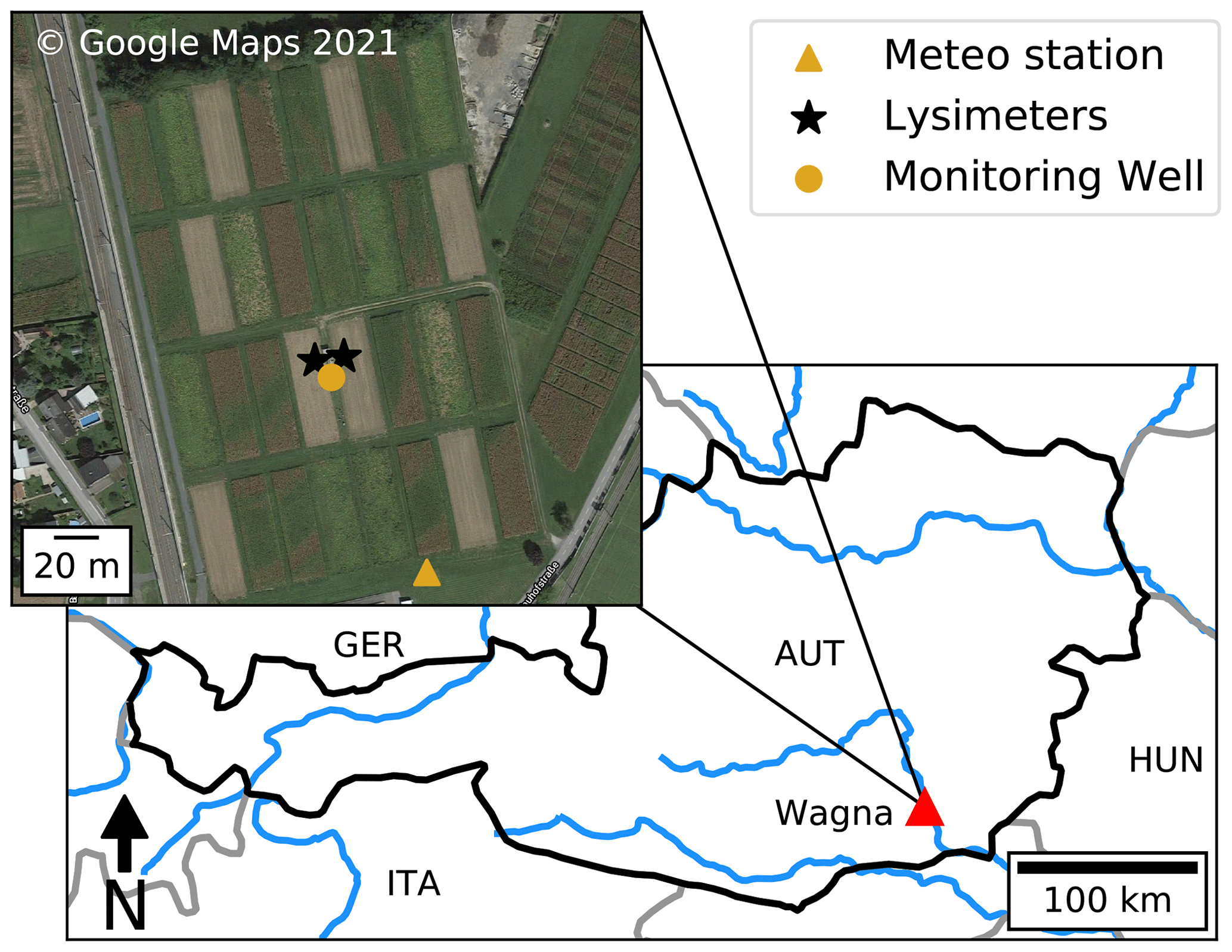
Figure 1 Map of the case study area with the locations of the lysimeters, the meteorological station, and the groundwater monitoring well used in this study.

The climate at the study area is influenced by the Mediterranean Sea in the south, the land masses of Hungary in the east, and the Alps in the west. The average air temperature is 18.6 ^∘C in summer (June–August) and −0.9 ^∘C in winter (December–February) (Prettenthaler et al., 2010). In the summer months there are approximately 8 to 9 h sunshine per day, while during the winter months the number of hours with sun averages only 2 to 3 h. Precipitation primarily occurs as short-duration convective rainfall events during the warm summer months. In winter, most of the precipitation also takes place as rainfall; the number of days with snowfall averages only 10 d yr⁻¹ (Prettenthaler et al., 2010). As the number of days when snowfall occurs is rather limited, the effect of snow on groundwater recharge is not taken into account in this study.

All the required input time series are measured directly at the site. This includes the precipitation and the meteorological variables required to calculate potential evaporation. It is noted here that the term “evaporation” rather than “evapotranspiration” is used throughout this paper (e.g., Savenije, 2004; Miralles et al., 2020). The FAO Penman–Monteith method is used to compute the daily grass reference evaporation (Allen et al., 1998). Klammler and Fank (2014) and Schrader et al. (2013) showed that the estimates from this method are in good agreement with estimates obtained from a grass lysimeter that is present at the site. The average annual precipitation (P) and grass reference evaporation (E_p) in the period 2007–2019 were 956 and 765 mm yr⁻¹, respectively. The time series of both fluxes are shown in Fig. 2a and b.

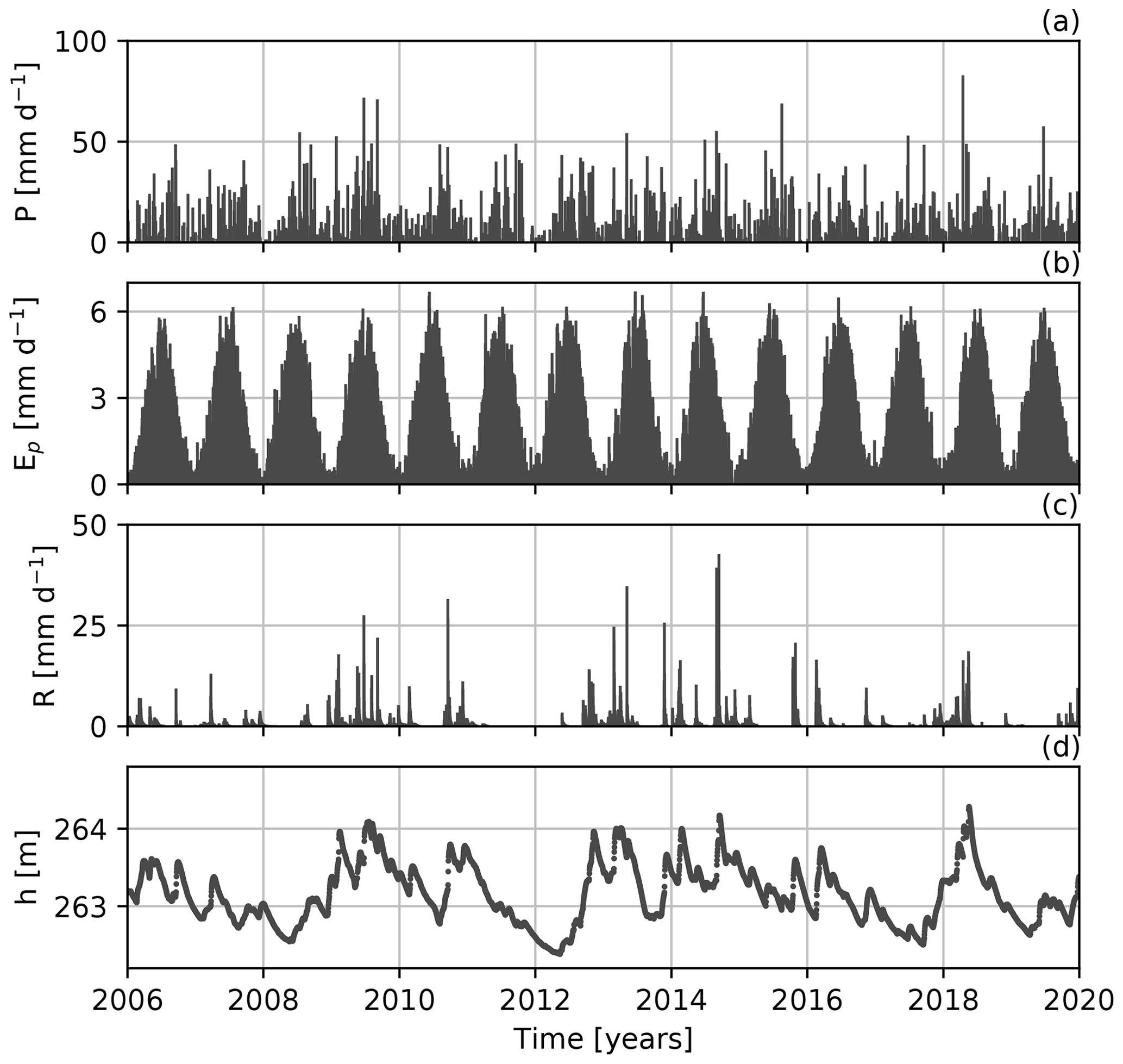
Figure 2 Time series of the precipitation (P), potential evaporation (E_p), recharge (R), and observed groundwater levels (h) for the period 2006 to 2020. The recharge shown here is the average seepage measured with the two lysimeters.

The study site is equipped with two weighable scientific field lysimeters, operated by JR-AquaConSol since 2005 (von Unold and Fank, 2008). The first lysimeter is operated under conventional farming practices (Sciencelys 1), while the second lysimeter (Sciencelys 2) was organically farmed until 2014, when it was also converted to conventional farming. A crop-rotation scheme is used for the lysimeters, with crops changing every growing season. The soils in the area are rather heterogeneous, with the thickness of the sandy loamy top layer varying greatly over short distances. The underlying sand and gravel deposits start at a depth between 50–120 cm. Both lysimeters have an area of 1 m² and are 2 m deep. Seepage to the groundwater is measured near the bottom of the lysimeters at 1.8 m depth, where suction cups are installed that apply a water potential that is similar to the potential measured with tensiometers just outside the lysimeters. Both lysimeters are identical in their technical setup, and a detailed description of the lysimeters is provided in von Unold and Fank (2008) and Klammler and Fank (2014).

As the recharge is not measured at the water table itself, a certain time lag between the recharge measured with the lysimeters and the corresponding groundwater-level rise exists. Only a limited time lag is expected as the ±2 m thick percolation zone consists mostly of highly conductive gravel layers. It is noted that the recharge measurements are local measurements for the area of the lysimeter and are influenced by prevailing soil conditions, vegetation, and the degree of soil sealing. The groundwater levels, measured at approximately 12 m distance from the lysimeters at the Wagna test site, may also be influenced by different recharge rates from other land-use types in the surrounding area (e.g., grassland or residential areas). As such, the measured recharge rates from the lysimeters are – for the purpose of this paper – used as an indicative rather than an exact estimate of recharge. Considering the above, the average recharge from the two lysimeters (shown in Fig. 2c) is used in this study for the comparison with model estimates. The average recharge measured with the lysimeters is 322 mm yr⁻¹ over the period 2007–2019.

A number of studies have used the hydrological research site Wagna. Only the literature with a focus on recharge estimation and unsaturated flow modeling is discussed here. Fank (1999) used the water table fluctuation method to estimate groundwater recharge from observed groundwater levels and computed an average recharge of 393 mm yr⁻¹ over the period 1992–1996. This estimate is comparable to the 296 and 396 mm yr⁻¹ reported by Stumpp et al. (2009) for the two lysimeters that were operated at the site in the period 1992–2001. Stumpp et al. (2009) also applied a HYDRUS-1D model to simulate unsaturated zone flow. Using stable isotope δ¹⁸O measurements, it was shown that lysimeter recharge could be adequately simulated with this physically based model, although recharge peaks were generally underestimated. Groenendijk et al. (2014) documented a large comparative study of six different unsaturated zone models, where measured water content and fluxes were used to calibrate and evaluate the models. Although this study focused on nitrate leaching, the study also showed how all models had difficulties in accurately simulating the water content and fluxes observed in the current lysimeters. This was attributed to the lack of processes such as hysteresis, preferential flow and multiple phase flow in the models. A later study using the MIKE SHE model yielded similar results (Reszler and Fank, 2016). The study concluded that the seepage and water content dynamics in the lower gravel zone inside the lysimeters could not be matched using the Richards equation and a Van Genuchten–Mualem approach, suggesting the existence of preferential flow paths below the root zone.

3 Methodology

3.1 The basic model setup

Transfer function noise (TFN) models are used here to translate recharge into groundwater levels. The basic model structure is

$$\begin{array}{}\text{(1)}& h\left(t\right)=h_{\mathrm{r}}\left(t\right)+d+r\left(t\right),\end{array}$$

where h(t) [L] are the observed groundwater levels, d [L] is the base level of the model, h_r(t) [L] is the contribution of the recharge to groundwater-level fluctuations, and r(t) [L] are the model residuals. The contribution h_r(t) [L] is computed by convoluting a recharge flux R(t) [L T⁻¹] with a predefined impulse response function θ(t) (von Asmuth et al., 2002):

$$\begin{array}{}\text{(2)}& h_{\mathrm{r}}\left(t\right)=\underset{-\mathrm{\infty }}{\overset{t}{\int }}R\left(\mathit{\tau }\right)\mathit{\theta }(t-\mathit{\tau })d\mathit{\tau }.\end{array}$$

Following Bakker et al. (2008), a four-parameter impulse response function is used to translate the recharge flux into groundwater-level fluctuations:

$$\begin{array}{}\text{(3)}& {\mathit{\theta }}_f\left(t\right)=A{t}^{n-\mathrm{1}}{\text{e}}^{-t/a-ab/t}t\ge \mathrm{0},\end{array}$$

where A [T${}^{-n+\mathrm{1}}$] is a scaling parameter, and a [T], b [–], and n [–] are shape parameters. For n>1, the four-parameter function simulates a delayed response of the groundwater levels to recharge, while for n≤1 and b=0, the groundwater levels respond instantaneously to a recharge pulse. If n=1 and b=0, Eq. (3) reduces to an exponential response function with only two parameters:

$$\begin{array}{}\text{(4)}& {\mathit{\theta }}_e\left(t\right)=A{\text{e}}^{-t/a}t\ge \mathrm{0}.\end{array}$$

The parameters A, a, n, b, and d are estimated by fitting Eq. (1) to observed data. Depending on the hydrogeological setting and the model used to compute the recharge, either a four-parameter or an exponential response function is used here to translate the recharge flux R into groundwater-level fluctuations. The main question that remains is how to estimate the recharge R(t) from observed hydrometeorological data. The following two sections introduce the two models used in this study to compute the recharge flux R(t).

3.2 The linear model

A common approach to approximate the recharge flux R in Eq. (2) is a simple linear function of precipitation P [L T⁻¹] and potential evaporation E_p [L T⁻¹] (e.g., Berendrecht et al., 2003; von Asmuth et al., 2008):

$$\begin{array}{}\text{(5)}& R=P-f{E}_{\mathrm{p}},\end{array}$$

where f [–] is a parameter that is calibrated. The grass reference evaporation computed using the Penman–Monteith equation (Allen et al., 1998) is used as potential evaporation E_p here. A clear interpretation of the parameter f is not available. While Berendrecht et al. (2003) referred to f as a crop factor, von Asmuth et al. (2008) noted that the value of f “depends on the soil and land cover” instead of a single crop and also incorporates the “average reduction of the evaporation due to actual soil water shortages”. Here, f is referred to as the evaporation factor, following the terminology suggested by Obergfell et al. (2019).

From Eq. (5), it is clear that the flux R can be negative for periods when evaporation (fE_p) exceeds precipitation. As Eq. (5) does not include a storage term, the temporal distribution of recharge that may result from storage in the unsaturated zone has to be captured by the impulse response function. The four-parameter response function is therefore used to translate the computed recharge into groundwater-level fluctuations for the linear model. As such, the response function simulates the behavior of the entire system: the root zone, the unsaturated zone, and the saturated zone. In total, the linear model has six parameters to be estimated: A, n, a, and b of the response function (Eq. 3), the evaporation factor f, and the base level of the model d (Eq. 1).

3.3 The nonlinear model

While the linear model depends on the response function to simulate the effects of the root zone on the groundwater recharge, the nonlinear model uses a soil-water storage concept to account for the temporal storage of water in the root zone. The nonlinear recharge model developed here is loosely based on the FLEX conceptual modeling framework used in rainfall-runoff modeling (Fenicia et al., 2006). The model is conceptualized as two connecting reservoirs: the first for interception and the second representing the root zone, as shown in Fig. 3. Inputs to the nonlinear model are precipitation (P [L T⁻¹]) and potential evaporation (E_p [L T⁻¹]).

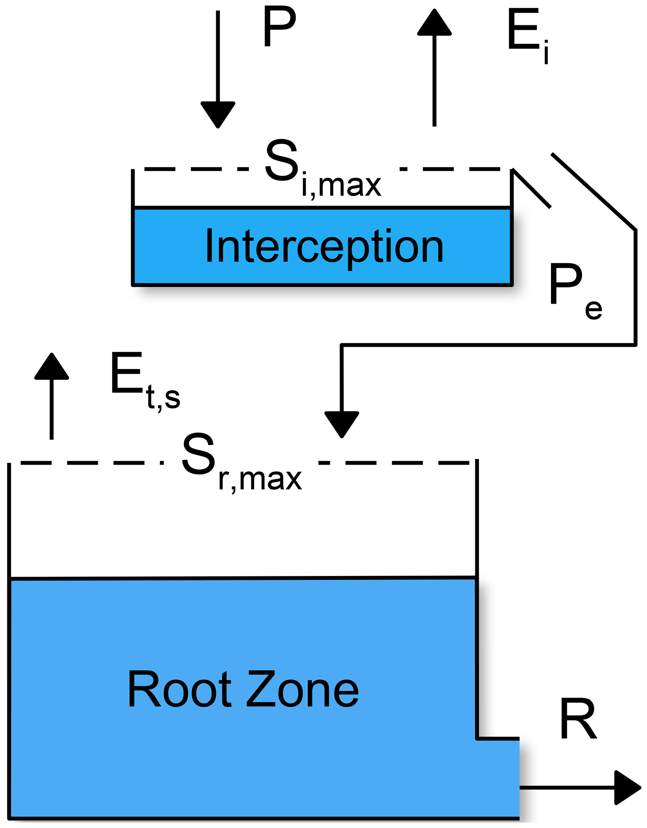
Figure 3 Conceptual model for the nonlinear recharge model. S_i, max and S_r, max are the maximum capacities of the interception and root zone reservoirs, respectively. E_i is the interception evaporation, and E_t, s is a combined flux consisting of transpiration and soil evaporation.

The general functioning of the model is as follows. Precipitation water is intercepted in the first reservoir until the interception capacity S_i,max [L] is exceeded. The intercepted water can evaporate from the first reservoir as interception evaporation (E_i [L T⁻¹]). This process forms the first barrier for precipitation to become groundwater recharge (Savenije, 2004) and creates a threshold nonlinearity in the model. Precipitation exceeding the interception capacity continues as effective precipitation (P_e [L T⁻¹]) to the root zone reservoir. From the root zone, water is evaporated through transpiration by vegetation and soil evaporation (E_t,s [L T⁻¹]) or is drained to become groundwater recharge (R [L T⁻¹]). The model is described in more detail below.

To allow the model to adjust the input potential evaporation (E_p) to an evaporation flux that better represents the vegetation-dependent actual evaporation, a maximum potential evaporation flux E_max [L T⁻¹] is computed first:

$$\begin{array}{}\text{(6)}& E_{\max }=k_{\mathrm{v}}{E}_p,\end{array}$$

where k_v [–] is a vegetation coefficient that needs to be calibrated. This approach is similar to, for example, the ecohydrological streamflow model developed by Viola et al. (2014). The parameter k_v is interpreted as a vegetation coefficient, highlighting the idea that the groundwater recharge may be affected by different types of vegetation instead of a single type of crop.

The water balance for the interception reservoir is

$$\begin{array}{}\text{(7)}& {\displaystyle \frac{\mathrm{\Delta }{S}_{\mathrm{i}}}{\mathrm{\Delta }t}}=P-E_{\mathrm{i}}-P_{\mathrm{e}},\end{array}$$

where

$$\begin{array}{}\text{(8)}& E_{\mathrm{i}}\mathrm{\Delta }t=\text{min}(E_{\max }\mathrm{\Delta }t,S_{\mathrm{i}}),\end{array}$$

where S_i [L] is the amount of water stored in the interception reservoir. The maximum storage capacity of the interception reservoir is determined by the parameter S_i, max [L]. Intercepted water is evaporated from the interception reservoir, limited by the amount of maximum potential evaporation E_max (energy-limited) or the amount of water available for evaporation S_i (water-limited). Any precipitation water exceeding the interception capacity S_i, max will continue to the root zone reservoir as effective precipitation P_e.

The water balance for the root zone reservoir is

$$\begin{array}{}\text{(9)}& {\displaystyle \frac{\text{d}{S}_{\mathrm{r}}}{\text{d}t}}=P_{\mathrm{e}}-E_{\mathrm{t},\mathrm{s}}-R,\end{array}$$

where S_r [L] is the amount of water in the root zone reservoir, E_t, s [L T⁻¹] is a combined evaporation flux constituting both soil evaporation and transpiration by vegetation, and R is the recharge to the groundwater. The maximum storage capacity of the root zone reservoir is determined by the parameter S_r, max [L]. The saturation at t=0 is set to $S_{\mathrm{r}}(t=\mathrm{0})=\mathrm{0.5}{S}_{\mathrm{r},\max }$. The evaporation flux E_t, s is limited by the amount of water available in the root zone as follows:

$$\begin{array}{}\text{(10)}& E_{\mathrm{t},\mathrm{s}}=(E_{\max }-E_{\mathrm{i}})min(\mathrm{1},{\displaystyle \frac{S_{\mathrm{r}}}{l_{\mathrm{p}}{S}_{\mathrm{r},\max }}}),\end{array}$$

where the parameter l_p [–] determines at what fraction of S_r, max the evaporation flux is limited by the availability of soil water. The relationship between the saturation of the root zone ($S_{\mathrm{r}}/S_{\mathrm{r},\max }$) and the fraction of the potential evaporation that is evaporated through the root zone ($E_{\mathrm{t},\mathrm{s}}/E_{\max }$) is shown in Fig. 4a. It is noted that the maximum potential evaporation is decreased by the amount of evaporation that already took place as interception evaporation. The actual evaporation as simulated by the nonlinear model is calculated as $E_{\mathrm{a}}=E_{\mathrm{t},\mathrm{s}}+E_{\mathrm{i}}$.

Recharge to the groundwater R is computed using Campbell's approximation for unsaturated hydraulic conductivity (Campbell, 1974).

$$\begin{array}{}\text{(11)}& R=k_{\mathrm{s}}{\left({\displaystyle \frac{S_{\mathrm{r}}}{S_{\mathrm{r},\max }}}\right)}^{\mathit{\gamma }},\end{array}$$

where k_s [L T⁻¹] is the saturated hydraulic conductivity, and γ [–] is a parameter that determines how nonlinear this flux is with respect to the saturation of the unsaturated zone. Equation (11) reduces to the equation used in the FLEX models (Eq. 4 in  Fenicia et al., 2006) when γ=1 and is similar to that used by Peterson and Western (2014). The relationship between the saturation of the root zone and the recharge flux for different values of γ is shown in Fig. 4b.

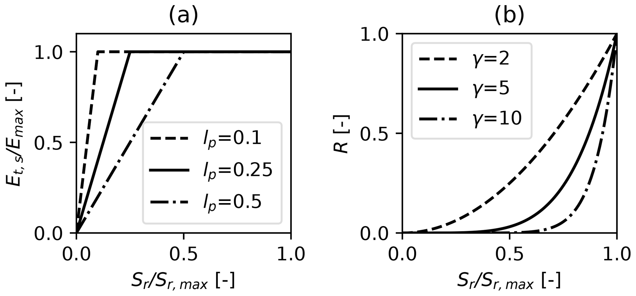
Figure 4 Relationships between the saturation of the root zone ($S_{\mathrm{r}}/S_{\mathrm{r},\max }$) and the fraction of the potential evaporation that is evaporated through the root zone ($E_{\mathrm{t},\mathrm{s}}/E_{\max }$) (a), and the drainage (R) from the root zone reservoir (b). The saturated hydraulic conductivity is set to k_s=1 mm d⁻¹.

In the preliminary phase of this study, it was found that the use of an exponential response function yields similar results to the four-parameter response function for the nonlinear model. For reasons of model parsimony, the exponential response function (Eq. 4) was adopted for the nonlinear model to translate the recharge R into groundwater levels.

In total, the nonlinear recharge model has six parameters that need to be estimated: k_v, S_i, max, S_r, max, k_s, γ, and l_p. Some of these parameters may be fixed to sensible values based on experience and literature values (Savenije, 2010), decreasing the number of parameters that need to be calibrated. Here, the interception capacity S_i, max was set to 2 mm, and l_p was fixed to 0.25 [–]. The parameter S_r, max was fixed to 250 mm (e.g., Gao et al., 2014), as it was found to have a strong correlation with k_s in the preliminary phase of this study and thus hard to calibrate. This leaves a total of six parameters to be calibrated: k_v, k_s, and γ of the nonlinear recharge model, A and a of the response function (Eq. 4), and the base level of the model d (Eq. 1).

3.4 The Lysimeter model

For comparison, a third model is constructed where the recharge measured with the lysimeters is used as the flux R in Eq. (2). Similar to the nonlinear model, an exponential response function is used to translate this recharge into groundwater levels. Assuming that the recharge measured with the lysimeters is a good estimate of the (unknown) real recharge, the groundwater levels simulated with this model provide an indication of the fit that may potentially be obtained with the other models.

3.5 Noise modeling

The residuals r(t) of TFN models applied to groundwater-level data (see Eq. 1) often show considerable autocorrelation. To allow for statistical inferences with the model (e.g., the estimation of confidence intervals of the simulated recharge), it is necessary to transform the residuals series into a noise series that is approximately white noise. For groundwater levels time series, this generally means that the autocorrelation needs to be removed from the residuals. An autoregressive model of order 1 (AR(1)) is commonly used for this purpose (e.g., von Asmuth et al., 2002):

$$\begin{array}{}\text{(12)}& \mathit{\upsilon }\left(t_i\right)=r\left(t_i\right)-r\left(t_{i-\mathrm{1}}\right){\text{e}}^{-\mathrm{\Delta }{t}_i/\mathit{\alpha }},\end{array}$$

where υ is called the noise series here, Δt_i is the time step between two residuals r(t_i) and r(t_i−1), and α [T] is the AR parameter.

In the preliminary phase of this study, the models were calibrated using daily groundwater-level observations. It was found that the noise series from these models still exhibited significant autocorrelation, despite the use of the AR(1) noise model. This result may in fact not be that surprising, considering the slow processes governing groundwater flow systems and the model structure used to simulate these. The former can for example be quantified by calculating the autocorrelations of the observed groundwater levels, which in this study are higher than 0.95 for measurements up to 13 d apart and only drop below 0.5 for measurements 100 d apart. The latter is more general, where autocorrelated errors are a result from the model structure. Errors in the input data propagate through the TFN model and are likely to result in autocorrelated errors, due to the use of a reservoir model (Kavetski et al., 2003) and the convolution with an impulse response function.

As a practical solution, the time step between groundwater-level observations was systematically increased through removal of observations from the time series. For each increase in the interval between two measurements, the models were recalibrated and diagnosed for autocorrelation using the Durbin–Watson (DW) test (Durbin and Watson, 1950) for the first time lag and the Ljung–Box test (Ljung and Box, 1978) for lags of up to 1 year. The results for the DW test for different time intervals are shown in Fig. 5a. A value of DW = 2 indicates that there is no autocorrelation in the noise, while DW < 2 indicates a positive autocorrelation at lag one and DW > 2 a negative autocorrelation. While it is clearly visible in Fig. 5a that removing observations from the groundwater-level time series reduces the autocorrelation, application of the AR(1) model did not suffice for the data used in this study.

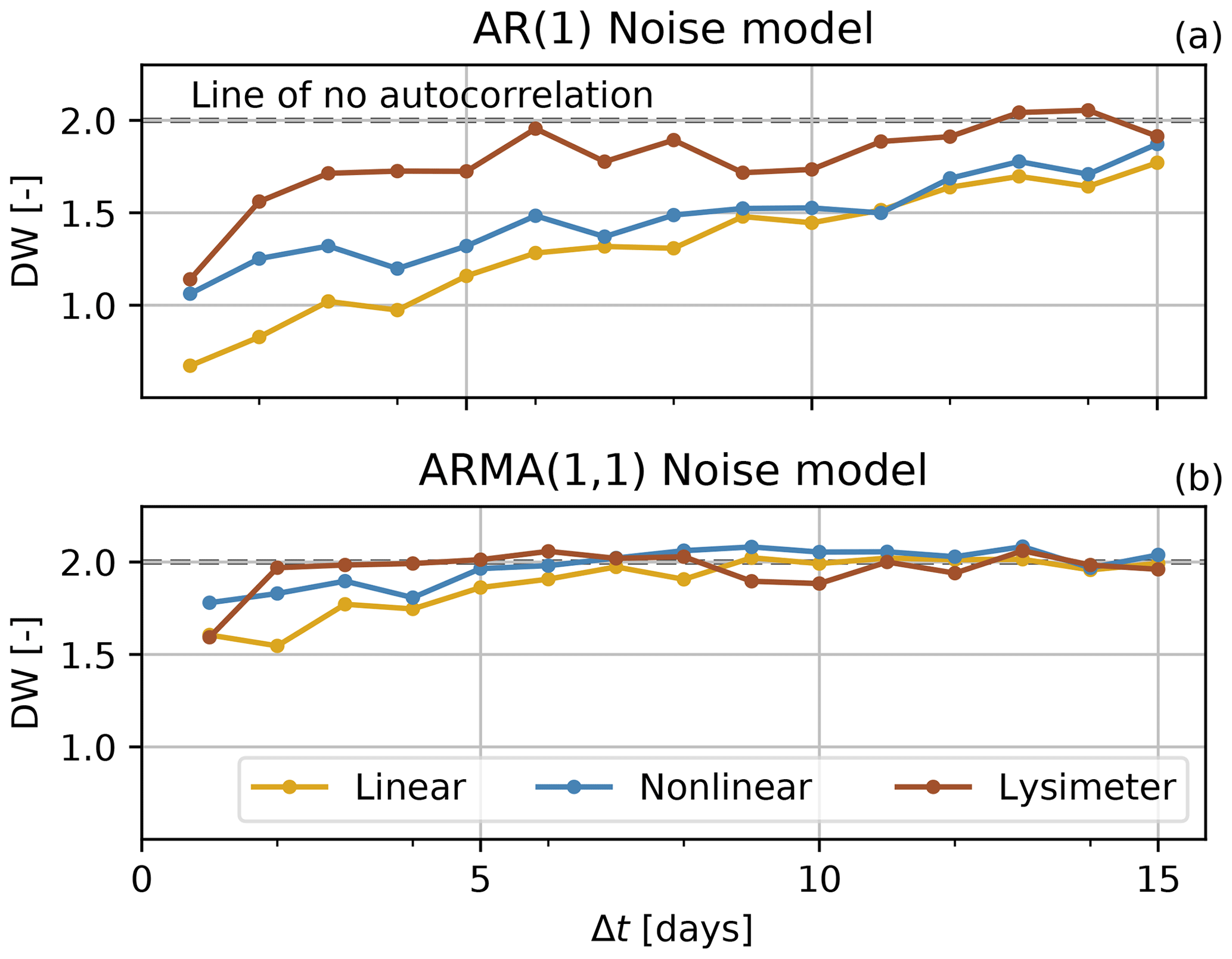
Figure 5 Durbin–Watson (DW) statistics for models calibrated on groundwater levels with an increasing interval (Δt) up to 15 d, using an AR(1) noise model (a) or an ARMA(1,1) noise model (b).

In a further attempt to remove the autocorrelation from the residuals, the AR(1) model was extended with a moving-average part of order 1 (MA(1)) to form an ARMA(1,1) noise model as follows:

$$\begin{array}{}\text{(13)}& \begin{array}{rl}& \mathit{\upsilon }\left(t_i\right)=\\ & r\left(t_i\right)-r\left(t_{i-\mathrm{1}}\right){\text{e}}^{-\mathrm{\Delta }{t}_i/\mathit{\alpha }}-{\displaystyle \frac{\mathit{\beta }}{\left|\mathit{\beta }\right|}}\mathit{\upsilon }\left(t_{i-\mathrm{1}}\right){\text{e}}^{-\mathrm{\Delta }{t}_i/\left|\mathit{\beta }\right|}i\ge \mathrm{1}\end{array},\end{array}$$

where β is the parameter of the moving-average part of the noise model. The parameter β can have both positive and negative values in this formulation. The parameters α and β are estimated during model calibration. The first value of the noise series at t=0 is set to the first value of the residuals, υ(t₀)=r(t₀)), as it is not possible to compute υ(t=0) from the previous residual. The MA(1) process can correct for individual shocks in the system, quickly reducing the error over one time step, whereas the AR(1) part deals with an error whose effect exponentially decreases over multiple time steps. Note that the time step Δt in Eq. (13) may be irregular, but in this study only time series with a regular time step are used. Additional research is necessary to make this noise model fully applicable to irregular time steps, as was done for the AR(1) model (von Asmuth and Bierkens, 2005).

Rerunning the previous analysis of the Durbin–Watson statistic for an increasing time interval between observations using the ARMA(1,1) noise model shows that this noise model is more capable of removing the autocorrelation at the first time lag (Fig. 5b). The autocorrelation decreases with increasing time interval, and the DW value stabilizes for time intervals of around 6 d and larger. A lack of autocorrelation in the noise series at larger time lags was also confirmed using the Ljung–Box test, although the autocorrelation at lags of around 1 year become significant for time intervals below 10 d. Based on this analysis, groundwater-level time series with a 10 d time interval were used for model calibration. The final autocorrelation plots are shown in Fig. A1 in the Appendix.

Figure 6 Modeling strategy as applied in this study.

3.6 Parameter estimation and confidence intervals

The previous three sections described the TFN models used in this study, which include a recharge model, a response function, and an ARMA(1,1) noise model. An overview of the entire TFN modeling process is shown in Fig. 6. The model parameters are estimated by fitting the simulated groundwater levels to the observed groundwater levels. The linear and nonlinear models both have eight parameters that are estimated, and the lysimeter model has five parameters. A nonlinear least-squares approach is used here to estimate the parameters for each model simultaneously. The following objective function is used, minimizing the sum of the squared noise:

$$\begin{array}{}\text{(14)}& F_{\mathrm{obj}}=\sum _{i=\mathrm{1}}^n{\mathit{\upsilon }}_i^{\mathrm{2}}.\end{array}$$

Minimization of the objective function is done using the trust-region-reflective algorithm, as implemented in SciPy's least-squares method (Virtanen et al., 2020, version 1.4.0) and Lmfit (Newville et al., 2019, version 1.0). Note that this is not the default option in Lmfit. The standard errors of the parameters are computed from the covariance matrix that is estimated during optimization. An important assumption underlying this approach is that the minimized noise series (υ in Eq. 13) behaves as normally distributed white noise with no significant autocorrelation, a constant variance (homoscedastic), and a mean of zero. These assumptions were checked through visual inspection of the results and the use of various statistical tests for autocorrelation as already shown in the previous section.

The 95% confidence intervals of the simulated recharge are computed through a Monte Carlo simulation (N=100 000). Parameter sets are drawn from a multivariate normal distribution computed using the estimated covariance matrix. If one of the parameters in a parameter set is outside the parameter boundaries, the set is discarded from the sample, and a new parameter set is drawn. This procedure is repeated until N parameter sets are available for the Monte Carlo simulation. The model is run with the N different parameters sets, and the 95 % confidence intervals are computed from the ensemble of simulated recharge fluxes.

3.7 Numerical and software implementation

All models were implemented in Python code and are freely available through the open-source package Pastas (Collenteur et al., 2019, version 0.17). The nonlinear model is available under the name “FlexModel” in the Pastas library. The nonlinear recharge model is numerically solved using an explicit Euler scheme with a time step of 1 d. As TFN models are traditionally computationally inexpensive and have short computation times (in the order of seconds), special attention was paid to increase the computation speed of the recharge model. This was achieved by using Numba, a just-in-time compiler for Python code (Lam et al., 2015, version 0.49). As a result, the nonlinear model has similar computation times to the linear model.

3.8 Goodness-of-fit metrics

Four metrics are used to evaluate the goodness-of-fit of the simulated groundwater levels and the groundwater recharge: the mean absolute error (MAE), the root mean squared error (RMSE), the Nash–Sutcliffe efficiency (NSE), and the Kling–Gupta efficiency (KGE). The MAE and the RMSE provide a metric for the overall model fit and error, while the NSE is a goodness-of-fit metric commonly used in hydrological modeling. The KGE is an aggregate metric and contains a correlation term, a bias term, and a variability term (see Kling et al., 2012, for a more detailed discussion). The NSE and KGE all have a maximum of 1, denoting a perfect fit of the model with the data. The MAE and RMSE improve when moving towards zero.

4 Results

4.1 Groundwater-level simulations

The 10-year period 2007–2016 was used for calibration, and the 3-year period 2017–2019 was used for model validation. The year 2006 was used for model warm-up. The use of a warm-up period is especially important for the nonlinear model because the recharge flux strongly depends on the initial saturation level of the root zone. The simulated and the observed groundwater levels are shown in Fig. 7a, along with the estimated recharge fluxes (Fig. 7b and c) and the measured recharge (Fig. 7d). As the models are calibrated on groundwater-level observations with a 10 d time step, only recharge rates summed over 10 d intervals are presented here. The values of the calibrated parameters can be found in Table A1 in the Appendix.

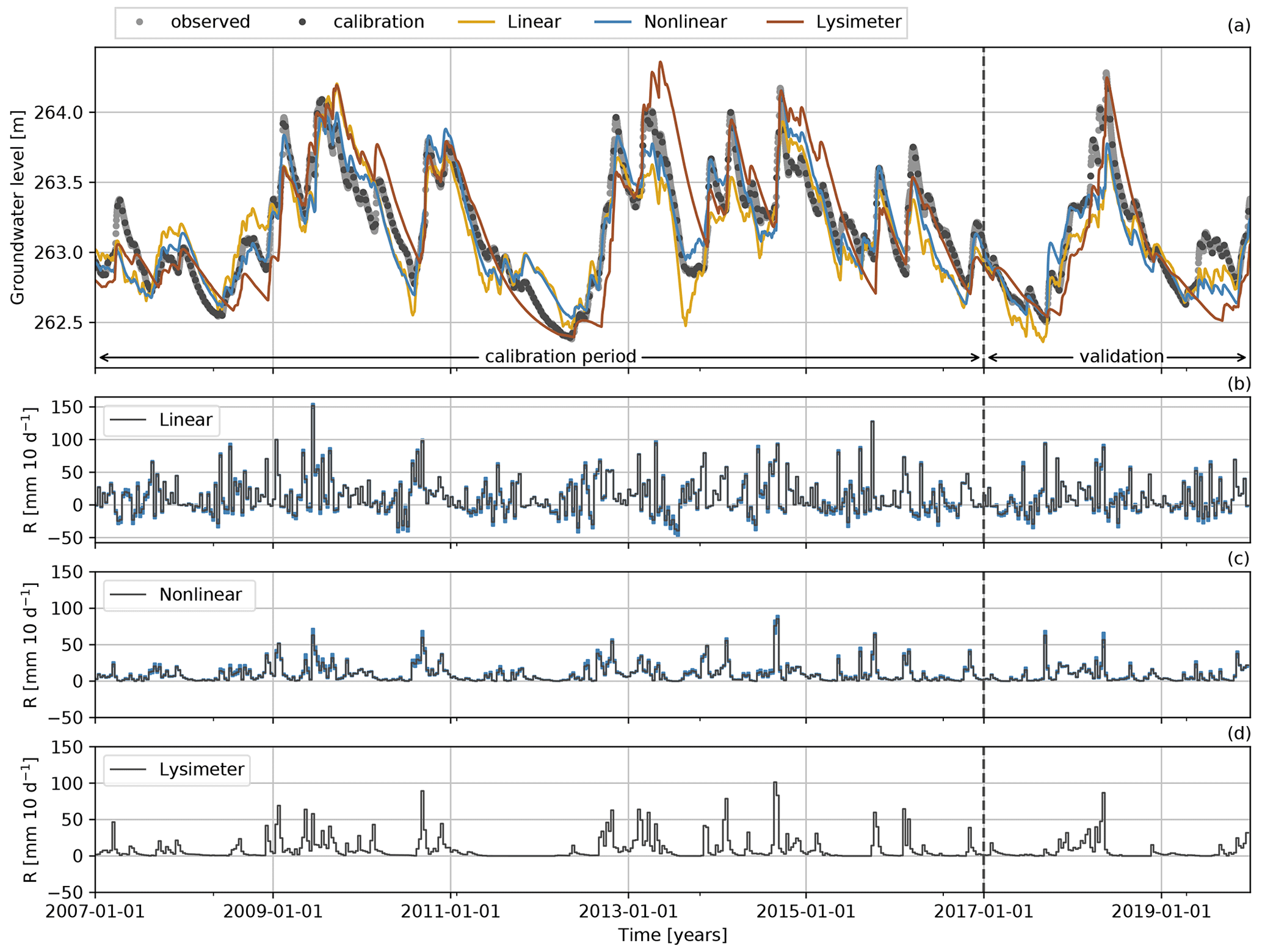
Figure 7 Observed and simulated groundwater levels (a) and the estimated (b, c) and measured (d) recharge rates (R). The groundwater-level measurements used for calibration are shown as black dots, and unused measurements are shown as gray dots. The blue shading in plots (b) and (c) denotes the 95 % confidence intervals of the recharge estimates.

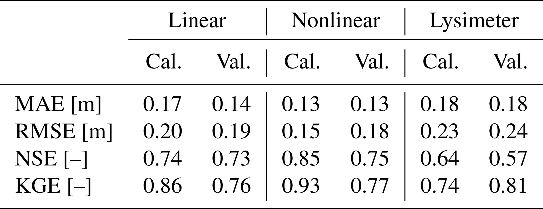
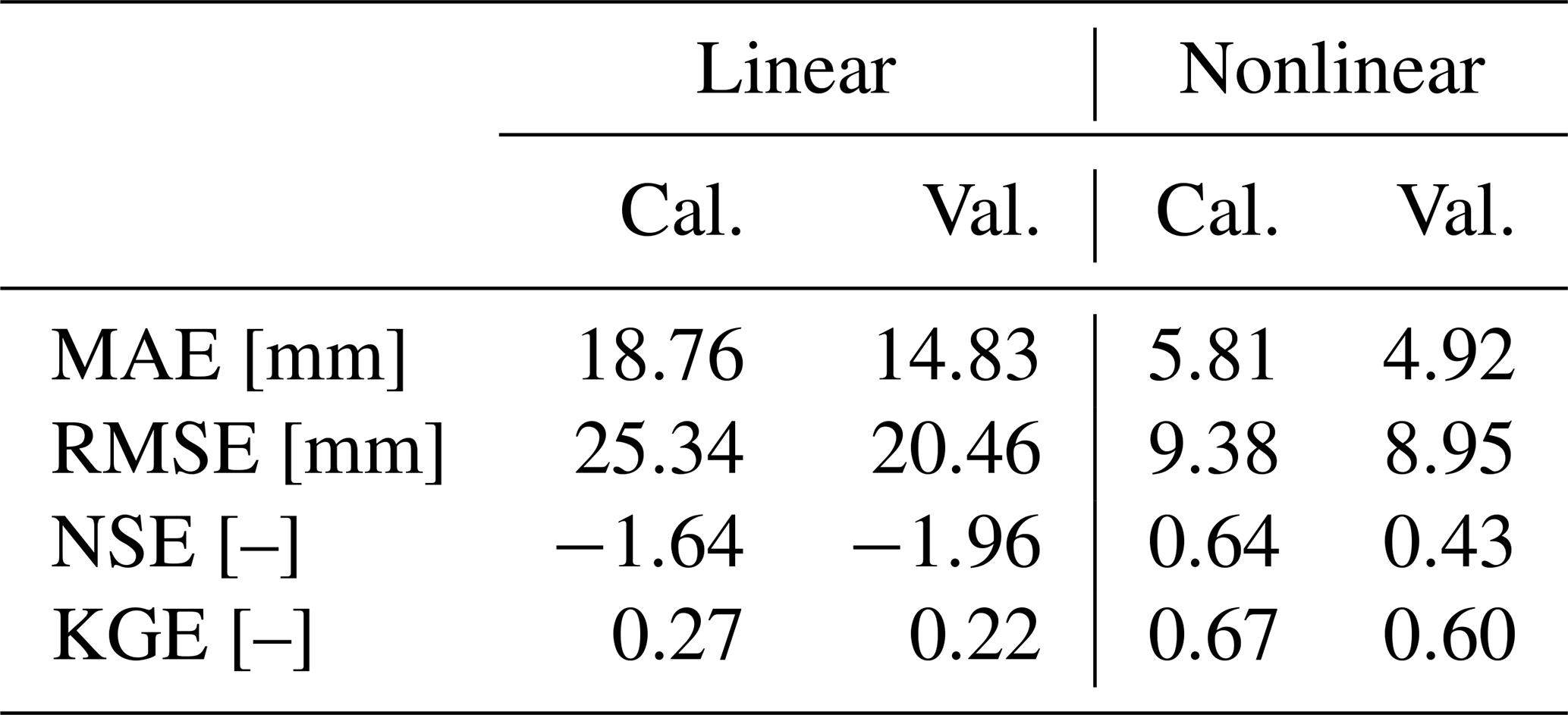
All three TFN models are able to capture the major groundwater dynamics and simulate the observed groundwater levels reasonably well. For the calibration period, the nonlinear model shows the best simulation of the groundwater levels as quantified by the four goodness-of-fit metrics used in this study (see Table 1). The linear model performs better than the lysimeter model according to all four metrics. For the validation period, the differences in the metrics are not as clear, but the nonlinear model still outperforms the other models. The lysimeter model captures the single peak in groundwater levels during the validation period better than the other models but shows the worst simulation of the low groundwater levels that follow this peak. The linear model performs better during the period with low groundwater levels but overestimates the low groundwater levels observed at the beginning of the validation period. The nonlinear model generally shows good performance but underestimates the low groundwater levels at the end of the validation period.

Table 1 Goodness-of-fit metrics for the groundwater-level simulation for each model. The metrics are computed for the calibration period (2007–2016) and the validation period (2017–2019). Groundwater-level measurements with a 10 d time interval were used to calculate these metrics, similar to the measurements used for calibration.

While the groundwater levels simulated by the linear and nonlinear models are rather similar, the groundwater recharge fluxes (R) computed by these two models are very different (see Fig. 7b and c). The recharge fluxes are compared to the recharge measured with the lysimeters by computing the same goodness-of-fit metrics (Table 2). The recharge flux computed by the nonlinear model shows a reasonably good fit resulting in, for example, a Kling–Gupta efficiency of KGE = 0.67 for the calibration period. The recharge computed by the linear model, however, deviates strongly from the lysimeter recharge and often simulates negative recharge that was not measured with the lysimeters. It is concluded that the linear model should not be used to estimate groundwater recharge at this small timescale (10 d intervals), as expected. For the simulation of groundwater levels, the linear model may still be appropriate, as the difference in the recharge flux can be compensated for by the shape of the response function. This is clearly the case here, as is visible by the differences in the block and step response functions calibrated for each model (shown in Fig. 8). The linear model shows a delayed response to a groundwater recharge impulse, whereas the nonlinear and lysimeter models simulate an instantaneous response of the groundwater levels.

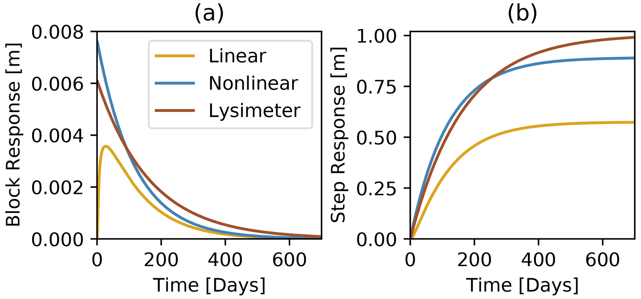
Figure 8 Calibrated block and step response functions for all three models. The block response (a) shows how the groundwater levels react to a 1 d recharge event of 1 mm. The step response (b) shows the response of the groundwater level to a sudden unit increase in recharge that extends infinitely in time.

Although the linear recharge model in combination with the four-parameter response function works well to simulate most of the groundwater levels time series, the model fails under conditions where evaporation is limited by the availability of soil moisture. This occurs for example in the years 2010, 2013, and 2017, when the linear model simulates a stronger decline in groundwater levels than was observed. These strong declines in simulated groundwater levels are caused by continued (modeled) evaporation over the summer months, resulting in negative recharge rates (as visible in Fig. 7b) and ultimately lower groundwater levels. Measurements from the lysimeters (data not shown) show that actual evaporation is only a fraction of the potential evaporation during those periods. Similar behavior for the simulation of low groundwater levels was found by Berendrecht et al. (2006), using the same linear recharge model. These results confirm that the linear recharge model should not be used to simulate groundwater levels under such soil-moisture-limited conditions.

Table 2 Performance metrics for the similarity between the estimated recharge and the measured recharge, in millimeters per 10 d. The metrics are shown for the calibration period (2007–2016) and the validation period (2017–2019).

The nonlinear model performs much better under such soil-moisture-limited conditions and simulates almost no recharge during these periods. The nonlinear model resembles the recharge behavior as measured with the lysimeters reasonably well, recharge occurring primarily as individual events, interspersed with extended periods of reduced recharge. The behavior of event-based recharge was also found in other studies (Groenendijk et al., 2014; Reszler and Fank, 2016) and suggests that recharge paths are activated when a certain threshold in the soil moisture is exceeded. This nonlinear response of recharge to infiltrating precipitation also becomes clear when examining the estimated values for the parameter γ, which indicates a nonlinear response with a value of γ=2.91 [–]. The results show that the use of a nonlinear recharge model improves the simulation of groundwater levels at the study site while also providing a reasonable estimate of the recharge flux R at this timescale.

It is somewhat surprising that the lysimeter model does not outperform the other two models. Three periods with deviating groundwater levels that stand out in particular are discussed here: the low groundwater levels in 2011, the peak in 2013, and a low in 2015. As the groundwater-level fluctuations are primarily the result of individual recharge events, and the groundwater system has a long memory, such periods with groundwater levels deviating for a longer period of time are likely the result of errors in the quantification of individual recharge events. In 2011, almost no recharge was recorded in the lysimeters, coinciding with an underestimation of the simulated groundwater levels. From the groundwater-level measurements, however, it is clear that some recharge must have taken place, visible by temporarily stagnating and even slightly increasing groundwater levels during that period. Due to a technical issue with the lysimeters, no groundwater recharge was recorded by the lysimeters for parts of 2015, explaining the deviation in simulated groundwater levels in that year. No explanation could be found for the peak in 2013, but this may just as well be an error in the measurement of a single event, causing a long-term deviation in the groundwater-level simulation.

4.2 Annual recharge rates

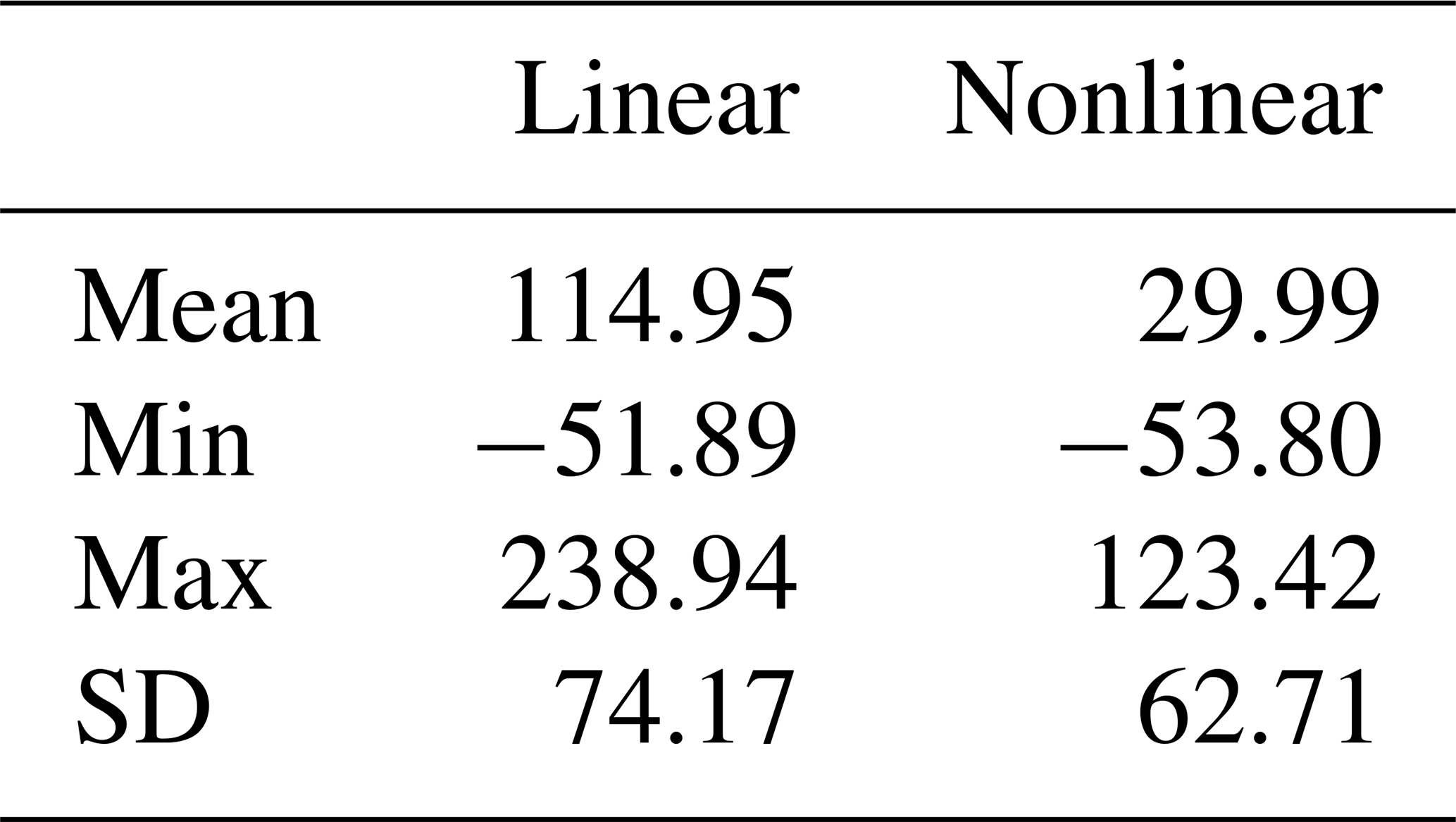
Groundwater resource managers are often interested in annual recharge rates. In this section the ability of the models to estimate recharge at this timescale is investigated. The annual recharge rates computed by the TFN models and the annual recharge measured with the lysimeters are shown in Fig. 9. The nonlinear model performs better than the linear model, also shown by the descriptive statistics of the deviation [mm] between measured and estimated annual groundwater recharge rates shown in Table 3. This is particularly true for wet years, for which the linear model shows large deviations (up to 239 mm yr⁻¹) in the annual recharge rates. The largest deviation for the nonlinear model occurs during the dry year of 2011 (123 mm yr⁻¹). The recharge computed with the linear model has much wider confidence intervals, despite (or maybe because of) having only one calibration parameter (f in Eq. 5). This means that the practical use of the recharge estimate from the linear model may be limited, as any analysis that uses this estimate as input data would have large uncertainties in its outcomes due to the uncertainty in the input data. The nonlinear model performs much better in this respect.

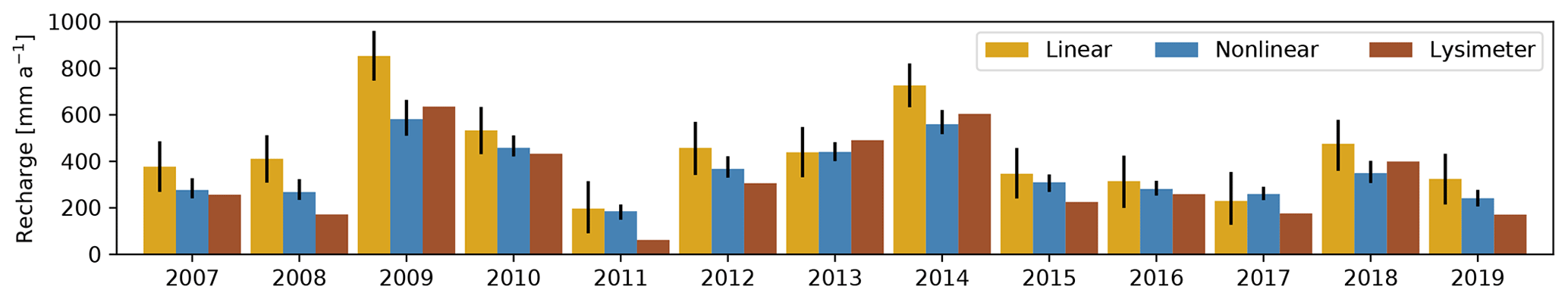
Figure 9 Annual recharge rates as computed by each TFN model and as measured with the lysimeters. The error bars denote the 95 % confidence intervals of the recharge estimate.

Table 3 Descriptive statistics of the deviation (in mm) between measured and estimated annual groundwater recharge rates.

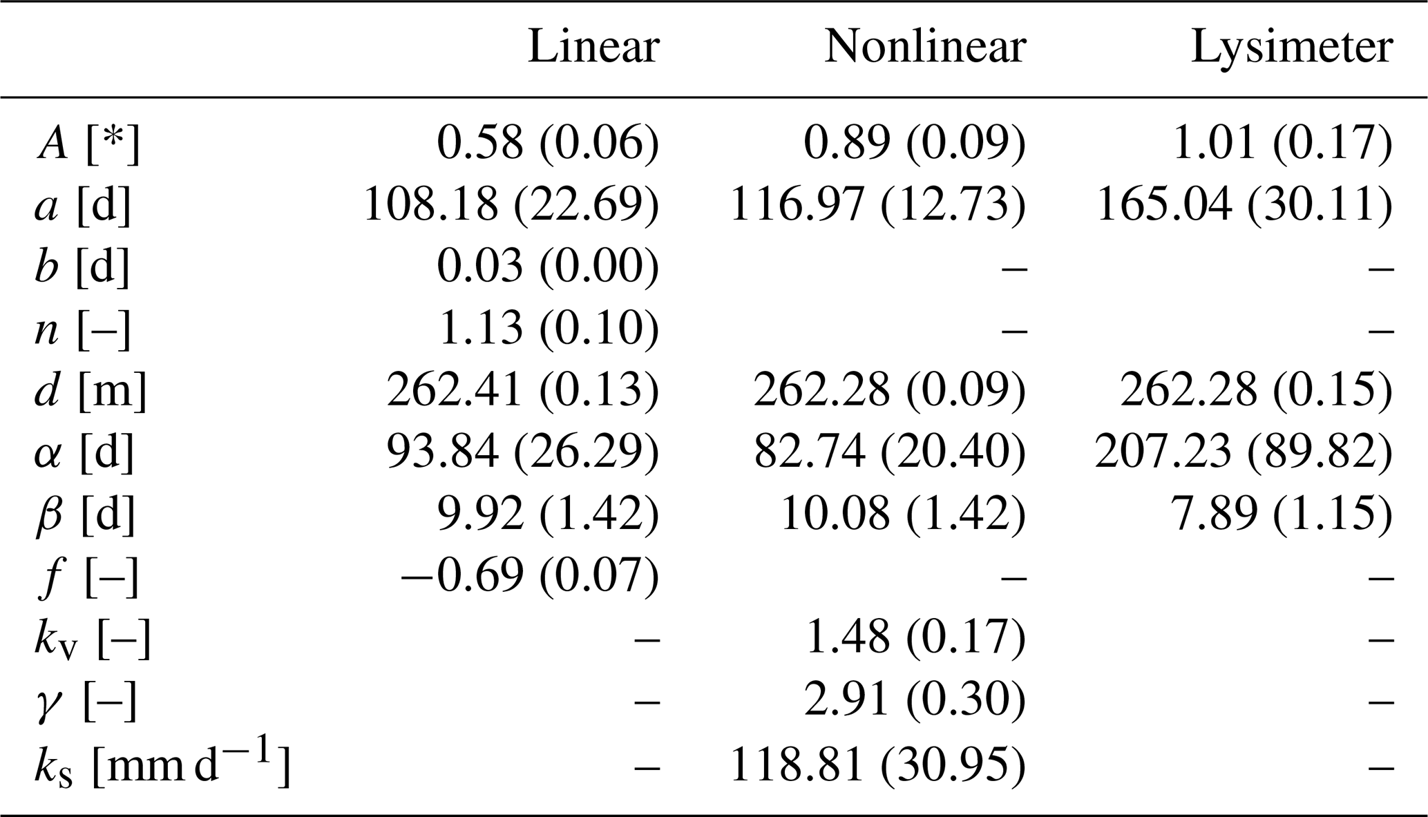
The long-term average recharge (calculated for the period 2007–2019) estimated by the nonlinear model (352 mm d⁻¹) is much closer to the recharge measured with the lysimeters (322 mm d⁻¹) than to that of the linear model (437 mm d⁻¹). The overestimation of recharge by the linear model can be explained by an underestimation of evaporation that results from a low value for the evaporation factor f in Eq. (5), $f=-\mathrm{0.69}$. From the actual evaporation flux computed from the lysimeter data (Klammler and Fank, 2014), however, it was calculated that the actual evaporation is approximately 88 % of the potential evaporation (or, f=0.88) for the period 2007–2019. These results confirm findings from Obergfell et al. (2019) that the factor f is difficult to estimate and hampers the accurate estimation of recharge using the linear model.

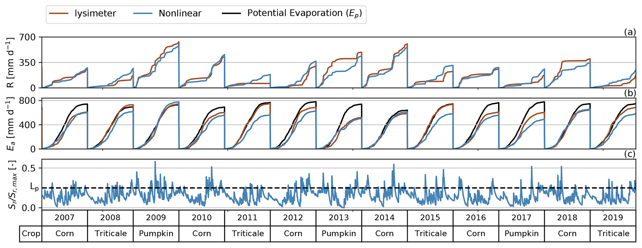
Figure 10 Yearly cumulative sums of recharge (a), the actual and potential evaporation (b), and the saturation of the root zone (c). The dashed line in plot (c) denotes the value of l_p, where the evaporation from the root zone will equal the potential evaporation.

An accurate estimate of evaporation is also important for recharge estimates made with the nonlinear model. In Fig. 10 the annual cumulative sums of recharge and actual evaporation are shown as simulated by the nonlinear model and measured with the lysimeters (computed from 1 January to 31 December). The actual evaporation computed by the model is close to that measured with the lysimeters, averaging 81 % of the potential evaporation. The vegetation coefficient k_v in Eq. (6) is calibrated at k_v=1.48 [–], which seems quite high at first. For most of the simulation period, however, the saturation of the root zone ($S_{\mathrm{r}}/S_{\mathrm{r},\max }$) is well below the level (l_p=0.25) where evaporation from the root zone equals the potential evaporation that is left after interception evaporation, as visible in Fig. 10c. As a result, the actual evaporation simulated by the nonlinear model is still below the potential evaporation but matches the actual evaporation measured with the lysimeters rather well.

In Fig. 10 it is visible that for years where the actual evaporation computed by the nonlinear model more or less equals the actual evaporation measured with the lysimeter, the recharge fluxes match better as well. When actual evaporation is underestimated by the model, the recharge is overestimated (see, e.g., 2008, 2011, and 2015), relative to the lysimeter recharge. A probable cause for the underestimation of evaporation is the cultivation of different crops in the lysimeters during the observation period (shown in the table below the plots in Fig. 10). For example, for all years when triticale was planted, the actual evaporation was underestimated and the recharge overestimated. As grass reference evaporation was used as input data, and the vegetation coefficient k_v is assumed to be constant through time, the different evaporative capacities of the individual crops is not considered in the current model setup. Cultivation of different crops does not only influence the total yearly evaporation, but also the pattern in time as a result of different growing seasons and harvest times. Such effects can again be observed for triticale, a crop that starts transpiring early in the year, visible by an earlier rise of the cumulative evaporation in years when triticale is planted. The use of improved input data for evaporation, taking into account the impact of vegetation on this flux, may further improve recharge estimations and groundwater-level simulations, particularly in agricultural areas with crop rotation schemes.

4.3 Parameter estimation and consistency of model output

The results presented so far are based on the calibration of the models using only 1 out of every 10 groundwater-level measurements. The use of only a selection of the available groundwater-level measurements during calibration allowed for a further investigation into the consistency of the modeling results, by calibrating the models to 10 different selections derived of the original time series as a type of split-sample test. This way, it is possible to assess the consistency of the estimated parameters and the impact on the simulated groundwater levels and the annual recharge estimates for this particular time series. The resulting ensembles of groundwater-level simulations and annual groundwater recharge estimates are shown in Fig. A2 in the Appendix. The results show that both the simulated groundwater levels and the estimated recharge fluxes are consistent between the different calibrations for all models. This should in fact not be that surprising, considering that the time series used for calibration originate from the same groundwater-level time series.

What may be more surprising, however, are the differences in the estimated parameters between the 10 different calibrations (see Fig. A3 in the Appendix). The parameter values for all models are of the same order of magnitude, and model performance measured as NSE is relatively stable, but the optimal parameter values can differ significantly from each other between calibrations (e.g., for the nonlinear model k_s ranges between 100 and 250 mm d⁻¹), even though the estimated confidence intervals overlap for the most part. The results of this split-sample test raise the question of parameter identifiability. Given the similarity in simulated groundwater levels and annual recharge estimates, it is clear that different combinations of parameters yield similar results. It is noted here that this analysis does not constitute a formal sensitivity analysis of the parameters, for example, by varying one parameter and analyzing the changes in the estimated recharge or simulated groundwater levels. The results of this split-sample test rather serve as a motivation for such a study and show that caution is needed when interpreting values of individual (optimal) parameters. Further research is necessary on the identification of parameters, for example through testing the models on large samples of groundwater time series (similar to, e.g., Perrin et al., 2001).

5 Discussion

5.1 Choice and performance of nonlinear recharge models

The results from this study showed that, compared to the linear model, the nonlinear recharge model is more capable of simulating true system dynamics that are commonly not measured, such as groundwater recharge and actual evaporation. This suggests that the improvements in the simulation of the groundwater levels and the estimation of recharge are the result of a better representation of the hydrological processes, rather than the result of added mathematical complexity. As such, the use of nonlinear recharge models in TFN models is a promising step in the effort “to get the right answers for the right reasons”, as advocated by, e.g., Kirchner (2006). This may be particularly important when using this type of models to forecast groundwater recharge and levels under drought conditions.

It is noted that the nonlinear recharge model developed for this study is only one of a set of similar soil-water storage models that may be applied. Comparable results (not shown here) were obtained using the nonlinear recharge model developed by Berendrecht et al. (2006), which is also available in the Pastas software (Collenteur et al., 2019). It is expected that other nonlinear models (e.g., the models of Peterson and Western, 2014) perform similarly. The identification of the most appropriate nonlinear recharge model under different conditions is a topic for future investigation.

The application of a nonlinear recharge model does come with additional challenges in the estimation of the model parameters. Nonlinear models have a larger number of parameters that need to be estimated and a higher potential for problems related to equifinality (Beven, 2006). As was shown in this study, however, not all model parameters have to be calibrated, and some may be fixed to sensible values (following e.g., Savenije, 2010). The use of nonlinear models therefore does not necessarily imply a higher number of parameters that need to be calibrated; i.e., the same number of parameters were calibrated for the linear and nonlinear models used in this study. Nonetheless, finding the optimal parameter values may be challenging and dependent on the initial parameter values. Global optimization methods may help overcome these problems, as for example shown by Peterson and Western (2014).

5.2 Transformation of the residuals to uncorrelated noise

In this study, model parameters were estimated by fitting simulated groundwater levels to observed groundwater levels. The recharge is an intermediate model result that is not calibrated for. It is recommended here to quantify the impact of parameter uncertainties on the recharge estimates by computing their confidence intervals using the standard errors of the estimated parameters. Reliable estimates of the standard errors of the parameters may be obtained in the current framework when the autocorrelation of the minimized noise series is removed by using an appropriate noise model. Here, an AR(1) model did not suffice for this purpose, and an ARMA(1,1) noise model was used instead. The current implementation of the ARMA(1,1) model is for groundwater-level time series with regular time steps between observations, unlike the AR(1) model that is often used (von Asmuth and Bierkens, 2005). Additional work is needed to make the ARMA(1,1) model suitable for time series with irregular time steps.

The ARMA(1,1) noise model performed reasonably well in transforming the residual series into a noise time series that is approximately white noise, but some autocorrelation remained in the noise series. As a practical solution, the time interval between groundwater-level measurements was increased to 10 d by removing measurements from the time series. It is noted here that the optimal time interval is likely to be site-specific and should be investigated for each individual time series. The approach shown in Sect. 3.5 can be helpful in determining the optimal time step size used for model calibration. Alternatively, it may be appropriate to use an ARMA model of higher order (see, e.g., Box and Jenkins, 1970). The modeling of the residuals and the choice of an appropriate noise model and time interval are an iterative process, as also suggested by Smith et al. (2015). Additionally, it is important to use an appropriate length for the calibration period. Van der Spek and Bakker (2017) recommended a 10- to 20-year period for simulating groundwater levels with reliable credible intervals.

5.3 Application to other hydrogeological settings

The presented approach was tested on relatively shallow groundwater levels (±4 m depth to the water table), for which no feedback between the groundwater and root zone was expected. In this setting, an exponential response function was used in the nonlinear model, and the computed flux R could be directly interpreted as groundwater recharge. The use of an exponential function may not be appropriate for deeper groundwater bodies with thicker unsaturated zones, which require a more complicated response function that accounts for a significant travel time through the unsaturated zone. In that case, the estimated flux R should be interpreted as drainage from the root zone to the groundwater and not as recharge occurring at the water table. Alternatively, as suggested by Peterson and Fulton (2019), the flux could be “averaged over a period greater than the time lag” between the drainage from the root zone and the arrival at the water table, to provide an estimate of gross recharge at larger timescales.

It is not always possible to assume that there is no feedback between the root zone and the groundwater. If the roots of the vegetation reach the groundwater, for example in shallow groundwater systems or deep rooting systems, evaporation of groundwater can occur. In this case, the actual evaporation is not limited by the availability of soil moisture and may be close to potential evaporation. The linear model may be applicable to simulate groundwater levels and estimate recharge in these systems, although the model still lacks the ability to temporarily store water. An alternative nonlinear modeling approach that allows for the evaporation of groundwater (Peterson and Western, 2014) may be more appropriate under these conditions. In this approach, the part of the potential evaporation that is not lost through evaporation and transpiration from the soil reservoir is added to the TFN model as a separate forcing.

Additional hydrological processes (e.g., snowmelt, surface runoff) and forcings (e.g., pumping, river levels) may be included in the model to make the methods applicable in other hydrogeological settings than those presented here. In the current framework, it is relatively easy to account for other forcings causing groundwater-level fluctuations (e.g., von Asmuth et al., 2008; Collenteur et al., 2019). This allows for the estimation of recharge in hydrogeological systems where the groundwater-level fluctuations are not exclusively the result of recharge. Obergfell et al. (2019) already successfully tested this approach to estimate recharge from groundwater levels that were also influenced by groundwater pumping. Additional processes may be implemented in the root zone model to make the recharge models applicable in different settings, for example precipitation entering the system as snow or leaving as surface runoff before infiltrating into the soil. For ideas on how to include such processes, one can draw from the vast number of concepts already available in conceptual rainfall-runoff modeling (e.g., Beven, 2011).

6 Conclusions and outlook

In this study, the application of linear and nonlinear transfer function noise (TFN) models using predefined impulse response functions was explored to estimate recharge and simulate groundwater levels. The models were calibrated to groundwater levels observed at the study site in Wagna, Austria. The recharge estimate, obtained as an intermediate flux of the models, was compared with the average seepage measured with two lysimeters at the same site. This enabled an evaluation even at short timescales, which goes beyond earlier related work. Three models were applied. In the first, recharge was calculated as a linear function of precipitation and evaporation, while the second used a nonlinear recharge model for this purpose. A third TFN model was constructed for comparison, using the lysimeter measured seepage as input data to simulate the groundwater levels.

Based on the results from this study, it is concluded that it is possible to estimate groundwater recharge from observed groundwater-level time series using TFN models and impulse response functions. This confirms findings from previous research (Obergfell et al., 2019; Hocking and Kelly, 2016; Peterson and Fulton, 2019), for a different geographic and climatic area. The nonlinear recharge model provided better estimates of annual recharge rates than the linear model and was shown to compute reasonable estimates for recharge summed over 10 d periods. This suggests that the nonlinear model may be used to obtain recharge estimates at smaller timescales than reported so far. Using detailed information from the lysimeters present at the study site, deviations in the recharge estimate could be linked to errors in the simulation of the actual evaporation, highlighting the importance of the evaporative flux in the estimation of recharge.

The use of a nonlinear recharge model also improved the simulation of the groundwater levels compared to the linear model. For the linear model, a more complex response function was required to obtain satisfactory results, as the response function also had to simulate the storage effects of the root zone. The response function used in the linear model did not compensate for all hydrological conditions. The lack of storage dynamics in the linear model leads to larger errors in the simulation of the groundwater levels during periods of droughts, when transpiration and soil evaporation are limited by soil moisture availability. These findings confirm those from other studies (Berendrecht et al., 2006; Peterson and Western, 2014) and advocate a more widespread adoption of nonlinear recharge models in TFN modeling of groundwater levels.

The proposed method for estimating recharge combines the advantages of data-driven TFN models with those of soil-water storage models. Adding the latter to the TFN model improves the representation of hydrological processes and enables recharge estimation at subseasonal timescales and below. As the model parameters are obtained by calibration to measured groundwater levels, knowledge of soil and aquifer properties is not needed. This makes the methods particularly useful for areas with little information about the subsurface. The methods developed in this paper were tested on a single groundwater time series and are presented as a proof-of-concept. Additional research is needed using larger groundwater-level data sets to investigate the general applicability of the method under different hydrogeological settings and to explore the suitability of different types of recharge models.

Appendix A

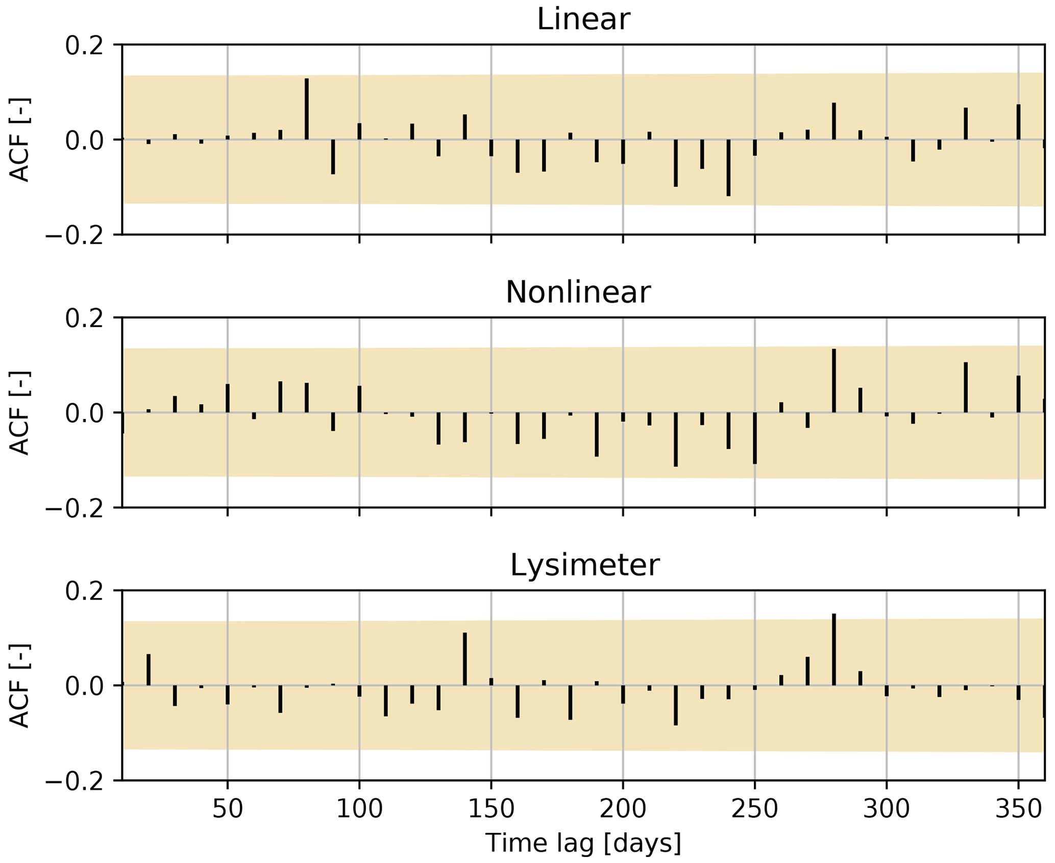
Figure A1 Autocorrelation graphs for all three models for lags of up to 1 year. The shaded area shows the 99 % confidence interval for the autocorrelation function (ACF).

Figure A2 The first three plots show ensembles of 10 groundwater levels time series simulated by the three models. The bottom plot shows the mean of the estimated annual recharge rates from an ensemble of 10 models. The black whiskers show 1.96 times the standard deviations of the ensemble of annual recharge rates.

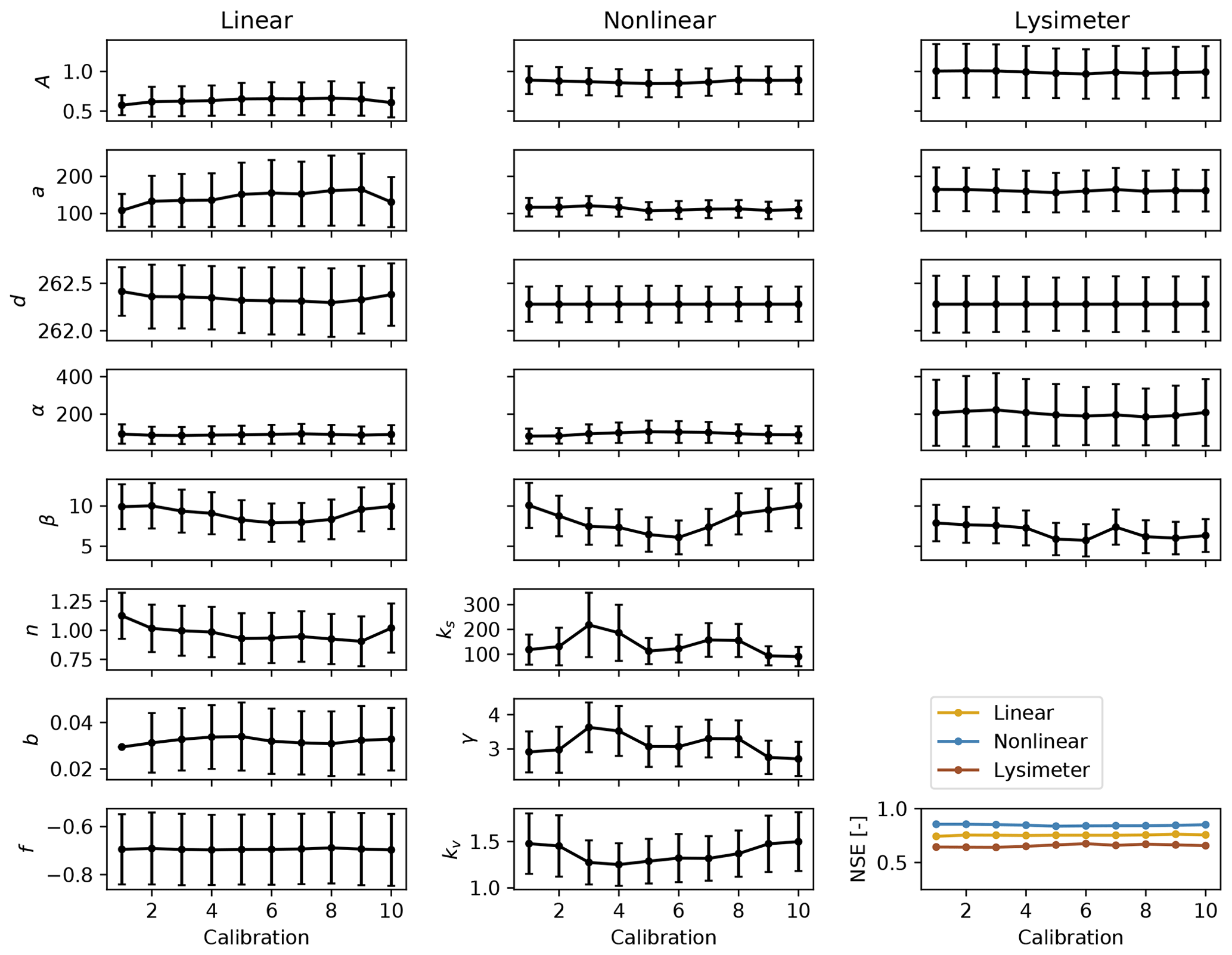
Figure A3 Parameter values and their 95 % confidence interval for the three models calibrated on 10 time series. Note that when possible, the y axis is shared between the different columns for comparison purposes. The bottom right subplot shows the model performance for each calibration, measured as the NSE between the observed and simulated groundwater levels.

Table A1 Calibrated parameter values for all three model configurations. The estimated standard errors of the parameters are reported between the brackets. The units from parameter A depend on the type of response function.