the Creative Commons Attribution 4.0 License.
the Creative Commons Attribution 4.0 License.
 | 19 Jan 2021
Modelling the hydrological interactions between a fissured granite aquifer and a valley mire in the Massif Central, France
Arnaud Duranel
Julian R. Thompson
Helene Burningham
Philippe Durepaire
Stéphane Garambois
Robert Wyns
Hervé Cubizolle
We developed a high-resolution MIKE SHE/MIKE 11 model of a 231.3 ha headwater catchment in the granitic uplands of the French Massif Central to estimate the contribution of groundwater upwelling to the water balance of the Dauges mire, an acidic valley mire of international importance for nature conservation. We estimated that groundwater upwelling from the underlying weathered granite formations – mostly an approximately 55 m deep fissured zone – provides 27.1 % of total long-term inflows to the mire. This contribution increases to 37.2 % in September when total inflows are small. Overland boundary inflow accounts for an average of 40.2 % of total inflows. However, most of this originates from groundwater seepage through mineral soils along the mire margins or in small non-channelised valleys upslope of the mire. A sensitivity analysis showed that model performance in terms of the simulation of mire groundwater levels was most sensitive to parameters describing the mineral soils and weathered granite formations rather than the overlying peat layer. Variation partitioning demonstrated that groundwater upwelling was the most important factor driving simulated monthly groundwater table depth within the mire. Sustained groundwater upwelling maintains the mire water table close to or at ground level for most of the year. As a result, precipitation and overland boundary inflows quickly leave the wetland as saturation-excess runoff. There was close agreement between the observed distribution of mire habitats and areas where the simulated long-term groundwater seepage rate was larger than zero in September. Our results demonstrate that, contrary to the assumed small contribution of groundwater to the hydrology of hard-rock regions, groundwater upwelling from underlying weathered formations can be a quantitatively important and functionally critical element of the water balance of valley mires in granitic headwater catchments. These results have important legal and management implications.
- Article
(7654 KB) - Full-text XML
-
Supplement
(1750 KB) - BibTeX
- EndNote


Wetlands, and in particular mires (i.e. wetlands actively accumulating peat, Rydin and Jeglum, 2006), are widely recognised as providing multiple ecosystem services (Okruszko et al., 2011). For example, mires are more efficient than any other terrestrial ecosystems at sequestering carbon. Despite occupying only 3 % of the world's land area, they contain twice as much carbon as all forests (Frolking et al., 2011; Lindsay, 2010; Parish et al., 2008; Worrall et al., 2011; Yu et al., 2011). Mires are characterised by very distinctive environmental conditions and thereby support unique ecosystems and many specialised species (Parish et al., 2008). The long-term provision of the ecosystem services provided by mires depends on their peat remaining waterlogged and therefore on the long-term stability of the wetlands' water balance. Accurate characterisation and evaluation of the water balance of a mire, and indeed any wetland, is a vital prerequisite for understanding ecosystem functioning, developing management strategies and assessing potential impacts of future perturbations that may include climate change or other anthropogenic activities within the wetland or its catchment (e.g. Al-Khudhairy et al., 1999; Baker et al., 2009; House et al., 2016b; Thompson et al., 2017).
Groundwater inflow has long been recognised as having a critical role in the water balance of many mires in sedimentary contexts (Boeye and Verheyen, 1992; Gilvear et al., 1993; House et al., 2016a; Koerselman, 1989; Rossi et al., 2012; Siegel and Glaser, 1987; Wassen et al., 1990). In contrast, the importance of groundwater for the water balance of wetlands in hard-rock regions, especially in upland and mountainous areas, has most often been considered, if not negligible, then at least less significant. This is based on the assumption, common to both hydrogeologists and hillslope hydrologists, that beneath the soil and saprolite (i.e. the loose in situ products of weathering), the bedrock is mostly impermeable (Banks et al., 2009; Gabrielli et al., 2012; Haria and Shand, 2004; Lachassagne, 2008; Tromp-van Meerveld et al., 2007). However, in the last 2 decades, hydrogeologists have progressively realised that classical conceptual models of groundwater flow in hard-rock regions, in particular within granitic areas, may need to be revised. Granite weathering over sufficiently long periods and under suitable environmental conditions can produce a stratiform lateritic profile, which, in addition to the saprolite, includes a densely fissured layer typically 40–50 m deep (Dewandel et al., 2006; Lachassagne, 2008). This layer is characterised by numerous sub-horizontal fractures of weathering origin (Lachassagne et al., 2011; Maréchal et al., 2004), the density and hydraulic connectivity of which decrease with depth until the fresh bedrock (Guihéneuf et al., 2014). In parallel, hillslope hydrologists have questioned the “impermeable bedrock dogma” (Tromp-van Meerveld et al., 2007) and re-evaluated the role of “deep” groundwater in streamflow generation in granitic areas (Gabrielli et al., 2012; Haria and Shand, 2004; Kosugi et al., 2006, 2011; Uchida et al., 2003).
The contribution of “deep” groundwater to the water balance of many headwater mires in hard-rock regions may, therefore, have been overlooked, in particular where these mires are located in topographic lows. A small number of observational studies have suggested that such mires correspond to areas of sustained groundwater upwelling and seepage (Branfireun and Roulet, 1998; Morley et al., 2011; Šanda et al., 2014). However, direct long-term quantification of groundwater upwelling at a high spatial resolution through field measurements is currently impractical, and as a result these studies provide limited insights into the degree of groundwater dependence of these systems. Physically based, integrated, spatially distributed modelling approaches provide an alternative way to constrain estimates based on limited data and are often associated with smaller errors than estimates based solely on field observations (Gilvear and Bradley, 2009). This approach also provides a means of investigating potential impacts on future ecohydrological conditions using alternatively specified scenarios (e.g. Clilverd et al., 2016; House et al., 2016b; Thompson et al., 2009, 2017; Thompson, 2012). However, the use of physically based spatially distributed models at high resolution in hard-rock regions is complicated by the large contrast in hydrodynamic properties between the largely impermeable matrix and the water-bearing fractures and by the small-scale variability in the density and connectivity of fractures in the fissured zone (Levison et al., 2014; Singhal and Gupta, 2010). Integrated hydrological models able to represent groundwater flow in fractured media are still scarce (Brunner and Simmons, 2012), and hydrodynamic properties of the fissured zone are extremely difficult to characterise at high resolution (Singhal and Gupta, 2010). As a result the vast majority of modelling studies have used the equivalent porous medium approach, assuming that the fractured medium behaves as a continuous porous medium with more or less homogeneous hydrodynamic properties at larger spatial scales (Long et al., 1982). There is a relative consensus that this approach provides acceptable results at the regional scale but poorly reproduces local flow systems (Singhal and Gupta, 2010). The applicability of the equivalent porous medium approach to provide high-resolution estimates of groundwater inflow to small headwater wetlands in hard-rock regions is therefore unclear.
Here we apply the MIKE SHE/MIKE 11 modelling system to an acidic valley mire in the granitic uplands of the French Massif Central, as a case study that is representative of valley mires common in the granitic uplands of the Variscan Belt (Cubizolle, 2019; Etlicher, 2005; Tanneberger et al., 2017). Our objectives are (i) to test the ability of an equivalent porous medium approach with limited data on the hydrodynamic properties of the weathered granite formations to reproduce high-resolution spatial and temporal patterns in groundwater seepage and groundwater table depth within the mire, (ii) to quantify the mire water balance including its dependence on groundwater inflows from weathered granite formations, and (iii) to investigate the hydrological processes driving groundwater table depth in the mire.
2.1 Research site
The 231.3 ha catchment that is modelled broadly matches the boundaries of the Dauges National Nature Reserve (NNR), located near Saint-Léger-la-Montagne, in the administrative department of Haute-Vienne, Nouvelle-Aquitaine, France (latitude: 46∘00′42"N, longitude: 1∘25′07"E; Fig. 1). It belongs to the Monts d'Ambazac, a low-altitude Variscan mountain range at the north-western limit of the Massif Central. The catchment lies entirely on two-mica leucogranite, dissected by numerous veins of lamprophyres. It is a typical granitic etch basin (Valadas, 1998) and comprises a circus-like valley with a flat bottom surrounded by gentle hills that opens into a narrow linear valley leading to another etch basin further downstream beyond the research catchment outlet. Elevation ranges from 532 m above sea level (NGF69) at the catchment outlet to 664 m at the top of Puy de la Garde, on the south-eastern boundary of the catchment. A 30 m high residual hill called Puy Rond rises at the centre of the etch basin. The site was designated as a NNR in 1998 mainly to ensure the conservation of a range of acidic mire habitats located at the bottom of the etch basin and covering a total area of 43 ha (Durepaire and Guerbaa, 2008). It was further designated as a Special Area of Conservation (FR7401135) under the EU 92/43/EEC Habitats Directive. Most of the mire habitats have been identified as belonging to “Raised bogs” (as defined in the Corine Biotope classification, Commission of the European Communities, 1991), purely on a floristic basis (Durepaire and Guerbaa, 2008). However, the surface topography of the mire does not resemble that of a raised bog even though a number of microforms may possibly be partly or fully ombrotrophic. Other major habitats include mat-grass swards, acid purple moor-grass meadows, mire willow scrub, Sphagnum birch woods, acidic fens and transition mires. The mire's catchment is dominated by semi-natural beech (Fagus sylvatica), oak (Quercus robur) and chestnut (Castanea sativa) woodlands, with some permanent acidic grassland and heathland patches scattered across the site. It lies at the transition between an altered oceanic climate and a mountainous climate (Joly et al., 2010). Long-term (1981–2010) mean annual precipitation and temperature recorded 4.2 km away from the site at an altitude of 629 m are 1367 mm and 10.1 ∘C, respectively. Precipitation is relatively well distributed throughout the year.
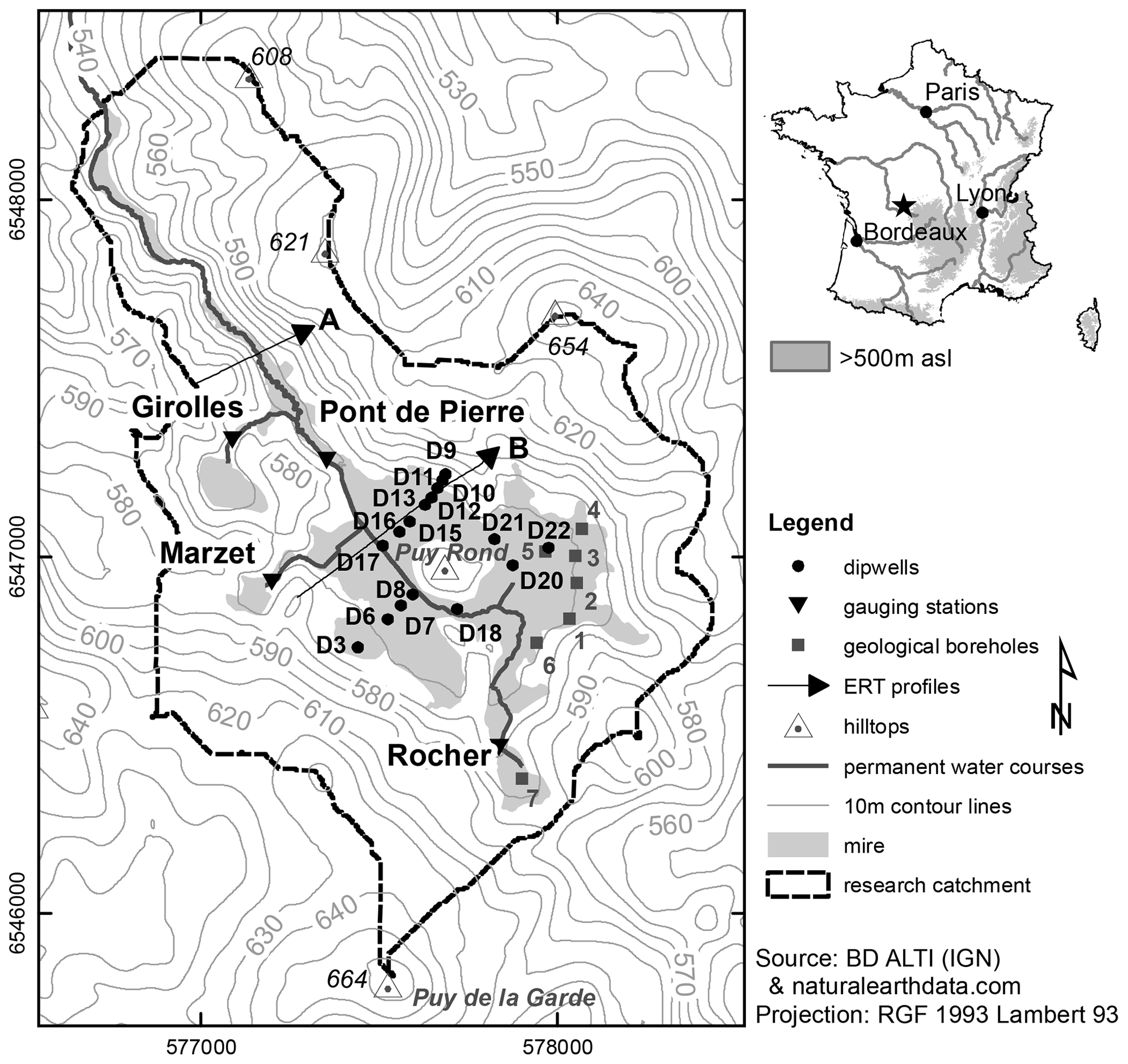
Figure 1The Dauges mire, its catchment and the hydrological monitoring network.
2.2 Hydrometeorological monitoring
Groundwater level was monitored from December 2010 to October 2013 in a network of 16 shallow dipwells installed within the mire and on the lower mineral slopes (Fig. 1). These were equipped with automatic loggers (Mini-Diver, Schlumberger) during all or part of the monitoring period. The 15 min records were corrected for atmospheric pressure recorded by a barometric logger (Baro-Diver, Schlumberger) installed at the site and for logger drift based on regular manual checks and aggregated to daily mean values (Duranel, 2015).
Discharge was measured from January 2011 to December 2013 at the outlet of the main mire area (Pont de Pierre, Fig. 1) using an Orpheus-Mini (OTT) level logger. The 15 min stage records were corrected for logger drift based on regular manual checks and converted to discharge on the basis of a rating curve established from spot discharge measurements undertaken using dilution gauging or an electromagnetic flowmeter and the velocity–area method (Duranel, 2015). Discharge was also measured using sharp-crested V-notch weirs and float loggers (Thalimèdes, OTT) from January 2011 to June 2013 at three locations in the upper reaches of the mire (Girolles, Marzet and Rocher, Fig. 1). Stage records were corrected for logger drift, converted to discharge using the equation provided by Dingman (1994, p. 544) and aggregated to daily mean flow.
Radiation, air temperature, relative humidity, wind speed and rainfall were measured 2 m above ground at the centre of the mire using an Enerco 404 (Cimex) meteorological station from June 2010 to March 2013. Generalised least-square regression models were used to reconstruct long-term (1 August 1998–31 December 2013) daily meteorological time series based on records from nearby Météo-France permanent weather stations, including a station located 4.2 km from the centre of the research site. The reconstructed dataset was used to extend the observed time series and infill missing records (Duranel, 2015). Reference evapotranspiration (ETo) was calculated using the FAO Penman–Monteith method (Allen et al., 1998).
2.3 Geological model
A 3D geological model was built based on a range of field investigations including topographic surveying, geological drilling, electrical resistivity tomography, manual augering and probing, and analysis of existing outcrops. This model is detailed in Duranel (2015) and is summarised here.
Three different datasets were aggregated to produce a digital elevation model (DEM). Within the mire, surface elevation was measured using a differential geo-positioning system (DGPS) at approximately 5 m resolution and with a vertical accuracy of around 10 cm. On mineral soils in the southernmost part of the catchment, topographic data were extracted from the IGN BD Topo, a nationwide DEM with a resolution of 25 m and a root mean square error (RMSE) of 4.8 m against DGPS ground-truthing points within the site. Finally, on mineral soils in the rest of the catchment, the DEM was based on mass points and contour lines at 1 m intervals digitised from existing 1:1000 topographic maps, produced using both traditional surveying and stereo-photogrammetry. Checks carried out using DGPS have shown that the accuracy of mass points is within ±0.1 m.
Electrical resistivity tomography (ERT) was used to estimate the depth of weathered granite formations along three 380 to 868 m long transects across the mire and the lower hillslopes and one 315 m long transect located on the southern hilltop. A detailed description of these profiles is given in Duranel (2015). Figure 2 shows the two most informative profiles, the locations of which are shown in Fig. 1. A Schlumberger configuration was used in both cases, with an electrode spacing of 5 m and a maximum penetration depth of 60 m below ground level. The inversion was performed using the Res2Dinv software (Loke, 2013; Loke and Barker, 1996) and a L1 norm optimisation, leading to RMSEs of 5.3 % for Profile A and 2.2 % for Profile B. Both profiles are characterised by strong contrasts in resistivity values. The most striking feature is the presence on each side of the profiles of highly resistive material overlaying more conductive material. Highly resistive material is only recorded beneath mineral soils on hilltops and slopes and does not occur beneath the mire. The transition between these layers is very sharp, its altitude is largest beneath hilltops, and its depth greatest beneath steep slopes. Out of the four ERT profiles, the only location where conductive material was recorded above resistive material is on one hilltop (visible on the left-hand side of Profile A). These observations were interpreted as demonstrating that most of the material investigated corresponds to the fissured layer of a truncated weathered granite profile. Highly resistive and conductive materials correspond to the unsaturated and saturated fissured layers, respectively. Taking into account the ERT positional accuracy, the margins of the mire coincided on all transects with the location where the inferred groundwater table reaches the ground surface, suggesting a determining role of groundwater seepage in the mire water balance and a high degree of hydrological connectivity between the mire and the fissured layer. The increase in resistivity with depth at the very bottom of Profile B at a depth of around 55 m below ground level was interpreted as a decrease in fissure density (and therefore bulk porosity) and a transition towards unweathered granite. The shallow (less than 2 m deep) superficial layer of conductive material on the hilltop on the left-hand side of Profile A is consistent with (probably unsaturated) saprolite, which is more conductive than the fissured granite layer due to its larger clay and water contents (Baltassat et al., 2005). This configuration was not seen anywhere else within the study area, leading to the conclusion that on most hilltops and hillslopes the majority of saprolite has been eroded away and the combined thickness of the soil, periglacial deposits and remaining in situ saprolite is too small (less than a metre) to have been detected during the ERT survey. There is no indication of the presence of a substantial saprolite layer in the valley bottom beneath the mire; however, the complete saturation of the profile may make the distinction between fissured granite and saprolite impossible in this area.
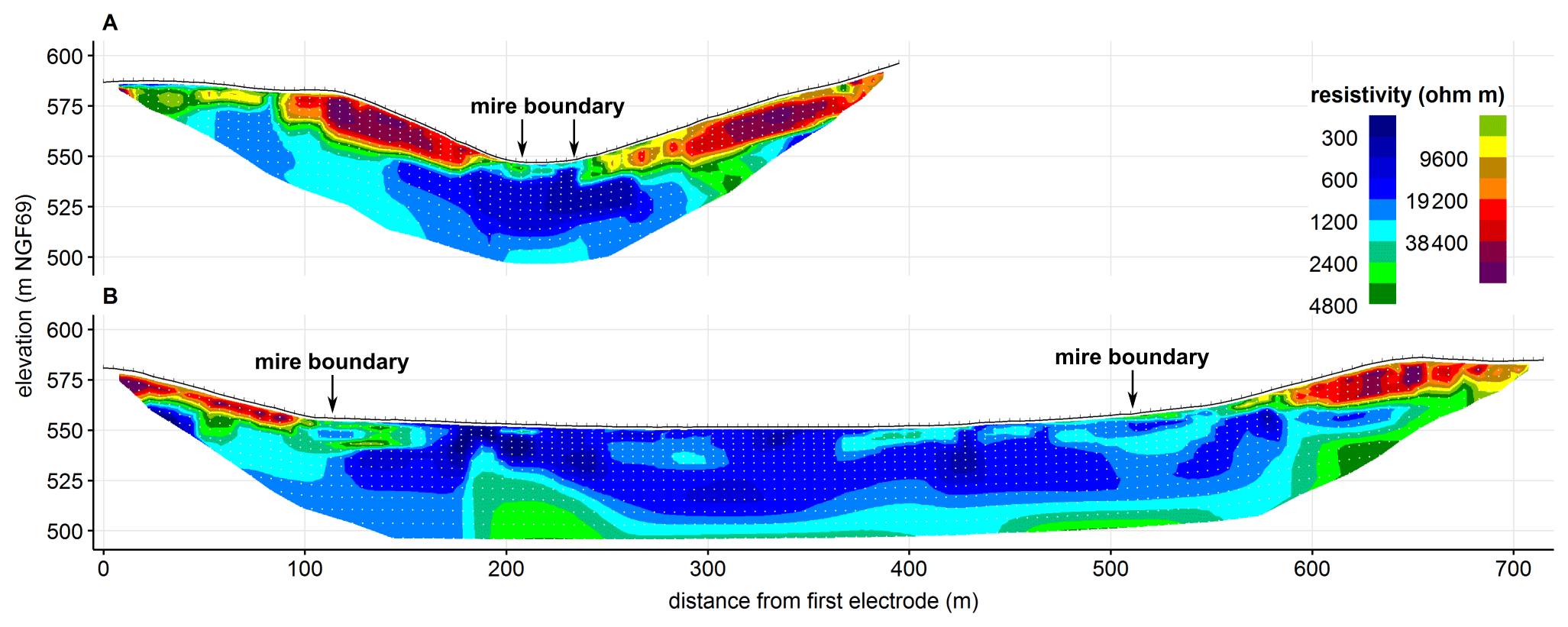
Figure 2Electrical resistivity tomography images obtained after the inversion of apparent resistivity data acquired using a Schlumberger configuration. The survey was conducted using 80 electrodes for Profile A and 144 electrodes for Profile B, with an electrode spacing of 5 m. The inversion was performed using the Res2Dinv software and a L1 norm optimisation, leading to RMSEs of 5.3 % for Profile A and 2.2 % for Profile B. White dots show the centres of model blocks, the black line the surface topography and the black vertical marks the electrode positions. The profile locations are shown in Fig. 1.
Large-scale underground uranium mining was undertaken in the area during the second part of the 20th century. Logs of seven geological boreholes drilled in 1973 by the Commissariat à l'Energie Atomique for the purpose of uranium exploration were provided by the mining company Areva (now Orano). These were all drilled along the eastern margin of the mire, across presumed mineralised faults located using ground surface radiological surveys. They were drilled at an angle of 49.5∘ relative to a horizontal plane to depths of between 67 and 173 m. We used the degree of weathering (assessed on a six-class scale) and the core recovery percentage recorded at the time (Fig. 3) to estimate the depth of the saprolite and of the fissured layer at those locations. The superficial “grus” layer corresponds to saprolite, whereas granite recorded as “weathered” to “highly weathered”, with dense fissuring leading to low or variable core recovery percentages, corresponds to the fissured layer. In line with ERT observations, the depth of the fissured layer ranges from 15 to 65 m and its thickness from 38 to 65 m, with an average of 54 m. Again in line with ERT results, saprolite is absent from the upper part of the catchment (Borehole 7) and from steep slopes surrounding the mire (Borehole 1). However, a substantial saprolite layer 15–40 m deep is present in other boreholes located further inside the mire or on shallower slopes north-east and upstream of Puy Rond. This is seemingly at odds with the apparent absence of saprolite beneath the mire on ERT profiles, located downstream of Puy Rond. It should be noted that the geological boreholes are not representative of the entire catchment as they were drilled within a small area along uranium-rich mineralised faults of tectonic origin, which may have led to a deeper weathering front locally. Another explanation may be that the presence of Puy Rond, by creating a topographic bottleneck, has led to different saprolite erosion rates upstream and downstream of the hill.

Figure 3Geological boreholes drilled by the Commissariat à l'Energie Atomique, showing the granite weathering grade and the core recovery percentage. The borehole locations are shown in Fig. 1. The “highly weathered” and “weathered” layers were interpreted as corresponding to the fissured layer, while the “slightly weathered” to “unweathered” layers were interpreted as corresponding to the bedrock.
Our interpretation of the ERT and geological data agrees with the current understanding of granite weathering processes, granite landscape geomorphology and granite hydrogeology in the Massif Central in general and in the Monts d'Ambazac specifically (Desire-Marchand and Klein, 1986; Dewandel et al., 2006; Godard et al., 2001; Klein, 1978; Klein et al., 1990; Mauroux et al., 2009). The absence of substantial saprolite formations from hilltops and slopes, and presumably from the downstream part of the valley, is in line with Mauroux et al. (2009), who used airborne spectral radiometry to demonstrate that saprolite has been largely eroded away in the Monts d'Ambazac.
Existing sections cutting through periglacial deposits and weathered formations and resulting from small-scale grus extraction or from road construction were also described (Duranel, 2015). These investigations showed that periglacial deposits are very patchy, thin where they occur, and can be considered to be hydrodynamically equivalent to in situ saprolite. Pedological pits dug by Verger (1998) and Gratia (2012 in Duranel, 2015) showed that soils outside the mire are generally relatively deep (40–70 cm), even on hilltops and relatively steep slopes such as those found on Puy Rond. According to the French pedological classification (Baize and Girard, 2009), they mostly belong to acidic podzosols ocriques, allocrisols and brunisols. Texture is loamy-sandy to sandy-gravelly, and drainage is always good.
Peat deposits were mapped using manual augering and probing. The average peat depth within the mire was 0.80 m (standard deviation 0.49 m), with a maximum of 3.45 m at its centre (Duranel, 2015). Stratigraphical surveys and slug tests showed a rapid increase in peat humification and a decrease in hydraulic conductivity with depth, which is consistent with observations from many mires worldwide. Ingram (1978), based on concepts developed by Ivanov (1953) and Romanov (1968), proposed the definition of “acrotelm” as the upper layer characterised by a low humification and high hydraulic conductivity and porosity, and “catotelm” the lower layer with the opposite characteristics. At the Dauges site, peat hydraulic conductivities measured between 0.1 and 0.2 m below ground level had a median value of m s−1. Values recorded at depths ranging from 0.6 to 1.5 m below ground level were 2–3 orders of magnitude smaller (median value: m s−1). The depth of the acrotelm (based on the pedological definition of van der Schaaf, 1999, 2002) was generally smaller than 25 cm. However, these field investigations also demonstrated that peat properties were highly variable across the site. Alluvial deposits of sand and small gravel, up to 1.7 m thick, were found beneath the peat along the stream downstream of Puy Rond. Further away from the stream, similar material was found to form 10 to 110 cm thick patchy lenses intermixed with peat deposits.
2.4 Hydrological model development
The MIKE SHE/MIKE 11 modelling system (Graham and Butts, 2005; Refsgaard et al., 2010) was used to model the mire and its catchment. MIKE SHE/MIKE 11 is a deterministic, fully distributed modelling system able to model actual evapotranspiration, unsaturated zone flow and storage, saturated zone flow and levels, overland flow and channel flow processes in an integrated manner. It has previously been successfully applied in a wide range of wetland environments (e.g. Al-Khudhairy et al., 1999; Bourgault et al., 2014; Clilverd et al., 2016; Hammersmark et al., 2010; House et al., 2016a; Thompson, 2004; Thompson et al., 2004, 2017). Originally fully physics-based, it has evolved to include a suite of modules that also allow for the use of simplified physical equations or even conceptual models based on distributed, semi-distributed or lumped approaches (Refsgaard et al., 2010). In the present study, a combination of both physics-based and conceptual modelling approaches was used. A 10 m × 10 m grid was employed throughout the model, resulting in 23111 model cells.
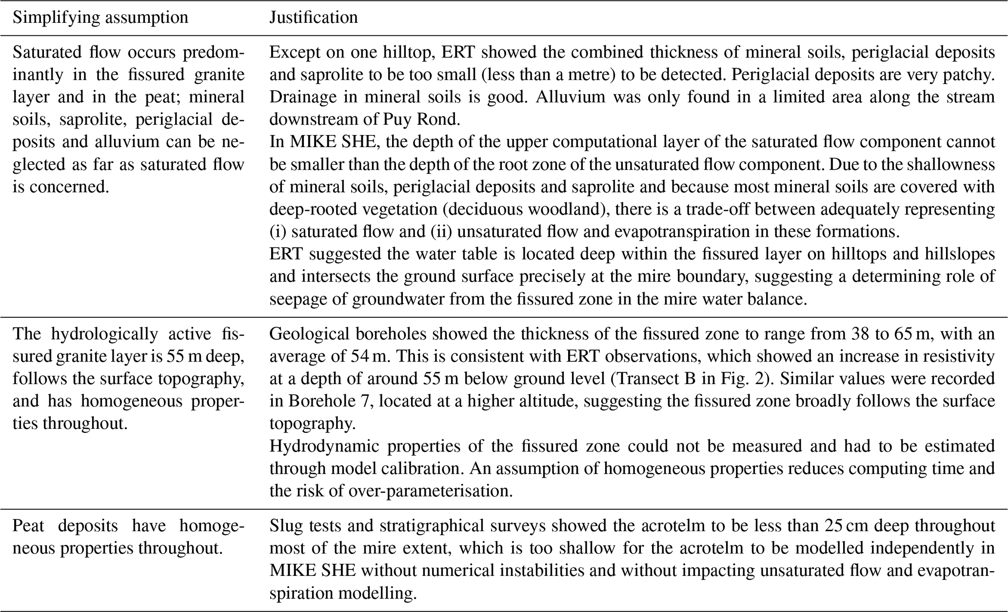
Saturated flow was modelled using an iterative implicit finite-difference technique to solve the 3D Darcy equation including within the fissured granite for which an equivalent porous medium approach (Long et al., 1982) was used. In the development of the saturated flow model, we used the most plausible geological conceptualisation based on the data detailed in Sect. 2.3 while making a number of reasonable simplifying assumptions to account for constraints associated with practical computing times, available data and the risk of over-parameterisation. These assumptions, further justified in Table 1, were that (i) saturated flow occurs predominantly in the fissured granite layer and in the peat; (ii) mineral soils, saprolite, periglacial deposits and alluvium can be neglected as far as saturated flow is concerned; (iii) the hydrologically active fissured granite layer is 55 m deep, follows the surface topography, and has homogeneous properties throughout; and (iv) peat deposits have homogeneous properties throughout.
Table 1Justification of simplifying assumptions of the saturated flow model component.
Only two geological formations (peat and fissured granite) were therefore represented in the saturated flow model, with peat only occurring within the mire extent. The saturated flow model was nevertheless divided into two computational layers throughout the model extent, because MIKE SHE does not allow for discontinuous computational layers. Throughout the model, the lower layer represented the fissured granite, with a constant depth of 55 m below the topographic surface. Outside of the mire, the upper computational layer had identical properties to the lower layer and also represented the (upper) fissured granite. In MIKE SHE the depth of the upper computational layer of the saturated flow component cannot be smaller than the depth of the root zone in the unsaturated flow component. Therefore, outside of the mire, the upper layer was defined as 2 m deep to match the estimated root depth of woodlands. Within the mire, where shallow-rooted open vegetation dominates, the upper layer represented peat deposits. Its depth followed that measured in the field, with a minimum value of 0.5 m to avoid numerical instabilities. A no-flow boundary was assumed around the boundaries of the topographic catchment. At the downstream end of the catchment, a constant-gradient boundary was used, assuming that the slope of the phreatic surface broadly follows that of the topographic surface. Overland flow was modelled using a 2D, finite-difference, diffusive wave approximation of the Saint-Venant equations, solved using the successive over-relaxation method.
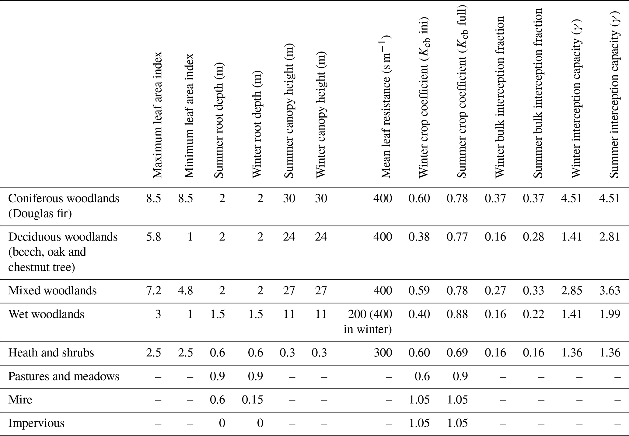
The empirical two-layer unsaturated zone model (Yan and Smith, 1994) was selected. This was principally to reduce computation time but was also justified by the lack of detailed data on unsaturated zone properties since the lower number of parameters required by the two-layer model facilitates their estimation through calibration. Due to the two-layer model's limitations in representing interception in woodland, evaporation from interception was modelled outside MIKE SHE using the same equations as those implemented in the HYLUC model (Calder, 2003), with a distinction being made for tall vegetation (woodland, heath and shrubs) between wet-time evaporation (corresponding to evaporation from interception, modelled outside MIKE SHE) and dry-time evapotranspiration (which includes transpiration and any other evaporation from the ground surface, simulated using MIKE SHE's two-layer model). Calder's γ parameter was calibrated against the mean of bulk interception ratios (annual for evergreen conifers and heathlands, seasonal for deciduous woodlands) cited in the literature for similar vegetation types and measured in similar climatic conditions (Delgado et al., 2010). The method proposed by Allen et al. (1998) and Allen and Pereira (2009) was used to estimate the basal crop coefficient Kcb (equivalent to Calder's β) based on climate, vegetation height, leaf area index and mean leaf resistance. As recommended by Calder (2003), no distinction was made between wet-time evaporation and dry-time evapotranspiration for short vegetation (grassland and mire), and therefore evapotranspiration was fully modelled within MIKE SHE. Crop coefficients for short vegetation types were taken from the literature. The values used for parameterising the evapotranspiration model are shown in Table 2.
The MIKE SHE model was coupled to a MIKE 11 1D river model of the main channels within the catchment. In order to achieve logistically feasible run times during calibration and validation, channel flow was modelled using a kinematic routing method and water levels estimated a posteriori based on Manning's equation. This method is fast and generally relatively accurate for fast-flowing streams where no backwater occurs (DHI, 2009b). It is not expected to give an accurate representation of stream stage, and as a consequence it was assumed that exchanges between the overland flow component and watercourses occur towards the latter only (i.e. there is no over-bank flooding). This simplification is acceptable since within the research site over-bank flooding only occurs within a very narrow band along the main stream and in a limited area in the downstream part of the mire.
The Dauges MIKE SHE/MIKE 11 model used an adaptive time step, whilst results were aggregated to a daily resolution. Model outputs were extracted for the period 1 January 2001–31 December 2013, after an approximately 2.5-year warm-up period beginning on 1 August 1998 (corresponding to the installation of the nearest permanent automatic meteorological station).
2.5 Hydrological model calibration and validation
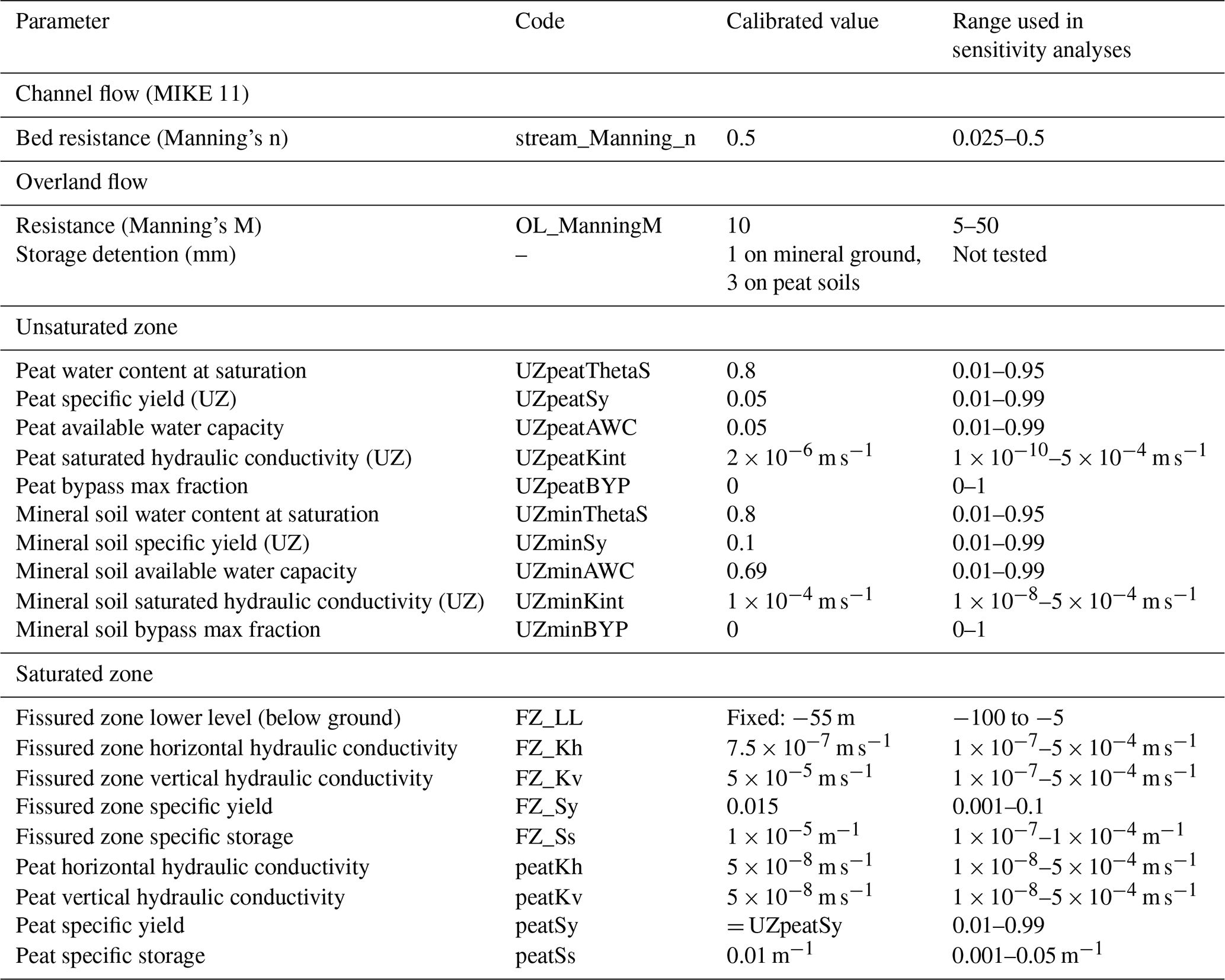
The model was manually calibrated and validated against observed discharges and groundwater table depths. To accommodate slightly different data availabilities, the calibration period was set as 1 January 2011–30 June 2012 for discharge and 1 January 2011–31 December 2012 for groundwater table depth. The validation period was set as 1 July 2012–31 December 2013 for discharge and 1 January–31 December 2013 for groundwater table depth. Model performance was evaluated using the Nash–Sutcliffe efficiency (NSE) and percent bias (PBIAS) statistics recommended by Moriasi et al. (2007) and a visual assessment of the ability of the model to reproduce seasonal groundwater table patterns. Calibration parameters together with their calibrated values are shown in Table 3.
Table 3Calibration parameters of the MIKE SHE/MIKE 11 model of the Dauges catchment, including their final values and the range used in sensitivity analyses.
The ability of the calibrated model to simulate realistic groundwater tables across the catchment was further investigated by validating a raster map of the mean groundwater table depth simulated across the site for the 2001–2013 period against the observed mire boundaries, mapped using a combination of botanical (Durepaire and Guerbaa, 2008) and pedological (Duranel, 2015) criteria. The groundwater table depth threshold best discriminating between mire and other habitats was found by optimising a Cohen's kappa agreement function (Congalton, 1991) between simulated and observed mire boundaries.
2.6 Sensitivity analysis
The local sensitivity of the model around the calibrated parameter values was evaluated by assessing the rate of change in the root mean square error for simulated discharge and groundwater table depth when a single parameter was perturbed by a defined proportion (Rochester, 2010). The sensitivity of the model to a parameter i is calculated following Eq. (1):
where θi is the model parameter investigated, and θi, upper and θi, lower are the user-specified upper and lower limits of the parameter (see Table 3). Scaling by the parameter range allowed for the comparison of local sensitivity coefficients between parameters of different scales of magnitude. The sensitivity was evaluated locally around the calibrated parameter values (θ1, θ2, … , θn), only one of which (θi) was perturbed. A perturbation fraction of 5 % of the range was used, implementing both the backward and forward difference approximation methods (DHI, 2009a). The sensitivity of the model to the depth of the granite fissured zone was also tested, although this parameter was not used for calibration.
2.7 Water balance analysis
A water balance was computed using the MIKE SHE water balance tool for two areas upstream of the main mire outlet corresponding to mineral and peat soils, respectively. These water balance domains cover 36.9 and 125.0 ha, respectively (Fig. 4). The water balance was not calculated over the entire model domain for two reasons: firstly to reduce potential errors caused by uncertainty in boundary conditions at the north-western end of the model domain as well as the relatively sparse hydrogeological and hydrological data downstream of Pont de Pierre; and secondly to constrain the focus of the analysis on the main designated mire area upstream of Pont de Pierre. The stream flowing through the mire was not included in the water balance of the mire (i.e. only fluxes between the stream and peat soils or the surface of the mire were considered, with flow in and out of the stream where it enters and exits the mire excluded).

Figure 4Water balance domains used within the MIKE SHE/MIKE 11 model of the Dauges catchment.
Simulated groundwater table depth, upward saturated flow from the lower computational layer (hereafter referred to as groundwater upwelling) and exchange from the saturated zone to overland flow (hereafter referred to as groundwater seepage) were mapped across the entire catchment.
2.8 Processes driving changes in groundwater table depth in peat soils
Processes driving changes in groundwater table depth in peat soils were investigated using variation partitioning (Legendre and Legendre, 1998), based on simulated spatially averaged monthly means to focus on timescales relevant to vegetation (Wheeler et al., 2004). Explanatory variables included precipitation, groundwater upwelling, overland boundary inflow, actual evapotranspiration and groundwater table depth in the preceding month. An exploratory analysis showed that the relations between groundwater table depth and explanatory variables were mostly non-linear; therefore, variation partitioning was undertaken in a generalised additive modelling (GAM) framework (Wood, 2016).
3.1 Model performance
Figures 5 and S1 in the Supplement show observed and simulated daily discharge at the four gauging stations during the calibration and validation periods. According to the guidelines of Moriasi et al. (2007), model performance with regard to discharge at the mire outlet (Pont de Pierre) was good to very good (NSE close to 0.75 during both calibration and validation and overall, percent bias lower than ±10 % overall). Both high and low flows were well reproduced. Performance was not as good for the smaller upstream reaches, with the model slightly underestimating total discharge and predicting flashier patterns compared to those observed. However, performance was still classified as satisfactory (overall NSE >0.5).

Figure 5Observed and simulated stream discharge and model performance statistics for two selected locations within the Dauges catchment (1 January 2011–31 December 2013). Note different y-axis ranges.
Model performance with regard to groundwater levels was variable (Figs. 6 and S2). It should be assessed relative to the site's topography: the altitude range from the bottom of the mire to the top of the hills surrounding it and delineating the model boundaries is 110 m. The performance was therefore clearly good to very good for a large number of dipwells (such as D7, D13, D15, D18, D20 and D21) for which RMSEs of the order of ≤ 10 cm and NSEs of between 0.55 and 0.85 were achieved. In these dipwells, all located within the mire some distance from the stream and the mire margins, the seasonal patterns were well reproduced. This was the case for instance in Dipwell D7, at the centre of the mire, where the surface saturation in winter, the drop in groundwater level in late spring or early summer and the rapid fluctuations caused by summer precipitation events were clearly reproduced. The slight underestimation of groundwater levels in winter and spring was more a reflection of the difficulties in accurately defining ground level in peatlands (Dettmann and Bechtold, 2016) than a modelling issue (this is further discussed in Sect. 4.2).
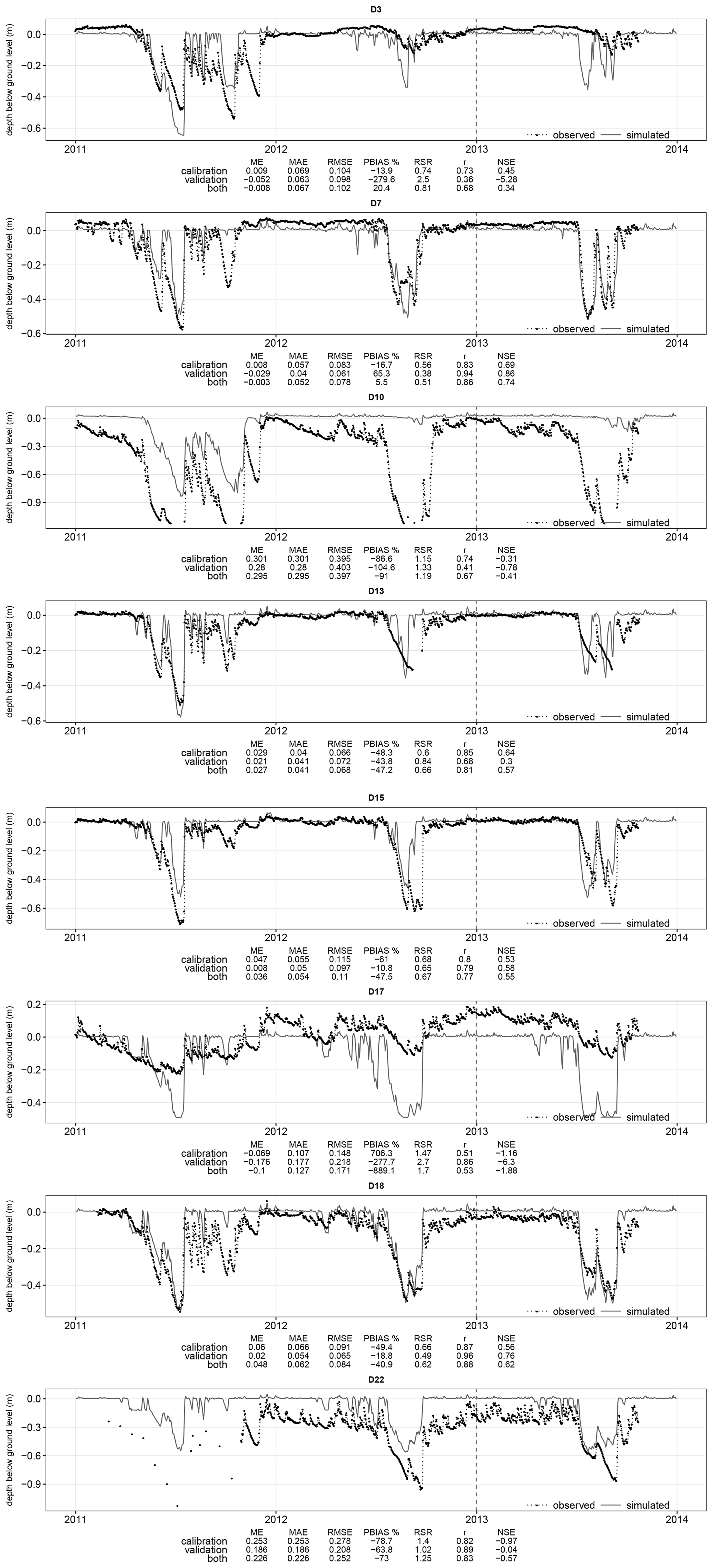
The model performance was less good, but still satisfactory, for some dipwells (e.g. D3, D9 and D10) which are close to the mire boundary or within the mineral soils just outside it. In D3 for instance, the much shallower groundwater table levels observed in 2012 and 2013 compared to 2011 were not very well reproduced. Conversely in D10, simulated levels were too shallow during the summers of 2012 and 2013. Dipwells D3, D9 and D10 are located where discrepancies between the actual ground elevation of the observation point and that interpolated at the corresponding DEM grid cell are the largest. This is a result of the relatively steep slopes, and it is at these locations that the approximations caused by the model discretisation are the largest. During calibration, it became evident that simulated water table depths at these dipwells were more sensitive to the parameterisation of the fissured zone than those located at the centre of the mire. While it was possible to improve the fit for dipwells on one side of the mire, this improvement was balanced by deterioration in performance for dipwells located on the other sides. This may be explained by the fact that the fissured zone was modelled as a homogeneous layer, which facilitates calibration and reduces the risk of over-parameterisation at the model scale but does not allow for fine-scale adjustment to local variations in hydrodynamic properties (see Sect. 4.1).
Relatively poor performance was achieved for dipwells located close to the stream in the lower part of the mire (D8, D16, D17). Dipwells D16 and D17 are inserted into highly permeable alluvial gravel beneath or within the peat along the stream, and as a consequence groundwater table in these dipwells is largely driven by water levels in the nearby stream. The poor performance of the model in these locations was therefore a direct consequence of the absence of alluvial deposits in the model and the likely poor simulation of water levels in watercourses resulting from the kinematic routing method (Duranel, 2015). Finally, performance was poor for Dipwell 22 as a consequence of the presence of a 30 cm deep superficial layer of oxidised peat in this part of the mire resulting from historical agricultural drainage. This layer was not represented in the model due to its small extent and depth, and, as a result, the deeper and more variable observed groundwater level was not adequately simulated (Fig. 6). However, both the oxidised peat and the gravel deposits occupy only a small proportion of the mire extent, and their impact on the overall model performance is therefore considered to be small.
The model predicts the observed extent of mire habitats very well. The long-term mean annual groundwater level threshold that best discriminates between mire and non-mire habitats was found to be 0.166 m below ground level. This gives a value for Cohen's kappa agreement function of 0.841, corresponding to 95.0 % of grid cells being correctly classified (Table 4, Fig. 7). The good match between observed and simulated mire boundaries was not only observed within the main extent of the mire, but also along the narrow valley downstream and in the small sub-basins upstream (locations labelled (b), (d), (g) and (h) in Fig. 7). These small basins are located 10–30 m above the main mire, suggesting that the model simulates groundwater levels well even in the upper part of the catchment where no groundwater level time series were available for calibration. Small, localised discrepancies between the observed and simulated mire boundaries may be explained by different factors. Some false positives (grid cells wrongly predicted to support mire vegetation) may in part be due to errors in the mire vegetation map itself, for instance along the narrow valley in the north-east of the catchment (location (a) in Fig. 7) where difficult access and tree cover may have hindered mapping efforts. Location (c) coincides with relatively large errors produced by the MIKE SHE overland flow component. DEM inaccuracies may explain discrepancies at locations (e) and (f) along the south-eastern margin of the mire, since this area corresponds to the boundary between the low-resolution, low-accuracy IGN BD Topo DEM on the south-eastern hillslopes and the high-resolution, high-accuracy DGPS DEM within the mire.
Table 4Confusion matrix between the observed mire distribution based on botanical (Durepaire and Guerbaa, 2008) and pedological (Duranel, 2015) criteria and the predicted mire distribution based on model results (simulated mean annual groundwater level >0.166 m below ground level for the period 2001–2013), in % of the total number of grid cells.
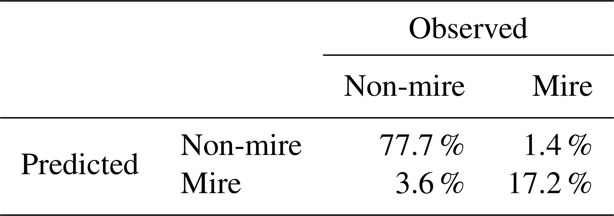
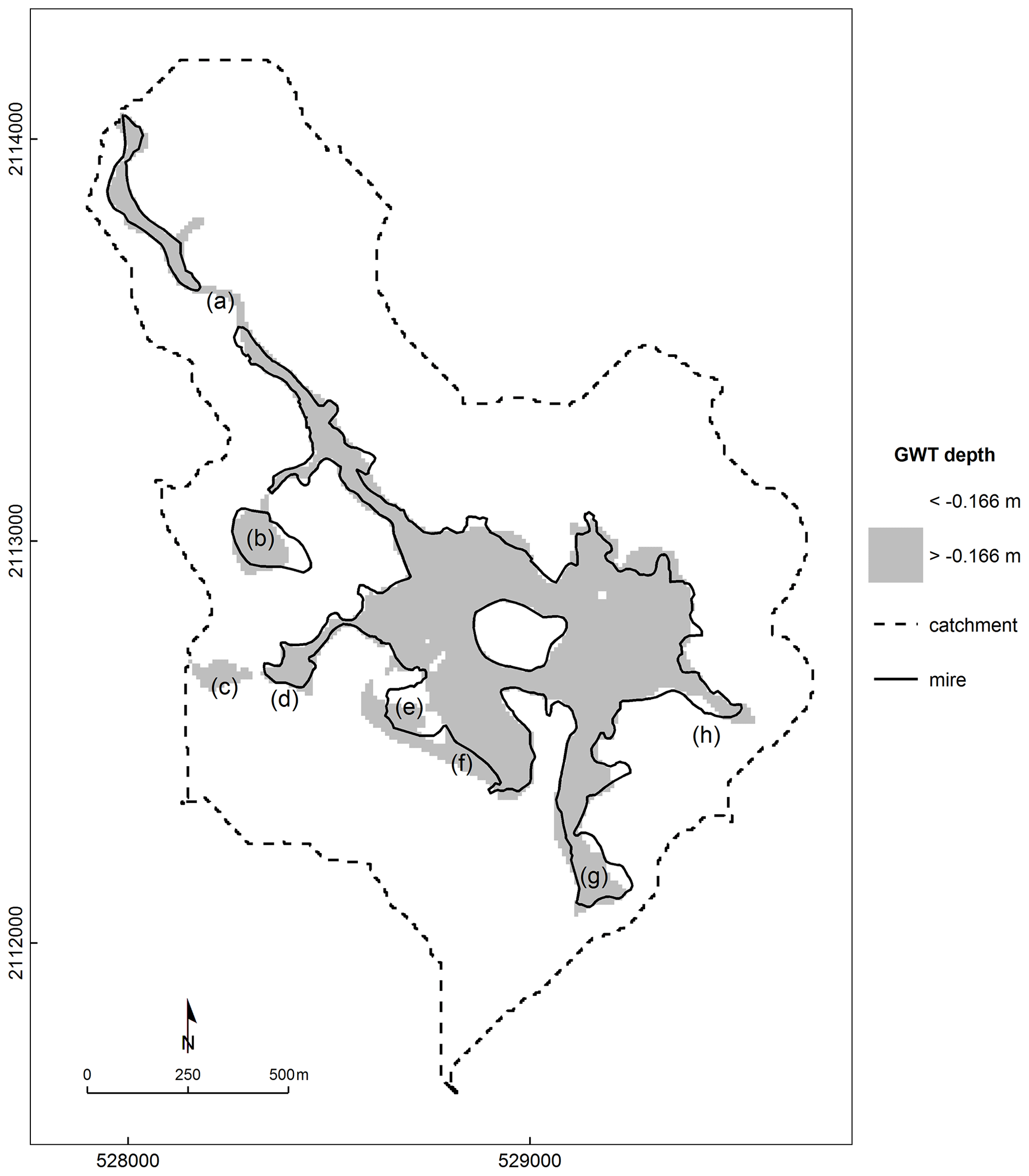
Figure 7Observed mire boundary based on botanical (Durepaire and Guerbaa, 2008) and pedological (Duranel, 2015) criteria and the predicted mire distribution based on model results (simulated 2001–2013 mean groundwater table depth higher than 0.166 m below ground level). (a–h) refer to locations discussed in the text (see Sect. 3.1).
Nevertheless, despite the issues discussed above, the satisfactory to very good performance at a large number of monitoring locations for both discharge and groundwater table depth and the excellent fit between observed and simulated mire boundaries suggest that the model reproduces the dominant hydrological characteristics of the mire, including its water balance which is discussed below.
3.2 Local sensitivity of the calibrated model
Figure 8 provides the mean absolute scaled sensitivity coefficient for each model parameter that was tested with respect to groundwater level, discharge at the mire outlet (Pont de Pierre in Fig. 1) and discharges of the small upstream reaches (Girolles, Marzet and Rocher in Fig. 1). The parameters to which the calibrated model is most sensitive with regard to groundwater level are first and foremost those related to the hydrological characteristics of mineral formations: the horizontal saturated hydraulic conductivity, the depth and specific yield of the fissured zone, and the available water capacity of the unsaturated mineral soils. This is the case whether dipwells are located on mineral soils or within the mire. The peat parameter to which the model is most sensitive is the vertical saturated hydraulic conductivity, which controls upwelling/downwelling fluxes between the peat layer and the underlying mineral formations.
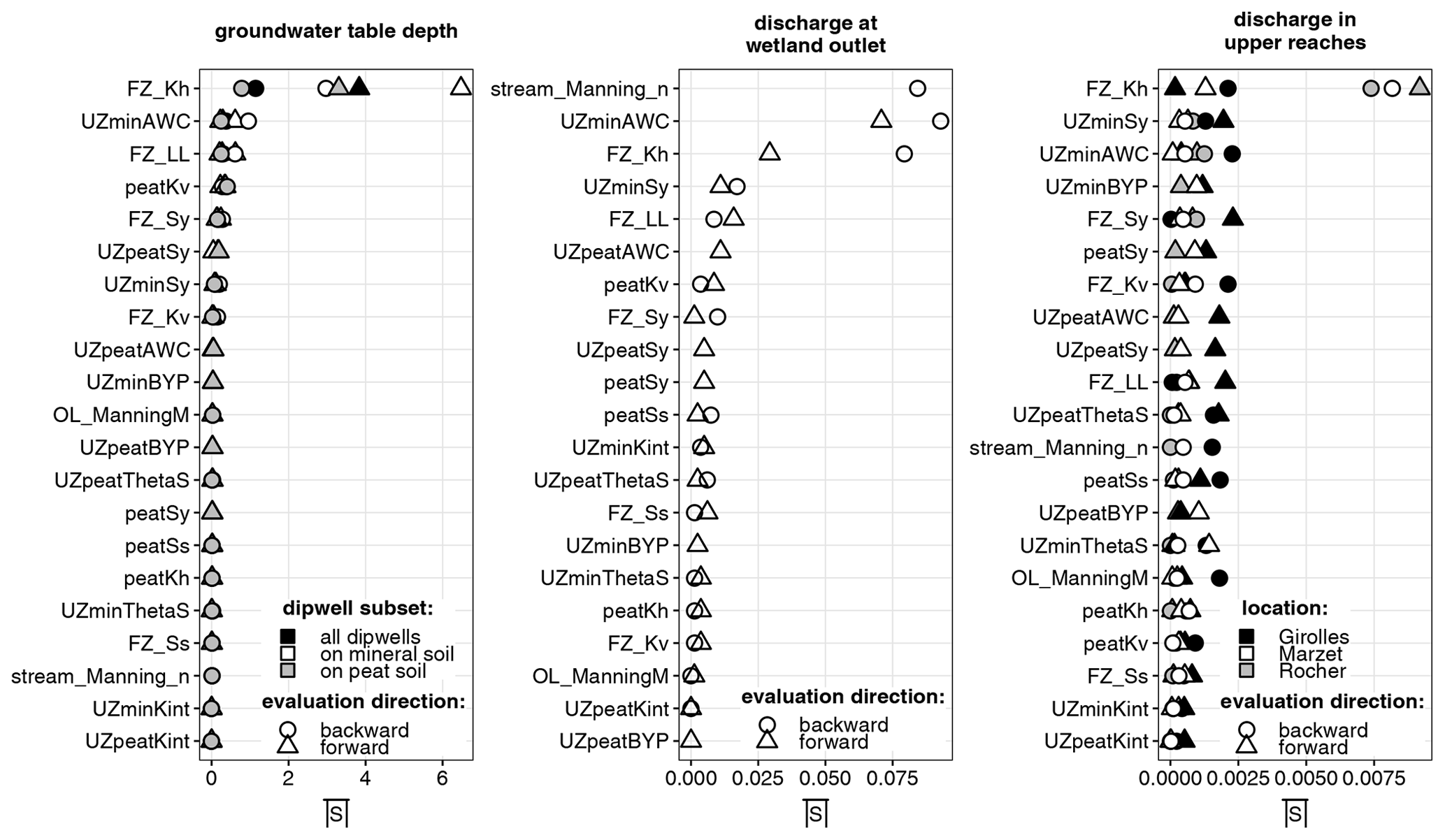
Figure 8Summary of model sensitivity analysis results (see Table 3 for parameter codes). Parameters are arranged in order of increasing mean sensitivity from bottom to top.
The horizontal saturated hydraulic conductivity of the fissured zone is also the parameter to which simulated discharges of upstream reaches are by far most sensitive. Other influential parameters determine unsaturated flow in mineral soils: specific yield, available water capacity and the bypass fraction. Discharge at the mire outlet is also strongly influenced by parameters describing fluxes in mineral formations: available water capacity and specific yield in mineral soils and horizontal saturated hydraulic conductivity and depth of the fissured zone. Stream Manning's n is also very influential. Parameters describing the peat layer are less important.
3.3 Mire water balance
Figure 9 shows the simulated long-term (2001–2013) mean annual water balance of the mire (corresponding to the peat soil domain in Fig. 4). Detailed water balances of both the peat and mineral soil domains are provided in Table S1. The water balance computational error was 9.9 % of total annual inflows and was almost entirely due to the overland flow component. Extensive attempts were made to reduce this computational error by tightening the convergence criteria; however, this resulted in relatively small gains but a substantial increase in computing time. This is considered to be a minor issue because, as a result of the quasi-constant saturation, very little infiltration is simulated within the mire. Consequently, the overland flow component error mainly affects simulated overland outflow to the river, which is not the main focus of this study and has little impact on other water balance terms. The water balance error within the mineral soils domain was only 1.6 % of total inflows. This is, again, mostly caused by the overland flow component. The three main sources of water to the mire are precipitation (32.1 % of total inflows), groundwater upwelling from the underlying mineral formations (27.1 %), and overland boundary inflow (i.e. non-channelised runoff from the mire catchment). The latter accounts for 40.2 % of total inflows; however, a large proportion of this originates from edge-focused groundwater seepage on mineral soils just upstream of the mire (see Sect. 3.4). Lateral saturated boundary inflows from the mineral catchment and from the river are negligible (0.5 % and <0.0 % of total inflows, respectively). Significantly, groundwater upwelling provides 92.4 % of inputs to the mire saturated zone, which drives groundwater levels. Percolation from the unsaturated zone to the saturated zone (5.3 %) and infiltration from overland to the saturated zone (0.7 %) are only possible when the groundwater table drops below ground level for 2–3 months in summer and early autumn. At all other times, inputs from precipitation and overland boundary flow quickly leave the mire as saturation-excess runoff and so do not contribute to the water balance of the saturated zone.
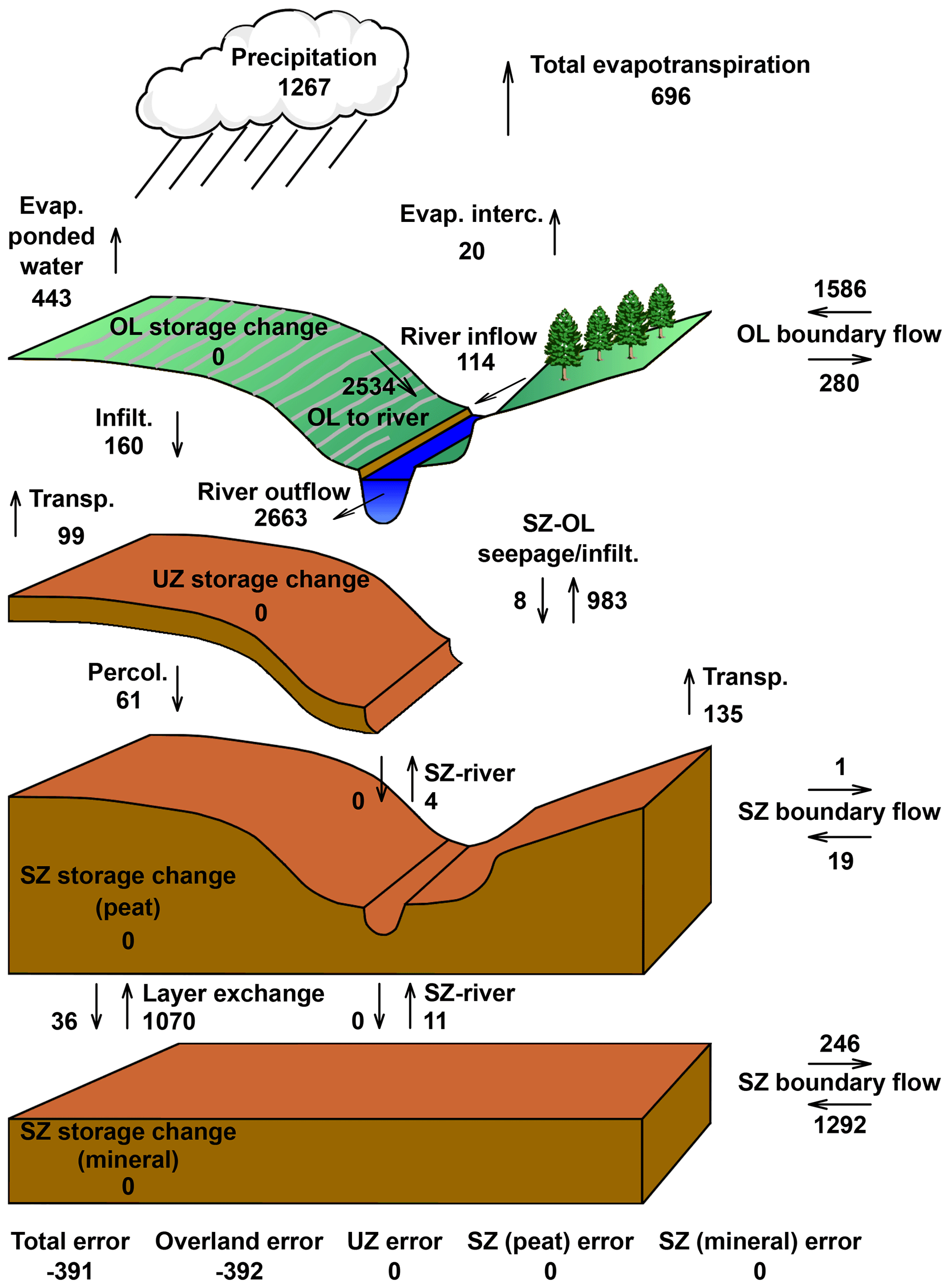
Figure 9Simulated mean annual water balance of the Dauges mire (mm yr−1) for the period 2001–2013. Evap.: evapotranspiration; interc.: interception; transp.: transpiration; infilt.: infiltration; percol.: percolation; OL: overland; UZ: unsaturated zone; SZ: saturated zone.
Figure 10 breaks down the mire's long-term water balance by calendar month. The largest total inflows to the mire occur in winter and early spring. They then gradually decline throughout the spring and summer, reaching a minimum in September. Total outflows, dominated by overland runoff to the stream and to a lesser extent by evapotranspiration, follow the same pattern. Changes in storage are relatively small, reflecting the very shallow groundwater levels and the rapid removal of any water surplus through saturation-excess runoff, particularly in late autumn, winter and early spring. Due to the site's position at the transition between a degraded oceanic climate and a mountainous climate (Joly et al., 2010), precipitation is, on average, relatively well distributed throughout the year, although there is relatively large inter-annual variability. Overland boundary inflow is highly variable seasonally. It reaches its maximum in winter and early spring (accounting for 49.6 % of total inflows in January and February) before gradually declining to a minimum in September (22.9 %). It also exhibits large inter-annual variability, reflecting the similar variability in precipitation. Upward saturated flow from the lower computational layer (i.e. groundwater upwelling) is relatively constant from December to May before gradually declining to reach a minimum in September. It is characterised by much smaller seasonal and inter-annual variabilities than precipitation and overland boundary inflow and, therefore, generally provides a larger proportion of total inflows in summer and early autumn (37.2 % in September, Fig. S3). As noted above, groundwater upwelling accounts for, on average, 92.4 % of total inflows to the mire saturated zone. Seasonally this figure peaks at 95.5 % in January and declines to 88.1 % in August. At this time receding groundwater levels allow for the formation of an unsaturated zone across a larger proportion of the mire and for precipitation and overland boundary inflow to infiltrate and percolate, respectively, instead of producing saturation-excess runoff.
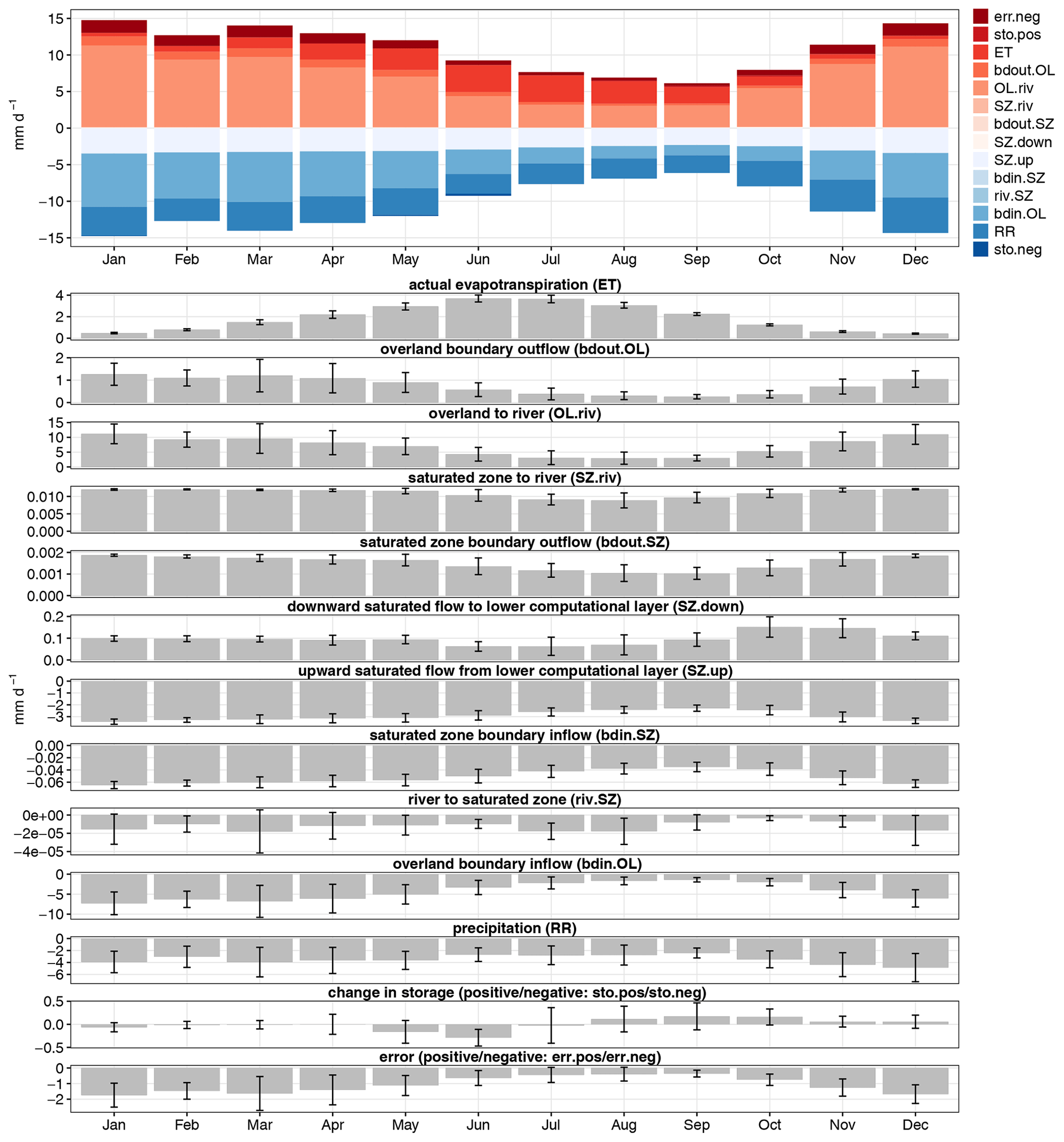
Figure 10Simulated mean monthly water balance of the Dauges mire (2001–2013). Figures follow the MIKE SHE water balance convention: inputs are negative, outputs positive, change in storage positive when storage increases, and the water balance error is the sum of all inputs and outputs. Whiskers show the standard deviation. Top plot: see titles of bottom plots for variable codes.
3.4 Spatial patterns in groundwater table depth and groundwater seepage
Figure 11 shows the spatial distribution of simulated long-term (2001–2013) mean annual groundwater table depth and groundwater seepage rates in January and September when long-term mean seepage rates are highest and lowest, respectively (data for other calendar months are shown in Fig. S4). Spatial and temporal patterns in groundwater upwelling rates are very similar to those in seepage rates and are therefore not shown. As discussed above, the mire boundaries are closely associated with shallow groundwater table depths. Groundwater upwelling and seepage rates are highest along or immediately upstream of the mire boundary. This is a clear example of edge-focused discharge (Richardson et al., 2001), whereby groundwater discharge at the ground surface is enhanced where there is a break in the slope of the surface topography and, consequently, of the water table gradient. The lower topographic slope within the mire itself leads to a rapid decrease in the vertical hydraulic gradient towards the centre of the mire; however, the model suggests that groundwater seepage occurs throughout the mire even in the driest month. The extent of the area where groundwater seepage occurs peaks in January, when it extends largely to mineral soils surrounding the mire and to the small non-channelised valleys and slope breaks in the upper part of the catchment. This area progressively shrinks, reaching its minimum extent in September. It is at this time of the year that the agreement between spatial patterns in simulated groundwater seepage and observed mire boundaries is highest (kappa =0.845). The monthly mean groundwater seepage threshold best discriminating between mire and non-mire vegetation during this calendar month is 0.005 mm d−1, suggesting that the mire boundaries are determined by the presence or absence of groundwater seepage during the driest month of the year. Nevertheless, minor localised discrepancies between observed mire boundaries and simulated groundwater table depth described in Sect. 3.1 are also evident in the spatial patterns of groundwater upwelling and seepage, in particular along the south-eastern boundary of the mire.
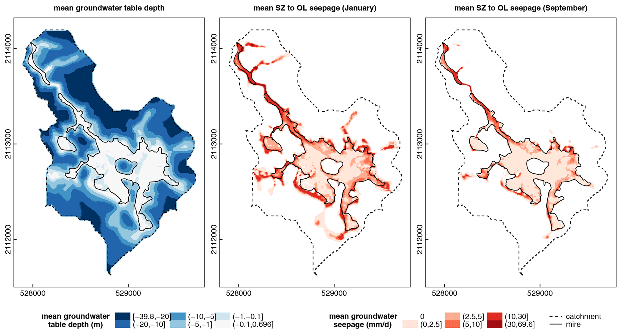
Figure 11Simulated mean annual groundwater table depth and groundwater seepage rates in January and September (2001–2013). SZ: saturated zone; OL: overland.
3.5 Processes driving groundwater table depth in peat soils
Figure 12 shows time series of spatially averaged monthly mean groundwater table depth and selected water balance items in the peat soils. Groundwater table depth shows low inter-annual variability in winter, being consistently within a few centimetres of ground level. Inter-annual variability is larger in summer. The grey bands in Fig. 12 highlight summers with the deepest (2005) and shallowest (2007) mean groundwater tables. These are concomitant with unusually low and high groundwater upwelling rates and overland boundary inflows, which themselves followed relatively dry and wet winters and springs, respectively. Evapotranspiration shows relatively little inter-annual variability, which can be explained by the relatively shallow groundwater table depth within the mire and the absence of water availability limitation. Groundwater upwelling and overland boundary inflow are highly correlated (Spearman's rank correlation =0.973, Fig. S5), the later increasing exponentially with the former, whereas both are only weakly correlated with precipitation. This further demonstrates that most of the overland boundary inflow to the mire originates from groundwater seepage through mineral soils. All terms except overland boundary inflow are significant in a full generalised additive model (Table 5). A reduced model without overland boundary inflow has a lower Akaike information criterion (AIC) than the full model (−597.3 vs. −593.5, respectively). Given the process link between groundwater upwelling within the mire and overland boundary inflow (both related to upward movement of groundwater from the underlying granite), the latter was not used for variation partitioning. Figure 13 shows the smooth terms of the reduced model. It demonstrates that, with all other variables being fixed at their sample mean, groundwater table depth increases linearly with groundwater upwelling up to about 3 mm d−1. Thereafter it reaches a plateau approximately corresponding to ground level. Beyond this level, any additional input is converted to groundwater seepage and overland runoff to the stream and so does not contribute to further increases in groundwater table depth. Similarly, groundwater table depth increases linearly with rainfall up to about 3 mm d−1 before reaching a plateau. It is inversely related to evapotranspiration, but only above ca. 2 mm d−1. Finally, groundwater table depth is linearly (and weakly) related to groundwater table depth in the preceding month.
Table 5Approximate significance of smooth terms in the full generalised additive model.

GWTm−1: monthly mean groundwater table depth in the preceding month; RR: monthly mean precipitation; SZ.up: monthly mean upward saturated flow from the lower computational layer; bdin.OL: monthly mean overland boundary inflow; ET: monthly mean actual evapotranspiration.
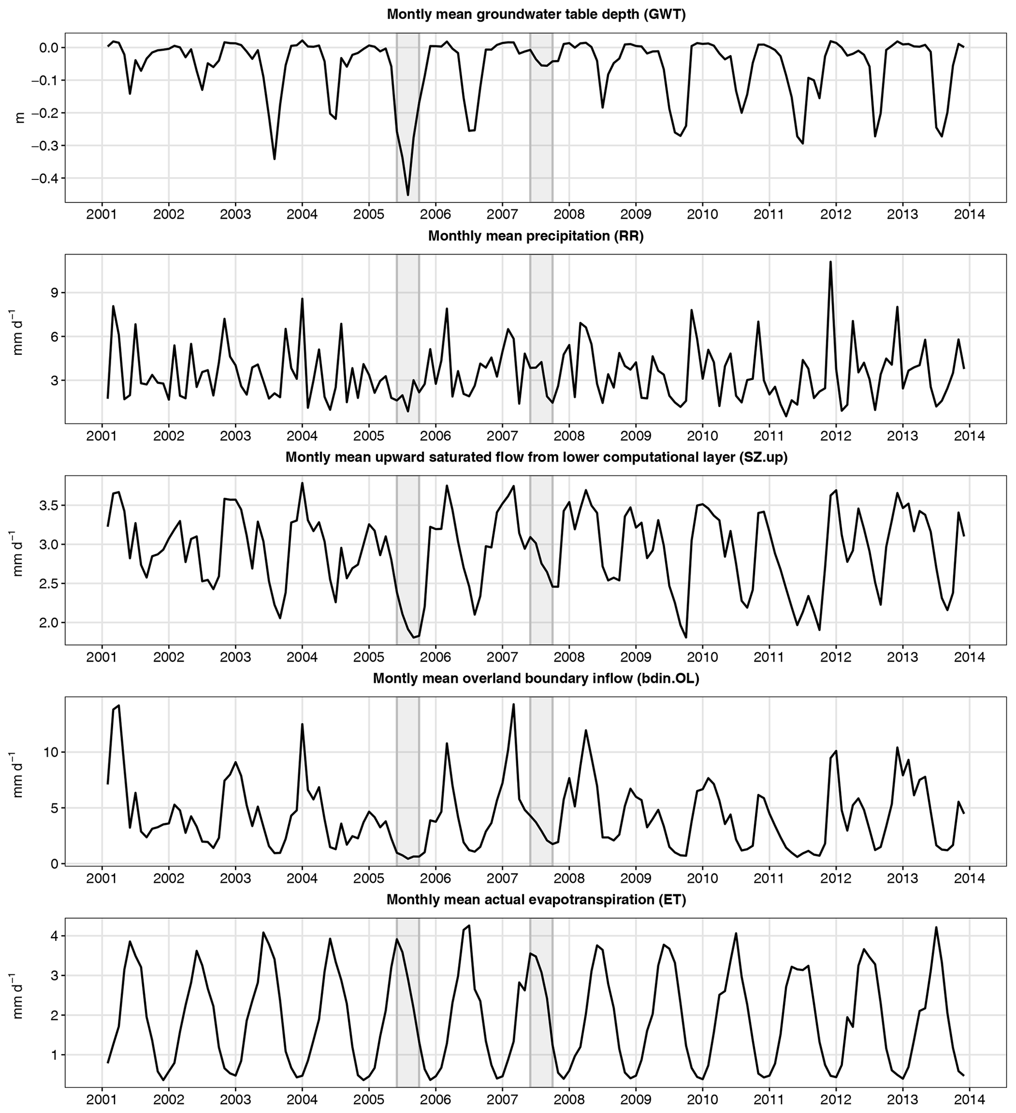
Figure 12Monthly means of simulated groundwater table depth and selected water balance items in the peat soil domain (2001–2013). Grey bands highlight two contrasting summers further described in Sect. 3.5.
Variation partitioning shows that, out of the four explanatory variables in the reduced model, groundwater upwelling explains the largest proportion of variation in groundwater table depth overall (70.3 %; see Fig. 14). However, due to collinearity, a large proportion of this variation is jointly explained by other variables, in particular groundwater table depth in the preceding month. Evapotranspiration explains 35.0 % of the variation in groundwater table depth, with 14.0 % of this being attributable to this variable independently of others.
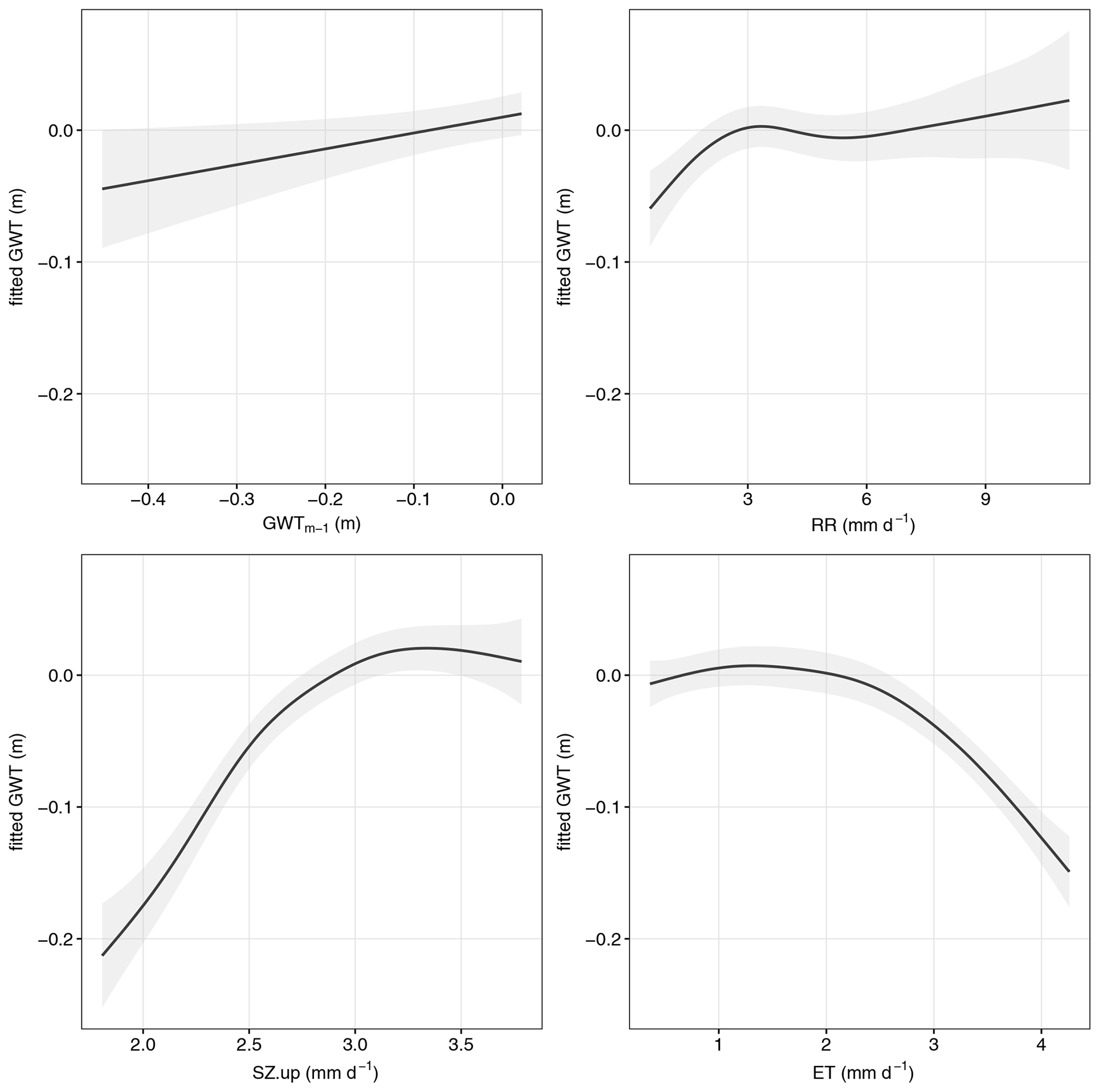
Figure 13Smooth terms of the final generalised additive model of simulated monthly mean groundwater table depth on the response scale. The curve shows the fitted value of the response, conditional upon the other explanatory variables being held at their sample mean. The shaded area is the approximate 95 % confidence interval. The time series used are simulated spatially averaged monthly means in the peat soil domain for the period 2001–2013: groundwater table depth (GWT), groundwater table depth in the preceding month (GWTm−1), upward saturated flow from the lower computational layer (SZ.up), actual evapotranspiration (ET) and precipitation (RR).

Figure 14Venn diagram of the variation partitioning results. The diagram shows the proportion of deviance in groundwater table depth (GWT) explained independently or jointly by groundwater table depth in the preceding month (GWTm−1), upward saturated flow from the lower computational layer (SZ.up), actual evapotranspiration (ET) and/or precipitation (RR), based on simulated spatially averaged monthly means in the peat soil domain for the period 2001–2013.
4.1 Modelling small granitic headwater catchments
Groundwater modelling in hard-rock regions is often described as difficult due to the heterogeneity of the substratum (e.g. Levison et al., 2014; Lubczynski and Gurwin, 2005; Neuman, 2005; Singhal and Gupta, 2010). In the Dauges catchment, poorer model performance in some locations (e.g. D4 and D5), an apparent trade-off between performance at dipwells located on three opposite margins of the mire (D3, D9, D10, D24 and D25), and detailed analysis of ERT results and geological drilling logs (Duranel, 2015) suggest that, at the very local scale, representation of the fissured zone as an homogenous entity may be an over-simplification. This is particularly the case for its hydraulic conductivity. The model was moderately sensitive to vertical saturated hydraulic conductivity of the fissured zone. Although the calibrated value was m s−1, values between and m s−1 produced similar results. The model was, however, highly sensitive to the horizontal hydraulic conductivity in the saturated fissured zone. This was the most important parameter controlling both stream discharge in the upper reaches and groundwater table in mineral and peat soils and the third most important parameter controlling discharge at the Pont de Pierre mire outlet. The calibrated value was m s−1. This is lower than the pumping test values reported by Dewandel et al. (2006) and Wyns et al. (2004), who suggested generic values of vertically and m s−1 horizontally, but very similar to values estimated through model calibration by Jaunat et al. (2016) in the Pyrenees (France), Ahmed and Sreedevi (2008) in India, Koïta et al. (2013) in Ivory Coast, and Hassan et al. (2014) in Spain. All of these authors, who worked on catchments significantly larger than the Dauges catchment, found that using spatially variable hydraulic conductivities for the weathered granite formations or introducing linear vertical barriers representing assumed or observed dykes, reefs or faults was necessary to achieve satisfactory performance. At the Dauges site, the ERT survey highlighted large variations in the electrical resistivity of the saturated fissured zone that are most probably related to variations in granite weathering, porosity and clay content. In particular, electrical resistivity was lower and the inferred degree of weathering higher at the bottom of the etch basin. This would agree with the current understanding of weathering and etching processes in granite landscapes (Godard et al., 2001). A homogeneous fissured layer is therefore clearly a simplification. Despite this, the model achieved satisfactory to very good overall performance with regard to groundwater table depths and discharge. In addition, there was very good agreement between the simulated long-term mean groundwater table depth and the observed distribution of mire habitats across the entire modelled area, including in places where no groundwater table depth observations were available for calibration. This demonstrates that, at least in some cases, saturated flow within weathered granite formations, including the fissured zone, can be reasonably well modelled at high spatial resolution using an equivalent porous medium approach and spatially homogeneous hydraulic parameters.
4.2 Modelling peatlands
In comparison to some long-term hydrological modelling studies of larger catchments, the hydrological time series assembled to calibrate and validate our model may appear relatively short. However, calibration and validation periods covering a total duration of 3 years (and often much less) are the norm rather than the exception in physically based hydrological modelling studies of wetlands (e.g. Ala-aho et al., 2017; Armandine Les Landes et al., 2014; Haahti et al., 2016; House et al., 2016a; Levison et al., 2014; Li et al., 2019; Quillet et al., 2017; Thompson et al., 2004). In many cases this is the result of the unfortunate exclusion of wetland environments from formal hydrometric networks (e.g. Hollis and Thompson, 1998) despite their ecological and socio-economic significance.
During calibration, the bed resistance of channels represented in MIKE 11 had to be increased substantially and beyond tabulated values given in the literature (Dingman, 1994) to improve performance with regard to discharge at the Pont de Pierre mire outlet. This reflects issues with the kinematic routing representation of discharge and stage within the mire. The low slope gradient, the shallow and ill-defined channel, the presence of shrubs and dense vegetation within the channel, and, in places, the subterranean course of the stream make the flow sluggish and create constant backwater effects. As a consequence, flooding and exchanges through highly permeable alluvial gravel deposits below the peat could not be accurately modelled, as evidenced by the poor performance for dipwells D8, D16 and D17. However, as shown by the good performance obtained for dipwells D18 and D19, the impact of the poor simulation of stream stage does not extend beyond the area where substantial alluvial deposits occur.
Mires are frequently characterised by a hummock and hollow micro-topography caused by peat accumulation and plant growth rates that vary at a very small spatial scale (Belyea and Clymo, 2001; Malmer et al., 1994). Purple moor-grass (Molinia caerulea) for instance can form tussocks that are up to 50 cm high. The definition of ground level is therefore a substantial methodological issue in mire hydrology (Whitfield et al., 2009), as this definition will have a profound impact on all quantities defined relative to ground level such as groundwater table depth or flood depth. Yet this definition is very rarely specified in most hydrological studies of mires. Van der Schaaf (2002) defined the surface level as “the average bottom level of the hollows within a radius of 1 m around a measuring point”. In the current study the surface level adjacent to groundwater monitoring instrumentation was taken as the mean of a minimum of three DGPS elevation measures taken within 30 cm of the dipwell and spread around it. In some dipwells this definition does not match the level at which overland flow starts to occur. This is the case for instance at dipwells D3, D7 and D12 where, except during the two or three driest months of the year, observed groundwater levels are constantly 3 to 6 cm above “ground level” when there is no substantial and permanent overland flow. This issue has a substantial and detrimental impact on model performance statistics but is difficult to resolve.
During model calibration, the peat specific yield and available water capacity had to be reduced substantially to 0.05 to reproduce observed groundwater table dynamics. These values are lower than those generally cited in the literature even for sapric peat. For example, based on a literature review, Letts et al. (2000) provided a mean value of 0.13 for the specific yield and 0.49 for the available water capacity of sapric peat. Specific yields similar to the value we obtained by calibration have, however, been reported elsewhere in degraded peatlands. Boelter (1968), Malloy and Price (2014) and Mustamo et al. (2016) measured specific yields of 0.08 in decomposed peats in northern Minnesota, circa 0.05 in a cut-over bog in Canada and 0.067 in a cultivated peatland in northern Finland, respectively. It is well known that peat physical properties are highly variable (Boelter, 1964, 1968; Brandyk et al., 2002; Gobat, 1990; Gobat et al., 1986; Grosvernier et al., 1999), and the lower specific yield produced by model calibration at the Dauges site may result from compaction by cattle or from a higher humification rate caused by drier climatic conditions encountered in central France compared to more northern latitudes where mires are more common and to which most of the available literature refers. The low calibrated value for available water capacity is more puzzling as it is an order of magnitude lower than those usually reported for peat soils (Letts et al., 2000). Very low values have sometimes been reported from degraded peat soils (Mustamo et al., 2016). It may also be an artefact of the two-layer unsaturated zone/evapotranspiration model, whereby the allowable range for soil moisture in the unsaturated zone has to be fully depleted before evapotranspiration can proceed from the saturated zone (DHI, 2009c) and impact groundwater levels. In wetlands where the groundwater level is usually within the root zone, representation of transpiration as a process drawing water from both unsaturated and saturated zones simultaneously might be more realistic.
Groundwater table depths within peat soils and discharge at the Pont de Pierre mire outlet were moderately sensitive to the saturated hydraulic conductivity of the peat layer. The calibrated value was almost identical to the median value obtained from slug tests in the catotelm ( m s−1 vs. ), implying low to moderate permeability and compatible with the high humification rate of the catotelm suggested by the calibrated specific yield and peat stratigraphic surveys. Slightly higher values (up to m s−1) gave relatively similar overall model performance but with a shift along the Pareto front towards better performance for discharge at the mire outlet and poorer performance for some dipwells. In particular, higher hydraulic conductivities led to slightly deeper groundwater table depths at the mire margins and shallower groundwater table depths at its centre. This suggests that the peat layer acts as an aquitard leading to the semi-confinement of the aquifer located in the underlying mineral formations, and to higher piezometric heads along the mire margins (see Rossi et al., 2012, for similar conclusions albeit in a different geological context). This process may have constituted a positive feedback to the mire's lateral expansion on steeper slopes and may have consequences for downstream discharge dynamics that should be further investigated.
4.3 Groundwater dependence of headwater mires in hard-rock regions
This study demonstrates that groundwater upwelling from underlying mineral formations can be a quantitatively important and functionally critical element of the water balance of valley mires in granitic headwater catchments. Runoff inputs to the Dauges mire (a substantial part of which actually originates from edge-focused groundwater seepage just upstream of the mire boundaries) are quantitatively slightly larger than precipitation and groundwater upwelling. However, both runoff and precipitation do not contribute substantially to the water balance of the peat layer since they quickly leave the mire as saturation-excess runoff due to the shallow water table. Water within the saturated peat overwhelmingly originates from groundwater upwelling from the underlying weathered granite formations. At the monthly timescale, groundwater upwelling explains the largest proportion of the variation in groundwater table depth within the mire. The influence of hydrological processes occurring in mineral formations upslope of the mire on the mire's water balance is further demonstrated by the much higher sensitivity of simulated groundwater levels in the peat to parameters describing hydrodynamic properties of weathered granite formations and mineral soils compared to those describing peat soils. It is very clear that there is a high degree of hydrological connectivity between weathered granite formations within the mire catchment and the mire itself.
There is a close match between spatial patterns of simulated groundwater upwelling and seepage and the observed distribution of mire habitats. Mire habitats seem to be particularly associated with areas where the long-term mean seepage rate in September is greater than zero. Good agreement between spatial patterns in wetland vegetation and groundwater upwelling and seepage has been reported for a number of wetlands that depend on large aquifers in sedimentary contexts (Faulkner et al., 2016; Gerla, 1999; Reeve and Gracz, 2008), but much more rarely in hard-rock regions without substantial sedimentary cover. As far as we are aware, the only study demonstrating this inter-relationship in a granitic context is that of Ala-aho et al. (2017). Using an integrated physics-based hydrological model of the 3.2 km2 Bruntland Burn catchment in Scotland, this previous study showed that valley bottom riparian peatlands coincided with steady groundwater upwelling and seepage which was responsible for persistent saturated conditions and overland flow generation even during dry periods. However, only the glacial drift sediments were considered to be hydrologically active, while the underlying granite bedrock was assumed to be impermeable. Drexler et al. (2013) showed that the areal extent of small mountainous fens in the Sierra Nevada (USA), located on a range of geological substrates including hard rocks, had decreased by between 10 % and 16 % over the last 50–80 years. They tentatively related these changes to a simultaneous increase in temperature and decrease in snowpack volume and longevity that together reduced groundwater recharge and, in turn, seepage to the fens. It was suggested that small mountainous fens might be used as whole-ecosystem gauges of groundwater recharge through time. The Dauges modelling study supports this assertion and changes in the factors impacting groundwater recharge within the mire catchment will likely impact spatial and temporal patterns of groundwater upwelling and seepage and, therefore, the distribution of mire vegetation. How quickly changes in groundwater upwelling rates would translate into modifications to mire vegetation is unknown. In contrast to mires dependant on large aquifers in sedimentary contexts, the hydrogeological catchments of headwater valley mires in hard-rock regions are likely to be relatively small in extent due to the relative shallowness of weathered formations compared to the surface relief. As a consequence, these mires are likely to be more sensitive to small-scale patterns and changes in groundwater recharge. As such, they may constitute useful whole catchment indicators to disentangle the respective impacts of local factors (changes in land use for instance) and regional factors (climate change in particular). This study only related spatial patterns in groundwater upwelling and seepage to the distribution of mire habitats as a whole. Future work could investigate in more detail whether groundwater upwelling and seepage rates are significant factors in explaining the variability in the species composition of headwater valley mires in hard-rock regions (Larocque et al., 2016; Munger et al., 2014).
The findings from this study have important management and legal implications. Indeed, the potential for anthropogenic pressures on groundwater bodies to indirectly impact groundwater-dependent terrestrial ecosystems (GWDTE) is now recognised in water resource legislation in many countries. In the European Union for instance, the Water Framework Directive (2000/60/EC) requires member states to ensure that water bodies, including groundwater bodies, achieve `good ecological status' which comprises a combination of good chemical and quantitative condition. Annex V of the Directive states that a groundwater body cannot achieve good status if the water table level is subject to anthropogenic alteration that would result in significant damage to terrestrial ecosystems that depend directly on the groundwater body. In practice the status of potential GWDTEs, in particular in hard-rock upland regions, is rarely or only superficially considered due to lack of understanding of the (i) impact of anthropogenic pressures on upland hard-rock aquifers; (ii) hydrological connectivity between hard-rock aquifers and terrestrial ecosystems; and (iii) hydrological controls on ecological conditions (Vernoux et al., 2010; Whiteman et al., 2010). Our study demonstrates that the Dauges mire depends directly on groundwater upwelling from the underlying mineral formations. Even though further work is required to upscale our conclusions, there is no reason to believe that the Dauges mire and its catchment are a unique case among valley mires in granitic headwaters. On the contrary, the Dauges site is representative of valley mires across the granitic Massif Central, and shares many similarities with other such systems found across the world, in particular throughout the Variscan Belt (Etlicher, 2005; Godard et al., 2001; Valadas, 1984, 1998). The results of this study show that the ecohydrological conditions of valley mires must be considered when assessing the status of hard-rock groundwater bodies under the Water Framework Directive.
In common with the Dauges mire, many headwater valley mires in hard-rock regions are designated for nature conservation under national or international legislation (Muller, 2018). Anthropogenic pressures on groundwater recharge within the catchments of these mires must be considered when defining conservation measures for these habitats or undertaking environmental impact assessments of policies and planning decisions. Article 6 of the EU 92/43/EEC Habitats Directive states that `any plan or project […] likely to have a significant effect thereon, either individually or in combination with other plans or projects, shall be subject to appropriate assessment of its implications for the site in view of the site's conservation objectives'. The present study demonstrates that any activities likely to result in substantial changes in groundwater flow within weathered granite formations upstream of the mire, even beyond SAC boundaries, do fall within the remit of this article. Examples of such activities include changes in land use such as large-scale afforestation and groundwater abstraction. Afforestation has, for example, been widespread within the Massif Central (Derrière et al., 2013; Dodane, 2009). The resulting changes in interception and evapotranspiration, with consequent impacts on surface and subsurface hydrological flow paths (Andréassian, 2004; Farley et al., 2005; Katzensteiner et al., 2011), may have had impacts on the region's mire ecosystems that should be further investigated.
Assuming that the relative importance of precipitation, runoff from mineral soil and groundwater seepage in the mire's overland component water balance reflects their relative contributions to overland inputs to water courses, 23 % of stream discharge at Pont de Pierre is water originating from the underlying mineral formations that has seeped through the peat layer. Excluding evapotranspiration, 46 % of water that flowed out of the saturated zone through seepage to overland flow, direct seepage to watercourses and groundwater flow out of the area upstream of Pont de Pierre did so through the peat layer. The vast majority (96 %) of the stream discharge at Pont de Pierre flowed at some point through the mire, either as overland flow or saturated flow. These figures highlight the importance of the mire as an interface between weathered granite formations and watercourses and hint at its potential role in mitigating the transfer of potential harmful compounds such as arsenic or uranium derived from the local geology (Mauroux et al., 2009) to water courses. Due to their organic soils and reductive conditions, pristine mires have been shown to constitute major sinks for almost all metallic and metalloid contaminants, and to efficiently reduce loads in downstream watercourses (Brown et al., 2000; González Acevedo et al., 2006; Lidman et al., 2012; Sobolewski, 1999). However, most of these studies have focussed on load reduction in watercourses as they flow through riparian mires, and further research is needed on load reduction in groundwater as it seeps through groundwater-fed mires.
Using an integrated MIKE SHE/MIKE 11 hydrological/hydraulic model, this study has shown that groundwater upwelling from weathered granite formations is a quantitatively important and functionally critical element of the water balance of the Dauges mire, a headwater valley mire in the granitic uplands of the French Massif Central. This is contrary to the “impermeable bedrock dogma” that has long been the dominant view in hard-rock hydrogeology and hillslope hydrology (Tromp-van Meerveld et al., 2007). Model performance in terms of simulated water table levels and stream discharge was at least satisfactory and in many locations good to very good. It included the replication of the seasonal rise and fall in groundwater levels. Based on model simulations, groundwater upwelling provided 27.1 % of total long-term inflows to the mire, rising to 37.2 % in September when total inflows are small. Furthermore, groundwater upwelling provided 92.4 % of total long-term inflows to the mire saturated zone. Variation partitioning showed that groundwater upwelling explained 70.3 % of the variation in monthly mean groundwater levels within the mire, although a large proportion of this is shared variation jointly explained by other variables, in particular groundwater table depth in the preceding month. The distribution of mire habitats within the catchment appears to be strongly controlled by groundwater upwelling. It was shown to closely coincide with areas where the simulated long-term mean groundwater seepage rate in September, the driest month associated with the lowest water table levels, is greater than zero. Model results demonstrate that the Dauges mire is a groundwater-dependent system closely connected to the granitic aquifer. This has important implications for the management and conservation of this and other similar ecosystems. However, whilst the Dauges mire is representative of acidic valley mires commonly found in many Variscan uplands, further work is required to upscale the conclusions of this study and to investigate how groundwater upwelling rates influence the ecology and biogeochemistry of such systems.
MIKE SHE/MIKE 11 is a commercial modelling software produced by DHI. Demo versions are available from http://www.mikepoweredbydhi.com/products/mike-she (DHI, 2021).
With the exception of secondary data derived under licence from third-party datasets, data used in this study are available upon reasonable request from the first author (arnaud.duranel@univ-st-etienne.fr). The meteorological data can be obtained from Météo-France.
The supplement related to this article is available online at: https://doi.org/10.5194/hess-25-291-2021-supplement.
AD designed and managed the study, installed the hydrometeorological network, collected all the data with the exception of manual checks, developed the geological conceptual model and MIKE SHE/MIKE 11 models, interpreted the results and wrote the first draft of the manuscript. JRT, HB and HC were AD's PhD supervisors and provided advice on the research design and on data analysis. JRT provided substantial expert advice on MIKE SHE/MIKE 11 and edited the initial manuscript. HC was principal investigator on the FEDER Loire and AELB grants that funded the hydrometeorological equipment and most field expenses. PD manages the Dauges National Nature Reserve. He contributed to the maintenance of the hydrometeorological network, completed regular manual checks, and provided substantial technical and logistical support during fieldwork. SG provided the ERT equipment, processed the ERT data and contributed to their interpretation. RW made a major contribution to the interpretation of the geological and geomorphological data and to the development of the geological model.
The authors declare that they have no conflict of interest.
The Conservatoire des Espaces Naturels de Nouvelle-Aquitaine and the Réserve Naturelle Nationale de la Tourbière des Dauges dedicated staff time to the collection of data used to develop the hydrological model. Météo-France provided part of the meteorological data. The Institut National de l'Information Géographique et Forestière, Areva (now Orano), the Conservatoire des Espaces Naturels de Nouvelle-Aquitaine and the Réserve Naturelle Nationale de la Tourbière des Dauges provided geological, topographic and cartographic data.
This research has been supported by a UK Natural Environmental Research Council doctoral studentship to Arnaud Duranel (grant no. NE/H525203/1) and a grant to UMR 5600 CNRS EVS from the European Fund for Regional Development (FEDER Loire) and the Agence de l'Eau Loire-Bretagne, obtained as part of the Plan Loire Grandeur Nature managed by the Établissement Public Loire (http://www.plan-loire.fr, last access: 12 January 2021) with additional contributions from the University of Saint-Etienne (project “Eco-hydrologie et fonctions des zones humides dans un contexte de changement climatique – L'exemple des têtes de bassin versant tourbeuses du Massif Central cristallin (Limousin et Monts du Forez)”).
This paper was edited by Philippe Ackerer and reviewed by two anonymous referees.
Ahmed, S. and Sreedevi, P. D.: Simulation of flow in weathered-fractured aquifer in a semi-arid and over-exploited region, in: Groundwater dynamics in hard rock aquifers: sustainable management and optimal monitoring network design, edited by: Ahmed, S., Jayakumar, R., and Salih, A., 219–233, Springer, Dordrecht, The Netherlands, 2008.
Ala-aho, P., Soulsby, C., Wang, H., and Tetzlaff, D.: Integrated surface-subsurface model to investigate the role of groundwater in headwater catchment runoff generation: A minimalist approach to parameterisation, J. Hydrol., 547, 664–677, https://doi.org/10.1016/j.jhydrol.2017.02.023, 2017.
Al-Khudhairy, D. H. A., Thompson, J. R., Gavin, H., and Hamm, N. A. S.: Hydrological modelling of a drained grazing marsh under agricultural land use and the simulation of restoration management scenarios, Hydrol. Sci. J., 44, 943–971, https://doi.org/10.1080/02626669909492291, 1999.
Allen, R. G. and Pereira, L. S.: Estimating crop coefficients from fraction of ground cover and height, Irrig. Sci., 28, 17–34, https://doi.org/10.1007/s00271-009-0182-z, 2009.
Allen, R. G., Pereira, L. S., Raes, D., and Smith, M.: Crop evapotranspiration – Guidelines for computing crop water requirements, FAO irrigation and drainage paper, Food and Agriculture Organization, Rome, Italy, 300 pp., 1998.
Andréassian, V.: Waters and forests: from historical controversy to scientific debate, J. Hydrol., 291, 1–27, https://doi.org/10.1016/j.jhydrol.2003.12.015, 2004.
Armandine Les Landes, A., Aquilina, L., De Ridder, J., Longuevergne, L., Pagé, C., and Goderniaux, P.: Investigating the respective impacts of groundwater exploitation and climate change on wetland extension over 150 years, J. Hydrol., 509, 367–378, https://doi.org/10.1016/j.jhydrol.2013.11.039, 2014.
Baize, D. and Girard, M.-C.: Référentiel pédologique 2008, Association française pour l'étude du sol, Editions Quae, Versailles, France, 2009.
Baker, C., Thompson, J. R., and Simpson, M.: Hydrological dynamics I: surface waters, flood and sediment dynamics, in: The Wetlands Handbook, edited by: Maltby, E. and Barker, T., Wiley-Blackwell, Chichester, UK, 120–168, 2009.
Baltassat, J. M., Legchenko, A., Ambroise, B., Mathieu, F., Lachassagne, P., Wyns, R., Mercier, J. L., and Schott, J. J.: Magnetic resonance sounding (MRS) and resistivity characterisation of a mountain hard rock aquifer: the Ringelbach Catchment, Vosges Massif, France, Surf. Geophys., 3, 267–274, https://doi.org/10.3997/1873-0604.2005022, 2005.
Banks, E. W., Simmons, C. T., Love, A. J., Cranswick, R., Werner, A. D., Bestland, E. A., Wood, M., and Wilson, T.: Fractured bedrock and saprolite hydrogeologic controls on groundwater/surface-water interaction: a conceptual model (Australia), Hydrogeol. J., 17, 1969–1989, https://doi.org/10.1007/s10040-009-0490-7, 2009.
Belyea, L. R. and Clymo, R. S.: Feedback control of the rate of peat formation, Proc. R. Soc. Lond. B Biol. Sci., 268, 1315–1321, https://doi.org/10.1098/rspb.2001.1665, 2001.
Boelter, D. H.: Water storage characteristics of several peats in situ, Soil Sci. Soc. Am. J., 28, 433–435, https://doi.org/10.2136/sssaj1964.03615995002800030039x, 1964.
Boelter, D. H.: Important physical properties of peat materials, in: Proceedings of the third international peat congress, Quebec, Canada, 18–23 August 1968, 150–154, 1968.
Boeye, D. and Verheyen, R. F.: The hydrological balance of a groundwater discharge fen, J. Hydrol., 137, 149–163, https://doi.org/10.1016/0022-1694(92)90053-X, 1992.
Bourgault, M. A., Larocque, M., and Roy, M.: Simulation of aquifer-peatland-river interactions under climate change, Hydrol. Res., 45, 425–440, https://doi.org/10.2166/nh.2013.228, 2014.
Brandyk, T., Szatylowicz, J., Oleszczuk, R., and Gnatowski, T.: Water-related physical attributes of organic soils, in: Organic soils and peat materials for sustainable agriculture, edited by: Parent, L. E. and Ilnicki, P., CRC Press, Boca Raton, FL, USA, 33–66, 2002.
Branfireun, B. A. and Roulet, N. T.: The baseflow and storm flow hydrology of a precambrian shield headwater peatland, Hydrol. Process., 12, 57–72, https://doi.org/10.1002/(SICI)1099-1085(199801)12:1<57::AID-HYP560>3.0.CO;2-U, 1998.
Brown, P. A., Gill, S. A., and Allen, S. J.: Metal removal from wastewater using peat, Water Res., 34, 3907–3916, https://doi.org/10.1016/S0043-1354(00)00152-4, 2000.
Brunner, P. and Simmons, C. T.: HydroGeoSphere: a fully integrated, physically based hydrological model, Ground Water, 50, 170–176, https://doi.org/10.1111/j.1745-6584.2011.00882.x, 2012.
Calder, I. R.: Assessing the water use of short vegetation and forests: development of the Hydrological Land Use Change (HYLUC) model, Water Resour. Res., 39, 1318, https://doi.org/10.1029/2003WR002040, 2003.
Clilverd, H. M., Thompson, J. R., Heppell, C. M., Sayer, C. D., and Axmacher, J. C.: Coupled hydrological/hydraulic modelling of river restoration impacts and floodplain hydrodynamics, River Res. Appl., 32, 1927–1948, https://doi.org/10.1002/rra.3036, 2016.
Commission of the European Communities: CORINE biotopes manual – A method to identify and describe consistently sites of major importance for nature conservation – Data specifications, Office for Official Publications of the European Communities, Luxembourg, 1991.
Congalton, R. G.: A review of assessing the accuracy of classifications of remotely sensed data, Remote Sens. Environ., 37, 35–46, https://doi.org/10.1016/0034-4257(91)90048-B, 1991.
Cubizolle, H.: Les tourbières et la tourbe, Lavoisier-Tec and Doc, Paris, France, 2019.
Delgado, J., Llorens, P., Nord, G., Calder, I. R., and Gallart, F.: Modelling the hydrological response of a Mediterranean medium-sized headwater basin subject to land cover change: The Cardener River basin (NE Spain), J. Hydrol., 383, 125–134, https://doi.org/10.1016/j.jhydrol.2009.07.024, 2010.
Derrière, N., Wurpillot, S., and Vidal, C.: Un siècle d'expansion des forêts françaises, De la statistique Daubrée à l'inventaire forestier de l'IGN, L'If, 31, 1–8, 2013.
Desire-Marchand, J. and Klein, C.: Le relief du Limousin. Les avatars d'un géomorphotype, Norois, 129, 23–49, https://doi.org/10.3406/noroi.1986.4292, 1986.
Dettmann, U. and Bechtold, M.: Deriving effective soil water retention characteristics from shallow water table fluctuations in peatlands, Vadose Zone J., 15, 1–13, https://doi.org/10.2136/vzj2016.04.0029, 2016.
Dewandel, B., Lachassagne, P., Wyns, R., Marechal, J. C., and Krishnamurthy, N. S.: A generalized 3-D geological and hydrogeological conceptual model of granite aquifers controlled by single or multiphase weathering, J. Hydrol., 330, 260–284, https://doi.org/10.1016/j.jhydrol.2006.03.026, 2006.
DHI: AUTOCAL – Auto calibration tool user guide, DHI, Hørsholm, Denmark, 2009a.
DHI: MIKE 11 – A modelling system for rivers and channels, Reference manual, DHI, Hørsholm, Denmark, 2009b.
DHI: MIKE SHE user manual, Volume 2, Reference guide, DHI, Hørsholm, Denmark, 2009c.
DHI: MIKE SHE, commercial modelling software, available at: http://www.mikepoweredbydhi.com/products/mike-she, last access: 12 January 2021.
Dingman, S. L.: Physical hydrology, Macmillan Publishing Company, New York, USA, 1994.
Dodane, C.: Les nouvelles forêts du Massif Central : enjeux sociétaux et territoriaux. Ces hommes qui plantaient des résineux pour éviter la friche, PhD thesis, Ecole normale supérieure Lettres et Sciences Humaines Lyon, Lyon, France, available at: https://tel.archives-ouvertes.fr/tel-00466263/document (last access: 6 March 2015), 2009.
Drexler, J. Z., Knifong, D., Tuil, J., Flint, L. E., and Flint, A. L.: Fens as whole-ecosystem gauges of groundwater recharge under climate change, J. Hydrol., 481, 22–34, https://doi.org/10.1016/j.jhydrol.2012.11.056, 2013.
Duranel, A. J.: Hydrology and hydrological modelling of acidic mires in central France, PhD thesis, University College London, London, UK, available at: http://discovery.ucl.ac.uk/1472054/1/Duranel_PhDthesisADuranel2015.pdf (last access: 12 January 2021), 2015.
Durepaire, P. and Guerbaa, K.: Tourbière des Dauges – Plan de gestion 2008–2012, Conservatoire Régional des Espaces Naturels du Limousin, St-Gence, France, 2008.
Etlicher, B.: French and Belgian Uplands, in: The physical geography of Western Europe, vol. 6, edited by: Koster, E. A., Oxford University Press, Oxford, UK, 231–250, 2005.
Farley, K. A., Jobbágy, E. G., and Jackson, R. B.: Effects of afforestation on water yield: a global synthesis with implications for policy, Glob. Change Biol., 11, 1565–1576, https://doi.org/10.1111/j.1365-2486.2005.01011.x, 2005.
Faulkner, B. R., Leibowitz, S. G., Canfield, T. J., and Groves, J. F.: Quantifying groundwater dependency of riparian surface hydrologic features using the exit gradient, Hydrol. Process., 30, 2167–2177, https://doi.org/10.1002/hyp.10766, 2016.
Frolking, S., Talbot, J., Jones, M. C., Treat, C. C., Kauffman, J. B., Tuittila, E.-S., and Roulet, N.: Peatlands in the Earth's 21st century climate system, Environ. Rev., 19, 371–396, https://doi.org/10.1139/a11-014, 2011.
Gabrielli, C. P., McDonnell, J. J., and Jarvis, W. T.: The role of bedrock groundwater in rainfall-runoff response at hillslope and catchment scales, J. Hydrol., 450/451, 117–133, https://doi.org/10.1016/j.jhydrol.2012.05.023, 2012.
Gerla, P.: Estimating the ground-water contribution in wetlands using modeling and digital terrain analysis, Wetlands, 19, 394–402, https://doi.org/10.1007/BF03161771, 1999.
Gilvear, D. J. and Bradley, C.: Hydrological dynamics II: groundwater and hydrological connectivity, in: The Wetlands Handbook, edited by: Maltby, E. and Barker, T., Wiley-Blackwell, Chichester, UK, 169–193, 2009.
Gilvear, D. J., Andrews, R., Tellam, J. H., Lloyd, J. W., and Lerner, D. N.: Quantification of the water balance and hydrogeological processes in the vicinity of a small groundwater-fed wetland, East Anglia, UK, J. Hydrol., 144, 311–334, https://doi.org/10.1016/0022-1694(93)90178-C, 1993.
Gobat, J. M.: Quelques relations entre la végétation et la qualité physico-chimique des tourbes dans le Jura, Bull. Société Neuchâtel. Sci. Nat., 113, 207–214, 1990.
Gobat, J. M., Grosvernier, P., and Matthey, Y.: Les tourbières du Jura suisse: milieux naturels, modifications humaines, caractères des tourbes, potentiel de régénération, Actes Société Jurassienne Emulation, 89, 213–318, 1986.
Godard, A., Lagasquie, J. J., and Lageat, Y.: Basement Regions, Springer-Verlag, Berlin and Heidelberg, Germany, 2001.
González Acevedo, Z. I., Krachler, M., Cheburkin, A. K., and Shotyk, W.: Spatial distribution of natural enrichments of arsenic, selenium, and uranium in a minerotrophic peatland, Gola di Lago, Canton Ticino, Switzerland, Environ. Sci. Technol., 40, 6568–6574, https://doi.org/10.1021/es061080v, 2006.
Graham, D. N. and Butts, M. B.: Flexible, integrated watershed modelling with MIKE SHE, in: Watershed models, edited by: Singh, V. P. and Frevert, D. K., CRC Press, Boca Raton, Florida, USA, 245–272, 2005.
Grosvernier, P. R., Matthey, Y., Buttler, A., and Gobat, J. M.: Characterization of peats from histosols disturbed by different human impacts (drainage, peat extraction, agriculture), Ecologie, 30, 23–31, 1999.
Guihéneuf, N., Boisson, A., Bour, O., Dewandel, B., Perrin, J., Dausse, A., Viossanges, M., Chandra, S., Ahmed, S., and Maréchal, J. C.: Groundwater flows in weathered crystalline rocks: Impact of piezometric variations and depth-dependent fracture connectivity, J. Hydrol., 511, 320–334, https://doi.org/10.1016/j.jhydrol.2014.01.061, 2014.
Haahti, K., Warsta, L., Kokkonen, T., Younis, B. A., and Koivusalo, H.: Distributed hydrological modeling with channel network flow of a forestry drained peatland site, Water Resour. Res., 52, 246–263, https://doi.org/10.1002/2015WR018038, 2016.
Hammersmark, C. T., Dobrowski, S. Z., Rains, M. C., and Mount, J. F.: Simulated effects of stream restoration on the distribution of wet-meadow vegetation, Restor. Ecol., 18, 882–893, https://doi.org/10.1111/j.1526-100X.2009.00519.x, 2010.
Haria, A. H. and Shand, P.: Evidence for deep sub-surface flow routing in forested upland Wales: implications for contaminant transport and stream flow generation, Hydrol. Earth Syst. Sci., 8, 334–344, https://doi.org/10.5194/hess-8-334-2004, 2004.
Hassan, S. M. T., Lubczynski, M. W., Niswonger, R. G., and Su, Z.: Surface-groundwater interactions in hard rocks in Sardon Catchment of western Spain: An integrated modeling approach, J. Hydrol., 517, 390–410, https://doi.org/10.1016/j.jhydrol.2014.05.026, 2014.
Hollis, G. E. and Thompson, J. R.: Hydrological data for wetland management, Water Environ. J., 12, 9–17, https://doi.org/10.1111/j.1747-6593.1998.tb00140.x, 1998.
House, A. R., Thompson, J. R., Sorensen, J. P. R., Roberts, C., and Acreman, M. C.: Modelling groundwater/surface water interaction in a managed riparian chalk valley wetland, Hydrol. Process., 30, 447–462, https://doi.org/10.1002/hyp.10625, 2016a.
House, A. R., Thompson, J. R., and Acreman, M. C.: Projecting impacts of climate change on hydrological conditions and biotic responses in a chalk valley riparian wetland, J. Hydrol., 534, 178–192, https://doi.org/10.1016/j.jhydrol.2016.01.004, 2016b.
Ingram, H. A. P.: Soil layers in mires: function and terminology, J. Soil Sci., 29, 224–227, https://doi.org/10.1111/j.1365-2389.1978.tb02053.x, 1978.
Ivanov, K. E.: Gidrologiya bolot, Gidrometeoizdat, Leningrad, Russia, 1953.
Jaunat, J., Dupuy, A., Huneau, F., Celle-Jeanton, H., and Coustumer, P. L.: Groundwater flow dynamics of weathered hard-rock aquifers under climate-change conditions: an illustrative example of numerical modeling through the equivalent porous media approach in the north-western Pyrenees (France), Hydrogeol. J., 24, 1359–1373, https://doi.org/10.1007/s10040-016-1408-9, 2016.
Joly, D., Brossard, T., Cardot, H., Cavailhes, J., Hilal, M., and Wavresky, P.: Les types de climats en France, une construction spatiale, Cybergeo Eur. J. Geogr., 501, 23155, https://doi.org/10.4000/cybergeo.23155, 2010.
Katzensteiner, K., Klimo, E., Szuckics, U., and Delaney, C. M.: Impact of forest management alternatives on water budgets and runoff processes, in: Papers on impacts of forest management on environmental services, edited by: Raulund-Rasmussen, K., De Jong, J., Humphrey, J. W., Smith, M., Ravn, H. P., Katzensteiner, K., Klimo, E., Szuckics, U., Delaney, C. M., Hansen, K., Stupak, I., Ring, E., Gundersen, P., and Lousteau, D., European Forest Institute, Joensuu, Finland, 27–55, 2011.
Klein, C.: Les Monts d'Ambazac et de Saint-Goussaud. Deux points de vue sur la morphogenèse limousine, Norois, 97, 103–126, https://doi.org/10.3406/noroi.1978.3679, 1978.
Klein, C., Désiré-Marchand, J., and Giusti, C.: L'évolution géomorphologique de l'Europe hercynienne occidentale et centrale: aspects régionaux et essai de synthèse, Centre National de la Recherche Scientifique, Paris, France, 1990.
Koerselman, W.: Groundwater and surface water hydrology of a small groundwater-fed fen, Wetl. Ecol. Manag., 1, 31–43, https://doi.org/10.1007/BF00177888, 1989.
Koïta, M., Jourde, H., and Rossier, Y.: Relative importance of weathering profiles and major fracture zones to fit the water balance of a hydrogeological catchment in hard rocks, Int. J. Environ. Sci., 4, 296, available at: http://www.indianjournals.com/ijor.aspx?target=ijor:ijes&volume=4&issue=3&article=008 (last access: 12 January 2021), 2013.
Kosugi, K., Katsura, S., Katsuyama, M., and Mizuyama, T.: Water flow processes in weathered granitic bedrock and their effects on runoff generation in a small headwater catchment, Water Resour. Res., 42, W02414, https://doi.org/10.1029/2005WR004275, 2006.
Kosugi, K., Fujimoto, M., Katsura, S., Kato, H., Sando, Y., and Mizuyama, T.: Localized bedrock aquifer distribution explains discharge from a headwater catchment, Water Resour. Res., 47, W07530, https://doi.org/10.1029/2010WR009884, 2011.
Lachassagne, P.: Overview of the hydrogeology of hard rock aquifers: applications for their survey, management, modelling and protection, in: Groundwater dynamics in hard rock aquifers: sustainable management and optimal monitoring network design, edited by: Ahmed, S., Jayakumar, R., and Salih, A., Springer, Dordrecht, The Netherlands, 40–63, 2008.
Lachassagne, P., Wyns, R., and Dewandel, B.: The fracture permeability of hard rock aquifers is due neither to tectonics, nor to unloading, but to weathering processes, Terra Nova, 23, 145–161, https://doi.org/10.1111/j.1365-3121.2011.00998.x, 2011.
Larocque, M., Ferlatte, M., Pellerin, S., Cloutier, V., Munger, J. L., Paniconi, C., and Quillet, A.: Chemical and botanical indicators of groundwater inflow to Sphagnum-dominated peatlands, Ecol. Indic., 64, 142–151, https://doi.org/10.1016/j.ecolind.2015.12.012, 2016.
Legendre, P. and Legendre, L.: Numerical ecology, 2nd ed., Elsevier Science, Amsterdam, The Netherlands, 1998.
Letts, M. G., Roulet, N. T., Comer, N. T., Skarupa, M. R., and Verseghy, D. L.: Parametrization of peatland hydraulic properties for the Canadian Land Surface Scheme, Atmosphere-Ocean, 38, 141–160, https://doi.org/10.1080/07055900.2000.9649643, 2000.
Levison, J., Larocque, M., Fournier, V., Gagné, S., Pellerin, S., and Ouellet, M. A.: Dynamics of a headwater system and peatland under current conditions and with climate change, Hydrol. Process., 28, 4808–4822, https://doi.org/10.1002/hyp.9978, 2014.
Li, Z., Gao, P., and Lu, H.: Dynamic changes of groundwater storage and flows in a disturbed alpine peatland under variable climatic conditions, J. Hydrol., 575, 557–568, https://doi.org/10.1016/j.jhydrol.2019.05.032, 2019.
Lidman, F., Mörth, C. M., and Laudon, H.: Landscape control of uranium and thorium in boreal streams – spatiotemporal variability and the role of wetlands, Biogeosciences, 9, 4773–4785, https://doi.org/10.5194/bg-9-4773-2012, 2012.
Lindsay, R.: Peatbogs and carbon: a critical synthesis to inform policy development in oceanic peat bog conservation and restoration in the context of climate change, Environmental Research Group, University of East London, London, UK, 2010.
Loke, M. H.: RES2DINVx32/x64 – 2D resistivity and IP inversion software for Windows XP/Vista/7, Geotomo Software SDN BHD, Gelugor, Malaysia, 2013.
Loke, M. H. and Barker, R. D.: Rapid least-squares inversion of apparent resistivity pseudosections by a quasi-Newton method, Geophys. Prospect., 44, 131–152, https://doi.org/10.1111/j.1365-2478.1996.tb00142.x, 1996.
Long, J. C. S., Remer, J. S., Wilson, C. R., and Witherspoon, P. A.: Porous media equivalents for networks of discontinuous fractures, Water Resour. Res., 18, 645–658, https://doi.org/10.1029/WR018i003p00645, 1982.
Lubczynski, M. W. and Gurwin, J.: Integration of various data sources for transient groundwater modeling with spatio-temporally variable fluxes – Sardon study case, Spain, J. Hydrol., 306, 71–96, https://doi.org/10.1016/j.jhydrol.2004.08.038, 2005.
Malloy, S. and Price, J. S.: Fen restoration on a bog harvested down to sedge peat: A hydrological assessment, Ecol. Eng., 64, 151–160, https://doi.org/10.1016/j.ecoleng.2013.12.015, 2014.
Malmer, N., Svensson, B. M., and Wallén, B.: Interactions between Sphagnum mosses and field layer vascular plants in the development of peat-forming systems, Folia Geobot., 29, 483–496, https://doi.org/10.1007/BF02883146, 1994.
Maréchal, J. C., Wyns, R., Lachassagne, P., and Subrahmanyam, K.: Vertical anisotropy of hydraulic conductivity in the fissured layer of hard-rock aquifers due to the geological structure of weathering profiles, J. Geol. Soc. India, 63, 545–550, 2004.
Mauroux, B., Wyns, R., Martelet, G., and Lions, J.: SILURES Limousin – Module 1 SILURES “Base de données”. Recueil des données, interprétations et perspectives, Rapport final, Bureau de Recherches Géologiques et Minières, Orléans, France, 2009.
Moriasi, D. N., Arnold, J. G., Van Liew, M. W., Bingner, R. L., Harmel, R. D., and Veith, T. L.: Model evaluation guidelines for systematic quantification of accuracy in watershed simulations, Trans. Am. Soc. Agric. Biol. Eng., 50, 885–900, https://doi.org/10.13031/2013.23153, 2007.
Morley, T. R., Reeve, A. S., and Calhoun, A. J. K.: The role of headwater wetlands in altering streamflow and chemistry in a Maine, USA catchment, JAWRA J. Am. Water Resour. Assoc., 47, 337–349, https://doi.org/10.1111/j.1752-1688.2010.00519.x, 2011.
Muller, F.: Strategies for peatland conservation in France – a review of progress, Mires Peat, 21, 1–13, https://doi.org/10.19189/MaP.2016.OMB.218, 2018.
Munger, J. L., Pellerin, S., Larocque, M., and Ferlatte, M.: Espèces végétales indicatrices des échanges d'eau entre tourbière et aquifère, Nat. Can., 138, 4–12, https://doi.org/10.7202/1021038ar, 2014.
Mustamo, P., Hyvärinen, M., Ronkanen, A.-K., and Kløve, B.: Physical properties of peat soils under different land use options, Soil Use Manag., 32, 400–410, https://doi.org/10.1111/sum.12272, 2016.
Neuman, S. P.: Trends, prospects and challenges in quantifying flow and transport through fractured rocks, Hydrogeol. J., 13, 124–147, https://doi.org/10.1007/s10040-004-0397-2, 2005.
Okruszko, T., Duel, H., Acreman, M., Grygoruk, M., Flörke, M., and Schneider, C.: Broad-scale ecosystem services of European wetlands – overview of the current situation and future perspectives under different climate and water management scenarios, Hydrol. Sci. J., 56, 1501–1517, https://doi.org/10.1080/02626667.2011.631188, 2011.
Parish, F., Sirin, A., Charman, D., Joosten, H., Minayeva, T., Silvius, M., and Stringer, L.: Assessment on peatlands, biodiversity and climate change, Main report, Global Environment Centre and Wetlands International, Kuala Lumpur, Malaysia and Wageningen, The Netherlands, 2008.
Quillet, A., Larocque, M., Pellerin, S., Cloutier, V., Ferlatte, M., Paniconi, C., and Bourgault, M.-A.: The role of hydrogeological setting in two Canadian peatlands investigated through 2D steady-state groundwater flow modelling, Hydrol. Sci. J., 62, 2541–2557, https://doi.org/10.1080/02626667.2017.1391387, 2017.
Reeve, A. S. and Gracz, M.: Simulating the hydrogeologic setting of peatlands in the Kenai Peninsula Lowlands, Alaska, Wetlands, 28, 92–106, https://doi.org/10.1672/07-71.1, 2008.
Refsgaard, J. C., Storm, B., and Clausen, T.: Système Hydrologique Europeén (SHE): review and perspectives after 30 years development in distributed physically-based hydrological modelling, Hydrol. Res., 41, 355, https://doi.org/10.2166/nh.2010.009, 2010.
Richardson, J. L., Arndt, J. L., and Montgomery, J. A.: Hydrology of wetland and related soils, in: Wetland soils – Genesis, hydrology, landscapes, and classification, edited by: Richardson, J. L. and Vepraskas, M. J., CRC Press, Boca Raton, FL, USA, 35–84, 2001.
Rochester, R. E. L.: Uncertainty in hydrological modelling: a case study in the Tern catchment, Shropshire, UK, PhD thesis, University College London, London, UK, available at: http://discovery.ucl.ac.uk/795428/ (last access: 24 November 2011), 2010.
Romanov, V. V.: Hydrophysics of Bogs [Gidrofizika bolot (1961)], edited by: Heimann, A., Israel Program for Scientific Translation, Jerusalem, Israel, 1968.
Rossi, P. M., Ala-aho, P., Ronkanen, A.-K., and Kløve, B.: Groundwater-surface water interaction between an esker aquifer and a drained fen, J. Hydrol., 432/433, 52–60, https://doi.org/10.1016/j.jhydrol.2012.02.026, 2012.
Rydin, H. and Jeglum, J. K.: The biology of peatlands, Oxford University Press, Oxford, UK, 2006.
Šanda, M., Vitvar, T., Kulasová, A., Jankovec, J., and Císlerová, M.: Run-off formation in a humid, temperate headwater catchment using a combined hydrological, hydrochemical and isotopic approach (Jizera Mountains, Czech Republic), Hydrol. Process., 28, 3217–3229, https://doi.org/10.1002/hyp.9847, 2014.
Siegel, D. I. and Glaser, P. H.: Groundwater flow in a bog-fen complex, Lost River peatland, northern Minnesota, J. Ecol., 75, 743–754, https://doi.org/10.2307/2260203, 1987.
Singhal, B. B. S. and Gupta, R. P.: Applied hydrogeology of fractured rocks, 2nd ed., Springer, Dordrecht, The Netherlands, 2010.
Sobolewski, A.: A review of processes responsible for metal removal in wetlands treating contaminated mine drainage, Int. J. Phytoremediation, 1, 19–51, https://doi.org/10.1080/15226519908500003, 1999.
Tanneberger, F., Tegetmeyer, C., Busse, S., Barthelmes, A., Shumka, S., Moles, M., Jenderedjian, K., Steiner, G. M., Essl, F., Etzold, J., Mendes, C., Kozulin, A., Frankard, P., Milanović, D. J., Ganeva, A., Apostolova, I., Alegro, A., Delipetrou, P., Navrátilová, J., Risager, M., Leivits, A., Fosaa, A. M., Tuominen, S., Muller, F., Bakuradze, T., Sommer, M., Christanis, K., Szurdoki, E., Oskarsson, H., Brink, S. H., Connolly, J., Bragazza, L., Martinelli, G., Aleksāns, O., Priede, A., Sungaila, D., Melovski, L., Belous, T., Saveljić, D., de Vries, F., Moen, A., Dembek, W., Mateus, J., Hanganu, J., Sirin, A., Markina, A., Napreenko, M., Lazarević, P., Šefferová Stanová, V., Skoberne, P., Heras Pérez, P., Pontevedra-Pombal, X., Lonnstad, J., Küchler, M., Wüst-Galley, C., Kirca, S., Mykytiuk, O., Lindsay, R., and Joosten, H.: The peatland map of Europe, Mires Peat, 19, 1–17, https://doi.org/10.19189/MaP.2016.OMB.264, 2017.
Thompson, J., Gavin, H., Refsgaard, A., Refstrup Sørenson, H., and Gowing, D.: Modelling the hydrological impacts of climate change on UK lowland wet grassland, Wetl. Ecol. Manag., 17, 503–523, https://doi.org/10.1007/s11273-008-9127-1, 2009.
Thompson, J. R.: Simulation of wetland water-level manipulation using coupled hydrological/hydraulic modeling, Phys. Geogr., 25, 39–67, https://doi.org/10.2747/0272-3646.25.1.39, 2004.
Thompson, J. R.: Modelling the impacts of climate change on upland catchments in southwest Scotland using MIKE SHE and the UKCP09 probabilistic projections, Hydrol. Res., 43, 507, https://doi.org/10.2166/nh.2012.105, 2012.
Thompson, J. R., Sørenson, H. R., Gavin, H., and Refsgaard, A.: Application of the coupled MIKE SHE/MIKE 11 modelling system to a lowland wet grassland in southeast England, J. Hydrol., 293, 151–179, https://doi.org/10.1016/j.jhydrol.2004.01.017, 2004.
Thompson, J. R., Iravani, H., Clilverd, H. M., Sayer, C. D., Heppell, C. M., and Axmacher, J. C.: Simulation of the hydrological impacts of climate change on a restored floodplain, Hydrol. Sci. J., 62, 2482–2510, https://doi.org/10.1080/02626667.2017.1390316, 2017.
Tromp-van Meerveld, H. J., Peters, N. E., and McDonnell, J. J.: Effect of bedrock permeability on subsurface stormflow and the water balance of a trenched hillslope at the Panola Mountain Research Watershed, Georgia, USA, Hydrol. Process., 21, 750–769, https://doi.org/10.1002/hyp.6265, 2007.
Uchida, T., Asano, Y., Ohte, N., and Mizuyama, T.: Seepage area and rate of bedrock groundwater discharge at a granitic unchanneled hillslope, Water Resour. Res., 39, 1018, https://doi.org/10.1029/2002WR001298, 2003.
Valadas, B.: Les hautes terres du Massif Central français: contribution à l'étude des morphodynamiques récentes sur versants cristallins et volcaniques, PhD thesis, Université Paris I, Paris, France, 1984.
Valadas, B.: L'alvéole des Dauges : un modèle géomorphologique, Ann. Sci. Limousin, N∘ spécial: Tourbière des Dauges, 5–13, https://doi.org/10.25965/asl.913, 1998.
van der Schaaf, S.: Analysis of the hydrology of raised bogs in the Irish Midlands. A case study of Raheenmore bog and Clara bog, PhD thesis, Wageningen Agricultural University, Wageningen, The Netherlands, 1999.
van der Schaaf, S.: Bog hydrology, in: Conservation and restoration of raised bogs: geological, hydrological and ecological studies, edited by: Schouten, M. G. C., Stationery Office, Dublin, Ireland, 54–109, 2002.
Verger, J. P.: Les sols de l'alvéole de la tourbière du ruisseau des Dauges (Limousin), Ann. Sci. Limousin, N∘ spécial : Tourbière des Dauges, 43–54, https://doi.org//10.25965/asl.929, 1998.
Vernoux, J. F., Llons, J., Petelet-Giraud, E., Seguin, J. J., and Stollsteiner, P.: Contribution à la caractérisation des relations entre eau souterraine, eau de surface et écosystèmes terrestres associés en lien avec la DCE, Rapport final, Bureau de Recherches Géologiques et Minières, Orléans, France, 2010.
Wassen, M. J., Barendregt, A., Schot, P. P., and Beltman, B.: Dependency of local mesotrophic fens on a regional groundwater flow system in a poldered river plain in the Netherlands, Landsc. Ecol., 5, 21–38, https://doi.org/10.1007/BF00153801, 1990.
Wheeler, B. D., Gowing, D. J. G., Shaw, S. C., Mountford, J. O., and Money, R. P.: Ecohydrological guidelines for lowland wetland plant communities, Environment Agency (Anglian Region), Peterborough, UK, 2004.
Whiteman, M., Brooks, A., Skinner, A., and Hulme, P.: Determining significant damage to groundwater-dependent terrestrial ecosystems in England and Wales for use in implementation of the Water Framework Directive, Ecol. Eng., 36, 1118–1125, https://doi.org/10.1016/j.ecoleng.2010.03.013, 2010.
Whitfield, P. H., St-Hilaire, A., and van der Kamp, G.: Improving hydrological predictions in peatlands, Can. Water Resour. J., 34, 467–478, https://doi.org/10.4296/cwrj3404467, 2009.
Wood, S.: Package “mgcv”. Mixed GAM computation vehicle with automatic smoothness estimation, available at: http://cran.r-project.org/web/packages/mgcv (last access: 12 January 2021), 2016.
Worrall, F., Chapman, P., Holden, J., Evans, C., Artz, R., Smith, P., and Grayson, R.: A review of current evidence on carbon fluxes and greenhouse gas emissions from UK peatlands, JNCC report, Joint Nature Conservation Committee, Peterborough, UK, 2011.
Wyns, R., Baltassat, J.-M., Lachassagne, P., Legchenko, A., Vairon, J., and Mathieu, F.: Application of proton magnetic resonance soundings to groundwater reserve mapping in weathered basement rocks (Brittany, France), Bull. Société Géologique Fr., 175, 21–34, https://doi.org/10.2113/175.1.21, 2004.
Yan, J. and Smith, K. R.: Simulation of integrated surface water and ground water systems-model formulation, J. Am. Water Resour. Assoc., 30, 879–890, https://doi.org/10.1111/j.1752-1688.1994.tb03336.x, 1994.
Yu, Z., Beilman, D. W., Frolking, S., MacDonald, G. M., Roulet, N. T., Camill, P., and Charman, D. J.: Peatlands and their role in the global carbon cycle, Eos Trans. Am. Geophys. Union, 92, 97–98, https://doi.org/10.1029/2011EO120001, 2011.