the Creative Commons Attribution 4.0 License.
the Creative Commons Attribution 4.0 License.
 | 19 May 2021
GRAINet: mapping grain size distributions in river beds from UAV images with convolutional neural networks
Andrea Irniger
Agnieszka Rozniak
Roni Hunziker
Jan Dirk Wegner
Konrad Schindler
Grain size analysis is the key to understand the sediment dynamics of river systems. We propose GRAINet, a data-driven approach to analyze grain size distributions of entire gravel bars based on georeferenced UAV images. A convolutional neural network is trained to regress grain size distributions as well as the characteristic mean diameter from raw images. GRAINet allows for the holistic analysis of entire gravel bars, resulting in (i) high-resolution estimates and maps of the spatial grain size distribution at large scale and (ii) robust grading curves for entire gravel bars. To collect an extensive training dataset of 1491 samples, we introduce digital line sampling as a new annotation strategy. Our evaluation on 25 gravel bars along six different rivers in Switzerland yields high accuracy: the resulting maps of mean diameters have a mean absolute error (MAE) of 1.1 cm, with no bias. Robust grading curves for entire gravel bars can be extracted if representative training data are available. At the gravel bar level the MAE of the predicted mean diameter is even reduced to 0.3 cm, for bars with mean diameters ranging from 1.3 to 29.3 cm. Extensive experiments were carried out to study the quality of the digital line samples, the generalization capability of GRAINet to new locations, the model performance with respect to human labeling noise, the limitations of the current model, and the potential of GRAINet to analyze images with low resolutions.
- Article
(21743 KB) - Full-text XML
- BibTeX
- EndNote


Understanding the hydrological and geomorphological processes of rivers is crucial for their sustainable development so as to mitigate the risk of extreme flood events and to preserve the biodiversity in aquatic habitats. Grain size data of gravel- and cobble-bed streams are key to advance the understanding and modeling of such processes (Bunte and Abt, 2001). The fluvial morphology of the majority of the world's streams is heavily affected by human activity and construction along the river (Grill et al., 2019). Human interventions like gravel extractions, sediment retention basins in the upper catchments, hydroelectric power plants, dams, or channels reduce the bed load and lead to surface armoring, clogging of the bed, and latent erosion (Surian and Rinaldi, 2003; Simon and Rinaldi, 2006; Poeppl et al., 2017; Gregory, 2019). Consequently, the natural alteration of the river bed is hindered, eventually deteriorating habitats and potential spawning grounds. Moreover, the process of bed-load transport can cause bed or bank erosion, the destruction of engineering structures (e.g., due to bridge scours), or increased flooding due to deposits in the channel that amplify the impact of severe floods (Badoux et al., 2014). What makes modeling of fluvial morphology challenging are the mutual dependencies between the flow field, grain size, movement, and geometry of the channel bed and banks. While channel shape and roughness define the flow field, the flow moves sediments – depending on their size – and the bed is altered by erosion and deposition. This mutually reinforcing system makes understanding channel form and processes hard. Transport calculations in numerical models are thus still based on empirical formulas (Nelson et al., 2016).
One important key indicator for modeling sediment dynamics of a river system is the grading curve of the sediment. Depending on the complexity of the model, the grain size distribution is either described by its characteristic diameters (e.g., the mean diameter dm defined by Meyer-Peter and Müller, 1948) or by the fractions of the grading curve (fractional transport; Habersack et al., 2011). The grain size of the river bed is crucial because it defines the roughness of the channel as well as the incipient motion of the sediment (Bunte and Abt, 2001). Thus, knowledge of the grain size distribution is essential to specify flood protection measures, to assess bed stability, to classify aquatic habitats, and to evaluate geological deposits (Habersack et al., 2011). Collecting the required calibration data to describe the composition of a river bed is time-consuming and costly, since it varies strongly along a river (Surian, 2002; Bunte and Abt, 2001) and even locally within individual gravel bars (Babej et al., 2016; Rice and Church, 2010). Traditional mechanical sieving to classify sediments (Krumbein and Pettijohn, 1938; Bunte and Abt, 2001) requires a substantial amount of skilled labor, and the whole process of digging, transport, and sieving is time-consuming, costly, and destructive. Consequently, it is rarely implemented in practice. An alternative way of sampling sediment is surface sampling along transects or on regular grid. We refer to Bunte and Abt (2001) for a detailed overview of traditional sampling strategies. A simplified, efficient approach that collects sparse data samples in the field is the line sampling analysis of Fehr (1987), the quasi-gold standard in practice today.1 This procedure of surface sampling is commonly referred to as pebble counts along transects (Bunte and Abt, 2001). Yet, this approach is still very time-consuming and, worse, potentially inaccurate and subjective (Bunte and Abt, 2001; Detert and Weitbrecht, 2012). Moreover, in situ data collection requires physical access and cannot adequately sample inaccessible parts of the bed, such as gravel bar islands (Bunte and Abt, 2001).
An obvious idea to accelerate data acquisition is to estimate grain size distribution from images. So-called photo-sieving methods that manually measure gravel sizes from ground-level images (Adams, 1979; Ibbeken and Schleyer, 1986) were first proposed in the late 1970s. While the accuracy of measuring the size of individual grains may be compromised compared to field sampling, manual image-based sampling brings many advantages in terms of transparency, reproducibility, and efficiency. Since it is nondestructive, multiple operators can label the exact same location. Much research tried to automatically estimate grain size distributions from ground-level images (Butler et al., 2001; Rubin, 2004; Graham et al., 2005; Verdú et al., 2005; Detert and Weitbrecht, 2012; Buscombe, 2013; Spada et al., 2018; Buscombe, 2019; Purinton and Bookhagen, 2019). On the contrary, relatively little research has addressed the automatic mapping of grain sizes from images at larger scale (Carbonneau et al., 2004, 2005; Black et al., 2014; de Haas et al., 2014; Carbonneau et al., 2018; Woodget et al., 2018; Zettler-Mann and Fonstad, 2020), which is needed for practical impact. Monitoring of river systems over time suffers from biases introduced by different operators in the field (Wohl et al., 1996). Hence, objective, automatic methods for large-scale grain size analysis offer great potential for consistent monitoring over time.
Other researchers have proposed to analyze 3D data acquired with terrestrial or airborne lidar or through photogrammetric stereo matching (Brasington et al., 2012; Vázquez-Tarrío et al., 2017; Wu et al., 2018; Huang et al., 2018). However, working with 3D data introduces much more overhead in data processing compared to 2D imagery. Moreover, terrestrial data acquisition lacks flexibility and scalability, while airborne lidar remains costly (at least until it can be recorded with consumer-grade UAVs). Photogrammetric 3D reconstruction is limited by the reduced resolution of the reconstructed point clouds (relative to that of the original images), which suppresses smaller grains. Woodget et al. (2018) have shown that, for small grain sizes, image-based texture analysis is beneficial over roughness-based methods.
While automatic grain size estimation from ground-level images is more efficient than traditional field measurements (Wolman, 1954; Fehr, 1987; Bunte and Abt, 2001), it is commonly less accurate, and scaling to large regions is hard. Threshold-based image analysis for explicit gravel detection and measurements is affected by lighting variations and thus requires much manual parameter tuning. In contrast, statistical approaches avoid explicit detection of grains and empirically correlate image content with the grain size measurement. Although these data-driven approaches are promising, their predictive accuracy and generalization to new scenes (e.g., airborne imagery at country scale) is currently limited by manually designed features and small training datasets.

Figure 1Illustration of the two final products generated with GRAINet on the river Rhone. Left: map of the spatial distribution of characteristic grain sizes (here dm). Right: grading curve for the entire gravel bar population, by averaging the predicted curves of individual line samples.
In this paper, we propose a novel approach based on convolutional neural networks (CNNs) that efficiently maps grain size distributions over entire gravel bars, using georeferenced and orthorectified images acquired with a low-cost UAV. This not only allows our generic approach to estimate the full grain size distribution at each location in the orthophoto but also to estimate characteristic grain sizes directly using the same model architecture (Fig. 1). Since it is hard to collect sufficiently large amounts of labeled training data for hydrological tasks (Shen et al., 2018), we introduce digital line sampling as a new, efficient annotation strategy. Our CNN avoids explicit detection of individual objects (grains) and predicts the grain size distribution or derived variables directly from the raw images. This strategy is robust against partial object occlusions and allows for accurate predictions even with coarse image resolution, where the individual small grains are not visible by the naked eye. A common characteristic of most research in this domain is that grain size is estimated in pixels (Carbonneau et al., 2018). Typically, the image scale is determined by recording a scale bar in each image, which is used to convert the grain size into metric units (e.g., Detert and Weitbrecht, 2012) but limits large-scale application. In contrast, our approach estimates grain sizes directly in metric units from orthorectified and georeferenced UAV images.2
We evaluate the performance of our method and its robustness to new, unseen locations with different imaging conditions (e.g., weather, lighting, shadows) and environmental factors (e.g., wet grains, algae covering) through cross-validation on a set of 25 gravel bars (Irniger and Hunziker, 2020). Like Shen et al. (2018), we see great potential of deep learning techniques in hydrology, and we hope that our research constitutes a further step towards its widespread adoption. To summarize, our presented approach includes the following contributions:
-
end-to-end estimation of the full grain size distribution at particular locations in the orthophoto, over areas of 1.25 m×0.5 m;
-
robust mapping of grain size distribution over entire gravel bars;
-
generic approach to map characteristic grain sizes with the same model architecture;
-
mapping of mean diameters dm below 1.5 cm;
-
robust estimation of dm, for arbitrary ground sampling distances up to 2 cm.
In this section, we review related work on automated grain size estimation from images. We refer the reader to Piégay et al. (2019) for a comprehensive overview of remote sensing approaches on rivers and fluvial geomorphology. Previous research can be classified into traditional image processing and statistical approaches.
Traditional image processing, also referred to as object-based approaches (e.g., Carbonneau et al., 2018), has been applied to segment individual grains and measure their sizes, by fitting an ellipse and reporting the length of its minor axis as the grain size (Butler et al., 2001; Sime and Ferguson, 2003; Graham et al., 2005, 2010; Detert and Weitbrecht, 2012; Purinton and Bookhagen, 2019). Detert and Weitbrecht (2012) presented BASEGRAIN, a MATLAB-based object detection software tool for granulometric analysis of ground-level top-view images of fluvial, noncohesive gravel beds. The gravel segmentation process includes grayscale thresholding, edge detection, and a watershed transformation. Despite this automated image analysis, extensive manual parameter tuning is often necessary, which hinders the automatic application to large and diverse sets of images. Recently Purinton and Bookhagen (2019) introduced a python tool called PebbleCounts as a successor of BASEGRAIN, replacing the watershed approach with k-means clustering.
Statistical approaches aim to overcome limitations of object-centered approaches by relying on global image statistics. Image texture (Carbonneau et al., 2004; Verdú et al., 2005), autocorrelation (Rubin, 2004; Buscombe and Masselink, 2009), wavelet transformations (Buscombe, 2013), or 2D spectral decomposition (Buscombe et al., 2010) are used to estimate the characteristic grain sizes like the mean (dm) and median (d50) grain diameters. Alternatively, one can regress specific percentiles of the grading curve individually (Black et al., 2014; Buscombe, 2013, 2019).
Buscombe (2019) proposed a framework called SediNet, based on CNNs, to estimate grain sizes as well as shapes from images. Overall, the used dataset of 409 manually labeled sediment images was halved into training and test portions, and CNNs were trained from scratch, despite the small amount of data.3
In contrast to previous work, we view the frequency or volume distribution of grain sizes as a probability distribution (of sampling a certain size), and we fit our model by minimizing the discrepancy between the predicted and ground truth distributions. Our method is inspired by Sharma et al. (2020), who proposed HistoNet to count objects in images (soldier fly larvae and cancer cells) and to predict absolute size distributions of these objects directly, without any explicit object detection. The authors show that end-to-end estimation of object size distributions outperforms baselines using explicit object segmentation (in their case with Mask-RCNN; He et al., 2017). Even though Sharma et al. (2020) avoid explicit instance segmentation, the training process is supervised with a so-called count map derived from a pixel-accurate object mask, which indicates object sizes and locations in the image. In contrast, our approach requires neither a pixel-accurate object mask nor a count map for training, which are both laborious to annotate manually. Instead, the CNN is trained by simply regressing the grain size distribution end-to-end. Labeling of new training data becomes much more efficient, because we no longer need to acquire pixel-accurate object labels. Our model learns to estimate object size frequencies by looking at large image patches, without access to explicit object counts or locations.
We collected a dataset of 1491 digitized line samples acquired from a total of 25 different gravel bars on six Swiss rivers (see Table B1 in Appendix B for further details). We name gravel bar locations with the river name and the distance from the river mouth in kilometers.4 All gravel bars are located on the northern side of the Alps, except for two sites at the river Rhone (Fig. 2). All investigated rivers are gravel rivers with gradients of 0.01 %–1.5 %, with the majority (20 sites) having gradients <1.0 %. The river width at the investigated sites varies between 50 and 110 m, whereby Emme km 005.5 and Emme km 006.5 correspond to the narrowest sites, and Reuss km 017.2 represents the widest one.
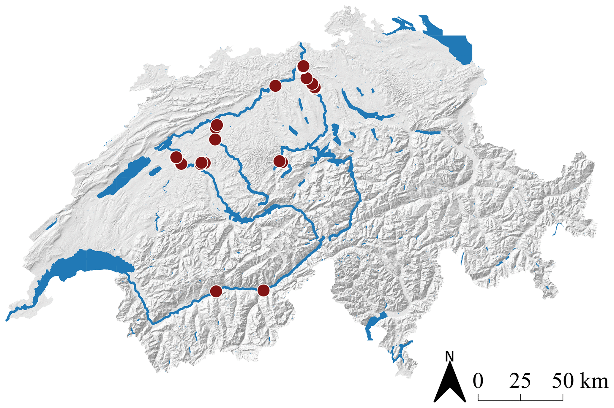
Figure 2Overview map with the 25 ground truth locations of the investigated gravel bars in Switzerland.
One example image tile from each of the 25 sites is shown in Fig. 3. This collection qualitatively highlights the great variety of grain sizes, distributions, and lighting conditions (e.g., shadows, hard and soft light due to different weather conditions). The total number of digital line samples collected per site varies between 4 (Reuss km 021.4) and 212 (Kl. Emme km 030.3), depending on the spatial extent and the variability of grain sizes within the gravel bar.
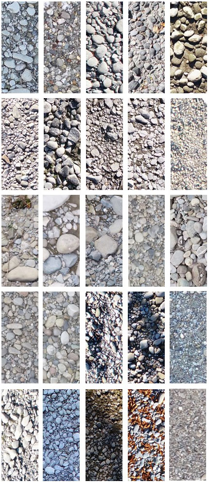
Figure 3Example image tiles (1.25 m×0.5 m) with 0.25 cm ground sampling distance. Each of the 25 example tiles is taken from a different gravel bar.
3.1 UAV imagery
We acquired images with an off-the-shelf consumer UAV, namely, the DJI Phantom 4 Pro. Its camera has a 20 megapixel CMOS sensor (5472×3648 pixels) and a nominal focal length of 24 mm (35 mm format equivalent).5 Flight missions were planned using the flight planner Pix4D capture.6 Images were taken on a single grid, where adjacent images have an overlap of 80 %. To achieve a ground sampling distance of ≈0.25 cm, the flying height was set to 10 m above the gravel bar. This pixel resolution allows the human annotator to identify individual grains as small as 1 cm. Furthermore, to avoid motion blur in the images, the drone was flown at low speed. We generated georeferenced orthophotos with AgiSoft PhotoScan Professional.7
The accuracy of the image scale has a direct effect on the grain size measurement from georeferenced images (Carbonneau et al., 2018). To assure that our digital line samples are not affected by image scale errors, we compare them with corresponding line samples in the field and observe good agreement. Note that absolute georeferencing is not crucial for this study. Because ground truth is directly derived from the orthorectified images, potential absolute georeferencing errors do not affect the processing.
3.2 Annotation strategy
We introduce a new annotation strategy (Fig. 4), called digital line sampling, to label grain sizes in orthorectified images. To allow for a quick adoption of our proposed approach, we closely follow the popular line sampling field method introduced originally by Fehr (1987). Instead of measuring grains in the field, we carry out measurements in images. First, orthorectified images are tiled into rectangular image patches with a fixed size of 1.25 m×0.5 m. We align the major axis with the major river flow, either north–south or east–west. A human annotator manually draws polygons of 100–150 grains along the center line of a tile (Fig. 4a) which takes 10–15 min per sample on average. We asked annotators to imagine the outline of partially occluded grains if justifiable. Afterwards, the minor axis of all annotated grains is measured by automatically fitting a minimum bounding rectangle around the polygons (Fig. 4b). Grain sizes are quantized into 21 bins as shown in Fig. 5, which leads to a relative frequency distribution of grain sizes (Fig. 4c). Line samples are first converted to a quasi-sieve throughput (Fig. 4d) by weighting each bin with the weight (Fehr, 1987), where dmb is the mean diameter per bin and α is set to 2 (assuming no surface armoring). Usually undersampled finer fractions are predicted by a Fuller distribution, which results in the final grading curve (Fig. 4e). This grading curve can either be directly used for fractional bed-load simulations or be used to derive characteristic grain sizes corresponding to the percentiles of the grading curve (Fig. 4f). These are needed, for instance, to calculate the single-grain bed-load transport capacity (d50, d65, dm), to determine the flow resistance (dm, d90), and to describe the degree of surface armoring (d30, d90; Habersack et al., 2011).
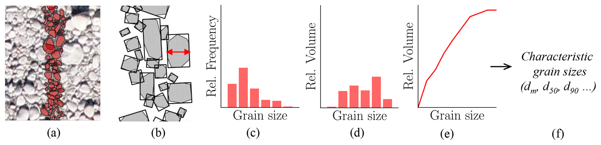
Figure 4Overview of the line sampling procedure. (a) Digital line sample with 100–150 grains, (b) automatic extraction of the b axis, (c) relative frequency distribution of grain sizes, (d) relative volume distribution, (e) grading curve, and (f) characteristic grain sizes (e.g., dm).
Our annotation strategy has several advantages. First, digital line sampling is the one-to-one counterpart of the current state-of-the-art field method in the digital domain. Second, the labeling process is more convenient, as it can be carried out remotely and with arbitrary breaks. Third, image-based line sampling is repeatable and reproducible. Multiple experts can label the exact same location, which makes it possible to compute standard deviations and quantify the uncertainty of the ground truth. Finally, digital line sampling allows one to collect vast amount of training data, which is crucial for the performance of CNNs. For modern machine learning techniques, data quantity is often more important than quality, as shown for example in Van Horn et al. (2015). As it is common machine learning terminology, we use the term ground truth to refer to the manually annotated digital line samples that are used to train and evaluate our model.
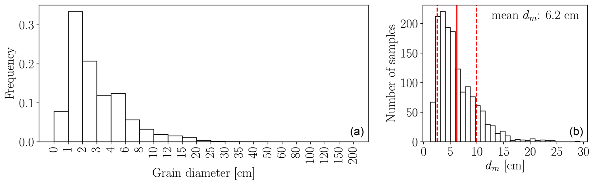
Figure 5Overview of the ground truth data. (a) Average of the 1491 relative frequency distributions; (b) histogram of the respective characteristic mean diameter dm. The solid red line corresponds to the mean dm, and the dashed red lines correspond to mean±SD.
3.3 Ground truth
In total, >180 000 grains over a wide range of sizes have been labeled manually (Fig. 5). Individual grain sizes range from 0.5 to approx. 40 cm. The major mode of individual grain sizes is between 1 and 2 cm, and the minor mode is between 4 and 6 cm. Mean diameters dm per site vary between 1.3 (Aare km 178.0) and 29.3 cm (Grosse Entle km 002.0) with a global mean of all 1491 annotated line samples at 6.2 cm and a global median at 5.3 cm. The distribution of the mean diameters dm (Fig. 5b) follows a bimodal distribution as well. The major mode is around 4 cm and the minor mode around 8 cm. We treat all samples the same and do not further distinguish between shapes when training our CNN model for estimating the size distribution, such that the learned model is universal and applicable to all types of gravel bars. Furthermore, to train a robust CNN, we not only collect easy (clean) samples but also challenging cases with natural disturbances such as grass, leaves, moss, mud, water, and ice.
Many hydrological parameters are continuous by nature and can be estimated via regression. Neural networks are generic machine learning algorithms that can perform both classification and regression. In the following, we discuss details of our methodology for regressing grain size distributions of entire gravel bars from UAV images.
4.1 Image preprocessing
Before feeding image tiles to the CNN, we apply a few standard preprocessing steps. To simplify the implicit encoding of the metric scale into the CNN output, the ground sampling distance (GSD) of the image tiles is unified to 0.25 cm. The expected resolution of a 1.25 m×0.5 m tile after the resampling is 500×200 pixels. Inaccuracies may arise due to rounding effects from the prior cropping. For simplicity, the tile size is cropped to 500×200 pixels. Additionally, horizontal tiles are flipped to be vertical.
Finally, following best practice for neural networks, we normalize the intensities of the RGB channels to be standard normal distributed with mean of 0 and standard deviation of 1, which leads to faster convergence of gradient-based optimization (LeCun et al., 2012). It is important to note that any statistics used for preprocessing must be computed solely from the training data and then applied unaltered to the training, validation, and test sets.
4.2 Regression of grain size distributions with GRAINet
Our CNN architecture, which we call GRAINet, regresses grain size distributions and their characteristic grain sizes directly from UAV imagery. CNNs are generic machine learning algorithms that learn to extract texture and spectral features from raw images to solve a specific image interpretation task. A CNN consists of several convolutional (CONV) layers that apply a set of linear image filter kernels to their input. Each filter transforms the input into a feature map by discrete convolution; i.e., the output is the dot product (scalar product) between the filter values and a sliding window of the inputs. After this linear operation, nonlinear activation functions are applied element-wise to yield powerful nonlinear models. The resulting activation maps are forwarded as input to the next layer. In contrast to traditional image processing, the parameters of filter kernels (weights) are learned from training data. Each filter kernel ranges over all input channels fin and has a size of , where w defines the kernel width. While a kernel width of 3 is the minimum width required to learn textural features, 1×1 filters are also useful to learn the linear combination of activations from the preceding layer.
A popular technique to improve convergence is batch normalization (Ioffe and Szegedy, 2015), i.e., renormalizing the responses within a batch after every layer. Besides better gradient propagation, this also amplifies the nonlinearity (e.g., in combination with the standard rectified linear unit (ReLU) activation function).
Our proposed GRAINet is based on state-of-the-art residual blocks introduced by He et al. (2016). An illustration of our GRAINet architecture is presented in Appendix A in Fig. A1. Every residual block transforms its input using three convolutional layers, each including a batch normalization and a ReLU activation. The first and last convolutional layers consist of filters (CONV 1×1), while the second layer has filters (CONV 3×3). Besides this series of transformations, the input signal is also forwarded through a shortcut, a so-called residual connection, and added to the output of the residual block. This shortcut allows the training signal to propagate better through the network. Every second block has a step size (stride) of 2 so as to gradually reduce the spatial resolution of the input image and thereby increase the receptive field of the network.
We tested different network depths (i.e., number of blocks/layers) and found the following architecture to work best: GRAINet consists of a single 3×3 “entry” CONV layer followed by six residual blocks and a 1×1 CONV layer that generates B final activation maps. These activation maps are reduced to a one-dimensional vector of length B using global average pooling, which computes the average value per activation map. If the final target output is a scalar (i.e., a characteristic grain size like the dm), B is set to 1. To predict a full grain size distribution, B equals the number of bins of the discretized distribution. Finally, the vector is passed through a softmax activation function. The output of that operation can be interpreted as a probability distribution or grain size bins, since the softmax scales the raw network output such that all vector elements lie in the interval [0,1] and sum up to one.8 The total number of parameters of this network architecture is 1.6 million, which is rather lean compared to modern image analysis networks that often have >20 million parameters.
4.2.1 CNN output targets
As CNNs are modular learning machines, the same CNN architecture can be used to predict different outputs. As already described, we can predict either discrete (relative) distributions or scalars such as a characteristic grain size. We thus train GRAINet to directly predict the outputs proposed by Fehr (1987) at intermediate steps (Fig. 4):
- (i)
relative frequency distribution (frequency),
- (ii)
relative volume distribution (volume),
- (iii)
characteristic mean diameter (dm).
4.2.2 Model learning
Depending on the target type (probability distribution or scalar), we choose a suitable loss function (i.e., error metric; Sect. 4.3) that is minimized by iteratively updating the trainable network parameters. We initialize network weights randomly and optimize with standard mini-batch stochastic gradient descent (SGD). During each forward pass the CNN is applied to a batch (subset) of the training samples. Based on these predictions, the difference compared to ground truth is computed with the loss function, which provides the supervision signal. To know in which direction the weights should be updated, the partial derivative of the loss function is computed with respect to every weight in the network. By applying the chain rule for derivatives, this gradient is back-propagated through the network from the prediction to the input (backward pass). The weights are updated with small steps in negative gradient direction. A hyperparameter called the learning rate controls the step size. In the training process, this procedure is repeated iteratively, drawing random batches from the training data. One training epoch is finished once all samples of the training dataset have been fed to the model (at least) once.
We use the ADAM optimizer (Kingma and Ba, 2014) for training, which is a popular adaptive version of standard SGD. ADAM adaptively attenuates high gradients and amplifies low gradients by normalizing the global learning rate with a running average for each trainable parameter. Note that SGD acts as a strong regularizer, as the small batches only roughly approximate the true gradient over the full training dataset. This allows for training neural networks with millions of parameters.
To enhance the diversity of the training data, many techniques for image data augmentation have been proposed, which simulate natural variations of the data. We employ randomly horizontal and vertical flipping of the input images. This makes the model more robust and, in particular, avoids overfitting to certain sun angles with their associated shadow directions.
4.3 Loss functions and error metrics
Various error metrics exist to compare ground truth distributions to predicted distributions. Here, we focus on three popular and intuitive metrics that perform best for our task: the Earth mover's distance (shortened to EMD; also known as the Wasserstein metric), the Kullback–Leibler divergence (KLD), and the Intersection over Union (IoU; also known as the Jaccard index).
The Earth mover's distance (Eq. 1) views two probability density functions (PDFs) p and q as two piles of earth with different shapes and describes the minimum amount of “work” that is required to turn one pile into the other. This work is measured as the amount of moved earth (probability mass) multiplied by its transported distance. In the one-dimensional case, the Earth mover's distance can be implemented as the integral of absolute error between the two respective cumulative density functions (CDFs) P and Q of the distributions (Ramdas et al., 2017). Furthermore, for discrete distributions, the integral simplifies to a sum over B bins.
Alternatively, the Kullback–Leibler divergence (Eq. 2) is widely used in machine learning, because minimizing the forward KLD is equivalent to minimizing the negative likelihood or the cross-entropy (up to a constant). It should be noted though that Kullback–Leibler divergence is not symmetric. For a supervised approach, the forward KLD is used, where p denotes the true distribution and q the predicted distribution. This error metric only accounts for errors in the bins that actually contain a ground truth probability mass, i.e., when p(b)>0. Errors in empty ground truth bins do not contribute to the forward KLD. Therefore, optimizing the forward KLD has a mean-preserving behavior. In contrast, the reverse KLD has a mode-preserving behavior. Note that KLD only accounts for errors in bins containing ground truth probability mass. Thus, the overestimation of empty bins does not directly contribute to the error metric, but as we treat the grain size distribution as a probability distribution, this displaced probability mass is missing in the bins that are taken into account.9
In contrast to the EMD and KLD, the Intersection over Union (Eq. 3) is an intuitive error metric that is maximized and ranges between 0 and 1. While it is often used in object detection or semantic segmentation tasks, it allows one to compare two 1D probability distributions as follows:
During the training process the loss function (Eq. 4) simply averages the respective error metric over all samples within a training batch. To evaluate performance, we average the error over the unseen test dataset:
where D corresponds to the error metric, f denotes the CNN model, N the number of samples, xi the input image tile, yi the ground truth PDF or CDF, and f(xi) the predicted distribution.
To optimize and evaluate CNN variants that directly predict scalar values (like, for example, GRAINet, which directly predicts the mean diameter dm), we investigate two loss functions: the mean absolute error (MAE, also known as L1 loss, Eq. 5) and the mean squared error (MSE, also known as L2 loss, Eq. 6).
Furthermore, we evaluate the model bias with the mean error (ME):
where a positive mean error indicates that the prediction is greater than the ground truth.
4.4 Evaluation strategy
The trained GRAINet is quantitatively and qualitatively evaluated on a holdout test set, i.e., a portion of the dataset that was not seen during training. We analyze error cases and identify limitations of the proposed approach. Finally, with our image-based annotation strategy, multiple experts can label the same sample, which we exploit to relate the model performance to the variation between human expert annotations.
4.4.1 Tenfold cross-validation
To avoid any train–test split bias, we randomly shuffle the full dataset and create 10 disjoint subsets, such that each sample is contained only in a single subset. Each of these subsets is used once as the hold-out test set, while the remaining nine subsets are used for training GRAINet. The validation set is created by randomly holding out 10 % of the training data and used to monitor model performance during training and to tune hyperparameters. Results on all 10 folds are combined to report overall model performance.
4.4.2 Geographical cross-validation
Whether or not a model is useful in practice strongly depends on its capability to generalize across a wide range of scenes unseen during training. Modern CNNs have millions of parameters, and in combination with their nonlinear properties, these models have high capacity. Thus, if not properly regularized or if trained on a too small dataset, CNNs can potentially memorize spurious correlations specific to the training locations which would result in poor generalization to unseen data. We are particularly interested to know if the proposed approach can be applied to a new (unseen) gravel bar. In order to validate whether GRAINet can generalize to unseen river beds, we perform geographical cross-validation. All images of a specific gravel bar are held out in turn and used to test the model trained on the remaining sites.
4.4.3 Comparison to human performance
The predictive accuracy of machine learning models depend on the quality of the labels used for training. In fact, label noise that would lead to inferior performance of the model is introduced partially by the labeling method itself. Grain annotation in images is somewhat subjective and thus differs across different annotators. The advantage of our digital line sampling approach is that multiple experts can perform the labeling at the exact same location, which is infeasible if done in situ, because line sampling is disruptive and cannot be repeated. We perform experiments to answer two questions. First, what is the variation of multiple human annotations? Second, can the CNN learn a proper model, despite the inevitable presence of some label noise? We randomly selected 17 image tiles that are labeled by five skilled operators, who are familiar with traditional line sampling in the field.
4.5 Final products
On the one hand, by combining the output of GRAINet trained to either predict the frequency or the volume distribution with the approach proposed by Fehr (1987), we can obtain the grading curve (cumulative volume distribution) as well as the characteristic grain sizes (e.g., dm). On the other hand, GRAINet can also be trained to directly predict characteristic grain sizes. The characteristic grain size dm is only one example of how the proposed CNN architecture can be adapted to predict specific aggregate parameters. Ultimately, the GRAINet architecture allows one to predict grain size distributions or characteristic grain sizes densely for entire gravel bars, with high spatial resolution and at large scale, which makes the (subjective) choice of sampling locations redundant. These predictions can be further used to create two kinds of products, illustrated in Fig. 1:
-
dense high-resolution maps of the spatial distribution of characteristic grain sizes,
-
grading curves for entire gravel bars, by averaging the grading curves at individual line samples.
4.6 Experimental setup
For all experiments, the data are separated into three disjoint sets: a training set to learn the model parameters, a validation set to tune hyperparameters and to determine when to stop training to avoid overfitting, and a test set used only to assess the performance of the final model.
The initial learning rate is empirically set to 0.0003, and each batch contains eight image tiles, which is the maximum possible within the 8 GB memory limit of our GPU (Nvidia GTX 1080). While we run all experiments for 150 epochs for convenience, the final model weights are not defined by the last epoch but taken from the epoch with the lowest validation loss. An individual experiment takes less than 4 h to train. Due to the extensive cross-validation, we parallelize across multiple GPUs to run the experiments in reasonable time.
Our proposed GRAINet approach is quantitatively evaluated with 1491 digital line samples collected on orthorectified images from 25 gravel bars located along six rivers in Switzerland (Sect. 3). We first analyze the quality of the collected ground truth data by comparing our digital line samples with field measurements. We then evaluate the performance of GRAINet for estimating the three different outputs:
- i.
relative frequency distribution (frequency),
- ii.
relative volume distribution (volume),
- iii.
characteristic mean diameter (dm).
In order to get an empirical upper bound for the achievable accuracy, we compare the performance of GRAINet with the variation of repeated manual annotations. All reported results correspond to random 10-fold cross-validation, unless specified otherwise. In addition, we analyze the generalization capability of all three GRAINet models with the described geographical cross-validation procedure and investigate the error cases to understand the limitations of the proposed data-driven approach. Finally, as our CNN does not explicitly detect individual grains, we investigate the possibility to estimate grain sizes from lower image resolutions.
5.1 Quality of ground truth data
We evaluate the quality of the ground truth data in two ways. First, the digital line samples are compared with state-of-the-art in situ line samples from field measurements. Second, the label uncertainty is studied by comparing repeated annotations by multiple skilled operators.

Figure 6Comparison of digital line samples with 22 in situ line samples collected in the field.
5.1.1 Comparison to field measurements
From 22 out of the 25 gravel bars, two to three field measurements from experienced experts were available (see Fig. 6). These field samples were measured according to the line sampling proposed by Fehr (1987). To compare the digital and in situ line samples, we derive the dm values and compare them at the gravel bar level, because the field measurements are only geolocalized to that level. Some field measurements were accomplished a few days apart from the UAV surveys. We expect grain size distributions to remain unchanged, as no significant flood event occurred during that time. Figure 6 indicates that the field-measured dm is always within the range of the values derived from the digital line samples. Furthermore, the mean of the field samples agrees well with the mean of the digital samples. Comparing the mean dm derived from field and digital line samples across the 22 bars results in a mean absolute error of 0.9 cm and in a mean error (bias) of −0.3 cm, which means that the digital dm is on average slightly lower than the dm values derived from field samples. The wide range of the digital line samples emphasizes that the choice of a single line sample in the field is very crucial and that it requires a lot of expertise to chose a few locations that yield a meaningful sample of the entire gravel bar population. Considering that the field samples are unavoidably affected by the selected location and also by operator bias (Wohl et al., 1996), we conclude that within reasonable expectations the digital line samples are in good agreement with field samples and constitute representative ground truth data. Nevertheless, to better understand the difference between digital line sampling and field sampling, a new dataset should be created in the future, where field samples are precisely geolocated to allow for a direct comparison at the tile level.
5.1.2 Label uncertainty from repeated annotations
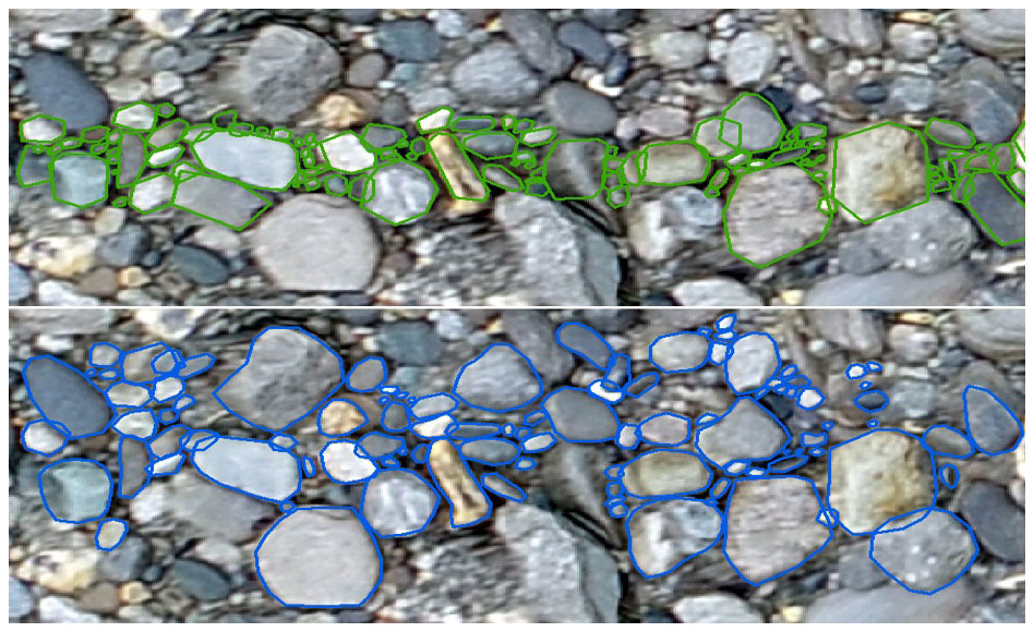
We compute statistics of three to five repeated annotations of 17 randomly selected image tiles (see Table C1 in the Appendix) to analyze the (dis)agreement between human annotators. The standard deviation of dm across different annotators varies between 0.1 (Aare km 172.2) and 2.0 cm (Rhone km 083.3); the average standard deviation is 0.5 cm. Although these 17 samples are too few to compute reliable statistics, we get an intuition for the uncertainty of the digital line samples. Figure 7 shows two different annotations for the same image tile, to demonstrate the variation introduced by the subjective selection of valid grains. While the distribution in the upper annotation (in green) contains a larger fraction of smaller grains following closely the center line, the lower annotation (in blue) contains a larger fraction of larger grains, including some further away from the center line.
Recall that this comparison of multiple annotators is only possible because digital line sampling is nondestructive. In contrast, even though variations of similar magnitude are expected in the field, a quantitative analysis is not easily possible. Nevertheless, Wohl et al. (1996) found that sediment samples are biased by the operator. Although CNNs are known to be able to handle a significant amount of label noise if trained on large datasets (Van Horn et al., 2015), the uncertainty of the manual ground truth annotations is also present in the test data and therefore represents a lower bound for the performance of the automated method. Therefore, while we do not expect the label noise to degrade the CNN training process, we do not expect root-mean-square errors below 0.5 cm due to the apparent label noise in the test data.
5.2 Estimation of grain size distributions
As explained in Sect. 3.2, the process of obtaining a grading curve according to Fehr (1987) involves several empirical steps (Fig. 4). In this processing pipeline, the relative frequency distribution can be regarded as the initial measurement. However, as the choice of the proper CNN target is a priori not clear, we investigate the two options to estimate (i) the relative frequency distribution and (ii) the relative volume distribution. In the latter version, the CNN implicitly learns the conversion from frequency to fraction-weighted quasi-sieve throughput, making that processing step obsolete. We experiment with three loss functions to train GRAINet for the estimation of discrete target distributions: the Earth mover's distance (EMD), the Kullback–Leibler divergence (KLD), and the Intersection over Union (IoU). For each trained model, all three metrics are reported in Table 1. The standard deviation quantifies the performance variations across the 10 random data splits. Theoretically, one would expect the best performance under a given error metric D from the model trained to optimize that same metric; i.e., the best performance per column should be observed on the diagonals in the two tables. Note that each error measure lives in its own space; numbers are not comparable across columns.
Table 1Results for GRAINet regressing (a) the relative frequency distribution and (b) the relative volume distribution. Mean and standard deviation (in parenthesis) for the random 10-fold cross-validation. The rows correspond to the CNN models trained with the respective loss function. Arrows indicate if the error metric is minimized (↓, lower is better) or maximized (↑, higher is better).

5.2.1 Regressing the relative frequency distribution
When estimating the relative frequency distribution, all three loss functions yield rather similar mean performance, in all three error metrics (Table 1a). The lowest KLD (mean of 0.13) and the highest IoU (mean of 0.73) are achieved by optimizing the respective loss function, whereas the lowest EMD is also achieved by optimizing the IoU. However, all variations are within 1 standard deviation. The KLD is slightly more sensitive than the other loss functions, with the largest relative difference (0.13 vs. 0.16) corresponding to a 23 % increase. All standard deviations are 1 order of magnitude smaller than the mean, meaning that the reported performance is not significantly affected by the specific splits into training and test sets.
5.2.2 Regressing the relative volume distribution
The regression performance for the relative volume distribution is presented in Table 1b. Here, the best mean performance is indeed always achieved by optimizing the respective loss function. The relative performance gap under the KLD error metric increases to 250 %, with 0.32 when trained with the KLD loss vs. 0.80 with the IoU loss. Also the standard deviation of the KLD between cross-validation folds exhibits a marked increase.
5.2.3 Performance depending on the GRAINet regression target
In comparison to the values reported in Table 1a, the KLD on the volume seems to be even more sensitive regarding the choice of the optimized loss function. Furthermore, all error metrics are worse when estimating the volume instead of the frequency distribution: the best EMD increases from 0.42 to 0.65, the KLD increases from 0.13 to 0.32, and the best IoU decreases from 0.73 to 0.61.
Looking at the difference between the frequency and the volume distribution, we see a general shift of the probability mass to the right-hand side of the distributions, which is clearly visible in Fig. 8c and f. While the frequency is generally smoothly decreasing to zero probability mass towards the larger grain size fractions of the distribution, the volume has a very sharp jump at the last bin (Fig. 8c and f), where the largest grain – often only a single one (Fig. 9b and f) – has been measured.
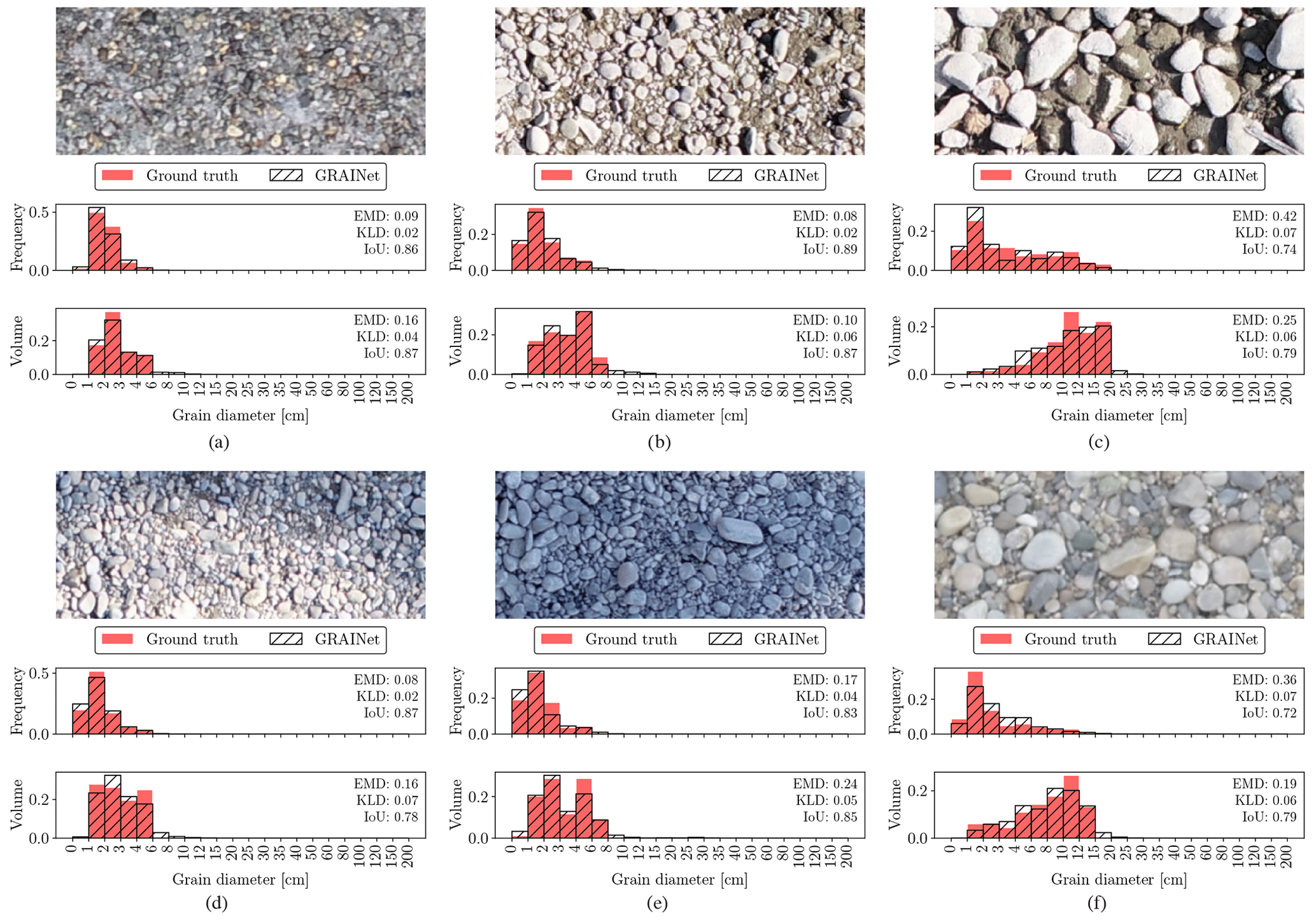
Figure 8Example image tiles where the GRAINet regression of the relative frequency and volume distributions yields good performance.
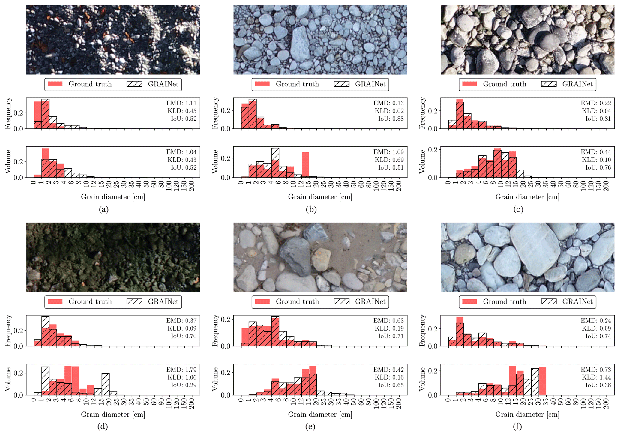
Figure 9Error cases where the GRAINet regression of the relative frequency and volume distributions fails.
Figure 8 displays examples of various lighting conditions and grain size distributions, where GRAINet yields a good performance for both targets. On the other hand, the error cases in Fig. 9 represent the limitations of the model. While, for example, extreme lighting conditions deteriorate the performance on both targets similarly (Fig. 9a), the rare radiometry caused by moss (Fig. 9d) has a stronger effect on the volume prediction.
Comparing the predictions with the ground truth distributions in Fig. 9, the GRAINet predictions seem to be generally smoother for both frequency and volume. More specifically, the predicted distributions have longer tails (Fig. 9a, c, and e) and closed gaps of empty bins (Fig. 9f).
In combination with the smoother output of the CNN, the sharp jump in the volume distribution could be an explanation for the generally worse approximation of the volume compared to the frequency.
5.2.4 Learned global texture features
To investigate to what degree the texture features learned by the CNN are interpretable with respect to grain sizes, we visualize the activation maps of the last convolution layer, before the global average pooling, in Fig. 10. In that layer of the CNN there is one activation map per grain size bin, and those maps serve as a basis for regressing the relative frequencies. Therefore, each of these 21 activation maps corresponds to a specific bin of grain sizes, with bin 0 for the smallest grains and bin 20 for the largest ones. Light colors denote low activation, and darker red denotes higher activation. To harmonize the activations to a common scale, [0,1], for visualization, we pass the maps through a softmax over bins. This can be interpreted as a probability distribution over grain size bins at each pixel of the downsampled patch. The resulting activation maps in Fig. 10 exhibit plausible patterns, with smaller grains activating the corresponding lower bin numbers.
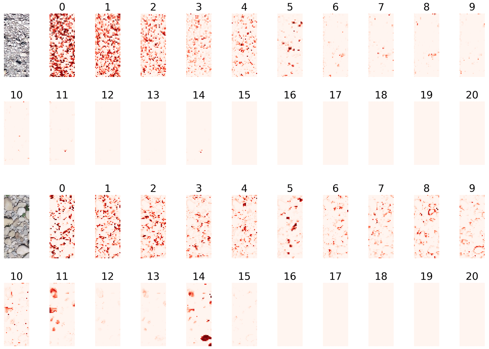
Figure 10Activation maps after the last convolutional layer for two examples. Each of the 21 maps corresponds to a specific histogram bin of the grain size distribution, where bin 0 corresponds to the smallest and bin 20 to the largest grains. Light colors are low activation, and darker red denotes higher activation.
5.2.5 Grading curves for entire gravel bars
We compute grading curves from the predicted relative frequency and volume distributions as described in Sect. 3.2. Furthermore, we average the individual curves to obtain a single grading curve per gravel bar. We show example grading curves obtained with the three different loss functions in Fig. 11. The top row shows a distribution of rather fine grains, while the bottom row represents a gravel bar of coarse grains. Regarding the fine gravel bar (Fig. 11a–c), the difference between the three loss functions is hard to observe. Yet, there is a tendency of overestimating the coarse fraction if optimizing for KLD. However, only KLD can reproduce the grading curve of the coarse gravel bar reasonably well (Fig. 11d–f). Overall, the experiments indicate that the KLD loss yields best performance for all three error metrics. Thus, to assess the effect of the target choice (frequency vs. volume) on the final grading curves of all 25 gravel bars, we use the GRAINet trained with the KLD loss (Fig. 12). Both models approximate the ground truth curves well and are able to reproduce various shapes (e.g., Aare km 171.2 vs. Reuss km 001.3) . However, the grading curves derived from the predicted frequency distribution (dashed curves) tend to overestimate higher percentiles (e.g., Aare km 171.0).
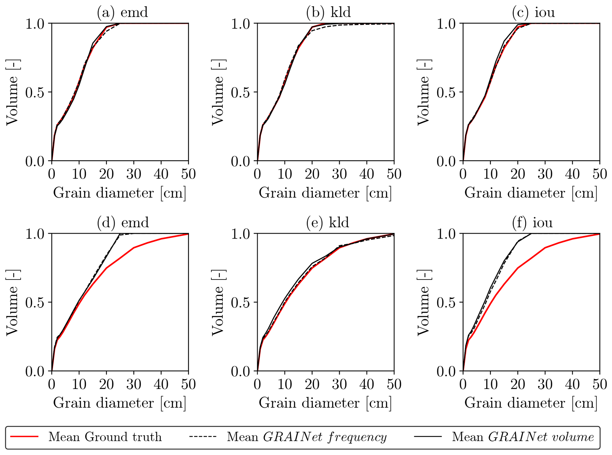
Figure 11Grading curves resulting from optimizing different loss functions (from left to right: EMD, KLD, IoU) for two example gravel bars, namely, Gr. Entle km 002.0 (a–c) and Reuss km 001.6 (d–f).
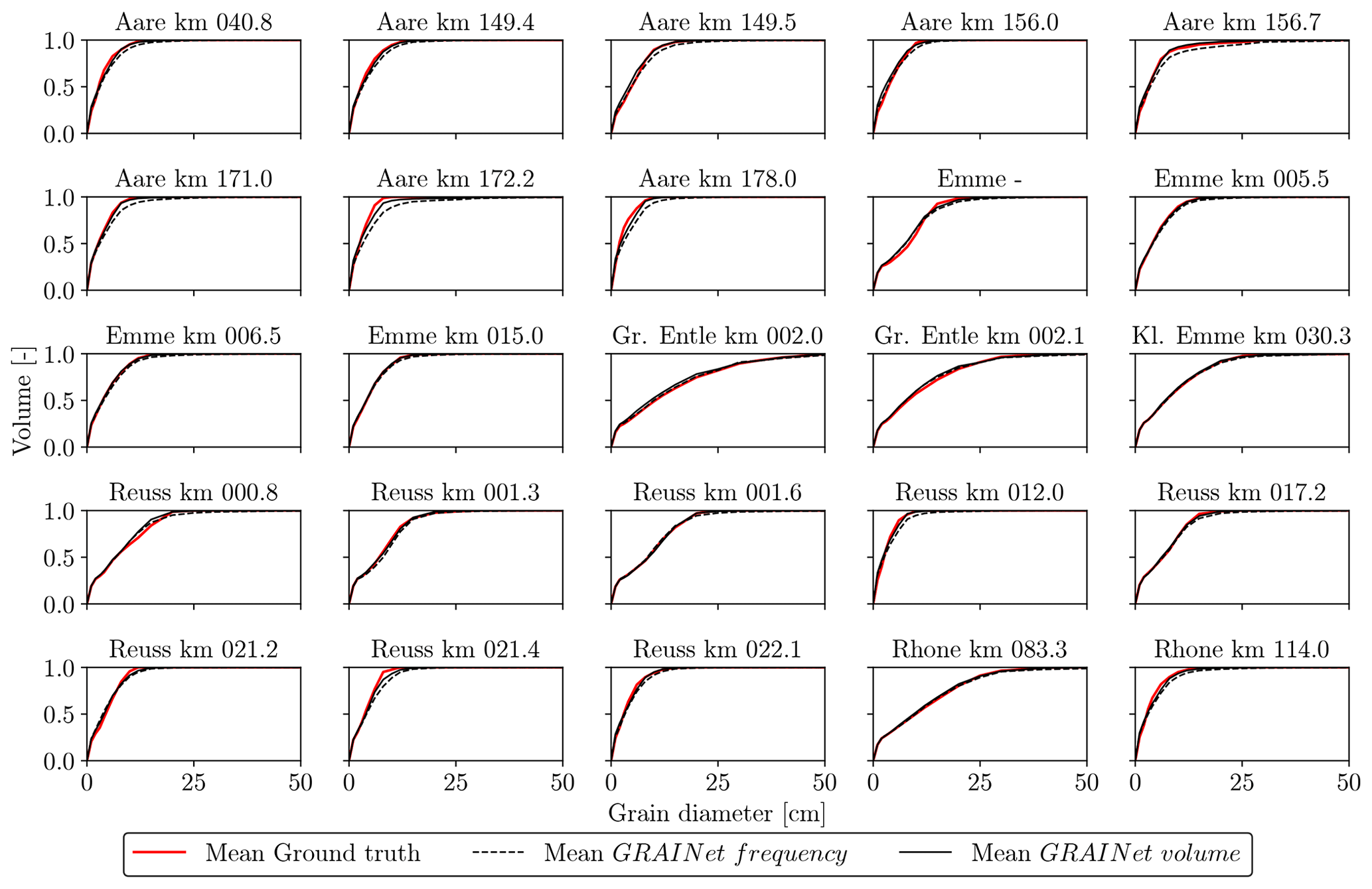
Figure 12Grading curves of the 25 gravel bars, estimated with random 10-fold cross-validation.
This qualitative comparison indicates that regressing the volume distribution with GRAINet yields slightly better grading curves than for the frequency distribution. If computing the grading curve from the predicted frequency distribution, small errors in the bins with larger grains are propagated and amplified in a nonlinear way due to the fraction-weighted transformation described in Sect. 3.2. In contrast, the volume distribution already includes this nonlinear transformation and consequently errors are smaller.
5.3 Estimation of characteristic grain sizes
Characteristic grain sizes can be derived from the predicted distributions, or GRAINet can be trained to directly predict variables like the mean diameter dm as scalar outputs.
5.3.1 Regressing the mean diameter dm
We again analyze the effect of different loss functions, namely, the mean squared error (MSE) and the mean absolute error (MAE) when training GRAINet to estimate dm end-to-end; see Table 2. Note that minimizing MSE is equivalent to minimizing the root-mean-square error (RMSE). Optimizing for MAE achieves slightly lower errors under both metrics (3.04 cm2 and 0.99 cm, respectively). However, optimizing for MAE results in significantly stronger bias, with a ME of −0.11 cm (underestimation) compared to 0.02 cm for the MSE. As for practical applications a low bias is considered more important, we use GRAINet trained with the MSE loss for further comparisons. This yields a MAE of 1.1 cm (18 %) and an RMSE of 1.7 cm (27 %), respectively. Analogous to Buscombe (2013), the corresponding normalized errors in parenthesis are computed by dividing through the overall mean dm of 6.2 cm (Fig. 5).
Table 2Results for GRAINet regressing the mean diameter dm [cm]. Mean and standard deviation (in parenthesis) for the random 10-fold cross-validation. The rows correspond to the CNN models trained with the respective loss function. While both MSE and MAE are minimized (↓), the ME is optimal with zero bias (0).
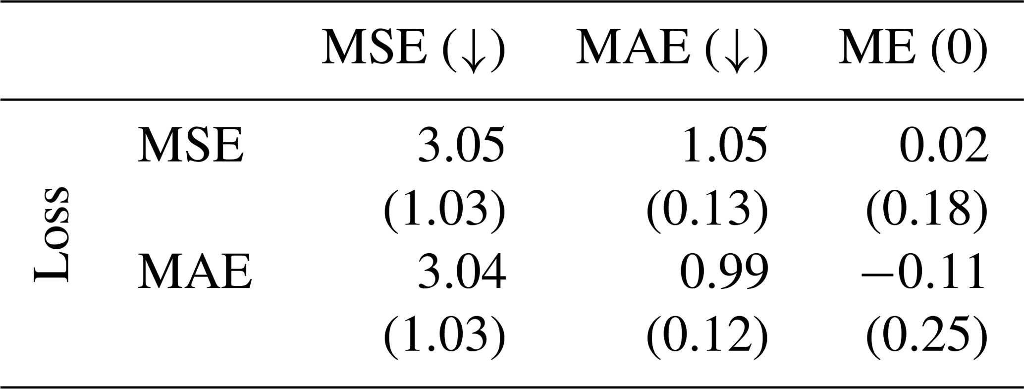

Figure 13Scatter plots of the estimated dm [cm] from the three GRAINet outputs: frequency, volume, and dm (left to right). The ground truth dm is on the horizontal axis, and predicted dm is on the vertical axis.
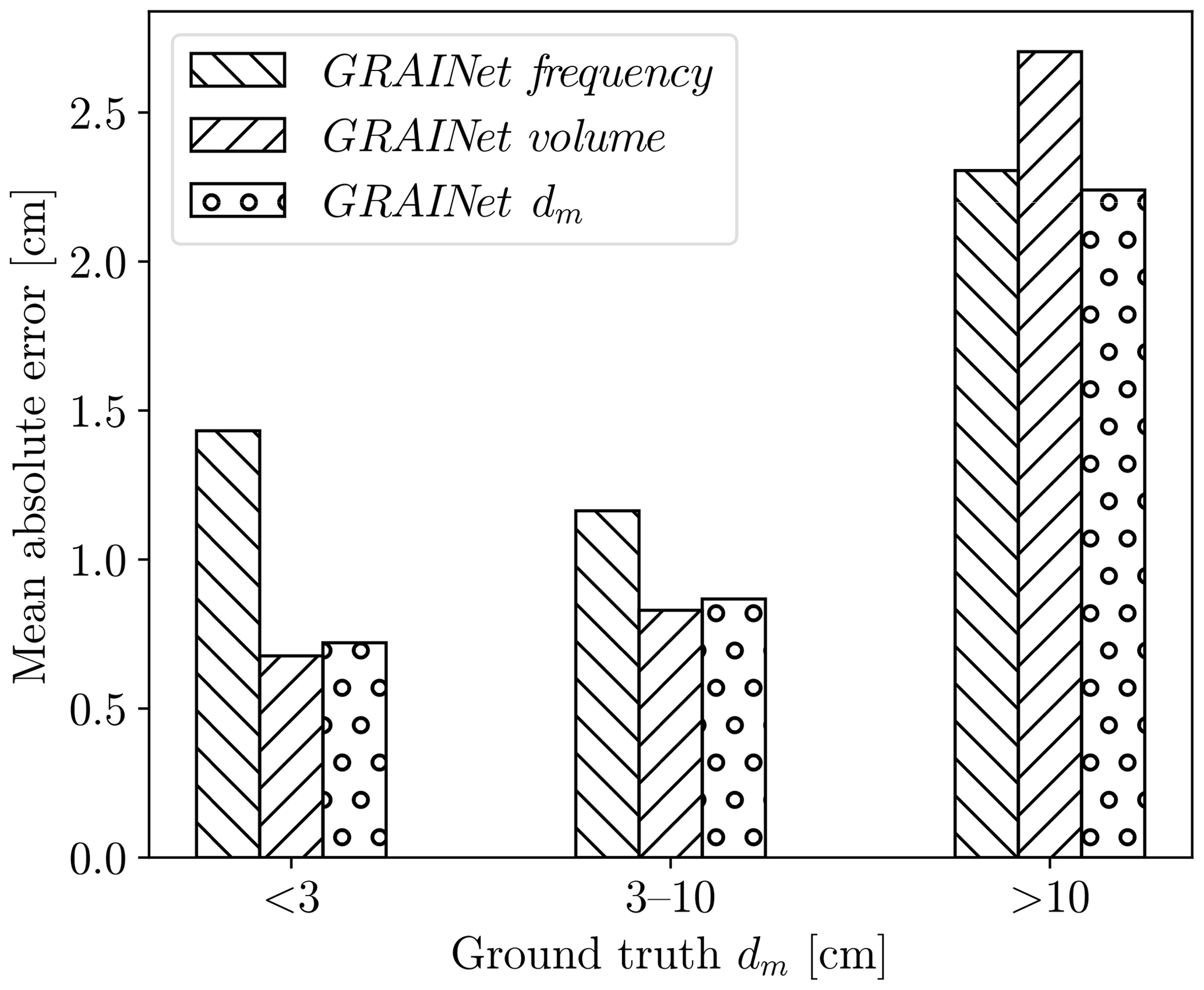
Figure 14Mean absolute error of the predicted dm for three dm-categories: <3 cm, 3–10 cm, and >10 cm
5.3.2 Performance for different regression targets
If our target quantity is the dm, we now have different strategies. The classical multistep approach would be to measure frequencies, convert them to volumes, and derive the dm from those. Instead of estimating the frequency, we could also directly estimate volumes or predict the dm directly from the image data. Which approach works best? Based on the results shown so far (Tables 1 and 2), we compare the dm values derived from frequency and volume distributions (trained with KLD) to the end-to-end prediction of dm (trained with MSE); see Fig. 13. Regardless of the GRAINet target, the ME lies within ±0.7 cm, the MAE is smaller than 1.5 cm, and the absolute dispersion increases with increasing dm. With ground truth dm values ranging from 1.3 to 29.3 cm, only the end-to-end dm prediction covers the full range down to 1.3 and up to 24 cm. In contrast, the smallest dm values derived from the predicted frequency and volume distributions are 2.9 and 2.3 cm, respectively. That is, dm values <3.0 cm tend to be overestimated when derived from intermediate histograms. This is mainly due to unfavorable error propagation, as slight overestimates of the larger fractions are amplified into more serious overestimates of the characteristic mean diameter dm. While the dm derived from the volume prediction yields a comparable MAE of 0.7 cm for ground truth dm<3 cm, only the end-to-end regression is able to predict extreme, small, but apparently rare, values (Fig. 14). The end-to-end dm regression yields a MAE of 0.9 cm for dm values between 3 and 10 cm and 2.2 cm for values >10 cm.
We conclude that end-to-end regression of dm performs best. It achieves the lowest overall MAE (<1.1 cm), and at the same time it is able to correctly recover dm below 3.0 cm.
5.3.3 Mean dm for entire gravel bars
Robust estimates of characteristic grain sizes (e.g., dm, d50) for entire gravel bars or a cross-sections are important to support large-scale analysis of grain size characteristics along gravel-bed rivers (Rice and Church, 1998; Surian, 2002; Carbonneau et al., 2005). To assess the performance of GRAINet for this purpose, the GRAINet end-to-end dm predictions are averaged over each gravel bar and compared with the respective mean dm of the digital line samples (Fig. 15). The performance averaged over all 25 gravel bars results in a MAE of 0.3 cm and a ME of 0.1 cm. The error is <1 cm for all gravel bars, even for the bars at the rivers Gr. Entle and Rhone, which have a mean ground truth dm>10 cm (Table B1). For 13 gravel bars, the error is below ±0.2 cm.
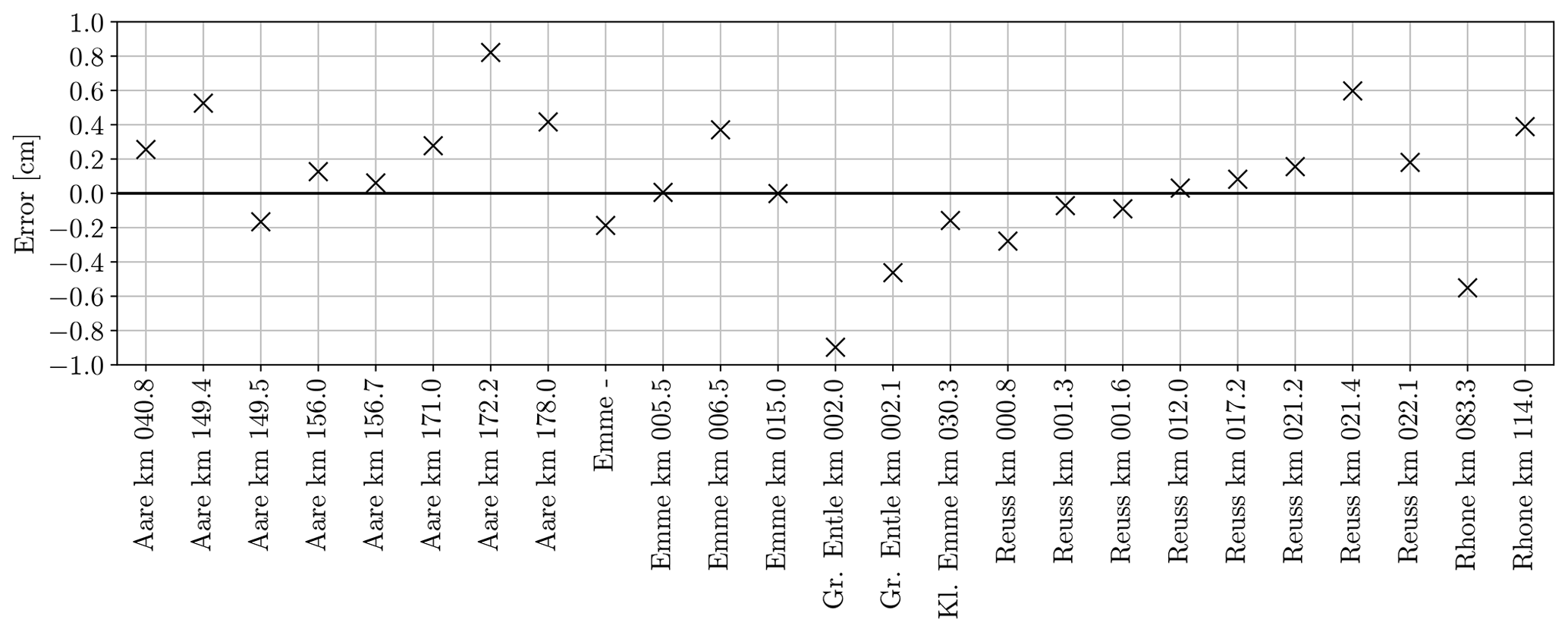
Figure 15Error of the mean dm per gravel bar derived from the GRAINet end-to-end dm predictions.
5.3.4 Comparison to human performance
The average standard deviation σ of dm from repeated digital line samples accounts for 0.5 cm (see Sect. 5.1) for 17 randomly selected tiles. In comparison, regressing dm with GRAINet yields a root-mean-square error (RMSE) of 1.7 cm, of which ≈30 % can be explained by the label noise in the test data. We illustrate the performance of GRAINet versus human performance in Fig. 16. The predicted dm values lie within 1σ for 9 tiles (53 %) and within 2σ for 12 tiles (70 %).
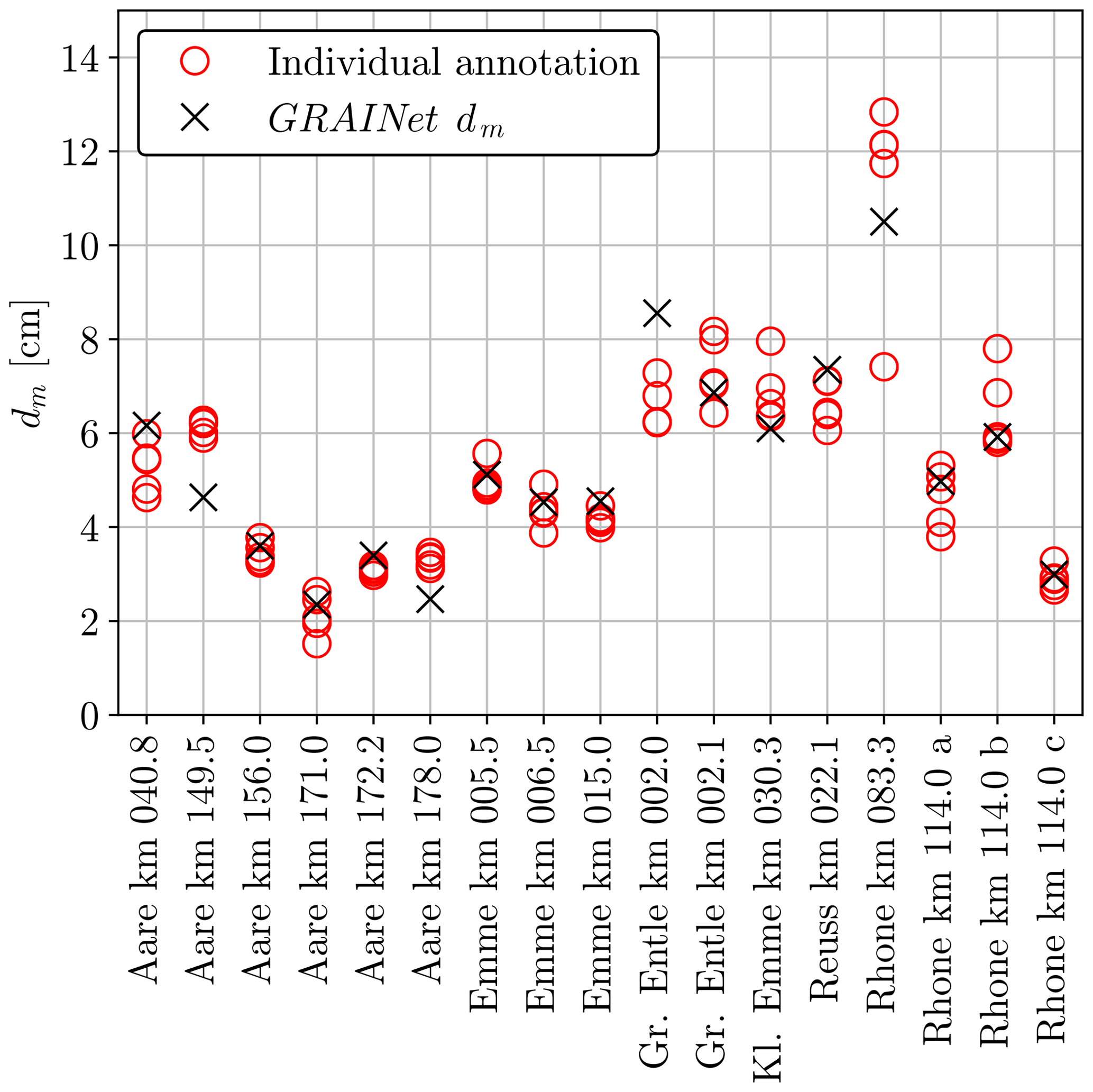
Figure 16Variation of dm annotated by three to five different human experts, compared to end-to-end dm regression of GRAINet.
5.3.5 High-resolution grain size maps
GRAINet offers the possibility to predict and map characteristic grain sizes densely for entire gravel bars with high resolution (1.25 m×0.5 m). Three example maps are presented in Fig. 17. The mean ground truth dm per gravel bar varies between 3.0 cm (Reuss km 012.0, a and b), 3.3 cm (Aare km 171.0, c and d), and >10 cm (Gr. Entle km 002.1, e and f). For all three examples, the river flows northwards.
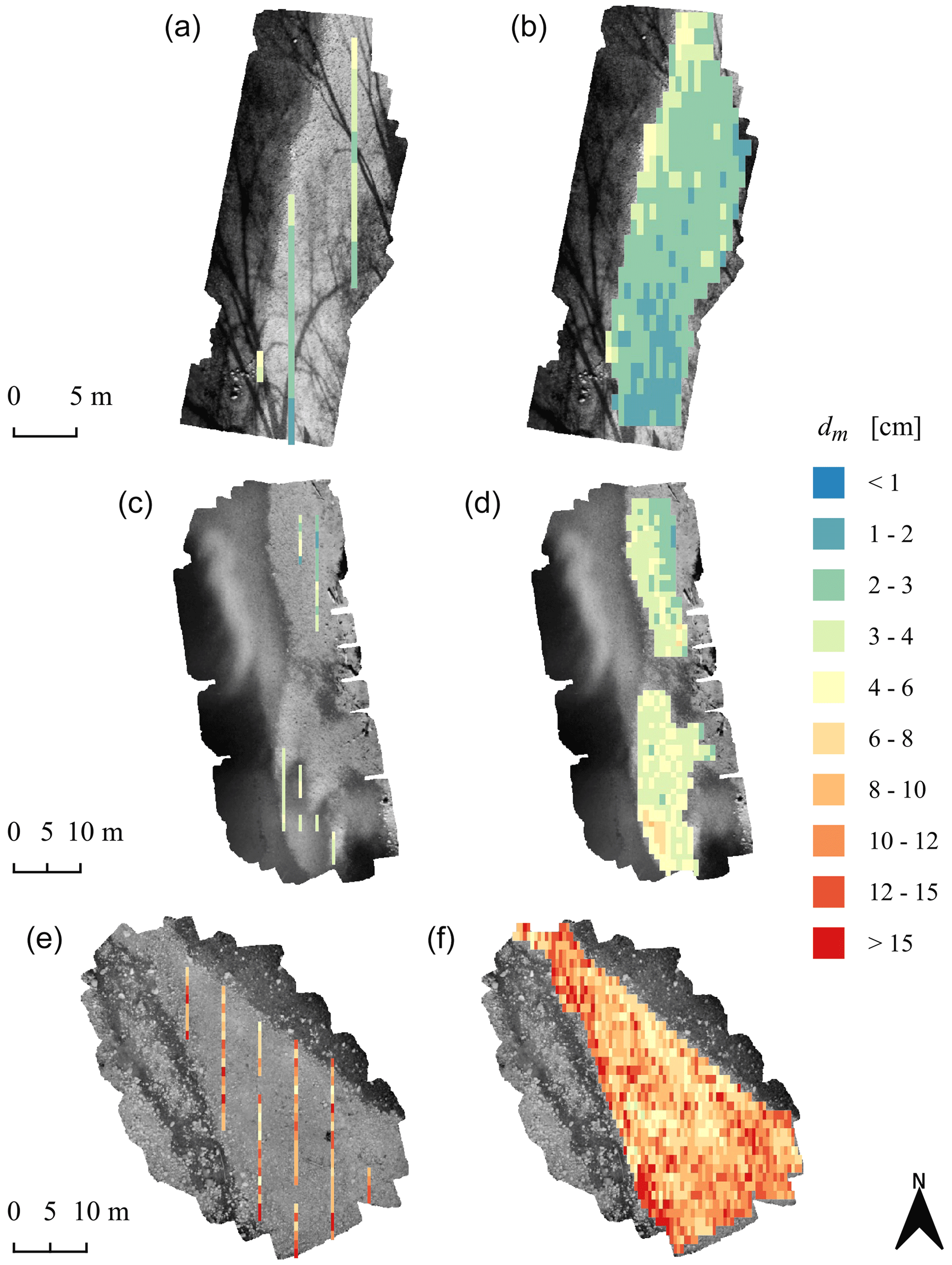
Figure 17Maps of the characteristic mean diameter dm, manually labeled ground truth, i.e., digital line samples (a, c, e) and GRAINet end-to-end dm predictions (b, d, e). Gravel bars (top to bottom): Reuss km 012.0, Aare km 171.0, and Grosse Entle km 002.1. The background is a grayscale version of the input UAV image.
Obviously, the map created with GRAINet offers full coverage of the entire gravel bar, whereas digital line samples deliver only a sparse map. Not only do we see that GRAINet successfully predicts the spatial distribution of the dm in the ground truth but it also reveals spatial patterns at a finer resolution.
Hence, GRAINet enables not only the assessment of difference between gravel bars but also the spatial variability and heterogeneity of dm values within a single gravel bar. Despite a similar mean dm of approximately 3 cm, the spatial layout differs greatly between Reuss (top) and Aare (center), which becomes clear when looking at dense maps of the complete gravel bars. Such sorting effects are not observable in the third example of Gr. Entle.
5.4 Generalization across gravel bars
We study the generalization capability of GRAINet to an unseen gravel bar with geographical cross-validation for regressing the grain size distribution and dm. Note that we cannot completely isolate the effect of unseen grain size distributions from the influence of unseen imaging conditions, as each gravel bar was captured in a separate survey.
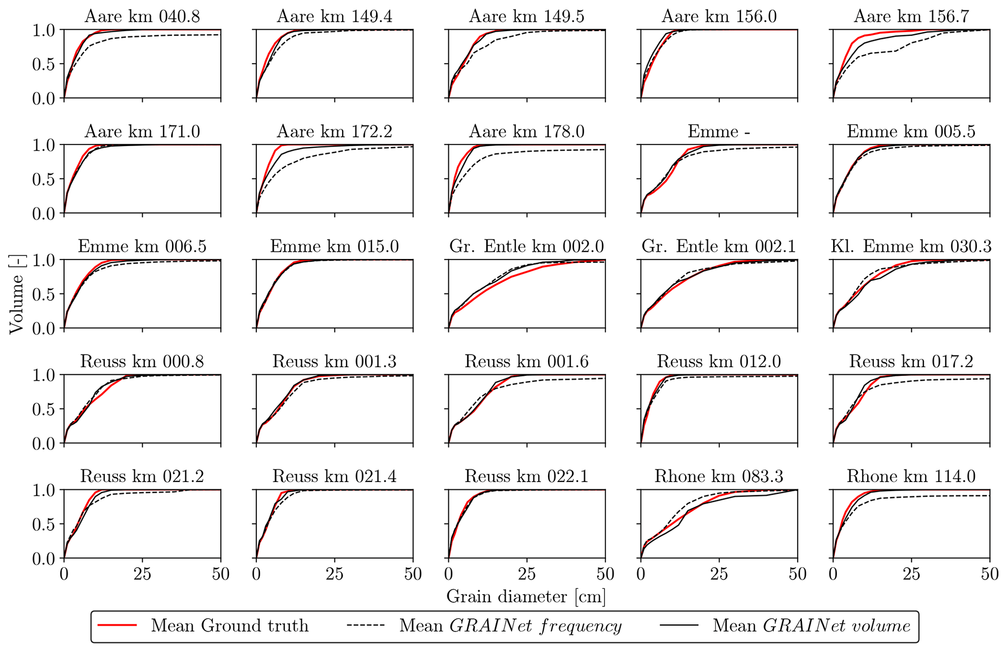
Figure 18Grading curves of the 25 gravel bars, estimated with geographical cross-validation.
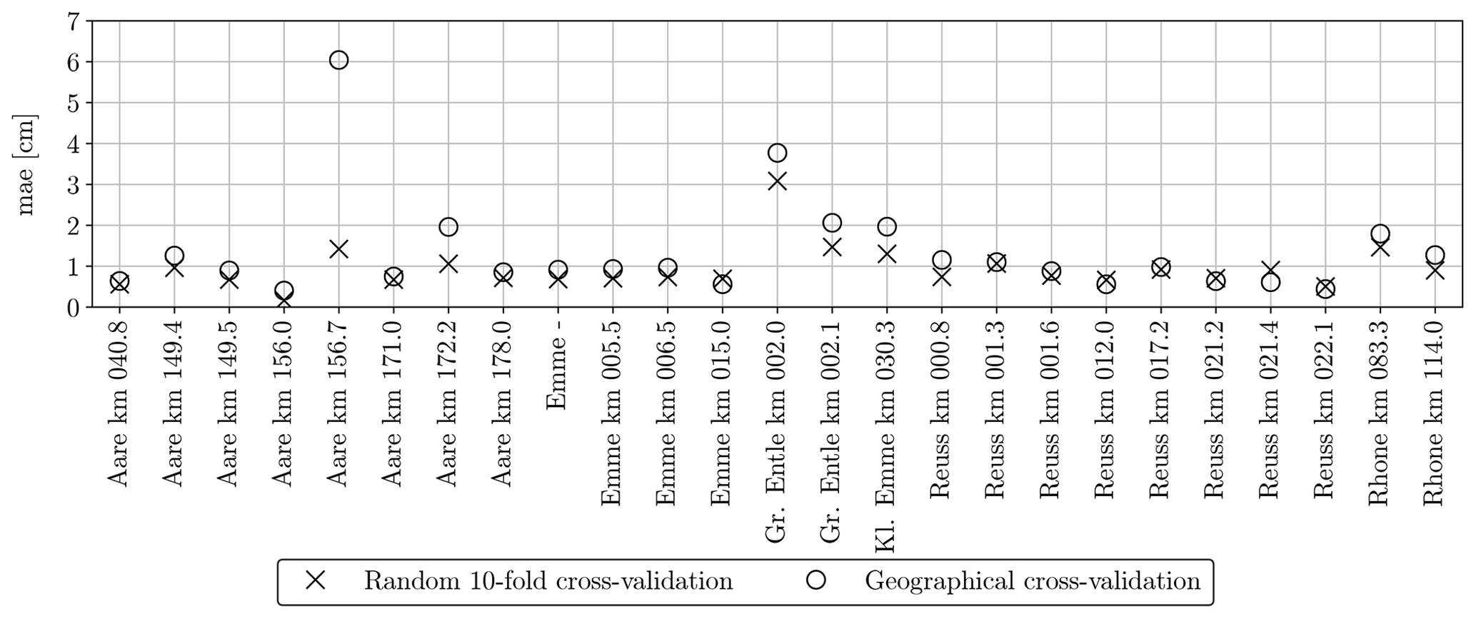
Figure 19Mean absolute error of the GRAINet end-to-end dm regression per gravel bar (random and geographical cross-validation).
5.4.1 Grading curves
Grading curves for all 25 gravel bars are given in Fig. 18. A qualitative comparison to Fig. 12 shows the effect of not seeing a single sample of the respective gravel bar during the training. The grading curves derived from the predicted frequency distribution seem to be less robust, and overestimation of higher percentiles is increased for more than 50 % of all gravel bars. Exceptions are Gr. Entle km 002.0 and Rhone km 083.3, where all percentiles are underestimated. As no striking differences are visible for about 20 gravel bars, we can say that the grading curves derived from the predicted volume distribution generalize (still) well in 80 % of the cases.
5.4.2 Mean diameter dm
We also study the generalization regarding the estimation of the dm (Figs. 19 and D1). The MAE of the random splits is <1 cm for 18 bars and <2 cm for 24 bars. When GRAINet is tested on unseen gravel bars (geographical cross-validation), the MAE does generally increase leading to only 15 bars <1 cm and 19 <2 cm. We observe the largest performance drop for Aare km 156.7, where the MAE increases from 1.4 cm (random 10-fold cross-validation) to 6 cm (geographical cross-validation). On this particular gravel bar, several tiles contain some wet and even flooded grains. Although the refraction of the shallow water could in principle change the apparent grain size, it is most likely not the main reason for the poor generalization. Rather, the model has simply not learned the radiometric characteristics of wet grains, as there are not any among the samples from the other bars used for training.
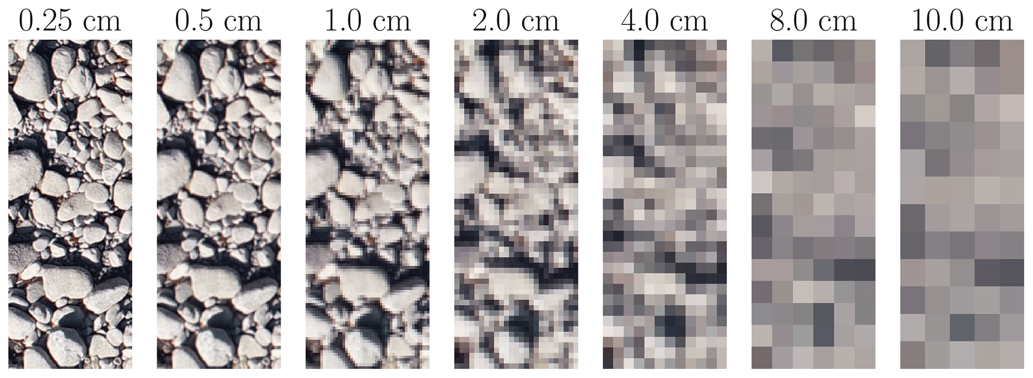
Figure 20Example image tile resampled to lower resolutions. Left to right: full resolution of 0.25 cm and tested downsampling factors: 2, 4, 8, 16, 32, and 40, corresponding to 0.5, 1.0, 2.0, 4.0, 8.0, and 10.0 cm, respectively.
5.5 Effect of the image resolution
GRAINet does not explicitly detect individual grains but learns to identify global texture patterns. It thus seems feasible to apply GRAINet to images of lower resolution, where individual grains would no longer be recognizable by a human annotator (see example in Fig. 20). To simulate that situation, we bilinearly downsampled the original image resolution of 0.25 cm by factors of 2, 4, 8, 16, 32, and 40, corresponding to pixel sizes of 0.5, 1.0, 2.0, 4.0, 8.0, and 10.0 cm, respectively. The CNN model is then trained and evaluated at each resolution separately. When regressing frequency or volume distributions, the performance decreases rather continuously with decreasing resolution (Fig. E1 in Appendix E).
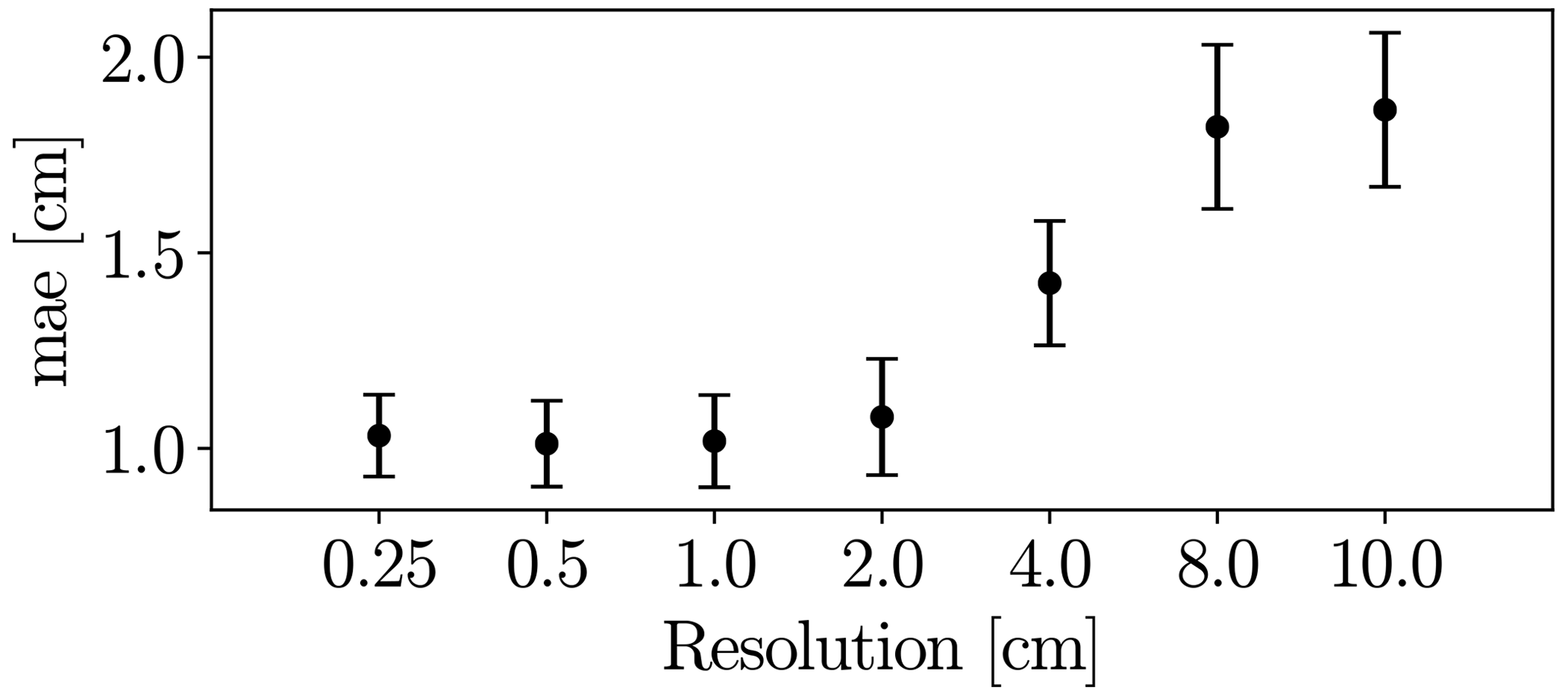
Figure 21Performance of GRAINet dm regression with different image resolutions (trained with MSE loss).
Interestingly, the performance for regressing dm with GRAINet drops only after downsampling with factor 16 (4 cm resolution) to a MAE of 1.4 cm and reaches a MAE of 1.9 cm at factor 40 (10 cm resolution) (Fig. 21). Corresponding dm scatter plots are shown in Fig. E2, where dispersion grows with coarser resolution. Avoiding the explicit detection of individual grains with the proposed regression approach has great potential and allows us to make reasonable predictions of dm even at lower image resolutions, as well as to adapt the resolution to the accuracy requirements of the application. In contrast to Carbonneau (2005), our GRAINet is able to predict mean diameters smaller than the ground sampling distance (Fig. E2), taking a big step towards grain size mapping beyond the image resolution. We believe that, in principle, GRAINet could even be used to process airborne imagery from countrywide flight campaigns, depending on the accuracy requirements of the application.
We have shown that GRAINet is able to estimate the full grain size distribution at particular locations in the orthophoto. Hence, we can derive the mean grading curve of entire gravel bars. The same architecture can also be trained to densely map the spatial distribution of the dm.
6.1 Manual component of the presented approach
Obviously, creating a large, manually labeled training dataset is time-consuming, which is a property our CNN shares with other supervised machine learning methods. However, at test time the proposed approach requires no parameter tuning by the user, which is a considerable advantage for large-scale applications, where traditional image processing pipelines struggle, since they are fairly sensitive to varying imaging conditions. Semiautomatic image labeling with the support of traditional image processing tools (Detert and Weitbrecht, 2012; Purinton and Bookhagen, 2019) might be an alternative way to speed up this annotation process. However, one would have to carefully avoid systematic algorithmic biases in the semiautomatic procedure, otherwise the CNN will almost certainly learn to faithfully reproduce those biases. Manual (re)labeling would still be required to prevent the CNN from replicating the systematic biases and failures of the rule-based system but could be limited to challenging samples. Similarly, systematic behaviors of specific annotators may also be learned by the model. Ideally, training data should thus be generated by different skilled annotators.
The CNN predictions for a full orthophoto are masked manually to the gravel bars. Our CNN is only trained on gravel images and did not see any purely non-gravel images patches with, e.g., vegetation, sand, or water. Consequently such inputs lie far outside the training distribution and result in arbitrary predictions that need to be masked out by the user. The network could also be trained to ignore samples with land cover other than gravel, but this is beyond the scope of the present paper. It could be added in the future to further reduce manual work.
6.2 Geographical generalization
We present experiments to evaluate the generalization of our approach to new locations, i.e., unseen gravel bars. In this setup, the data are exploited best, allowing the CNN to learn features invariant to the imaging conditions by providing 24 different training orthophotos in each experiment. That experimental setup is valid to investigate geographical generalization, since there is no strong correlation between bars from the same river. An alternative experiment would be to hold out all bars from a specific river for testing. This might be necessary in some geographical conditions with slowly varying river properties to avoid any misinterpretation and overly optimistic results. We have compared the average performance drop in the generalization experiment between five gravel bars on individual river reaches, i.e., bars that are separated by tributaries with new input of sediment, against all bars. Both groups yield comparable performance drops. We conclude that, within our dataset, seeing bars from the same river during training does not lead to over-optimistic results (see Fig. G1). Generalization is mainly affected by unique local environmental factors (e.g., wet stones, algae covering) that were not seen during training. Thus, in our case, we favor the former to maximize the number of training samples as well as the number of drone surveys with varying imaging conditions and local environmental factors.
The per bar generalization experiment is furthermore justified by the fact that the characteristics of the investigated gravel bars vary greatly along the same river, both quantitatively (mean dm, dm range in Table B1) and qualitatively (see Fig. F1 in Appendix F, where tiles are grouped by river name). Not only is this due to the distance between the bars but also due to the changing slope and the varying river bed widths in mountain environments (Reuss, Aare, Emme). Furthermore, the bars are geographically separated through tributaries (Aare, Rhone), leading to a drastic increase in the catchment areas between the bars. For example, at the river Rhone the catchment area is more than doubled from 982 km2 (at km 083.3) to 2485 km2 (at km 114.0). Additionally, the sediment transport is affected by dams at the rivers Aare, Rhone, and Reuss. Finally, the characteristics may also be artificially altered, as it is nowadays common in central Europe to replenish gravels of 2–3 cm to create spawning grounds for fish. For instance, the grain size distribution at the bar Reuss km 022.1 (and probably Reuss km 012.0) is very likely affected by such a targeted replenishment of sediment.
If we were to hold out, say, the whole river Aare, we would not only substantially reduce the number of training samples but also the diversity of imaging conditions. In fact, within our experimental setup we already present one hold-one-river-out experiment for the river Kleine Emme, from which only one bar is included in our dataset. Even though this bar contains the largest number of digital line samples, its estimated grain size distribution fits rather well in the geographical cross-validation experiment (see Fig. 18). The observed performance drop between the random and geographical cross-validation experiment for individual bars in Fig. 19 is rather explained by coarse gravel bars with a large mean dm and a wide dm range. Seeing bars from the same river during training and testing does not seem to have an effect (for instance, Aare).
Ultimately, it is important to keep in mind that data-driven approaches, like the one proposed, will only give reasonable estimates if the test data approximately match the training data distribution. These approaches will not perform well for out-of-distribution (OOD) samples. Detecting such OOD samples is an open problem and an active research direction.
6.3 Comparison to previous work
While existing statistical approaches are limited to output characteristic grain sizes (dm, d50), to the best of our knowledge GRAINet is the first data-driven approach that is able to regress a full, local grain size distribution at each location in an orthophoto. We are not aware of any previous work that evaluates grain size estimation over entire gravel bars in river beds or of a comparable study regarding geographical generalization.
Nevertheless, we present a generic learning approach; i.e., the same architecture can also be trained to directly predict other desired grain size metrics derived from the distribution, such as the mean diameter dm. Due to the end-to-end learning, our proposed CNN approach is able to extract global texture features that are informative about grain size beyond the image resolution and thus beyond the sensitivity of human photointerpretation or traditional image processing that relies on local image gradients to delineate individual grains. Even the latest work of Purinton and Bookhagen (2019) can only detect individual grains that have a b axis 20 times the ground sampling distance. Also, previous statistical approaches based on global image texture (Carbonneau et al., 2004) are limited by the input resolution and can only predict the median diameter d50 down to 3 cm at a comparable spatial resolution of 1 m. Hence, we believe that our approach advances the state of the art.
A direct quantitative comparison to previous work with different application focus and different data is only possible to a limited extent. For example, Buscombe (2013) evaluate on a mixed dataset with samples from rivers, natural beach, and continental shelf sediments and report normalized mean absolute errors of the estimated percentiles ranging from 10 to 29 %. In comparison, our dm regression yields a normalized mean absolute error of 18 %.
6.4 Advantages and limitations of the approach
Our CNN-based approach makes it possible to robustly estimate grain size distributions and characteristic mean diameters from raw images. By analyzing global image features, GRAINet avoids the explicit detection of individual grains, which makes the model more efficient and leads to a robust performance, even with lower image resolutions. The proposed approach enables the automatic analysis of entire gravel bars without destructive measures and with reasonable effort.
Advantages are manifold. First, results are objective and reproducible, as they are not influenced by a subjectively chosen sampling location and grain selection. Second, the resulting curves and dm represent the whole variability of grains of a gravel bar; thus, the disproportionately high effect of single coarse grains on the curve and on dm can be reduced. Consequently, the derived mean curves and its characteristic grain sizes can be considered representative.
Our experiments highlight some limitations due to the limited sample size for training. While 10-fold cross-fold validation yields very satisfying results, the poorer performance of the geographical cross-validation reveals that collecting and annotating sufficiently large and varied training sets is essential. Unseen unique local environmental factors such as wet stones or algae covering caused performance drops in the generalization experiment. However, if the model has seen a few of these samples (random cross-validation) the performance is more robust against such disturbances. Additionally, the performance of GRAINet deteriorates for very coarser gravel bars, as indicated by the error metrics of the distributions as well as for dm. The lower performance is caused by larger variability and by the high impact of individual, large grains, as well as by the unbalanced data distribution (only 14 % of the digital line samples have a dm>10 cm). Application of GRAINet, trained with our dataset, is thus not always satisfactory for coarse, unseen gravel bars. In order to improve results and extend potential applications fields, further digital line samples from additional UAV surveys should be collected.
Finally, the best performance has been achieved with high-resolution imagery taken at 10 m flying altitude. At this altitude it takes approximately 15 min to cover an area of 1 ha with a DJI Phantom 4 Pro (that has a max flight time of approx. 30 min per battery). It would be advantageous to reduce the flight time per area by flying at higher altitudes. As our resolution study on artificially downsampled images shows, the CNN may yield satisfactory performance on images with 1–2 cm resolution corresponding to 40–80 m flying altitude. While this is a promising result, it remains to be tested on images taken at such flying altitudes. We expect that retraining the model with high altitude image–label pairs will lead to similar performance as in the artificial case.
6.5 Potential applications
The presented GRAINet method can be applied to all rivers that fulfill the following conditions: dry gravel bars (meaning low water conditions, as grains in deeper water cannot be analyzed) and no obstacles in the flight area (especially trees along the rivers can cause occlusions). Despite these limitations, we are convinced that our results confirm the large potential of UAV surveys in combination with CNNs for grain size analysis. There are several applications which become possible with GRAINet in a quality that was hitherto not achievable. Perhaps the greatest asset is the creation of dense, spatially explicit, georeferenced maps of dm. Not only can they help to understand spatial sorting effects of bed-load transport processes but they can also be used to calibrate two- or even three-dimensional fractional transport models. In addition, the variability of dm within a gravel bar can provide important information regarding the bed-load regime and the ecological value of the river (e.g., as aquatic habitat). For example, a lack of variability in the finer grain sizes is a clear sign for bed armoring and thus an important indicator for a bed-load deficit. Consequently, the maps of dm are ideal for large-scale monitoring in space and time, since they open up the possibility to study entire bars or river branches at virtually no additional cost. Our automatic approach handles all samples consistently and allows for unbiased monitoring over long times, as there is no variation due to changing operators (Wohl et al., 1996). Furthermore, the ability to estimate mean diameters from lower image resolutions (up to 2 cm ground sampling distance) will allow us to cover even larger regions flying the UAV at higher altitudes. Due to the high resolution of the resulting maps and distribution estimates, local effects on bars can be investigated. Ultimately, this could allow hydrologists to explore new research directions that advance the understanding of fluvial geomorphology. While spatially explicit data may lead to an improved calibration of numerical models, we may gain new insights into how spatial heterogeneity affects the sediment transport capacity as well as the aquatic biodiversity.
We have presented GRAINet, a data-driven approach centered on deep learning to analyze grain size distributions from georeferenced UAV images with a convolutional neural network. In an experimental evaluation with 1491 digital line samples, the method achieves an accuracy that makes it relevant for several practical applications. The new possibility to carry out holistic analyses of entire gravel bars overcomes the limitations of sparse field sampling approaches (e.g., line sampling by Fehr, 1987), which is cumbersome and prone to subjective biases.
As CNNs are generic machine learning models, they offer great flexibility to directly predict other variables, like, for example, the ratio or other specific percentiles (Buscombe, 2019). In fact, it might be promising to design a multi-task approach, in order to exploit the correlations and synergies between different variables and parametrizations describing the same grain size distribution. Obviously, collecting more training data can be expected to benefit the generalization performance of GRAINet. Data annotation could potentially be supported with active learning (e.g., Settles, 2009), where the model is gradually updated and intermediate predictions guide the selection of the most informative samples that should be labeled to further improve the model. Another technically interesting direction to explore is domain adaptation, in order to exploit unlabeled image data as a source of information and improve the generalization to a new domain with potentially different characteristics (i.e., new gravel bars).
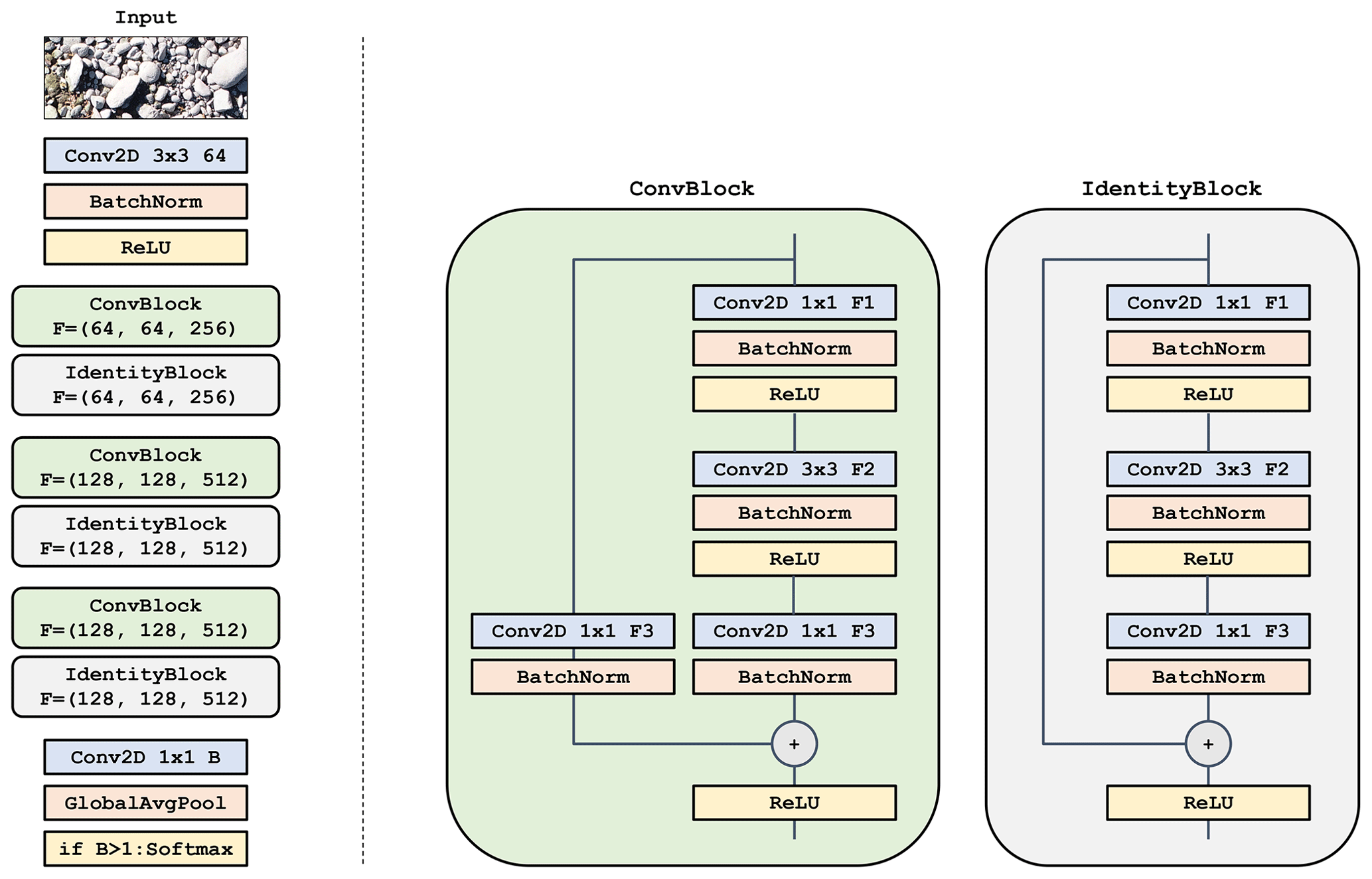
Figure A1Illustration of the convolutional neural network architecture. Left: full architecture where denotes the number of filters of the three convolutional layers within the residual blocks. The number of outputs B corresponds to the estimated histogram bins. To estimate a scalar (e.g., mean diameter) this B can be set to one. Right: the respective residual blocks. The ConvBlock has a learnable skip connection and is used when the number of output features is not equal to the number of input features. If constant, the IdentityBlock forwards the input.
Table B1Overview of the 25 investigated gravel bars. From left to right: slope and bed width of the river at this location with the corresponding annual mean water runoff. Number of annotated image tiles (digital line samples). Ground truth statistics of the characteristic mean diameter dm.
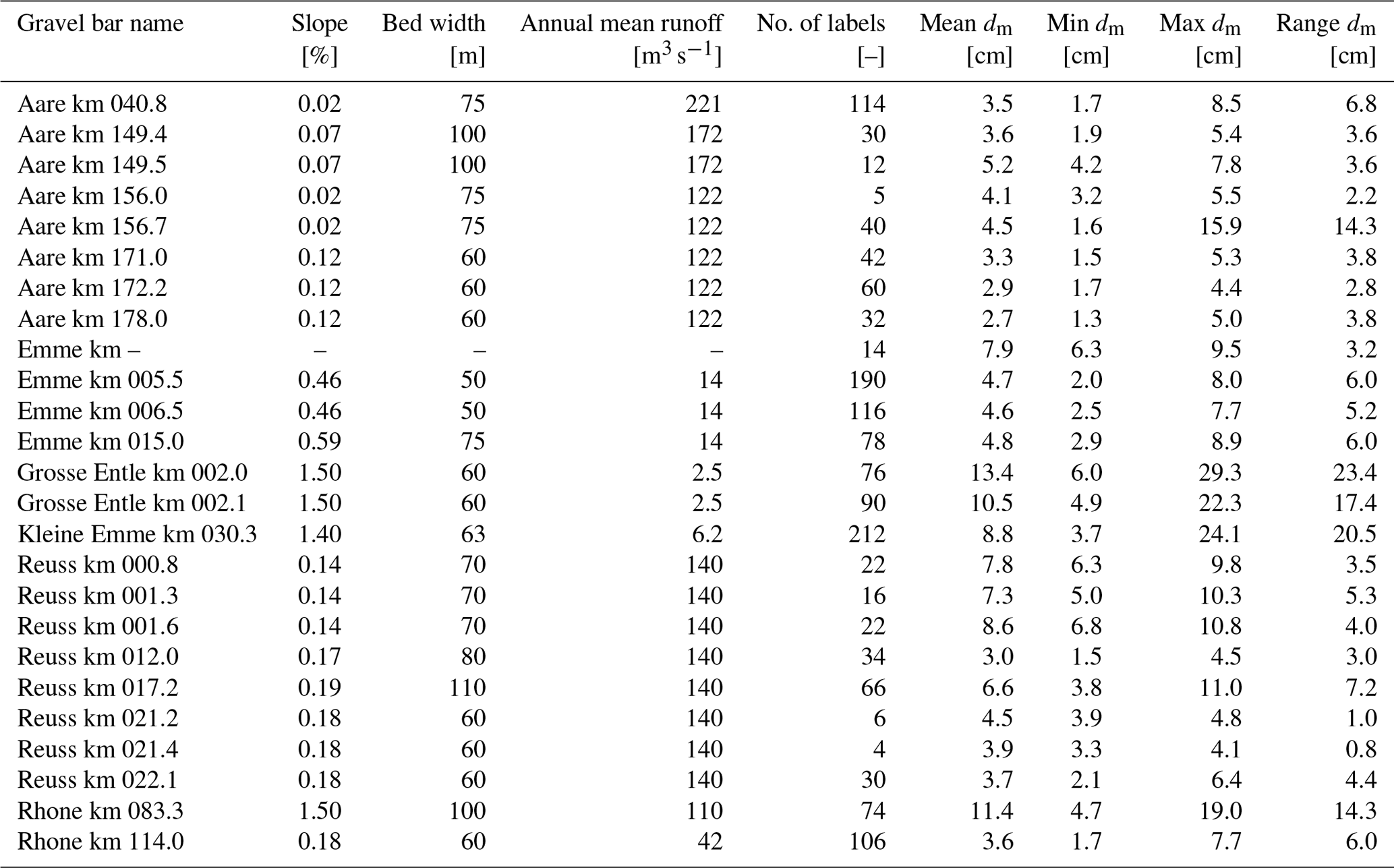
Table C1Statistics of the mean diameter dm [cm] from three to five human annotations for 17 randomly selected image tiles.

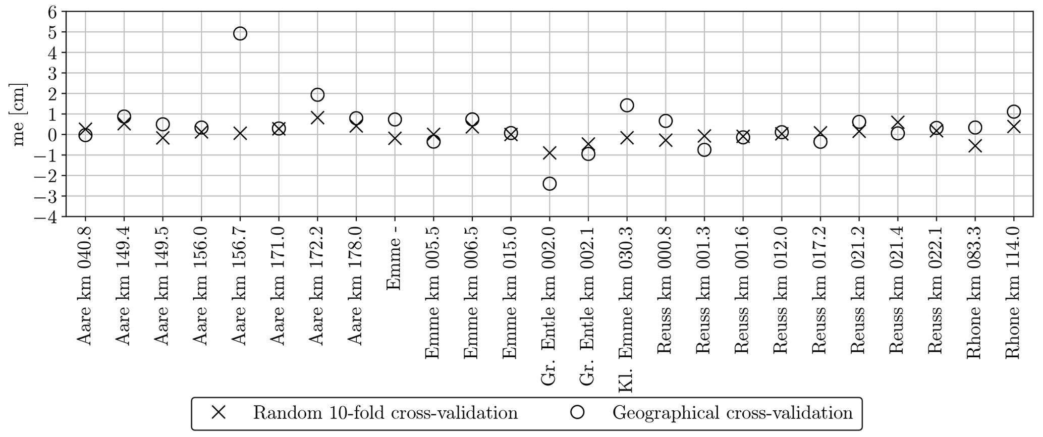
Figure D1Mean error (bias) of the GRAINet end-to-end dm regression per gravel bar (random and geographical cross-validation). A positive error implies that the GRAINet prediction was higher than the ground truth.
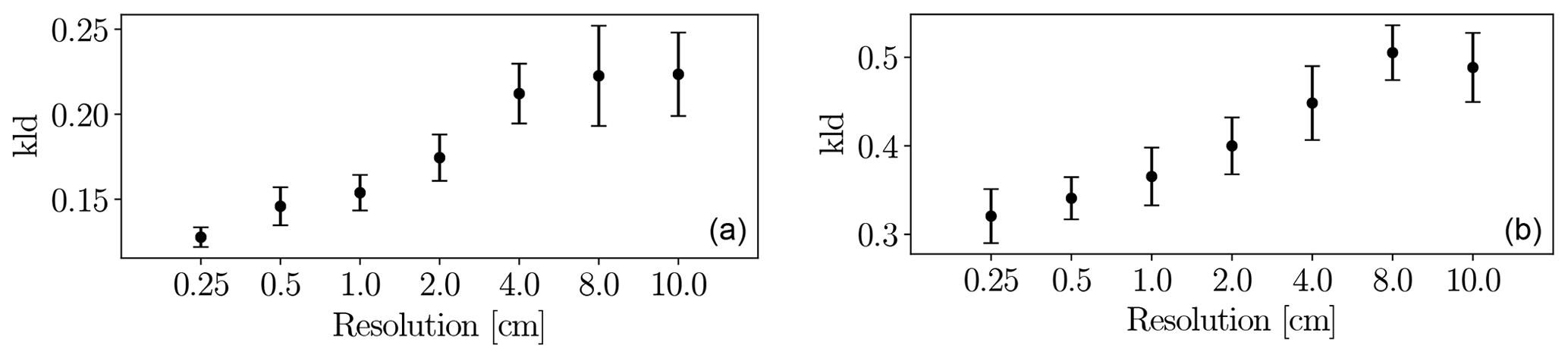
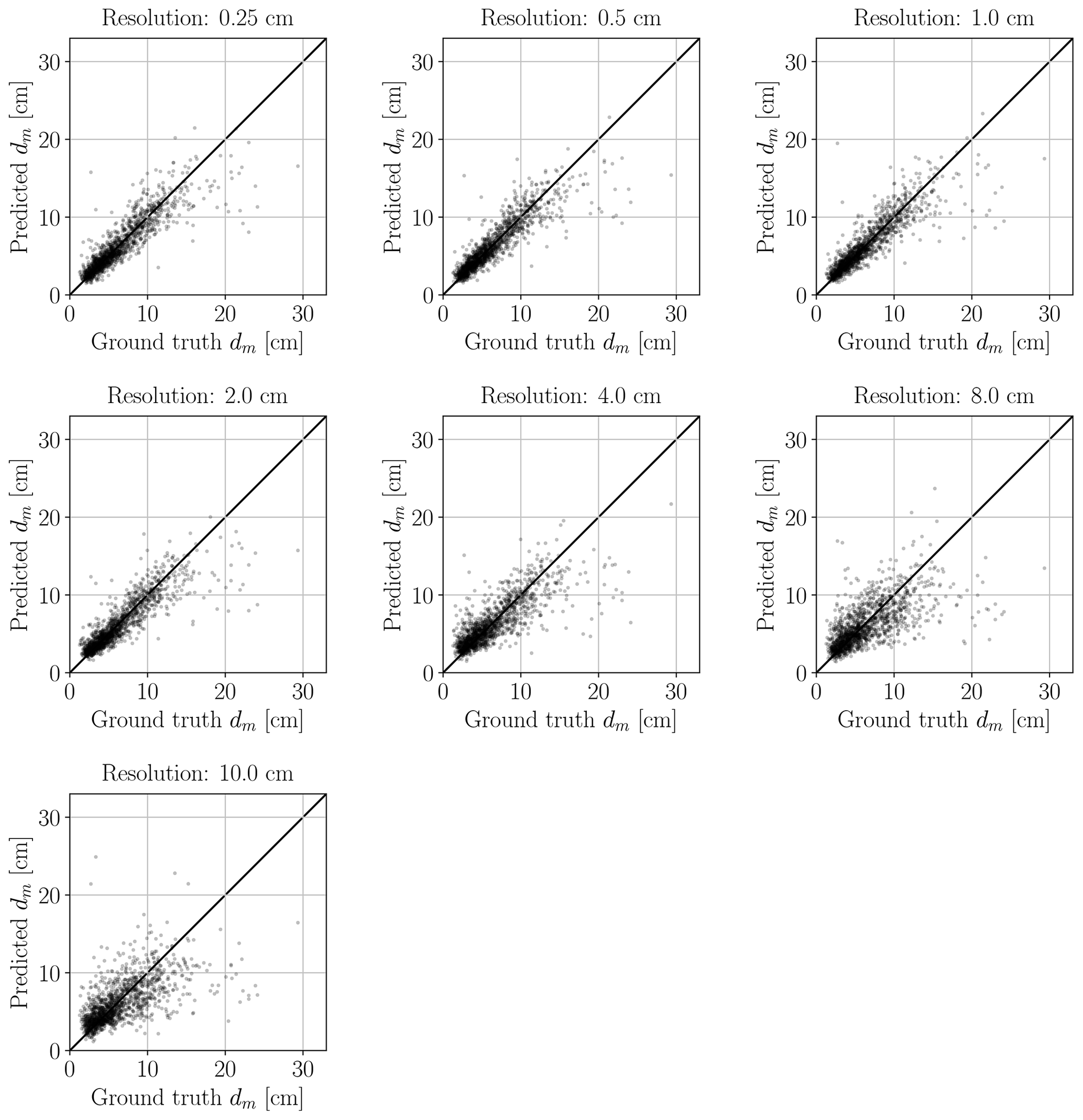
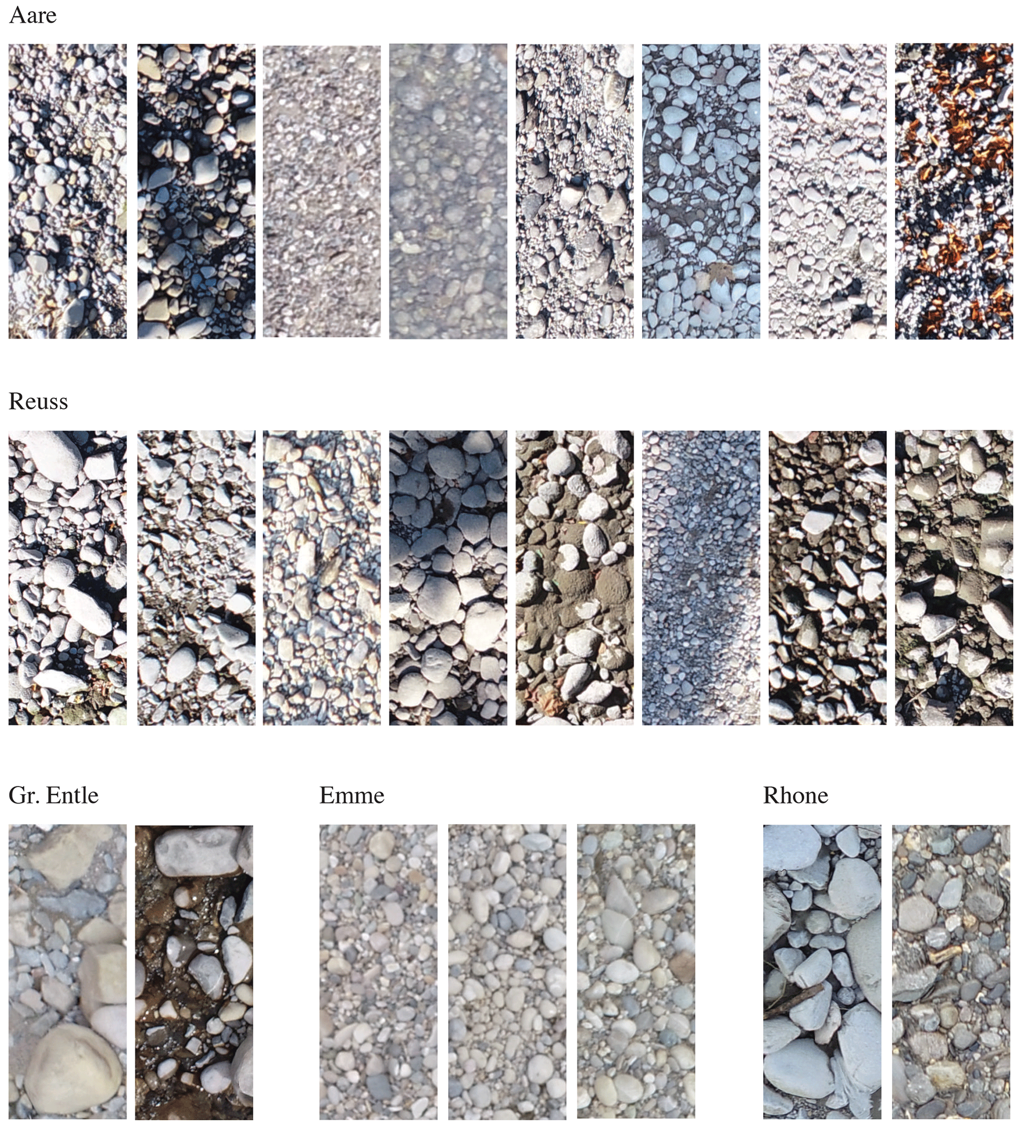
Figure F1Tiles grouped by river name. The examples illustrate the variability between different bars along the same river.
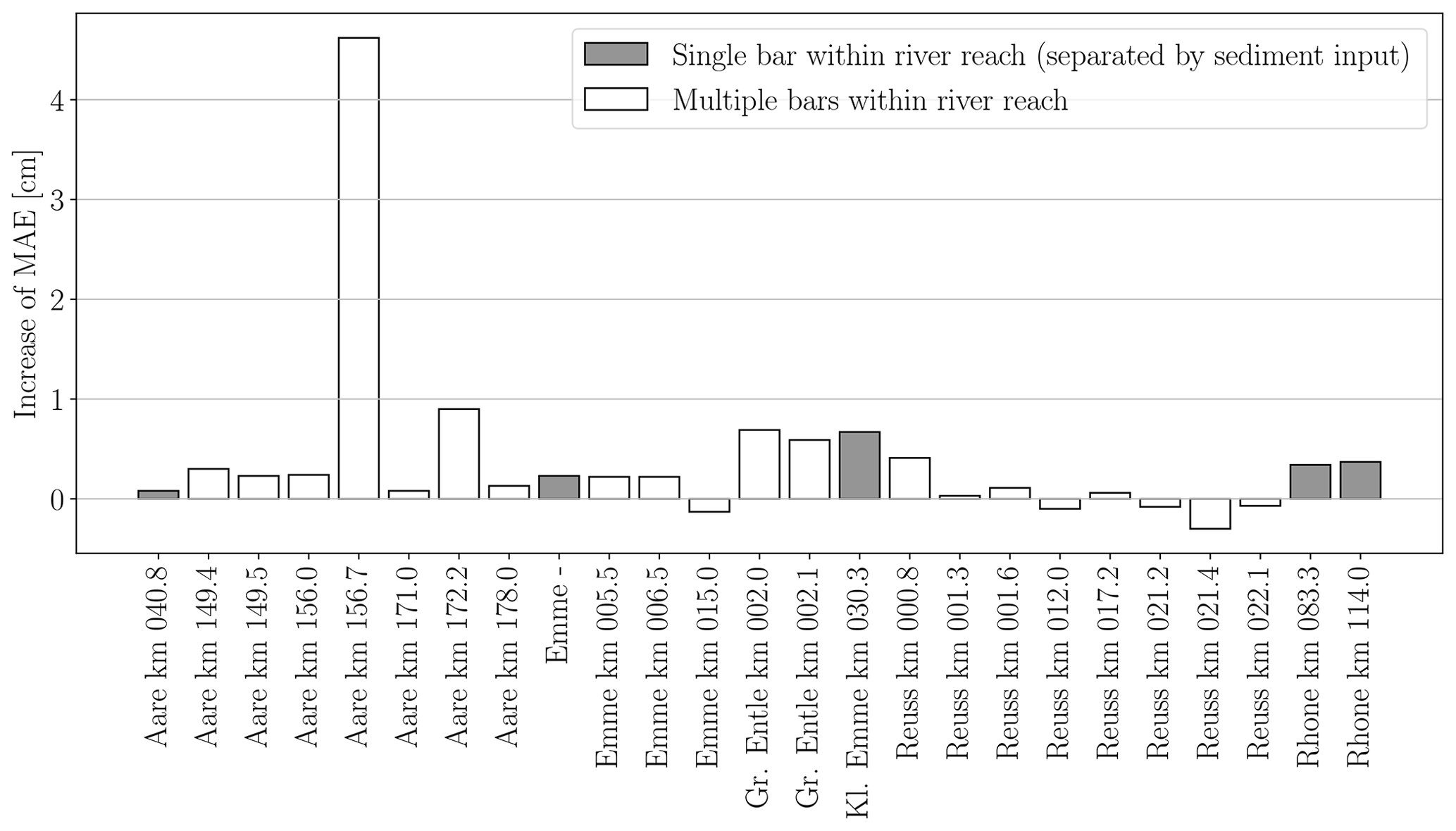
Figure G1Generalization performance per gravel bar. Increase of mean absolute error (MAE) from the random cross-validation to the geographical generalization experiment for the GRAINet end-to-end dm regression. A positive value means that the generalization experiment has a higher error. Gravel bars on individual river reaches (i.e., separated by tributaries) are depicted in gray.
The code with a demonstration on a subset of the data is available: https://github.com/langnico/GRAINet (last access: May 2021). Due to licensing restrictions, the complete dataset (Irniger and Hunziker, 2020) may only be used for research purposes and can be requested by contacting andrea.irniger@hzp.ch.
NL and AR developed the code and carried out the experiments. AI designed the data acquisition and analyzed the results. KS, JW, and RH provided guidance during project planning and experimentation. All authors contributed to the article, under the lead of NL and AI.
The authors declare that they have no conflict of interest.
We thank Hunziker, Zarn & Partner for sharing the ground truth data for this research project.
This paper was edited by Matjaz Mikos and reviewed by Patrice Carbonneau and two anonymous referees.
Adams, J.: Gravel size analysis from photographs, J. Hydr. Eng. Div.-ASCE, 105, 1247–1255, 1979. a
Babej, J., Máčka, Z., Ondrejka, P., and Peterová, P.: Surface grain size variation within gravel bars: a case study of the River Opava, Czech Republic, Geogr. Fis. Dinam. Quatern., 39, 3–12, 2016. a
Badoux, A., Andres, N., and Turowski, J. M.: Damage costs due to bedload transport processes in Switzerland, Nat. Hazards Earth Syst. Sci., 14, 279–294, https://doi.org/10.5194/nhess-14-279-2014, 2014. a
Black, M., Carbonneau, P., Church, M., and Warburton, J.: Mapping sub-pixel fluvial grain sizes with hyperspatial imagery, Sedimentology, 61, 691–711, 2014. a, b
Brasington, J., Vericat, D., and Rychkov, I.: Modeling river bed morphology, roughness, and surface sedimentology using high resolution terrestrial laser scanning, Water Resour. Res., 48, W11519, https://doi.org/10.1029/2012WR012223, 2012. a
Bunte, K. and Abt, S. R.: Sampling surface and subsurface particle-size distributions in wadable gravel-and cobble-bed streams for analyses in sediment transport, hydraulics, and streambed monitoring, US Department of Agriculture, Forest Service, Rocky Mountain Research Station, 2001. a, b, c, d, e, f, g, h, i
Buscombe, D.: Transferable wavelet method for grain-size distribution from images of sediment surfaces and thin sections, and other natural granular patterns, Sedimentology, 60, 1709–1732, 2013. a, b, c, d, e
Buscombe, D.: SediNet: A configurable deep learning model for mixed qualitative and quantitative optical granulometry, Earth Surf. Proc. Land., 5, 638–651, https://doi.org/10.1002/esp.4760, 2019. a, b, c, d, e
Buscombe, D. and Masselink, G.: Grain-size information from the statistical properties of digital images of sediment, Sedimentology, 56, 421–438, 2009. a
Buscombe, D., Rubin, D., and Warrick, J.: A universal approximation of grain size from images of noncohesive sediment, J. Geophys. Res.-Earth, 115, F02015, https://doi.org/10.1029/2009JF001477, 2010. a
Butler, J. B., Lane, S. N., and Chandler, J. H.: Automated extraction of grain-size data from gravel surfaces using digital image processing, J. Hydraul. Res., 39, 519–529, 2001. a, b
Carbonneau, P. E.: The threshold effect of image resolution on image-based automated grain size mapping in fluvial environments, Earth Surf. Proc. Land., 30, 1687–1693, 2005. a
Carbonneau, P. E., Lane, S. N., and Bergeron, N. E.: Catchment-scale mapping of surface grain size in gravel bed rivers using airborne digital imagery, Water Resour. Res., 40, W07202, https://doi.org/10.1029/2003WR002759, 2004. a, b, c
Carbonneau, P. E., Bergeron, N., and Lane, S. N.: Automated grain size measurements from airborne remote sensing for long profile measurements of fluvial grain sizes, Water Resour. Res., 41, W11426, https://doi.org/10.1029/2005WR003994, 2005. a, b
Carbonneau, P., Bizzi, S., and Marchetti, G.: Robotic photosieving from low-cost multirotor sUAS: a proof-of-concept, Earth Surf. Proc. Land., 43, 1160–1166, 2018. a, b, c, d
de Haas, T., Ventra, D., Carbonneau, P. E., and Kleinhans, M. G.: Debris-flow dominance of alluvial fans masked by runoff reworking and weathering, Geomorphology, 217, 165–181, 2014. a
Detert, M. and Weitbrecht, V.: Automatic object detection to analyze the geometry of gravel grains – A free stand-alone tool, River Flow 2012 – Proceedings of the International Conference on Fluvial Hydraulics, Taylor & Francis Group, London, 595–600, 2012. a, b, c, d, e, f
Fehr, R.: Einfache Bestimmung der Korngrössenverteilung von Geschiebematerial mit Hilfe der Linienzahlanalyse [Simple detection of grain size distribution of sediment material using line-count analysis], in German, Schweizer Ingenieur und Architekt, 105, 1104–1109, 1987. a, b, c, d, e, f, g, h, i
Graham, D. J., Reid, I., and Rice, S. P.: Automated sizing of coarse-grained sediments: image-processing procedures, Math. Geol., 37, 1–28, 2005. a, b
Graham, D. J., Rollet, A.-J., Piégay, H., and Rice, S. P.: Maximizing the accuracy of image-based surface sediment sampling techniques, Water Resour. Res., 46, W02508, https://doi.org/10.1029/2008WR006940, 2010. a
Gregory, K. J.: Human influence on the morphological adjustment of river channels: The evolution of pertinent concepts in river science, River Res. Appl., 35, 1097–1106, 2019. a
Grill, G., Lehner, B., Thieme, M., Geenen, B., Tickner, D., Antonelli, F., Babu, S., Borrelli, P., Cheng, L., Crochetiere, H., Ehalt Macedo, H., Filgueiras, R., Goichot, M., Higgins, J., Hogan, Z., Lip, B., McClain, M. E., Meng, J., Mulligan, M., Nilsson, C., Olden, J. D., Opperman, J. J., Petry, P., Reidy Liermann, C., Sáenz, L., Salinas-Rodríguez, S., Schelle, P., Schmitt, R. J. P., Snider, J., Tan, F., Tockner, K., Valdujo, P. H., van Soesbergen, A., and Zarfl, C.: Mapping the world's free-flowing rivers, Nature, 569, 215–221, 2019. a
Habersack, H., Hengl, M., Huber, B., Lalk, P., Tritthart, M., Habersack, H., Hengl, M., Huber, B., Lalk, P., and Tritthart, M.: Fließgewässermodellierung – Arbeitsbehelf Feststofftransport und Gewässermorphologie [River modelling–working aid for sediment transport and fluvial morphology], Austrian Federal Ministry of Agriculture, Forestry, Environment and Water Management and Österreichischer Wasser-und Abfallwirtschaftsverband ÖWAV, Vienna, 2011. a, b, c
He, K., Zhang, X., Ren, S., and Sun, J.: Deep residual learning for image recognition, in: Proceedings of the IEEE conference on computer vision and pattern recognition, 770–778, 2016. a
He, K., Gkioxari, G., Dollár, P., and Girshick, R.: Mask r-cnn, in: Proceedings of the IEEE international conference on computer vision, 2961–2969, 2017. a
Huang, G.-H., Atkinson, P. M., and Wang, C.-K.: Quantifying the scales of spatial variation in gravel beds using terrestrial and airborne laser scanning data, Open Geosci., 10, 607–617, 2018. a
Ibbeken, H. and Schleyer, R.: Photo-sieving: A method for grain-size analysis of coarse-grained, unconsolidated bedding surfaces, Earth Surf. Proc. Land., 11, 59–77, 1986. a
Ioffe, S. and Szegedy, C.: Batch normalization: Accelerating deep network training by reducing internal covariate shift, arXiv: preprint, arXiv:1502.03167, 2015. a
Irniger, A. and Hunziker, R.: UAV grain size dataset for Swiss rivers created by Hunziker, Zarn & Partner used to develop GRAINet, The data may be requested for research purposes, 2020. a, b
Kingma, D. P. and Ba, J.: Adam: A method for stochastic optimization, arXiv: preprint, arXiv:1412.6980, 2014. a
Krumbein, W. C. and Pettijohn, F. J.: Manual of Sedimentary Petrography. XIV + 549 pp., 8:o, 265 fig. New York and London 1938, (1939). D. Appleton – Century Company. 8 6.50 (30 s.), Geologiska Föreningen i Stockholm Förhandlingar, 61, 225–227, https://doi.org/10.1080/11035893909452786, 1938. a
LeCun, Y. A., Bottou, L., Orr, G. B., and Müller, K.-R.: Efficient backprop, in: Neural networks: Tricks of the trade, Springer, 9–48, 2012. a
Meyer-Peter, E. and Müller, R.: Formulas for bed-load transport, in: IAHSR 2nd meeting, Stockholm, appendix 2, IAHR, 1948. a
Nelson, J. M., McDonald, R. R., Shimizu, Y., Kimura, I., Nabi, M., and Asahi, K.: Modelling flow, sediment transport and morphodynamics in rivers, Tools in fluvial geomorphology, Wiley, 412–441, https://doi.org/10.1002/9781118648551.ch18, 2016. a
Piégay, H., Arnaud, F., Belletti, B., Bertrand, M., Bizzi, S., Carbonneau, P., Dufour, S., Liebault, F., Ruiz-Villanueva, V., and Slater, L.: Remotely Sensed Rivers in the Anthropocene: State of the Art and Prospects, Earth Surf. Proc. Land., 45, 157–188, https://doi.org/10.1002/esp.4787, 2019. a
Poeppl, R. E., Keesstra, S. D., and Maroulis, J.: A conceptual connectivity framework for understanding geomorphic change in human-impacted fluvial systems, Geomorphology, 277, 237–250, 2017. a
Purinton, B. and Bookhagen, B.: Introducing PebbleCounts: a grain-sizing tool for photo surveys of dynamic gravel-bed rivers., Earth Surf. Dynam., 7, 859–877, https://doi.org/10.5194/esurf-7-859-2019, 2019. a, b, c, d, e
Ramdas, A., Trillos, N. G., and Cuturi, M.: On wasserstein two-sample testing and related families of nonparametric tests, Entropy, 19, 47, https://doi.org/10.3390/e19020047, 2017. a
Rice, S. and Church, M.: Grain size along two gravel-bed rivers: statistical variation, spatial pattern and sedimentary links, Earth Surf. Proc. Land., 23, 345–363, 1998. a
Rice, S. P. and Church, M.: Grain-size sorting within river bars in relation to downstream fining along a wandering channel, Sedimentology, 57, 232–251, 2010. a
Rubin, D. M.: A simple autocorrelation algorithm for determining grain size from digital images of sediment, J. Sediment. Res., 74, 160–165, 2004. a, b
Settles, B.: Active learning literature survey, Tech. Rep., University of Wisconsin–Madison, Department of Computer Sciences, available at: http://digital.library.wisc.edu/1793/60660 (last access: May 2021), 2009. a
Sharma, K., Gold, M., Zurbruegg, C., Leal-Taixé, L., and Wegner, J. D.: HistoNet: Predicting size histograms of object instances, in: The IEEE Winter Conference on Applications of Computer Vision, 3637–3645, 2020. a, b, c
Shen, C., Laloy, E., Elshorbagy, A., Albert, A., Bales, J., Chang, F.-J., Ganguly, S., Hsu, K.-L., Kifer, D., Fang, Z., Fang, K., Li, D., Li, X., and Tsai, W.-P.: HESS Opinions: Incubating deep-learning-powered hydrologic science advances as a community, Hydrol. Earth Syst. Sci., 22, 5639–5656, https://doi.org/10.5194/hess-22-5639-2018, 2018. a, b
Sime, L. and Ferguson, R.: Information on grain sizes in gravel-bed rivers by automated image analysis, J. Sediment. Res., 73, 630–636, 2003. a
Simon, A. and Rinaldi, M.: Disturbance, stream incision, and channel evolution: The roles of excess transport capacity and boundary materials in controlling channel response, Geomorphology, 79, 361–383, 2006. a
Spada, D., Molinari, P., Bertoldi, W., Vitti, A., and Zolezzi, G.: Multi-Temporal Image Analysis for Fluvial Morphological Characterization with Application to Albanian Rivers, ISPRS Int. J. Geo.-Inf. 7, 314, 2018. a
Surian, N.: Downstream variation in grain size along an Alpine river: analysis of controls and processes, Geomorphology, 43, 137–149, 2002. a, b
Surian, N. and Rinaldi, M.: Morphological response to river engineering and management in alluvial channels in Italy, Geomorphology, 50, 307–326, 2003. a
Van Horn, G., Branson, S., Farrell, R., Haber, S., Barry, J., Ipeirotis, P., Perona, P., and Belongie, S.: Building a bird recognition app and large scale dataset with citizen scientists: The fine print in fine-grained dataset collection, in: Proceedings of the IEEE Conference on Computer Vision and Pattern Recognition, 595–604, 2015. a, b
Vázquez-Tarr'io, D., Borgniet, L., Liébault, F., and Recking, A.: Using UAS optical imagery and SfM photogrammetry to characterize the surface grain size of gravel bars in a braided river (Vénéon River, French Alps), Geomorphology, 285, 94–105, 2017. a
Verdú, J. M., Batalla, R. J., and Martínez-Casasnovas, J. A.: High-resolution grain-size characterisation of gravel bars using imagery analysis and geo-statistics, Geomorphology, 72, 73–93, 2005. a, b
Wohl, E. E., Anthony, D. J., Madsen, S. W., and Thompson, D. M.: A comparison of surface sampling methods for coarse fluvial sediments, Water Resour. Res., 32, 3219–3226, 1996. a, b, c, d
Wolman, M. G.: A method of sampling coarse river-bed material, EOS T. Am. Geophys. Un., 35, 951–956, 1954. a
Woodget, A., Fyffe, C., and Carbonneau, P.: From manned to unmanned aircraft: Adapting airborne particle size mapping methodologies to the characteristics of sUAS and SfM, Earth Surf. Proc. Land., 43, 857–870, 2018. a, b
Wu, F.-C., Wang, C.-K., and Huang, G.-H.: Delineation of gravel-bed clusters via factorial kriging, Geomorphology, 308, 161–174, 2018. a
Zettler-Mann, A. and Fonstad, M.: Riverscape mapping and hyperscale analysis of the sediment links concept, Geomorphology, 350, 106920, https://doi.org/10.1016/j.geomorph.2019.106920, 2020. a
To the best of our knowledge, this includes at least the following German-speaking countries: Switzerland, Germany, and Austria.
It is worth noting that the annotation strategy and the CNN are not tightly coupled. Since the CNN is agnostic, it could be trained on grain size data created with different sampling strategies to meet other national standards.
While not clearly explained in Buscombe (2019), the results seem to suffer from overfitting, due to a flaw in the experimental setup. Our review of the published source code revealed that the stopping criterion for the training uses the test data, leading to overly optimistic numbers.
With the exception of location Emme –, which is a gravel pile outside the channel.
https://www.dji.com/ch/phantom-4-pro (last access: 23 March 2020)
https://www.pix4d.com/de/produkt/pix4dcapture (last access: 4 April 2020)
https://www.agisoft.com/ (last access: 4 April 2020)
In contrast to Sharma et al. (2020), we estimate relative instead of absolute distributions. While they show that the L1 loss and the KL divergence can be combined to capture scale and shape of the distribution, respectively, we simply fix the scale of the predicted distribution with a softmax before the output.
For completeness, we note that there is a smoothed and symmetric (but less popular) variant of KLD, i.e., the Jensen–Shannon divergence.
- Abstract
- Introduction
- Related work
- Data
- Method
- Experimental results
- Discussion
- Conclusions and future work
- Appendix A: CNN architecture illustration
- Appendix B: Overview of investigated gravel bars
- Appendix C: Repeated human annotation
- Appendix D: Generalization across gravel bars
- Appendix E: Resolution study
- Appendix F: Tiles grouped by river name
- Appendix G: Generalization performance per gravel bar
- Code and data availability
- Author contributions
- Competing interests
- Acknowledgements
- Review statement
- References