Global ecosystem-scale plant hydraulic traits retrieved using model–data fusion

Droughts are expected to become more frequent and severe under climate change, increasing the need for accurate predictions of plant drought response. This response varies substantially, depending on plant properties that regulate water transport and storage within plants, i.e., plant hydraulic traits. It is, therefore, crucial to map plant hydraulic traits at a large scale to better assess drought impacts. Improved understanding of global variations in plant hydraulic traits is also needed for parameterizing the latest generation of land surface models, many of which explicitly simulate plant hydraulic processes for the first time. Here, we use a model–data fusion approach to evaluate the spatial pattern of plant hydraulic traits across the globe. This approach integrates a plant hydraulic model with data sets derived from microwave remote sensing that inform ecosystem-scale plant water regulation. In particular, we use both surface soil moisture and vegetation optical depth (VOD) derived from the X-band Japan Aerospace Exploration Agency (JAXA) Advanced Microwave Scanning Radiometer for Earth Observing System (EOS; collectively AMSR-E). VOD is proportional to vegetation water content and, therefore, closely related to leaf water potential. In addition, evapotranspiration (ET) from the Atmosphere–Land Exchange Inverse (ALEXI) model is also used as a constraint to derive plant hydraulic traits. The derived traits are compared to independent data sources based on ground measurements. Using the K-means clustering method, we build six hydraulic functional types (HFTs) with distinct trait combinations – mathematically tractable alternatives to the common approach of assigning plant hydraulic values based on plant functional types. Using traits averaged by HFTs rather than by plant functional types (PFTs) improves VOD and ET estimation accuracies in the majority of areas across the globe. The use of HFTs and/or plant hydraulic traits derived from model–data fusion in this study will contribute to improved parameterization of plant hydraulics in large-scale models and the prediction of ecosystem drought response.

1 Introduction

Water stress during drought restricts photosynthesis, thus weakening the strength of the terrestrial carbon sink (Ma et al., 2012; Wolf et al., 2016; Konings et al., 2017) and possibly causing plant mortality under severe conditions (McDowell et al., 2016; Adams et al., 2017; Choat et al., 2018). The plant response to water stress also directly controls regional water resources and drought propagation by modulating water flux and energy partitioning between the land surface and the atmosphere (Goulden and Bales, 2014; Manoli et al., 2016; Anderegg et al., 2019). However, how plants regulate water, carbon, and energy fluxes and plant mortality under drought could vary considerably depending on plant properties, particularly plant hydraulic traits (Sack et al., 2016; Hartmann et al., 2018; McDowell et al., 2019). Understanding this variation is therefore crucial for the accurate prediction of ecosystem dynamics under changing climate.

Plant hydraulic traits at both stem (e.g., ψ_50,x; the xylem water potential under 50 % loss of xylem conductivity) and stomatal (e.g, g₁; the sensitivity parameter of stomatal conductance to vapor pressure deficit) levels control plant water uptake and the extent of stomatal closure under water stress (Martin-StPaul et al., 2017; Feng et al., 2017; Meinzer et al., 2017; Anderegg et al., 2017). Distinct hydraulic traits across species and plant communities define hydraulic strategies, which lead to different responses of leaf water potential and gas exchange during drought (Matheny et al., 2017; Barros et al., 2019). Plant hydraulic traits play critical roles in predicting stomatal response to stress (Sperry et al., 2017; Liu et al., 2020a), plant water storage (Huang et al., 2017), leaf desiccation (Blackman et al., 2019), and drought-driven tree mortality risk (Anderegg et al., 2016; Powell et al., 2017; Liu et al., 2017; De Kauwe et al., 2020). As a result of their effect on the surface energy balance, plant hydraulic traits also impact the magnitude of land–atmosphere feedbacks (Anderegg et al., 2019). In dry tropical forests, leaf water potential – which is directly influenced by hydraulic traits – has also been shown to affect leaf phenology (Xu et al., 2016). As a result, it has been increasingly recognized that plant hydraulic traits are important for mediating ecosystem drought response and hydroclimatic feedbacks at regional to global scales (Choat et al., 2012; Anderegg, 2015; Choat et al., 2018; Hartmann et al., 2018).

Understanding how plant hydraulic traits modulate large-scale drought responses requires mapping these traits. At large scales, plant traits are often parameterized based on plant functional types (PFTs), such as evergreen needleleaf forests, evergreen broadleaf forests, deciduous broadleaf forests, mixed forests, shrublands, grasslands, and croplands. However, plant hydraulic traits can vary as much across PFTs as within them (Anderegg, 2015; Konings and Gentine, 2017). Finding alternative ways to scale up in situ measurements using a bottom-up approach is challenging because the spatial coverage of such measurements is often limited and biased towards temperate regions. Furthermore, plant hydraulic traits are highly variable within species (Anderegg, 2015) and even between different components of a single plant and across vertical gradients within individual trees (Johnson et al., 2016). Alternatively, because microwave remote sensing observations of vegetation optical depth (VOD) are sensitive to leaf water potential (Momen et al., 2017; Konings et al., 2019; Holtzman et al., 2021), they may carry implicit information that can be used to disentangle plant hydraulic traits, without the need for explicit upscaling.

Konings and Gentine (2017) first derived plant hydraulic trait variations at large scales by using VOD to calculate the effective ecosystem-scale isohydricity. The isohydricity reflects the response of leaf water potential as soil water potential dries down (Tardieu and Simonneau, 1998). At a stand scale, this plant physiological metric has been used to explain photosynthesis variations (Roman et al., 2015) and drought mortality risk (McDowell et al., 2008) across species. At a global scale, remote-sensing-derived isohydricity patterns have been used to explain photosynthesis sensitivity to vapor pressure deficit and soil moisture in North American grasslands (Konings et al., 2017) and the Amazon (Giardina et al., 2018), to explore the interannual variability in isohydricity (Wu et al., 2020) and to explain the relationship between drought resistance and resilience in gymnosperms (Li et al., 2020). However, because isohydricity is an emergent rather than intrinsic property, it is subject to change with environmental conditions (Hochberg et al., 2018; Novick et al., 2019; Feng et al., 2019; Mrad et al., 2019). Furthermore, isohydricity is influenced by both stomatal and xylem traits (Martínez-Vilalta et al., 2014), which do not always co-vary (Manzoni et al., 2013; Martínez-Vilalta et al., 2014; Bartlett et al., 2016; Martínez-Vilalta and Garcia-Forner, 2017). Estimating intrinsic xylem and stomatal traits separately is, therefore, necessary for better assessment of plant drought response.

From a modeling perspective, as plant hydraulics has been increasingly recognized as a central link connecting hydroclimatic processes and ecosystem ecology (Sack et al., 2016; McDowell et al., 2019), land surface and dynamic vegetation models that explicitly incorporate plant hydraulics are becoming more common (e.g., Xu et al., 2016; Christoffersen et al., 2016; Kennedy et al., 2019; De Kauwe et al., 2020; Eller et al., 2020). However, explicit plant hydraulic representation also requires parameterization choices for the associated plant hydraulic traits. As discussed above, a bottom-up scaling of in situ measurements is likely to miss significant fractions of the spatial variability in these parameters. Alternatively, Liu et al. (2020a) took a top-down inversion approach by integrating a plant hydraulic model with ET data observed at FLUXNET sites. This model–data fusion approach identifies the most likely traits generating modeled dynamics consistent with observations, thus providing effective hydraulic traits that represent ecosystem-scale behaviors. Similar model–data fusion approaches have been previously applied in carbon cycle models (e.g. Wang et al., 2009; Dietze et al., 2013; Quetin et al., 2020). Not surprisingly, many of these applications suggest that integrating informative observations is among the keys to effectively constraining model parameters.

Here, we use the model–data fusion approach to evaluate the global pattern of ecosystem-scale plant hydraulic traits. Specifically, we determined global maps of five plant hydraulic traits (see Sect. 2). To effectively constrain the traits, we use several data sets derived from microwave remote sensing observations, each of which is affected by plant hydraulic behavior. Specifically, we used VOD, surface soil moisture, and ET estimates from a microwave implementation of the Atmosphere–Land Exchange Inverse (ALEXI) framework. The resulting retrieved ecosystem-scale plant hydraulic traits are then compared to available in situ observations. Having derived spatial maps of variations in plant hydraulic traits, we explore whether simple alternatives to PFTs can be built to facilitate parameterizing land surface models. We derive several so-called hydraulic functional types (HFTs) based on the clustering of retrieved hydraulic traits and examine their spatial patterns.

2 Methods

2.1 Plant hydraulics model

For the model underlying the model–data fusion system, we used a soil–plant system model adapted from Liu et al. (2020a) that incorporates plant hydraulics. The soil is characterized by two layers, i.e., a hydraulically active rooting zone extending to the maximum rooting depth, topped by a surface layer with a fixed depth of 5 cm. Soil moisture in both layers is modeled based on the soil water balance, as follows:

$$\begin{array}{}\text{(1)}& {\displaystyle }{Z}_{\mathrm{1}}{\displaystyle \frac{\mathrm{d}{s}_{\mathrm{1}}}{\mathrm{d}t}}=P-L_{\mathrm{12}}-E\text{(2)}& {\displaystyle }{Z}_{\mathrm{2}}{\displaystyle \frac{\mathrm{d}{s}_{\mathrm{2}}}{\mathrm{d}t}}=L_{\mathrm{12}}-L_{\mathrm{23}}-J,\end{array}$$

where Z₁ (=5 cm) and Z₂ are the thickness of the two soil layers, and s₁ and s₂ are the volumetric soil moisture of the two layers. P is the precipitation rate, E is the soil evaporation rate, and J is plant water uptake. The L₁₂ and L₂₃ are vertical fluxes between the two soil layers and out of the rooting zone, respectively. Both are calculated based on Darcy's law. A constant soil moisture below the rooting zone is assumed as the boundary condition for the L₂₃ calculation. The soil evaporation rate E is calculated as the potential evaporation from the Penman equation multiplied by a stress factor of $s_{\mathrm{1}}/n$, where n is the soil porosity. The potential evaporation is driven by the fraction of total net radiation that penetrates through the canopy to the ground surface based on Beer's law (Campbell and Norman, 1998). The remaining fraction of total net radiation is absorbed by the leaves and drives transpiration (Eq. 7). Plant water uptake J is determined as the product of the whole-plant conductance (g_p) and the water potential gradient between the soil (ψ_s) and the leaf (ψ_l), as follows:

$$\begin{array}{}\text{(3)}& J=g_{\mathrm{p}}({\mathit{\psi }}_{\mathrm{s}}-{\mathit{\psi }}_{\mathrm{l}}),\end{array}$$

where the soil water potential is calculated from s₂ based on the empirical soil water retention curve by Clapp and Hornberger (1978).

$$\begin{array}{}\text{(4)}& {\mathit{\psi }}_{\mathrm{s}}={\mathit{\psi }}_{\mathrm{s},\mathrm{sat}}(s_{\mathrm{2}}/n{)}^{-b_{\mathrm{0}}}.\end{array}$$

Above, ψ_s,sat is the saturated soil water potential, n is the soil porosity, and b₀ is the shape parameter. Plant water uptake from the thin surface layer is assumed to be negligible. The whole-plant conductance varies with leaf water potential, following a linear vulnerability curve as follows:

$$\begin{array}{}\text{(5)}& g_{\mathrm{p}}=g_{\mathrm{p},\max }\left(\mathrm{1}-{\displaystyle \frac{{\mathit{\psi }}_{\mathrm{l}}}{\mathrm{2}{\mathit{\psi }}_{\mathrm{50},\mathrm{x}}}}\right),\end{array}$$

where g_p,max is the maximum xylem conductance, and ψ_50,x is the water potential at which xylem conductance drops to half of its maximum. A linear vulnerability curve is used because the nonlinearity of the vulnerability curve can hardly be identified using the model–data fusion approach, even at a much finer scale of a flux tower footprint (Liu et al., 2020a). The linearized form here keeps the number of parameters minimal.

The model assumes a single water storage pool in the canopy. The size of this pool is recharged by plant water uptake (J) and reduced by transpiration (T), with a vegetation capacitance parameter C determining the proportionality between that water flux and the corresponding change in plant water potential.

$$\begin{array}{}\text{(6)}& C{\displaystyle \frac{\mathrm{d}{\mathit{\psi }}_{\mathrm{l}}}{\mathrm{d}t}}=J-T\end{array}$$

Transpiration is computed using the Penman–Monteith equation.

$$\begin{array}{}\text{(7)}& T={\displaystyle \frac{\mathrm{\Delta }{R}_{\mathrm{nl}}+{\mathit{\rho }}_{\mathrm{a}}{c}_{\mathrm{p}}{g}_{\mathrm{a}}D}{\mathit{\lambda }\left[\mathrm{\Delta }+\mathit{\gamma }\left(\mathrm{1}+g_{\mathrm{a}}/g_{\mathrm{s}}\right)\right]}},\end{array}$$

where Δ is the rate of change of saturated vapor pressure with air temperature, R_nl is the fraction of net radiation absorbed by the leaves, ρ_a is the air density, c_p is the specific heat capacity of air, g_a is the aerodynamic conductance, D is the vapor pressure deficit, λ is the latent heat of vaporization, γ is the psychrometric constant, and g_s is the stomatal conductance to water vapor per unit ground area. The stomatal conductance is calculated using the Medlyn stomatal conductance model (Medlyn et al., 2011), while omitting cuticular and epidermal losses by assuming zero minimum stomatal conductance.

$$\begin{array}{}\text{(8)}& g_{\mathrm{s}}=a_{\mathrm{0}}\mathrm{LAI}\left(\mathrm{1}+{\displaystyle \frac{g_{\mathrm{1}}}{\sqrt{D}}}\right){\displaystyle \frac{A}{c_{\mathrm{a}}}},\end{array}$$

where a₀=1.6 is the relative diffusivity of water vapor with respect to CO₂, LAI is the leaf area index, and g₁ is the slope parameter, inversely proportional to the square root of marginal water use efficiency (Medlyn et al., 2011; Lin et al., 2015). A is the biochemical demand for CO₂ calculated using the photosynthesis model (Farquhar et al., 1980), and c_a is the atmospheric CO₂ concentration. Photosynthesis is limited by either ribulose-1, 5-bisphosphate (RuBP) regeneration or by the carboxylation rate. Water stress is assumed to restrict photosynthesis under the carboxylation-limited regime through a down-regulated maximum carboxylation rate (V_cmax), following Kennedy et al. (2019) and Fisher et al. (2019).

$$\begin{array}{}\text{(9)}& V_{\mathrm{cmax}}=\left(\mathrm{1}-{\displaystyle \frac{{\mathit{\psi }}_{\mathrm{l}}}{\mathrm{2}{\mathit{\psi }}_{\mathrm{50},\mathrm{s}}}}\right)V_{\mathrm{cmax},\mathrm{w}},\end{array}$$

where ψ_50,s is the leaf water potential when V_cmax drops to half of its maximum value under well-watered conditions (V_cmax,w).

The model was driven by climate conditions at a 3 h scale. To temporally integrate the model, a forward Euler method was used for computational efficiency, except for the calculation of plant water uptake, for which Eqs. (2) through (6) were linearized at each time step and then solved analytically to ensure numerical stability. The modeled time series of ET (E+T), surface soil moisture (s₁), and VOD were compared with the microwave remote sensing observations as described below.

2.2 Microwave remote sensing constraints

To derive plant hydraulic traits, the model in Sect. 2.1 was constrained by microwave remote sensing products of VOD and surface soil moisture, as well as by remote-sensing-derived ET, all with a spatial resolution of 0.25^∘.

2.2.1 VOD

We used VOD and surface soil moisture derived from the Japan Aerospace Exploration Agency (JAXA) Advanced Microwave Scanning Radiometer for Earth Observing System (EOS; collectively AMSR-E) retrieved by the land parameter retrieval model (LPRM; Owe et al., 2008; Vrije Universiteit Amsterdam and NASA GSFC, 2016). This data set is based on observations at X-band frequency (10.7 GHz), which is primarily sensitive to the water content of the upper canopy layers (Frappart et al., 2020). Here, we used an X-band record rather than lower microwave frequencies to reduce errors associated with potential sensitivities of these lower frequencies to xylem water potential, which might deviate from leaf water potential. Data for 2003–2011 were used. Outliers that are more than three scaled median absolute deviations away from the median were filtered out and attributed to high-frequency noise in the retrievals common to VOD data sets (Konings et al., 2015, 2016). A 5 d moving average method was applied to midday and midnight VOD, respectively, to further diminish noise in the raw data. Both ascending (01:30 local time – LT) and descending (13:30 LT) observations were used, to enable them to constrain subdaily variations in plant hydraulic dynamics.

To relate VOD and leaf water potential, we noted that VOD is proportional to vegetation water content (VWC). In turn, VWC is determined by the product of aboveground biomass (AGB) and plant relative water content (RWC).

$$\begin{array}{}\text{(10)}& \mathrm{VOD}=\mathit{\beta }\mathrm{VWC}=\mathit{\beta }\mathrm{AGB}\times \mathrm{RWC},\end{array}$$

where β is the scaling parameter depending on the structure and dielectric properties of plants (Kirdiashev et al., 1979). As in Momen et al. (2017), AGB is represented using linearized relationships of LAI and ψ_l respectively. The relationship between RWC and ψ_l usually follows a Weibull pressure–volume curve. However, it has been successfully linearized in previous theoretical and observational applications (Manzoni et al., 2014; Momen et al., 2017; Konings and Gentine, 2017). Thus, VOD is modeled as follows:

$$\begin{array}{}\text{(11)}& \mathrm{VOD}=(a+b\mathrm{LAI})(\mathrm{1}+c{\mathit{\psi }}_{\mathrm{l}}),\end{array}$$

where a and b are the scaling parameters from LAI to βAGB, and c is the linearized slope of the pressure–volume curve. The a, b, and c parameters vary across pixels and were retrieved as additional inversion parameters as part of the model–data fusion process.

2.2.2 Soil moisture

We also used the associated surface soil moisture retrievals from the LPRM as additional constraints. Instead of performing a direct comparison between modeled and retrieved soil moisture, we followed the widely used approach of assimilating retrieved soil moisture only after matching its cumulative distribution function (cdf) to the modeled soil moisture (Reichle and Koster, 2004; Su et al., 2013; Parrens et al., 2014). Because the magnitudes of both retrieved and modeled soil moisture are highly dependent on the retrieval algorithm and specific model structure (Koster et al., 2009), this cdf-matching approach reduces the effect of bias in either the model or observations on the ability of the soil moisture observations to act as useful constraints. Unlike VOD, surface soil moisture does not have a strong diurnal cycle. Additionally, because the canopy and soil often reach thermal equilibrium at night, AMSR-E retrievals at 13:30 have greater retrieval errors than at 01:30 (Parinussa et al., 2016). Therefore, only 01:30 surface soil moisture was included as a model constraint here.

2.2.3 Evapotranspiration

The model was also constrained by weekly ET during 2003–2011. ET was estimated using the Atmosphere–Land Exchange Inverse (ALEXI) algorithm (Anderson et al., 1997, 2007; Holmes et al., 2018). Most remote-sensing-based ET data sets assume prior values of stomatal parameters (Kalma et al., 2008; Wang and Dickinson, 2012), which would make it circular to retrieve plant traits based on these data sets. By contrast, the ALEXI framework is relatively independent of prior assumptions on vegetation properties. To achieve this independence, ALEXI uses a two-source energy balance method and is constrained to be consistent with the boundary layer evolution (Anderson et al., 2007; Holmes et al., 2018). We further used a version of ALEXI based on microwave-derived land surface temperatures rather than optical ones as in the classic ALEXI implementations. When compared to in situ observations, microwave–ALEXI and optical–ALEXI performed similarly (Holmes et al., 2018), but the microwave-based version has the advantage of having more observations because, unlike optically derived estimates, it is not limited by cloud cover. The 0.25^∘ resolution of the microwave–ALEXI product is also more consistent with the other components of our model–data fusion system.

2.3 Model–data fusion

Plant hydraulic traits and several other model parameters controlling plant hydraulic behavior were retrieved using a Markov chain Monte Carlo (MCMC) method, which determined the parameter values that yield model output most consistent with observed constraints. A total of 13 parameters were retrieved, including five plant hydraulic traits (g₁, ψ_50,s, C, g_p,max, and ψ_50,x), three scaling parameters relating VOD to ψ_l (a, b, and c in Eq. 11), two soil properties (including b₀ in Eq. 4 and the subsurface boundary condition of soil moisture in the deepest layer), and three uncertainty values, describing the standard deviation of the observational noise of VOD (σ_VOD), surface soil moisture (σ_SM), and ET (σ_ET), respectively. An adaptive metropolized independence sampler was used to generate posterior samples (Ji and Schmidler, 2013). This sampling method was designed to facilitate convergence especially for nonlinear models and has been shown to be effective for retrieving plant hydraulic traits at flux tower sites (Liu et al., 2020a). To reduce the dimensionality of the parameter space and facilitate convergence, the MCMC jointly sampled all parameters, except the three scaling parameters of VOD. For these parameters, the optimal values were determined conditional on the rest of the parameters after each sampling step based on least squared error. That is, after each sampling step, the three values were optimized so as to minimize the least-squares difference between observed VOD and the predicted VOD conditional on simulated ψ_l and the optimized parameter values for a, b, and c.

The MCMC also incorporated prior information about parameter ranges and constraints on their realistic combinations. For ψ_50,x, a generalized extreme value distribution was used as the prior for the corresponding PFT. The distribution was fitted using measurements of species belonging to each PFT in the TRY database (Kattge et al., 2011). The corresponding PFT of each species was determined based on the PLANTS database (USDA, NRCS, 2020) and the Encyclopedia of Life (Parr et al., 2014). For PFTs not included in the TRY database, a distribution fitted using measurements for all species was used as the prior (Fig. S1). We also incorporated a physiological constraint from meta-analysis suggesting stomatal conductance is downregulated before substantial xylem embolism occurs (Martin-StPaul et al., 2017; Anderegg et al., 2017), as follows:

$$\begin{array}{}\text{(12)}& \left|{\mathit{\psi }}_{\mathrm{50},s}\right|<\left|{\mathit{\psi }}_{\mathrm{50},\mathrm{x}}\right|.\end{array}$$

The physiological constraint, which was also used in Liu et al. (2020a), avoids unrealistic combinations of parameters that nevertheless match the data. For other parameters, uniform noninformative priors spanning realistic ranges were used (Table S1).

The cost function in the MCMC (i.e., the reverse of the likelihood function multiplied by the prior) determines the estimated posterior distribution of parameters. The likelihood function was calculated by comparing the modeled VOD, surface soil moisture, and ET with the three categories of observations. Observations on rainy (daily cumulative precipitation > 1 cm) or freezing (daily minimum air temperature < 0 ^∘C) days were removed. Each of the remaining observations was considered independent, following a Gaussian distribution with a mean of the modeled value and the standard deviation of the corresponding category (i.e., one of σ_VOD, σ_SM, and σ_ET). The likelihood of all observations were then combined after reweighting each constraint based on its number of observations. That is, in the following:

$$\begin{array}{}\text{(13)}& \begin{array}{rl}\log & \left(L\right(y_{\mathrm{v}}^{(\mathrm{1}:n_{\mathrm{v}})},y_{\mathrm{e}}^{(\mathrm{1}:n_{\mathrm{e}})},y_{\mathrm{s}}^{(\mathrm{1}:n_{\mathrm{s}})}\left|\mathit{\theta }\right)\\ & =\left({\displaystyle \frac{\mathrm{1}}{n_{\mathrm{v}}}}\sum _{i=\mathrm{0}}^{n_{\mathrm{v}}}\log L\right(y_{\mathrm{v}}^{\left(i\right)}\left|\mathit{\theta }\right)+{\displaystyle \frac{\mathrm{1}}{n_{\mathrm{e}}}}\sum _{i=\mathrm{0}}^{n_{\mathrm{e}}}\log L\left(y_{\mathrm{e}}^{\left(i\right)}|\mathit{\theta }\right)\\ & +{\displaystyle \frac{\mathrm{1}}{n_{\mathrm{s}}}}\sum _{i=\mathrm{0}}^{n_{\mathrm{s}}}\log L\left(y_{\mathrm{s}}^{\left(i\right)}\right|\mathit{\theta }\left)\right){\displaystyle \frac{n_{\mathrm{v}}+n_{\mathrm{e}}+n_{\mathrm{s}}}{\mathrm{3}}},\end{array}\end{array}$$

where L is likelihood of observed VOD (y_v), ET (y_e), and surface soil moisture (y_s) under given parameters θ (including all the 13 parameters to be retrieved). n_v, n_e, and n_s are the number of valid data of VOD, ET and surface soil moisture, respectively. Due to the unbalanced number of observations among the measurement types, renormalizing the weights in each category based on its number of observations avoids overweighting of semidaily VOD and surface soil moisture over weekly ET observations.

For the global retrievals, pixels classified by MODIS land cover data as wetland, urban area, barren area, snow/ice covered, or tundra dominated were excluded from the analysis. Pixels for which VOD is below 0.15 or above 0.8 were also excluded to remove sparsely vegetated pixels and extremely dense vegetation areas, respectively. The most densely vegetated areas were removed because low microwave transmissivity significantly reduces the accuracy of VOD and soil moisture retrievals there (Kumar et al., 2020), and low VOD pixels were removed to reduce inaccuracies due to ground volume scattering and low vegetation density. For the remaining pixels, parameters were retrieved using observations in 2004 and 2005, during which the El Niño event and the elevated tropical North Atlantic sea surface temperatures induced drought stress in many regions across the globe (Phillips et al., 2009; FAO, 2014). Here, we used only 2 years of observations, rather than the entire period, to reduce the computational load of model–data fusion. The remaining 7 years were used for testing. Separating retrieval and testing periods also helped to (potentially) identify overfitting.

For each pixel, four MCMC chains were used. Each started randomly within the prior parameter ranges, and each generated 50 000 samples. Within- and among-chain convergences were diagnosed by Gelman–Rubin (< 1.2) and Geweke values (< 0.2; Brooks and Gelman, 1998). Across the studied pixels, all parameters converged for 79 % of pixels, while at least half of the parameters converged for 97 % of pixels. The remaining 3 % of pixels that did not converge were removed from the analysis. For each pixel, 200 samples were randomly selected from the chains after step 40 000 as posterior samples of parameters. Ensemble means of VOD, surface soil moisture, and ET modeled using posterior samples were compared to observations during the period 2003–2011. Posterior means of the hydraulic traits in each pixel were used for analysis below.

2.4 Climate forcing and ancillary properties

The model–data fusion system was run at 0.25^∘ resolution. Meteorological drivers at this spatial resolution and the 3 h temporal resolution used by the model were derived from the Global Land Data Assimilation System (GLDAS; Rodell et al., 2004; Beaudoing and Rodell, 2020). In particular, GLDAS-derived forcings include net shortwave radiation, air temperature, precipitation, surface atmospheric pressure, specific humidity, and aerodynamic conductance calculated using the ratio between the sensible heat net flux and the difference between air and surface skin temperatures. LAI data from the MODIS (Moderate Resolution Imaging Spectroradiometer) product MCD15A3H v006 (Myneni et al., 2015), with a 500 m resolution, were aggregated to a 0.25^∘ scale, using a Google Earth Engine, to be consistent with the GLDAS climatic drivers. Missing data were linearly interpolated, and a Savitzky–Golay filter (Savitzky and Golay, 1964) was applied to diminish high-frequency noise in the LAI time series. To estimate V_cmax,w, a PFT map from the GLDAS land cover map derived from MODIS was used (Fig. S2). The V_cmax,w of each PFT was set as the static PFT-average from Walker et al. (2017) and corrected by temperature, following Medlyn et al. (2002). The maximum rooting depth was obtained from a global map synthesized from in situ observations (Fan et al., 2017). Soil texture from the Harmonized World Soil Database (FAO/IIASA/ISRIC/ISSCAS/JRC, 2012) was used to calculate soil drainage parameters based on empirical relations (Clapp and Hornberger, 1978).

2.5 Analyses

2.5.1 Observing system simulation experiment

To test the capability of the model–data fusion approach to correctly retrieve parameters under the presence of observational noise, we conducted an observing system simulation experiment (OSSE) for 50 pixels. The 50 pixels were randomly distributed across the globe. The OSSE uses synthetic rather than real observations to test data assimilation uncertainty, among other objectives (Arnold and Dey, 1986; Nearing et al., 2012; Errico et al., 2013). At each pixel, the time series of VOD, surface soil moisture, and ET were generated by using the model (Sect. 2.1) with prescribed parameters. To mimic the presence of observational noise in real observational estimates, white noise was then added to the simulated values of VOD, surface soil moisture, and ET. The prescribed standard deviations of noise in VOD, surface soil moisture,, and ET, i.e., 0.05, 0.08, and 0.5 mm d⁻¹, respectively, were chosen to be within the mid-50 % ranges retrieved using real data. The parameters retrieved using the model–data fusion approach were then compared with the prescribed values.

2.5.2 Comparison between derived traits and in situ measurements

Because hydraulic traits are often measured at a single plant or a segment scale that is much smaller than the ecosystem scale used in model–data fusion, and because of the relatively coarse spatial resolution of the remote sensing data used as constraints here, a one-to-one comparison between in situ data and model–data-fusion-derived values is likely to be dominated by representativeness error. Instead, we aggregated both in situ measurements and the traits derived here by PFTs to evaluate whether across-PFT patterns can be captured. Among the most ecologically important and widely measured traits are g₁ and ψ_50,x, which indicate stomatal marginal water use efficiency and vulnerability to xylem cavitation, respectively. Synthesized data sets of g₁ from Lin et al. (2015) and ψ_50,x from Kattge et al. (2011), based on in situ measurements covering a variety of species and climate types, were used for comparison. In addition, Trugman et al. (2020) derived a map of tree ψ_50,x across the continental United States at a 1^∘ resolution, which integrated measurements in the Xylem Functional Traits Database and the US Forest Service Forest Inventory and Analysis (FIA) long-term permanent plot network. This map was used for a pixel-wise comparison with the ψ_50,x retrieved here in US areas dominated by forests. To perform this comparison, our model–data-fusion-derived traits were first aggregated from 0.25^∘ to the 1^∘ resolution of the estimates by Trugman et al. (2020).

2.5.3 Clustering analysis

To understand the global pattern of retrieved plant hydraulic traits, we constructed hydraulic functional types (HFTs) using the K-means clustering method (MacQueen, 1967). This method classifies each pixel to the nearest mean, i.e., the cluster center in the five-dimensional space spanned by the modeled hydraulic traits. To find the optimal number of clusters, we calculated the ratio between the variance within cluster traits across three to 20 clusters. The elbow method was used to derive the optimal number of clusters (Kodinariya and Makwana, 2013). That is, the optimal number of clusters was chosen based on the inflection point (elbow) of the curve relating the above ratio and the number of clusters. The global pattern of these HFTs were examined. To provide insight into whether HFTs could be used as an alternative to PFTs, we evaluated how much the accuracy of estimated VOD and ET would degrade if VOD and ET were modeled using hydraulic traits based on an HFT-based clustering rather than a more typical PFT-based clustering. That is, we calculated the simulated VOD and ET by assigning hydraulic traits as the center values for the HFT present at each pixel, rather than by using the average derived value across each PFT as the PFT-wide value. Several factors differ between this calculation and the potential reduced error from using HFTs in land surface models. For example, land surface models often use subgrid-scale tiling systems that are more complex than the pixel-scale calculations performed here. The calculation here also did not account for uncertainties in determining the optimal PFT-wide or HFT-wide values or, indeed, the mapping of PFTs or HFTs to begin with (Poulter et al., 2011; Hartley et al., 2017). Nevertheless, this analysis provides first-order insight into the capacity of HFT-based parameterization to improve over a PFT-based approach.

3 Results

3.1 Parameter retrieval in the OSSE

Across the 50 pixels tested in the OSSE, the prescribed traits can be recovered using model–data fusion, with high Pearson correlations between the assumed and retrieved values (Fig. 1). The hydraulic traits of g₁, ψ_50,x, and g_p,max, along with the soil parameters (b₀ in Eq. 4 and the boundary condition b_c), are accurately recovered (r≥0.77). The C and the ratio between ψ_50,s and ψ_50,x showed larger discrepancies and greater uncertainty ranges due to the presence of (simulated) observational noise. For all parameters, the residual errors are randomly distributed rather than scaling the true parameter value. Overall, the OSSE supports the effectiveness of the model–data fusion approach.

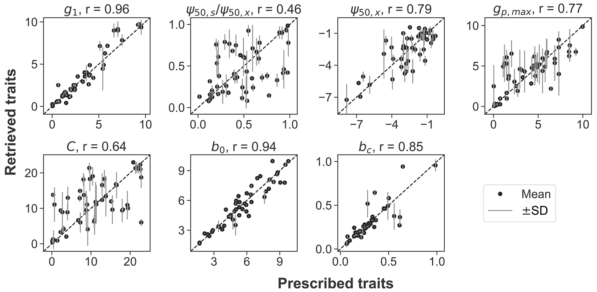
Figure 1 Comparison between the prescribed and retrieved plant hydraulic traits (g₁, ${\mathit{\psi }}_{\mathrm{50},\mathrm{s}}/{\mathit{\psi }}_{\mathrm{50},\mathrm{x}}$, ψ_50,x, g_p,max, and C) and soil properties (b₀ and b_c) in the observing system simulation experiment. The black dots and gray lines represent the mean and range of 1 standard deviation of the retrieved posterior distributions. The diagonal dashed line is the 1:1 line. Pearson correlation coefficient (r) between the prescribed and retrieved parameters is noted.

3.2 Accuracy of modeled VOD, ET, and surface soil moisture

Over the entire study period of 2003–2011, the coefficient of determination (R²) between estimated and observed VOD has a median of 0.38 and a mid-50 % range of (0.22,0.55) across the globe (Fig. 2a). The estimated VOD is highly correlated with observations in northern and southwestern Australia, northeastern China, India, central Europe, Africa, and eastern South America. The high VOD accuracy in these areas is likely partially a result of the large contribution of biomass to VOD due to strong biomass seasonality in these areas (Liu et al., 2011; Momen et al., 2017). Notably, however, even in areas where VOD has been shown to be less correlated with LAI, including central Australia, central Asia, southern Africa, and the western US (Momen et al., 2017), the estimated VOD accounting for the signature of leaf water potential is also able to capture observed VOD. The model also accurately estimates observed ET with a median R² of 0.60 and a mid-50 % range of (0.36,0.78; Fig. 2b). Unlike in the majority of the world, the R² of ET is relatively lower in central Australia, southern South America, and the southwestern US, where highly heterogeneous vegetation cover such as savannas and coexisting grass and shrubs within a pixel could undermine model accuracy. The median and mid-50 % range of surface soil moisture R² is 0.22 and (0.08,0.42), respectively. Modeled surface soil moisture is less accurate in croplands (likely due to irrigation) and in boreal regions, eastern China, Europe, and the mid-western and eastern US. These regions largely overlap with those where the observed soil moisture from AMSR-E is weakly correlated with the reanalysis product of ERA-Interim that integrates ground observations (Parinussa et al., 2015), suggesting greater uncertainties of surface soil moisture from AMSR-E compared to other regions. The overall accuracy of estimated VOD, ET, and surface soil moisture both within (Fig. S3) and outside (Fig. 2) the training period 2004–2005 suggest that the model and the derived traits effectively represent plant hydraulic dynamics.

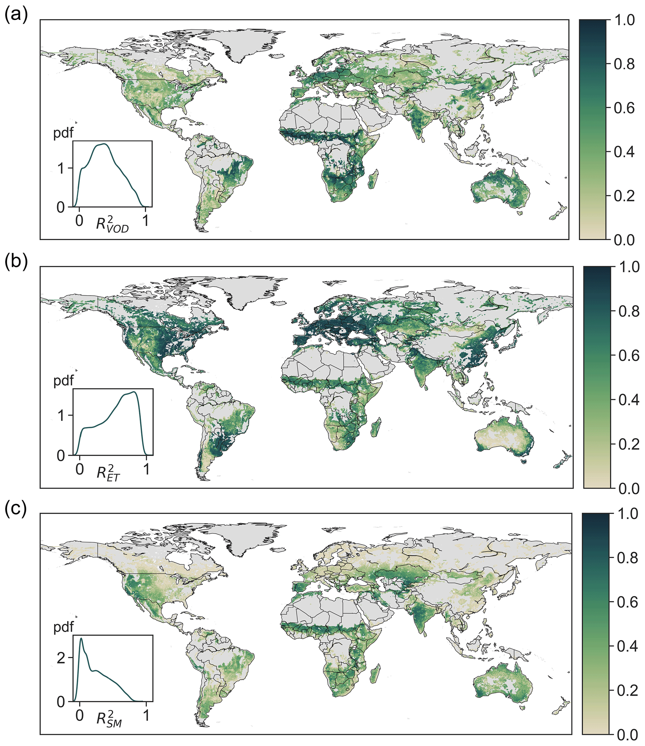
Figure 2 Assimilation accuracy (R²) of (a) VOD, (b) ET, and (c) soil moisture during the entire study period (2003–2011). Insets show the probability distribution (pdf) of R² across the entire study area. The gray shaded area is not included in analysis.

3.3 Global pattern of plant hydraulic traits

The retrieved stomatal conductance slope parameter g₁, which is inversely proportional to marginal water use efficiency (Eq. 6), exhibits clear spatial patterns (Fig. 3a). High g₁ values arise in areas covered by grasses and savannas, such as the western US, the Sahel, central Asia, northern Mongolia, and inner Australia. This pattern is consistent with predictions from experimental data and optimality theory that herbaceous species – given the low cost of stem wood construction per unit water transport – should have the largest g₁, i.e., be the least water-use efficient (Manzoni et al., 2011; Lin et al., 2015). In addition, croplands in India and eastern China also show high g₁, consistent with the high isohydricity of these regions (Konings and Gentine, 2017). Consistent with ground measurements that suggest g₁ increases with biome average temperature (Lin et al., 2015), the g₁ derived here is also (on average) lower in boreal ecosystems than in temperate and tropical ecosystems.

Highly negative ψ_50,x values are found in boreal evergreen needleleaf forests and in arid or seasonally dry biomes covered by forests, shrubs or savannas, such as the western US, central America, eastern south America, southeastern Africa, and Australia (Fig. 3b). However, ψ_50,x is more spatially scattered than g₁. This could partially arise from the greater coefficient of variation across ensembles of ψ_50,x (Fig. 4), suggesting ψ_50,x is less tightly constrained compared to g₁ (consistent with site-scale model–data fusion efforts in Liu et al. (2020a) and the uncertainty estimates in the OSSE; Fig. 1). This additional uncertainty might translate to more noise in the ensemble medians for ψ_50,x than that for g₁. Maps of other hydraulic traits are shown in Fig. S4. The patterns of hydraulic traits exhibit greater variability beyond PFT distribution (Fig. S2) and only limited correlation with soil and climate conditions (Fig. S5).

Among the plant hydraulic traits, we found strong coordination between the vulnerability of stomata and the xylem (ψ_50,s and ψ_50,x) across space (Fig. S5), consistent with existing evidence from ground measurements (Anderegg et al., 2017). Other hydraulic traits are only weakly correlated, including g_p,max and ψ_50,x (Fig. S5), which is consistent with the previous finding suggesting the safety–efficiency trade-off of xylem traits is weak across >400 species (Gleason et al., 2016).

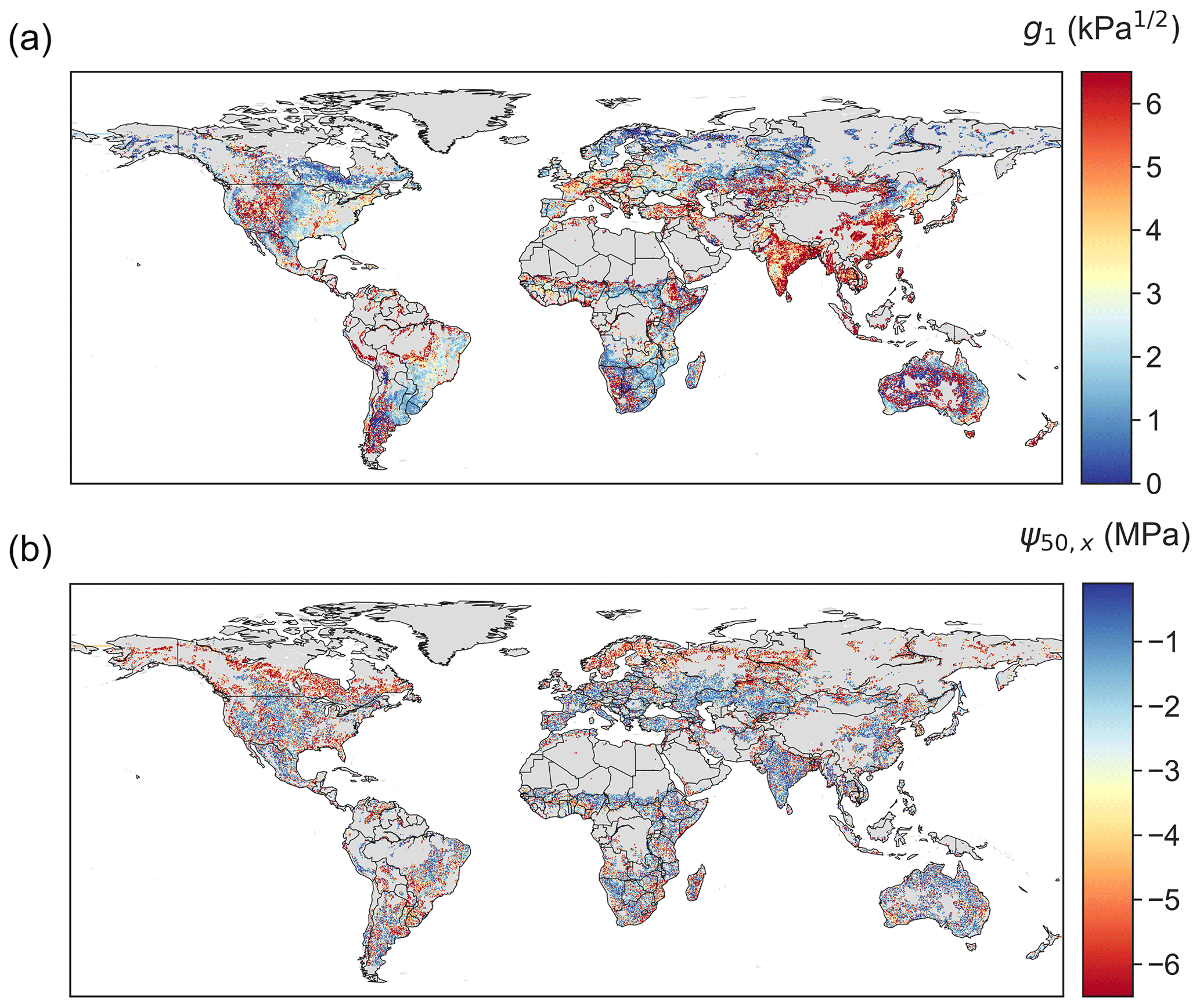
Figure 3 Global maps of (a) g₁ and (b) ψ_50,x retrieved using model–data fusion. The posterior mean of each pixel is plotted.

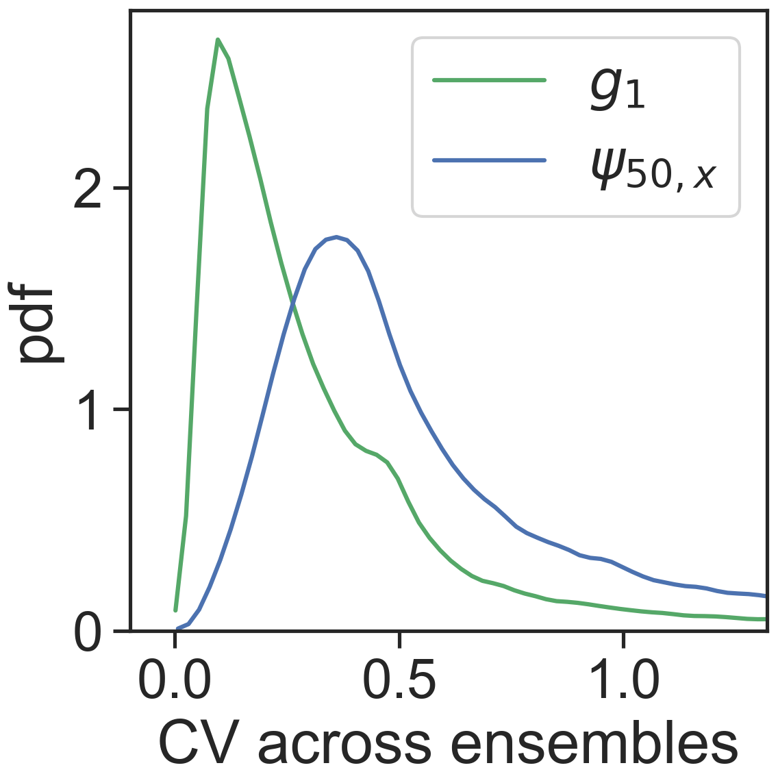
Figure 4 Empirical distribution across pixels of the coefficient of variation (CV) of g₁ and ψ_50,x calculated across ensembles.

Across PFTs, evergreen needleleaf forests have the lowest g₁, followed by deciduous broadleaf forests and shrublands (Fig. 5a). Grasslands and croplands have the highest g₁. This trend follows the across-PFT pattern found by Lin et al. (2015). The estimated across-PFT pattern of mean ψ_50,x is also consistent with measurements included in the TRY database (Kattge et al., 2011), i.e., lowest in grasslands and highest in evergreen needleleaf forests (Fig. 5b). However, across the globe, we found that the average standard deviation within PFTs is 3.6 and 2.3 times the standard deviation across PFTs for g₁ and ψ_50,x, respectively. The large within-PFT variation is consistent with in situ observations (Anderegg, 2015), indicating that PFTs are not informative of plant hydraulic traits.

We further compared the retrieved ψ_50,x for specific locations to an alternative estimate upscaled from Forest Inventory and Analysis (FIA) surveys (Fig. 6). Consistent with the FIA-based estimate, the retrieved ψ_50,x are overall lower in pixels dominated by evergreen needleleaf forests than in evergreen and deciduous broadleaf forests and mixed forests. However, across pixels, the ecosystem-scale ψ_50,x derived from remote sensing vary significantly more than the estimates from the Trugman et al. (2020) data set. Some fraction of this discrepancy might be due to intra-species variability in ψ_50,x, which is not accounted for in the FIA-based estimate, and due to the uncertainty in the kriging-based interpolation used for upscaling from the sparse FIA plots to each 1^∘ pixel. Nevertheless, this discrepancy highlights the scale gap between traits measured for a single plant and those derived for an ecosystem.

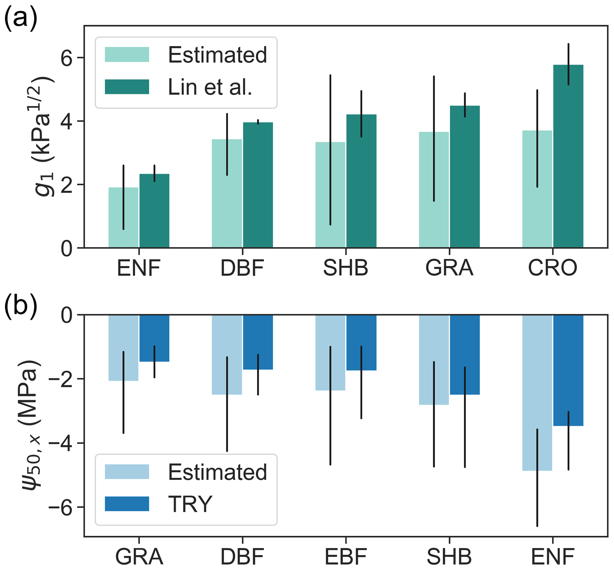
Figure 5 Retrieved (a) g₁ and (b) ψ_50,x using model–data fusion (light colored bars), grouped by PFTs, in comparison with values derived from in situ measurements (dark colored bars) reported in Lin et al. (2015) and the TRY database (Kattge et al., 2011). Compared PFTs include evergreen needleleaf forest (ENF), deciduous broadleaf forest (DBF), evergreen broadleaf forest (EBF), shrubland (SHB), grassland (GRA), and cropland (CRO). Bars represent medians of each PFT, and black lines indicate the 25th–75th percentile ranges. The g₁ averaged across gymnosperm trees and angiosperm trees from Lin et al. (2015) were compared to retrieved g₁ in pixels dominated by ENF and DBF, respectively.

Figure 6 Aggregated ψ_50,x from upscaling the Forest Inventory and Analysis (FIA) plots, based on Trugman et al. (2020), and ψ_50,x retrieved here for corresponding pixels. The point size is scaled by number of plots used in aggregation for each pixel.

3.4 Hydraulic functional types (HFTs)

We built six HFTs (termed H1 to H6) using the K-means clustering method. The number of clusters (six) was chosen, using the elbow method, based on the inflection point of the ratio of within- to across-cluster variance (Fig. S6). Across the six HFTs, the across-cluster variance is 1.7 times as large as the within-cluster variance. The HFTs explain 57 % of the total variance in hydraulic traits across the globe. The cluster centers of the six HFTs are characterized by distinct combinations of hydraulic traits (Fig. 7a). Specifically, H1 and H2 feature low ψ_50,s and ψ_50,x and are mainly distributed in boreal forest and arid or seasonally dry biomes, including the western US, central America, southeastern Africa, central Asia, and Australia (Fig. 7b). H3 and H4 are characterized by low and high vegetation capacitance (C), respectively, though both have low g_p,max. H3 is mainly but not exclusively distributed in grasslands and savannas in the central US, the Nordeste region in Brazil, eastern and southern Africa, and eastern Australia, as well as in the Miombo woodlands. H4 is distributed in shrublands in the southwestern US, Argentina, southern Africa, northwestern India, and northeastern Australia. H5, often found in tropical and subtropical regions, is characterized by large g_p,max and capacitance. H6 is characterized primarily by high g₁, which includes croplands in India, southeastern Asia, and central and eastern China. Note that the pattern of HFTs (Fig. 7b) is substantially distinct from the distribution of PFTs (Fig. S2), illustrating the limitations of parameterizing plant hydraulics based on PFTs.

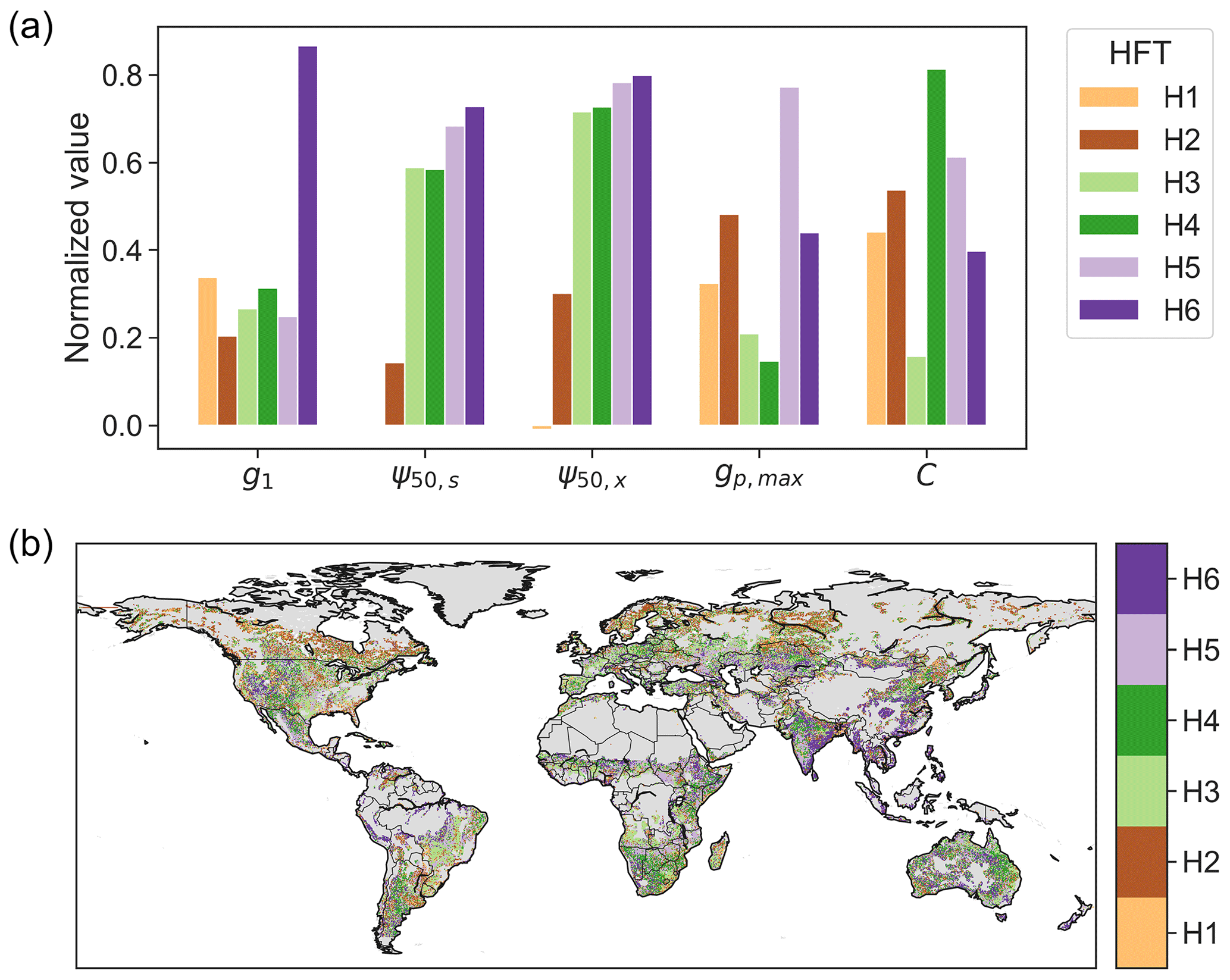
Figure 7 (a) Plant hydraulic traits of the centers of six hydraulic functional types and (b) their spatial pattern. Each trait of cluster centers is normalized using $(V-V_{\mathrm{5}})/(V_{\mathrm{95}}-V_{\mathrm{5}})$, where V is the trait magnitude, and V₅ and V₉₅ are the 5th and 95th percentiles of the corresponding trait across the study area.

Using averaged traits per PFT, instead of pixel-specific traits to calculate VOD and ET, led to a median increase in normalized root mean square error (nRMSE, with the long-term average used for normalization) of 0.82 and 0.58, respectively. This degradation of accuracy is unsurprising given the high spatial variability in hydraulic traits and the fact that PFTs are not categorized specifically to distinguish plant hydraulic functions. However, using the hydraulic traits averaged per HFT instead improves prediction accuracy over the PFT-based predictions. When compared to using pixel-specific values, using average traits based on HFTs increases the nRMSE by 0.65 and 0.42 for VOD and ET, respectively. In each case, this is less than the degradation when PFT-based averages are used. Indeed, when PFT-based instead of HFT-based model estimates are compared, the nRMSE of ET increases by more than 0.1 in 58 % of the analyzed area (Fig. 8a). ET is mainly improved in arid or seasonally dry biomes, including the western US, southern South America, southern and eastern Africa, central Asia, and Australia. In addition, the nRMSE of VOD is also improved by more than 0.5 in 37 % of the analyzed area using HFTs rather than PFTs (Fig. 8b). Areas exhibiting reduced error are mainly located in the southwestern US, central America, eastern South America, the Mediterranean, Africa, and Australia, where variation in leaf water potential has a strong signature on VOD (Momen et al., 2017). These findings suggest the importance of the appropriate parameterization of hydraulic traits on capturing leaf water potential and ET variations at an ecosystem scale.

Figure 8 Normalized root mean square error (nRMSE) of estimated (a) ET and (b) VOD, using traits averaged by plant PFTs minus those using traits averaged by HFTs. The insets show the areal frequency of the nRMSE difference.

4 Discussion

4.1 Contribution of VOD to informing plant hydraulic behavior

The fact that VOD varies with plant water content allows the investigation of plant physiological dynamics at large scales. Although VOD has often been used as a proxy of aboveground biomass (e.g., Liu et al., 2015; Tian et al., 2017; Brandt et al., 2018; Teubner et al., 2019), it is in fact determined by both biomass and plant water status (Konings et al., 2019). VOD variations within a day (Konings and Gentine, 2017; Li et al., 2017; Anderegg et al., 2018) and during soil drydowns (Feldman et al., 2018; Zhang et al., 2019; Feldman et al., 2020) highlight the sensitivity of VOD to relative water content. At seasonal and interannual scales, VOD has also been found to be modulated by leaf water potential or relative water content, thus deviating from biomass signals (Momen et al., 2017; Tian et al., 2018; Tong et al., 2019). Here, after parsing out the impact of biomass through LAI, VOD provides information about leaf water potential variation and, therefore, contributes to constraining the underlying hydraulic traits. Kumar et al. (2020) previously assimilated VOD into a land surface model as a constraint on biomass, which led to improvements in modeled ET. Our findings suggest that, when assimilated into models with an explicit representation of plant hydraulics, VOD can act to constrain both water and carbon dynamics and their respective climatic responses. Although not explored in detail in this study, note also that, by determining optimal values for a, b, and c (the parameters relating VOD to ψ_l in Eq. 11), the model–data fusion system introduced here also allows the determination of ψ_l from VOD, which may be of interest for a variety of studies of plant responses to drought. However, additional research is needed to understand the effect of the choice of retrieval algorithm and specific VOD product (Li et al., 2021) on any inferred VOD–ψ_l relationships. For this reason, any such efforts would also benefit from explicit uncertainty quantification.

Our previous study (Liu et al., 2020a) at the stand scale has shown that stomatal traits are well constrained using ET alone, whereas xylem traits, including ψ_50,x, remain largely under-constrained, in part due to lack of information on leaf water potential. Incorporating VOD among the constraints here contributes to the separation of xylem and stomatal behavior. As a result, the model–data fusion approach here is, to our knowledge, the first to be able to retrieve both stomatal and xylem traits across the globe. Nevertheless, ψ_50,x is still less well resolved across ensembles compared to other traits (Fig. 4). This could result from trade-offs among hydraulic traits and the lack of constraints on the scaling from leaf water potential to VOD, which varies across space. More prior information about these two factors will likely contribute to improved retrieval of plant hydraulic traits. Additionally, the use of solar-induced fluorescence or other constraints on photosynthesis may allow for independent information about stomatal closure that could be used to improve the accuracy and certainty of the retrieved hydraulic traits. However, care should be taken that the uncertainty introduced by coupling to a photosynthesis model does not outweigh the added advantage of this additional constraint.

4.2 Bridging the spatial scale gap of hydraulic traits

Plant hydraulic traits vary among segments from root to shoot even for a single tree, causing the hydraulic sensitivity at a whole-tree scale to be distinct from that measured at a segment scale (Johnson et al., 2016). Similarly, species diversity, canopy structure, and demographic composition can cause large variability in hydraulic traits. As a result, a community-weighted average of a trait may not well represent the integrated hydraulic behavior at an ecosystem scale, as evidenced, for example, by the significant effect of plant hydraulic diversity on evapotranspiration responses to drought (Anderegg et al., 2018). Here, we also found a substantial discrepancy between community-weighted ψ_50,x and the ecosystem-scaled value derived from representing the property of the entire pixel, even in the most extensively surveyed pixels available (biggest dots in Fig. 6). This highlights the challenge of scaling up ground measurements of plant hydraulic traits to a scale relevant to land surface modeling from the bottom up. The model–data fusion used here provides an approach to help address this challenge. However, further study is needed to explore how stand and ecosystem characteristics shape the ecosystem-scale hydraulic traits, as well as the effective relationship between leaf water potential and remote-sensing-scale water content.

4.3 Implications for land surface models

Because they are able to predict ET and VOD better than PFTs (Fig. 8), the HFTs point to the potential for a better parameterization scheme of plant hydraulics in land surface models. Because HFTs require fewer clusters than PFTs do to model ET with the same or better accuracy, parameterizing plant hydraulics by HFTs in land surface models may contribute to higher model accuracy. However, because the magnitude of state variables may differ between models, even as their temporal dynamics do not (Koster et al., 2009), including between a given land surface model and the model used here, using the exact values derived here may cause errors. Instead, the map of HFTs and their relative magnitude of traits can be used as a baseline for model-specific calibration. Moreover, moving beyond fixed values for each HFT, hydraulic traits within each type may be further related to landscape features such as climate, topography, canopy height, and stand age using the environmental filtering approach (Butler et al., 2017). As demonstrated for photosynthetic traits (Verheijen et al., 2013; Smith et al., 2019), such relationships allow practical flexibility to account for trait variations across space, thus improving the performance of large-scale models. They may also allow improved compatibility with subgrid tiling schemes used by land surface schemes. As land surface models that explicitly represent plant hydraulics are becoming more common, our results demonstrate the possibility of alternative, computationally efficient approaches to parameterizing plant hydraulic behavior, which will contribute to improved prediction of natural resources and climate feedbacks.

5 Conclusions

This study derived ecosystem-scale plant hydraulic traits across the globe using a model–data fusion approach. The retrieved traits enable our hydraulic model to capture the dynamics of leaf water potential and ET, based on a comparison to remote sensing observations. While the traits derived here are consistent with across-PFT patterns based on in situ measurements, they also exhibit large within-PFT variations (as expected). There is some discrepancy between our derived ψ_50,x and the values derived from interpolating between forest inventory plots, though it is unclear if this discrepancy is caused by errors in the model–data fusion retrievals, errors in the upscaled inventory data due to intra-specific variability and spatial interpolation imperfections, or both. Uncertainty is also induced by whether or not our retrievals represent the same effective values as a community-weighted average (see Sect. 4.2). Nevertheless, reasonable correspondence between the across-PFT variations in our derived traits compared to in situ measurements add confidence to the data set introduced here.

As an alternative to PFTs, we constructed hydraulic functional types based on clustering of the derived hydraulic traits. Using the hydraulic functional types, rather than PFTs, to drive averaged traits by functional types improves the accuracy of estimated ET and VOD, even as the number of functional types is reduced relative to a PFT-based representation. This suggests that hydraulic functional types may form a computationally efficient yet promising approach for representing the diversity of plant hydraulic behavior in large-scale land surface models. We note that the exact values of the derived hydraulic traits depend on the specific data and model representation used here and, therefore, are subject to model and data uncertainties. However, our findings highlight opportunities and challenges for further investigation of plant hydraulics at a global scale.