the Creative Commons Attribution 4.0 License.
the Creative Commons Attribution 4.0 License.
 | 19 Apr 2021
Rainfall–runoff prediction at multiple timescales with a single Long Short-Term Memory network
Frederik Kratzert
Daniel Klotz
Grey Nearing
Jimmy Lin
Sepp Hochreiter
Long Short-Term Memory (LSTM) networks have been applied to daily discharge prediction with remarkable success. Many practical applications, however, require predictions at more granular timescales. For instance, accurate prediction of short but extreme flood peaks can make a lifesaving difference, yet such peaks may escape the coarse temporal resolution of daily predictions. Naively training an LSTM on hourly data, however, entails very long input sequences that make learning difficult and computationally expensive. In this study, we propose two multi-timescale LSTM (MTS-LSTM) architectures that jointly predict multiple timescales within one model, as they process long-past inputs at a different temporal resolution than more recent inputs. In a benchmark on 516 basins across the continental United States, these models achieved significantly higher Nash–Sutcliffe efficiency (NSE) values than the US National Water Model. Compared to naive prediction with distinct LSTMs per timescale, the multi-timescale architectures are computationally more efficient with no loss in accuracy. Beyond prediction quality, the multi-timescale LSTM can process different input variables at different timescales, which is especially relevant to operational applications where the lead time of meteorological forcings depends on their temporal resolution.
- Article
(1820 KB) - Full-text XML
- BibTeX
- EndNote


Rainfall–runoff modeling approaches based on deep learning – particularly Long Short-Term Memory (LSTM) networks – have proven highly successful in a number of studies. LSTMs can predict hydrologic processes in multiple catchments using a single model and yield more accurate predictions than state-of-the-art process-based models in a variety of benchmarks (Kratzert et al., 2019).
Different applications require hydrologic information at different timescales. For example, hydropower operators might care about daily or weekly (or longer) inputs into their reservoirs, while flood forecasting requires sub-daily predictions. Yet, much of the work in applying deep learning to streamflow prediction has been at the daily timescale. Daily forecasts make sense for medium- to long-range forecasts; however, daily input resolution mutes diurnal variations that may cause important variations in discharge signatures, such as evapotranspiration and snowmelt. Thus, daily predictions are often too coarse to provide actionable information for short-range forecasts. For example, in the event of flooding, the distinction between moderate discharge spread across the day and the same amount of water compressed into a few hours of flash flooding may pose a life-threatening difference.
Because of this, hydrologic models often operate at multiple timescales using several independent setups of a traditional, process-based rainfall–runoff model. For instance, the US National Oceanic and Atmospheric Administration’s (NOAA) National Water Model (NWM) produces hourly short-range forecasts every hour, as well as three- and six-hourly medium- to long-range forecasts every 6 h (Cosgrove and Klemmer, 2019; Salas et al., 2018). A similar approach could be used for machine learning models, but this has several disadvantages. Namely, this would require a distinct deep learning model per timescale, which means that computational resource demands multiply with the number of predicted timescales. Further, since the models cannot exchange information, predictions have the potential to be inconsistent across timescales.
Another challenge in operational scenarios stems from the fact that in many cases multiple sets of forcing data are available. Ideally, a model should be able to process all forcings products together, such that it can combine and correlate information across products and obtain better estimates of the true meteorologic conditions (e.g., Kratzert et al., 2020). Since different meteorological data products are often available at different timescales, models should not only be able to produce predictions at multiple timescales, but also to process inputs at different temporal resolutions.
The issue of multiple input and output timescales is well-known in the field of machine learning (we refer readers with a machine learning or data science background to Gauch and Lin (2020) for a general introduction to rainfall–runoff modeling). The architectural flexibility of recurrent neural models allows for approaches that jointly process the different timescales in a hierarchical fashion. Techniques to “divide and conquer” long sequences through hierarchical processing date back decades (e.g., Schmidhuber, 1991; Mozer, 1991). More recently, Koutník et al. (2014) proposed an architecture that efficiently learns long- and short-term relationships in time series. Those authors partitioned the internals of their neural network into different groups, where each group was updated on individual, pre-defined, intervals. However, the whole sequence was still processed on the highest frequency, which makes training slow. Chung et al. (2016) extended the idea of hierarchical processing of multiple timescales: in their setup, the model adjusts its updating rates to the current input, e.g., to align with words or handwriting strokes. A major limitation of this approach is that it requires a binary decision about whether to make an update or not, which complicates the training procedure. Neil et al. (2016) proposed an LSTM architecture with a gating mechanism that allows state and output updates only during time slots of learned frequencies. For time steps where the gate is closed, the old state and output are reused. This helps discriminate superimposed input signals, but is likely unsuited for rainfall–runoff prediction because no aggregation takes place while the time gate is closed. In a different research thread, Graves et al. (2007) proposed a multidimensional variant of LSTMs for problems with more than one temporal or spatial dimension. Framed in the context of multi-timescale prediction, one could define each timescale as one temporal dimension and process the inputs at all timescales simultaneously. Like the hierarchical approaches, however, this paradigm would process the full time series at all timescales and thus lead to slow training.
Most of the models discussed above were designed for tasks like natural language processing and other non-physical applications. Unlike these tasks, time series in rainfall–runoff modeling have regular frequencies with fixed translation factors (e.g., one day always has 24 h), whereas words in natural language or strokes in handwriting vary in their length. The application discussed by Araya et al. (2019) was closer in this respect – they predicted hourly wind speeds given input data at multiple timescales. However, like the aforementioned language and handwriting applications, the objective in this case was to predict a single time series – be it sentences, handwriting strokes, or wind speed. Our objective encompasses multiple outputs, one for each target timescale. In this regard, multi-timescale rainfall–runoff prediction has similarities to multi-objective optimization. The different objectives (predictions at different frequencies) are closely related, since aggregation of discharge across time steps should be conservative: for instance, every group of 24 hourly prediction steps should average (or sum, depending on the units) to one daily prediction step. Rather than viewing the problem from a multi-objective perspective, Lechner and Hasani (2020) modeled time-continuous functions with ODE-LSTMs, a method that combines LSTMs with a mixture of ordinary differential equations and recurrent neural networks (ODE-RNN). The resulting models generate continuous predictions at arbitrary granularity. Initially, this seems like a highly promising approach; however, it has several drawbacks in our application. First, since one model generates predictions for all timescales, it is not straightforward to use different forcings products for different timescales. Second, ODE-LSTMs were originally intended for scenarios where the input data arrives at irregular intervals. In our context, the opposite is true: meteorological forcing data generally have fixed, regular frequencies. Also, for practical purposes we do not actually need predictions at arbitrary granularity – a fixed set of target timescales is generally sufficient for hydrologic applications. Lastly, in our exploratory experiments (see Appendix C), using ODE-LSTMs to predict at timescales that were not part of training was actually worse (and much slower) than (dis-)aggregating the fixed-timescale predictions of our proposed models (we report our exploration of ODE-LSTMs in Appendix C).
In this paper, we show how LSTM-based architectures can jointly predict discharge at multiple timescales in one model while leveraging meteorological inputs at different timescales. We make the following contributions:
-
First, we outline two LSTM architectures that predict discharge at multiple timescales (Sect. 2.3). We capitalize on the fact that watersheds are damped systems: while the history of total mass and energy inputs are important, the impact of high-frequency variation becomes less important the farther we look back. Our approach to providing multiple output timescales processes long-past input data at coarser temporal resolution than recent time steps. This shortens the input sequences, since high-resolution inputs are only necessary for the last few time steps. We benchmark daily and hourly predictions from these models against (i) a naive deep learning solution that trains individual LSTMs for each timescale and (ii) a traditional hydrologic model, the US National Water Model (Sect. 3.1).
-
Second, we propose a regularization scheme that reduces inconsistencies across timescales as they arise from naive, per-timescale prediction (Sect. 2.3.2).
-
Third, we demonstrate that our multi-timescale LSTMs can ingest individual and multiple sets of forcing data for each target timescale, where each forcing product has regular but possibly individual time intervals. This closely resembles operational forecasting use cases where forcings with high temporal resolution often have shorter lead times than forcings with low resolution (Sect. 3.4).
2.1 Data
To maintain some degree of continuity and comparability with previous benchmarking studies (Newman et al., 2017; Kratzert et al., 2019), we conducted our experiments on the CAMELS dataset (Newman et al., 2014a; Addor et al., 2017a) in a way that is as comparable as possible. The CAMELS dataset, however, provides discharge data only at daily timescales. Out of the 531 CAMELS benchmarking basins used by previous studies, 516 basins have hourly stream gauge data available from the USGS Water Information System through the Instantaneous Values REST API (United States Geological Survey, 2021). This USGS service provides historical measurements at varying sub-daily resolutions (usually every 15 to 60 min), which we averaged to hourly and daily time steps for each basin. Since our forcing data and benchmark model data use UTC timestamps, we converted the USGS streamflow timestamps to UTC. All discharge information used in this study was downloaded from the USGS API. We did not use the discharge from the CAMELS dataset, however, we chose only basins that are included in the CAMELS dataset.
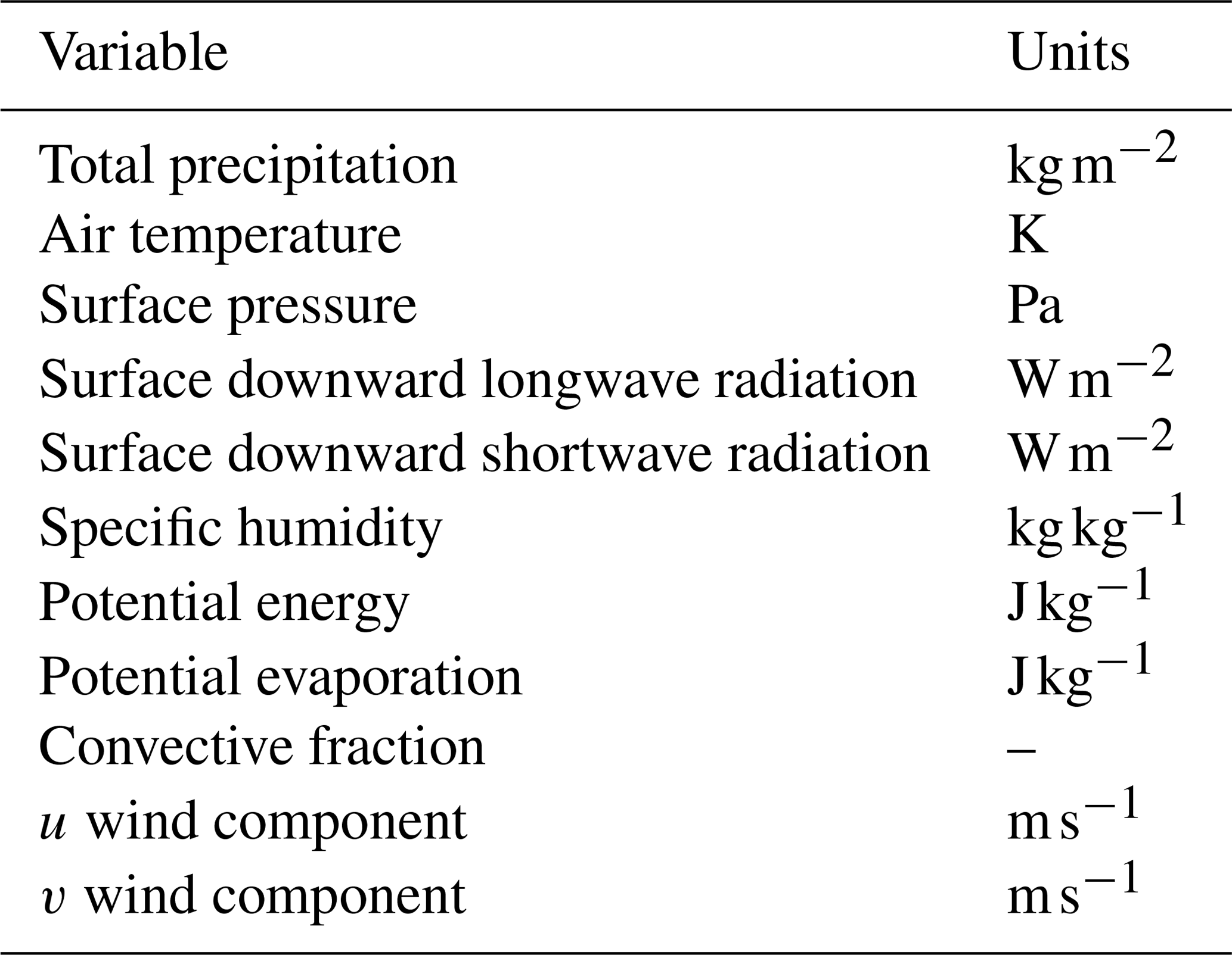
While CAMELS provides only daily meteorological forcing data, we needed hourly forcings. To maintain some congruence with previous CAMELS experiments, we used the hourly NLDAS-2 product, which contains hourly meteorological data since 1979 (Xia et al., 2012). We spatially averaged the forcing variables listed in Table 1 for each basin. Additionally, we averaged these basin-specific hourly meteorological variables to daily values.
Table 1NLDAS forcing variables used in this study (Xia et al., 2012).
Following common practice in machine learning, we split the dataset into training, validation, and test periods. We used the training period (1 October 1990 to 30 September 2003) to fit the models given a set of hyperparameters. Then, we applied the models to the validation period (1 October 2003 to 30 September 2008) to evaluate their accuracy on previously unseen data. To find the ideal hyperparameters, we repeated this process several times (with different hyperparameters; see Appendix D) and selected the model that achieved the best validation accuracy. Only after hyperparameters were selected for a final model on the validation dataset did we apply any trained model(s) to the test period (1 October 2008 to 30 September 2018). This way, the model had never seen the test data during any part of the development or training process, which helps avoid overfitting.
All LSTM models used in this study take as inputs the 11 forcing variables listed in Table 1, concatenated at each time step with the same 27 static catchment attributes from the CAMELS dataset that were used by Kratzert et al. (2019).
2.2 Benchmark models
We used two groups of models as baselines for comparison with the proposed architectures: the LSTM proposed by Kratzert et al. (2019), naively adapted to hourly streamflow modeling, and the NWM, a traditional hydrologic model used operationally by the National Oceanic and Atmospheric Administration (Cosgrove and Klemmer, 2019).
2.2.1 Traditional hydrologic model
The US National Oceanic and Atmospheric Agency (NOAA) generates hourly streamflow predictions with the NWM (Salas et al., 2018), which is a process-based model based on WRF-Hydro (Gochis et al., 2020). Specifically, we benchmarked against the NWM v2 reanalysis product, which includes hourly streamflow predictions for the years 1993 through 2018. For these predictions, the NWM was calibrated on meteorological NLDAS forcings for around 1500 basins and then regionalized to around 2.7 million outflow points (source: personal communication with scientists from NOAA, 2021). To obtain predictions at lower (e.g., daily) temporal resolutions, we averaged the hourly predictions.
2.2.2 Naive LSTM
Long Short-Term Memory (LSTM) networks (Hochreiter and Schmidhuber, 1997) are a flavor of recurrent neural networks designed to model long-term dependencies between input and output data. LSTMs maintain an internal memory state that is updated at each time step by a set of activated functions called gates. These gates control the input–state relationship (through the input gate), the state–output relationship (through the output gate), and the memory timescales (through the forget gate). Figure 1 illustrates this architecture. For a more detailed description of LSTMs, especially in the context of rainfall–runoff modeling, we refer to Kratzert et al. (2018).
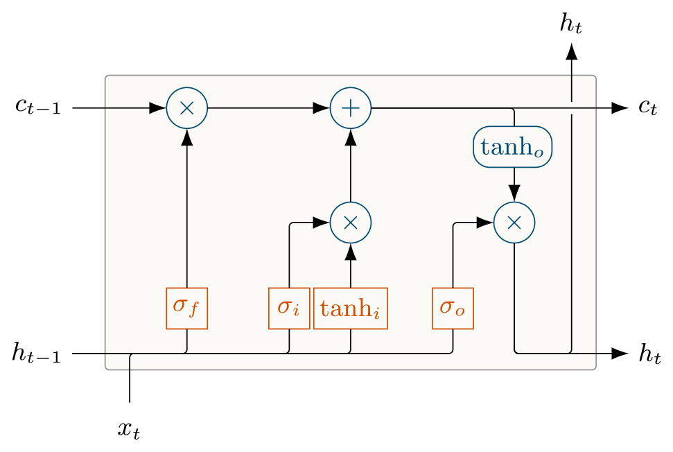
LSTMs can cope with longer time series than classic recurrent neural networks because they are not susceptible to vanishing gradients during the training procedure (Bengio et al., 1994; Hochreiter and Schmidhuber, 1997). Since LSTMs process input sequences sequentially, longer time series result in longer training and inference time. For daily predictions, this is not a problem, since look-back windows of 365 d appear to be sufficient for most basins, at least in the CAMELS dataset. Therefore, our baseline for daily predictions is the LSTM model from Kratzert et al. (2020), which was trained on daily data with a look-back of 365 d.
For hourly data, even half a year corresponds to more than 4300 time steps, which results in very long training and inference runtime, as we will detail in Sect. 3.3. In addition to the computational overhead, the LSTM forget gate makes it hard to learn long-term dependencies, because it effectively reintroduces vanishing gradients into the LSTM (Jozefowicz et al., 2015). Yet, we cannot simply remove the forget gate – both empirical LSTM analyses (Jozefowicz et al., 2015; Greff et al., 2017) and our exploratory experiments (unpublished) showed that this deteriorates results. To address this, Gers et al. (1999) proposed to initialize the bias of the forget gate to a small positive value (we used 3). This starts training with an open gate and enables gradient flow across more time steps.
We used this bias initialization trick for all our LSTM models, and it allowed us to include the LSTM with hourly inputs as the naive hourly baseline for our proposed models. The architecture for this naive benchmark is identical to the daily LSTM, except that we ingested input sequences of 4320 h (180 d). Further, we tuned the learning rate and batch size for the naive hourly LSTM, since it receives 24 times the amount of samples than the daily LSTM. The extremely slow training impedes a more extensive hyperparameter search. Appendix D details the grid of hyperparameters we evaluated to find a suitable configuration, as well as further details on the final hyperparameters.
2.3 Using LSTMs to predict multiple timescales
We evaluated two different LSTM architectures that are capable of simultaneous predictions at multiple timescales. For the sake of simplicity, the following explanations use the example of a two-timescale model that generates daily and hourly predictions. Nevertheless, the architectures we describe here generalize to other timescales and to more than two timescales, as we will show in an experiment in Sect. 3.5.
The first model, shared multi-timescale LSTM (sMTS-LSTM), is a simple extension of the naive approach. Intuitively, it seems reasonable that the relationships that govern daily predictions hold, to some extent, for hourly predictions as well. Hence, it may be possible to learn these dynamics in a single LSTM that processes the time series twice: once at a daily resolution and again at an hourly resolution. Since we model a system where the resolution of long-past time steps is less important, we can simplify the second (hourly) pass by reusing the first part of the daily time series. This way, we only need to use hourly inputs for the more recent time steps, which yields shorter time series that are easier to process. From a more technical point of view, we first generate a daily prediction as usual – the LSTM ingests an input sequence of TD time steps at daily resolution and outputs a prediction at the last time step (i.e., sequence-to-one prediction). Next, we reset the hidden and cell states to their values from time step and ingest the hourly input sequence of length TH to generate 24 predictions on an hourly timescale that correspond to the last daily prediction. In other words, we reuse the initial daily time steps and use hourly inputs only for the remaining time steps. To summarize this approach, we perform two forward passes through the same LSTM at each prediction step: one that generates a daily prediction and one that generates 24 corresponding hourly predictions. Since the same LSTM processes input data at multiple timescales, the model needs a way to identify the current input timescale and distinguish daily from hourly inputs. For this, we add a one-hot timescale encoding to the input sequence. The key insight with this model is that the hourly forward pass starts with LSTM states from the daily forward pass, which act as a summary of long-term information up to that point. In effect, the LSTM has access to a large look-back window but, unlike the naive hourly LSTM, it does not suffer from the performance impact of extremely long input sequences.
The second architecture, illustrated in Fig. 2, is a more general variant of the sMTS-LSTM that is specifically built for multi-timescale predictions. We call this a multi-timescale LSTM (MTS-LSTM). The MTS-LSTM architecture stems from the idea that the daily and hourly predictions may behave differently enough that it may be challenging for one LSTM to learn dynamics at both timescales, as is required for the sMTS-LSTM. Instead, we hypothesize that it may be easier to process inputs at different timescales using an individual LSTM per timescale. The MTS-LSTM does not perform two forward passes (as sMTS-LSTM does). Instead, it uses the cell states and hidden states of a daily LSTM to initialize an hourly LSTM after some number of initial daily time steps (see Fig. 2). More technically, we first generate a prediction with an LSTM acting at the coarsest timescale (here, daily) using a full input sequence of length TD (e.g., 365 d). Next, we reuse the daily hidden and cell states from time step as the initial states for an LSTM at a finer timescale (here, hourly), which generates the corresponding 24 hourly predictions. Since the two LSTM branches may have different hidden sizes, we feed the states through a linear state transfer layer (FCh, FCc) before reusing them as initial hourly states. In this setup, each LSTM branch only receives inputs of its respective timescale (i.e., separate weights and biases are learned for each input timescale), hence, we do not need to use a one-hot encoding to represent the timescale.
Effectively, the sMTS-LSTM is an ablation of the MTS-LSTM. The sMTS-LSTM is an MTS-LSTM where the different LSTM branches all share the same set of weights and states are transferred without any additional computation (i.e., the transfer layers FCh and FCc are identity functions). Conversely, the MTS-LSTM is a generalization of sMTS-LSTM. Consider an MTS-LSTM that uses the same hidden size in all branches. In theory, this model could learn to use identity matrices as transfer layers and to use equal weights in all LSTM branches. Except for the one-hot encoding, this would make it an sMTS-LSTM.
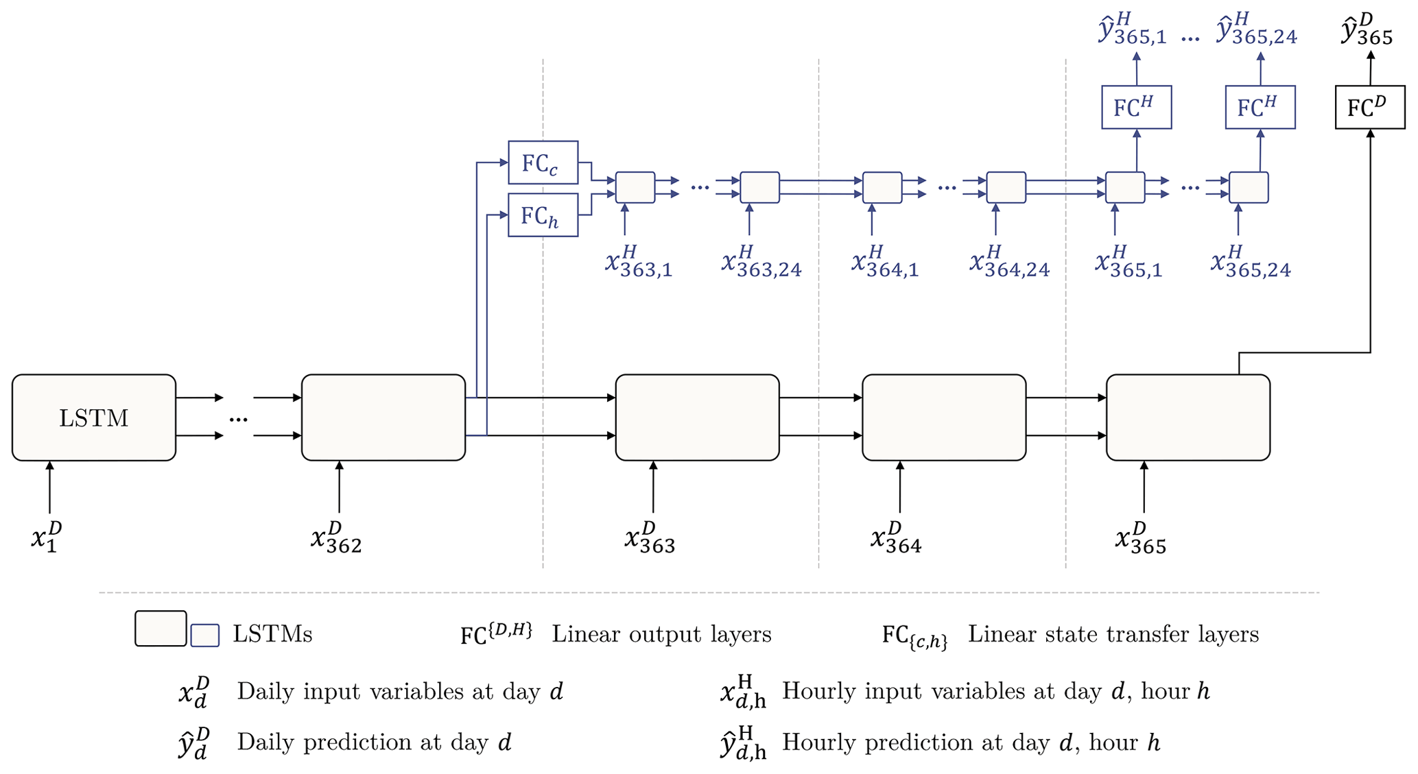
Figure 2Illustration of the MTS-LSTM architecture that uses one distinct LSTM per timescale. In the depicted example, the daily and hourly input sequence lengths are TD=365 and TH=72 (we chose this value for the sake of a tidy illustration; the benchmarked model uses TH=336). In the sMTS-LSTM model (i.e., without distinct LSTM branches), FCc and FCh are identity functions, and the two branches (including the fully connected output layers FCH and FCD) share their model weights.
2.3.1 Per-timescale input variables
An important advantage of the MTS-LSTM over the sMTS-LSTM architecture arises from its more flexible input dimensionality. Since sMTS-LSTM processes each timescale with the same LSTM, the inputs at all timescales must have the same number of variables. MTS-LSTM, on the other hand, processes each timescale in an individual LSTM branch and can therefore ingest different input variables to predict the different timescales. This can be a key differentiator in operational applications when, for instance, there exist daily weather forecasts with a much longer lead time than the available hourly forecasts, or when using remote sensing data that are available only at certain overpass frequencies. Input products available at different time frequencies will generally have different numbers of variables, so sMTS-LSTM could only use the products that are available for the highest resolution (we can usually obtain all other resolutions by aggregation). In contrast, MTS-LSTM can process daily forcings in its daily LSTM branch and hourly forcings in its hourly LSTM branch – regardless of the number of variables – since each branch can have a different input size. As such, this per-timescale forcings strategy allows for using different inputs at different timescales.
To evaluate this capability, we used two sets of forcings as daily inputs: the Daymet and Maurer forcing sets that are included in the CAMELS dataset (Newman et al., 2014a). For lack of other hourly forcing products, we conducted two experiments: in one, we continued to use only the hourly NLDAS forcings. In the other, we ingested the same hourly NLDAS forcings as well as the corresponding day’s Daymet and Maurer forcings at each hour (we concatenated the daily values to the inputs at each hour of the day). Since the Maurer forcings only range until 2008, we conducted this experiment on the validation period from October 2003 to September 2008.
2.3.2 Cross-timescale consistency
Since the MTS-LSTM and sMTS-LSTM architectures generate predictions at multiple timescales simultaneously, we can incentivize predictions that are consistent across timescales using loss regularization. Unlike in other domains (e.g., computer vision; Zamir et al., 2020), consistency is well-defined in our application: predictions are consistent if the mean of every day’s hourly predictions is the same as that day’s daily prediction. Hence, we can explicitly state this constraint as a regularization term in our loss function. Building on the basin-averaged NSE loss from Kratzert et al. (2019), our loss function averages the losses from each individual timescale and regularizes with the mean squared difference between daily and day-averaged hourly predictions. Note that although we describe the regularization with only two simultaneously predicted timescales, the approach generalizes to more timescales, as we can add the mean squared difference between each pair of timescale τ and next-finer timescale τ′. All taken together, we used the following loss for a two-timescale daily–hourly model:
Here, B is the number of basins, is the number of samples for basin b at timescale τ, and and are observed and predicted discharge values for the tth time step of basin b at timescale τ. σb is the observed discharge variance of basin b over the whole training period and ϵ is a small value that guarantees numeric stability. We predicted discharge in the same unit (mm h−1) at all timescales, so that the daily prediction is compared with an average across 24 h.
2.3.3 Predicting more timescales
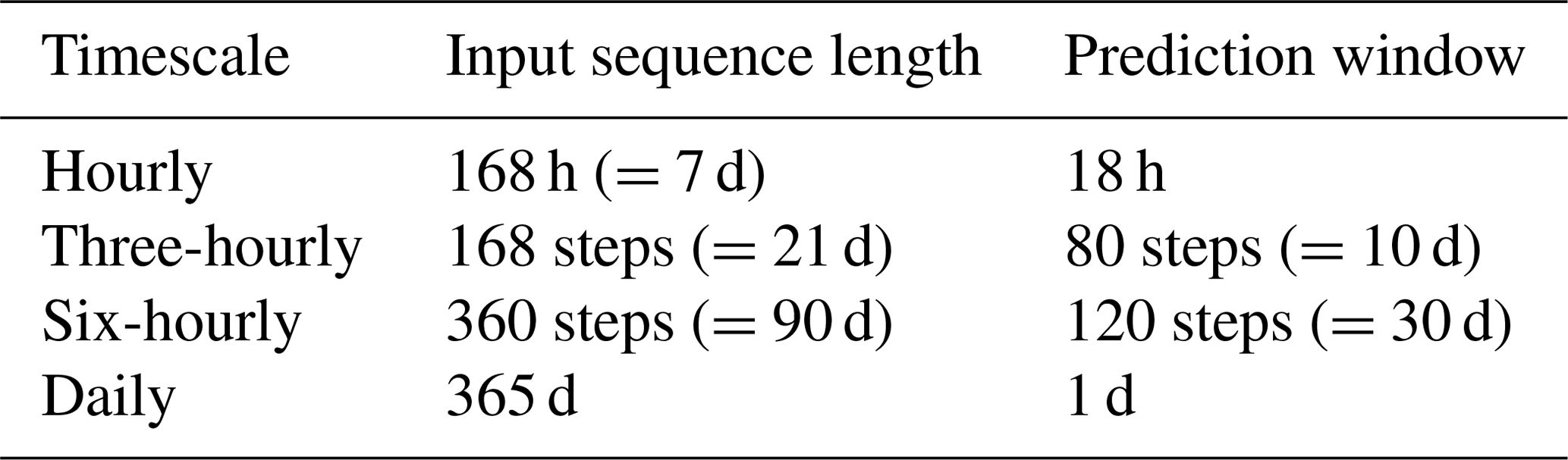
While all our experiments so far considered daily and hourly input and output data, the MTS-LSTM architecture generalizes to other timescales. To demonstrate this, we used a setup similar to the operational NWM, albeit in a reanalysis setting: we trained an MTS-LSTM to predict the last 18 h (hourly), 10 d (three-hourly), and 30 d (six-hourly) of discharge – all within one MTS-LSTM. Table 2 details the sizes of the input and output sequences for each timescale. To achieve a sufficiently long look-back window without using exceedingly long input sequences, we additionally predicted one day of daily streamflow but did not evaluate these daily predictions.
Related to the selection of target timescales, a practical note: the state transfer from lower to higher timescales requires careful coordination of timescales and input sequence lengths. To illustrate, consider a toy setup that predicts two- and three-hourly discharge. Each timescale uses an input sequence length of 20 steps (i.e., 40 and 60 h, respectively). The initial two-hourly LSTM state should then be the three-hourly state – in other words, the step widths are asynchronous at the point in time where the LSTM branches split. Of course, one could simply select the 6th or 7th step, but then either 2 h remain unprocessed or 1 h is processed twice (once in the three- and once in the two-hourly LSTM branch). Instead, we suggest selecting sequence lengths such that the LSTM splits at points where the timescales’ steps align. In the above example, sequence lengths of 20 (three-hourly) and 21 (two-hourly) would align correctly: .
Table 2Input sequence length and prediction window for each predicted timescale. The daily input merely acts as a means to extend the look-back window to a full year without generating overly long input sequences; we did not evaluate the daily predictions. The specific input sequence lengths were chosen somewhat arbitrarily, as our intent was to demonstrate the capability rather than to address a particular application or operational challenge.
2.4 Evaluation criteria
Following previous studies that used the CAMELS datasets (Kratzert et al., 2020; Addor et al., 2018), we benchmarked all models with respect to the metrics and signatures listed in Table 3. Hydrologic signatures are statistics of hydrographs, and thus not natively a comparison between predicted and observed values. For these values, we calculated the Pearson correlation coefficient between the signatures of observed and predicted discharge across the 516 CAMELS basins used in this study.
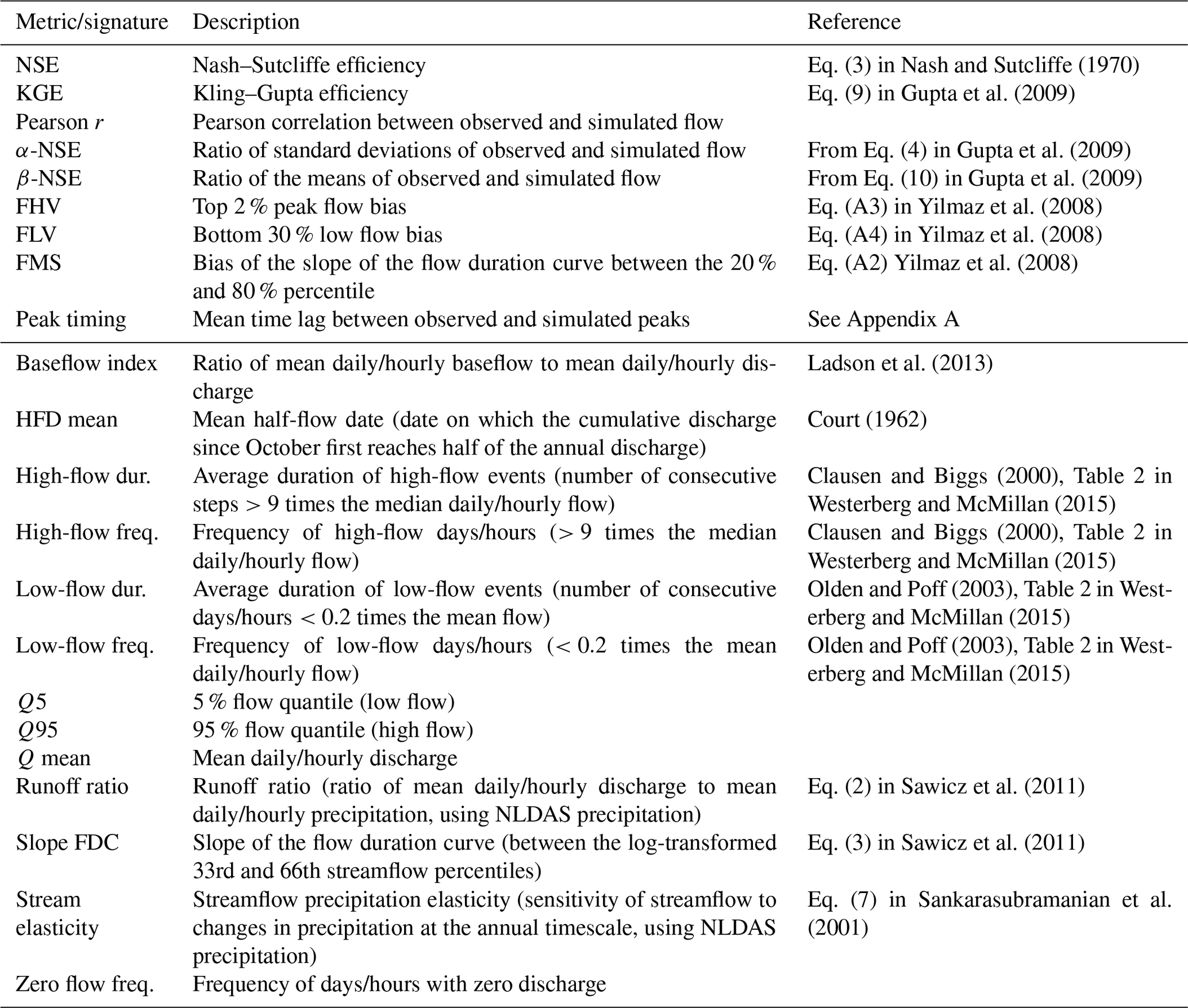
Nash and Sutcliffe (1970)Gupta et al. (2009)Gupta et al. (2009)Gupta et al. (2009)Yilmaz et al. (2008)Yilmaz et al. (2008)Yilmaz et al. (2008)Ladson et al. (2013)Court (1962)Clausen and Biggs (2000)Westerberg and McMillan (2015)Clausen and Biggs (2000)Westerberg and McMillan (2015)Olden and Poff (2003)Westerberg and McMillan (2015)Olden and Poff (2003)Westerberg and McMillan (2015)Sawicz et al. (2011)Sawicz et al. (2011)Sankarasubramanian et al. (2001)Table 3Evaluation metrics (upper table section) and hydrologic signatures (lower table section) used in this study. For each signature, we calculated the Pearson correlation between the signatures of observed and predicted discharge across all basins. Descriptions of the signatures are taken from Addor et al. (2018).
To quantify the cross-timescale consistency of the different models, we calculated the root mean squared deviation between daily predictions and hourly predictions when aggregated to daily values:
To account for randomness in LSTM weight initialization, all the LSTM results reported were calculated on hydrographs that result from averaging the predictions of 10 independently trained LSTM models. Each independently trained model used the same hyperparameters (bold values in Table D1), but a different random seed.
3.1 Benchmarking
Table 4 compares the median test period evaluation metrics of the MTS-LSTM and sMTS-LSTM architectures with the benchmark naive LSTM models and the process-based NWM. Figure 3 illustrates the cumulative distributions of per-basin NSE values of the different models. By this metric, all LSTM models, even the naive ones, outperformed the NWM at both hourly and daily time steps. All LSTM-based models performed slightly worse on hourly predictions than on daily predictions, an effect that was far more pronounced for the NWM. Accordingly, the results in Table 4 list differences in median NSE values between the NWM and the LSTM models ranging from 0.11 to 0.16 (daily) and around 0.19 (hourly). Among the LSTM models, differences between all metrics were comparatively small. The sMTS-LSTM achieved the best daily and hourly median NSE at both timescales. The naive models produced NSE values that were slightly lower, but the difference was not statistically significant at α=0.001 (Wilcoxon signed-rank test: (hourly), (daily)). The NSE distribution of the MTS-LSTM was significantly different from the sMTS-LSTM ( (hourly), (daily)), but the absolute difference was small. We leave it to the judgment of the reader to decide whether or not this difference is negligible from a hydrologic perspective.
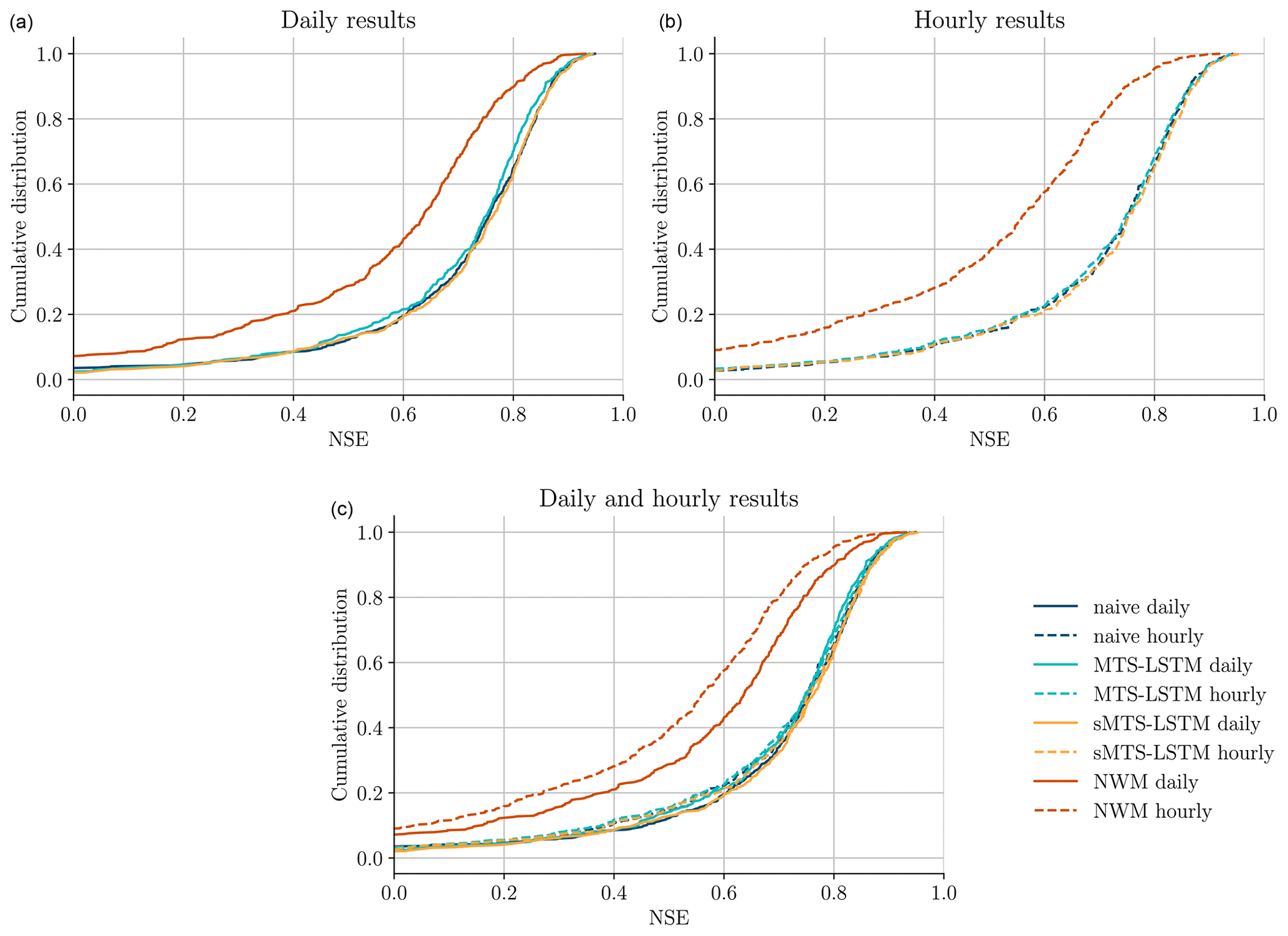
Figure 3Cumulative NSE distributions of the different models. Panel (a) (solid lines) shows NSEs of daily predictions, panel (b) (dashed lines) shows NSEs of hourly predictions, and panel (c) combines both plots into one for comparison.
All LSTM models exhibited lower peak-timing errors than the NWM. For hourly predictions, the median peak-timing error of the sMTS-LSTM was around 3.5 h, compared to more than 6 h for the NWM. Peak-timing errors for daily predictions are smaller values, since the error is measured in days instead of hours. The sMTS-LSTM yielded a median peak-timing error of 0.3 d, versus 0.5 d for the NWM. The process-based NWM, in turn, often produced results with better flow bias metrics, especially with respect to low flows (FLV). This agrees with prior work that indicates potential for improvement to deep learning models in arid climates (Kratzert et al., 2020; Frame et al., 2020). Similarly, the lower section of Table 4 lists correlations between hydrologic signatures of observed and predicted discharge: the NWM had the highest correlations for high-, low-, and zero-flow frequencies at both hourly and daily timescales, as well as for flow duration curve slopes at the hourly timescale.
Table 4Median metrics (upper table section) and Pearson correlation between signatures of observed and predicted discharge (lower table section) across all 516 basins for the sMTS-LSTM, MTS-LSTM, naive daily and hourly LSTMs, and the process-based NWM. Bold values highlight results that are not significantly different from the best model in the respective metric or signature (α=0.001). See Table 3 for a description of the metrics and signatures.
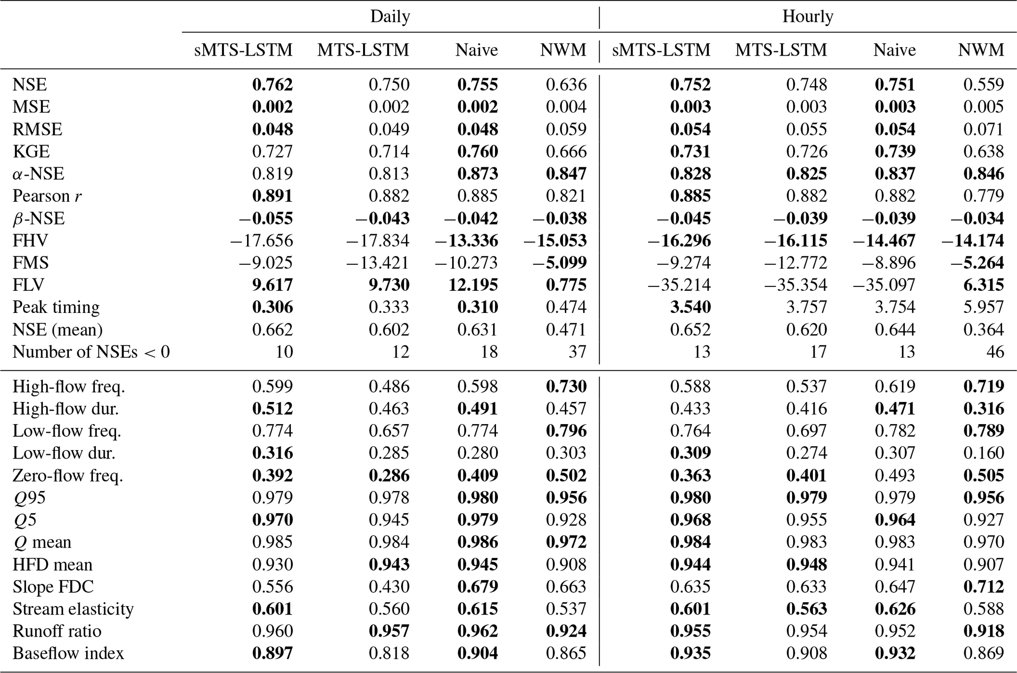
Figure 4 visualizes the distributions of NSE and peak-timing error across space for the hourly predictions with the sMTS-LSTM. As in previous studies, the NSE values are lowest in arid basins of the Great Plains and southwestern United States. The peak-timing error shows similar spatial patterns; however, the hourly peak-timing error also shows particularly high values along the southeastern coastline.
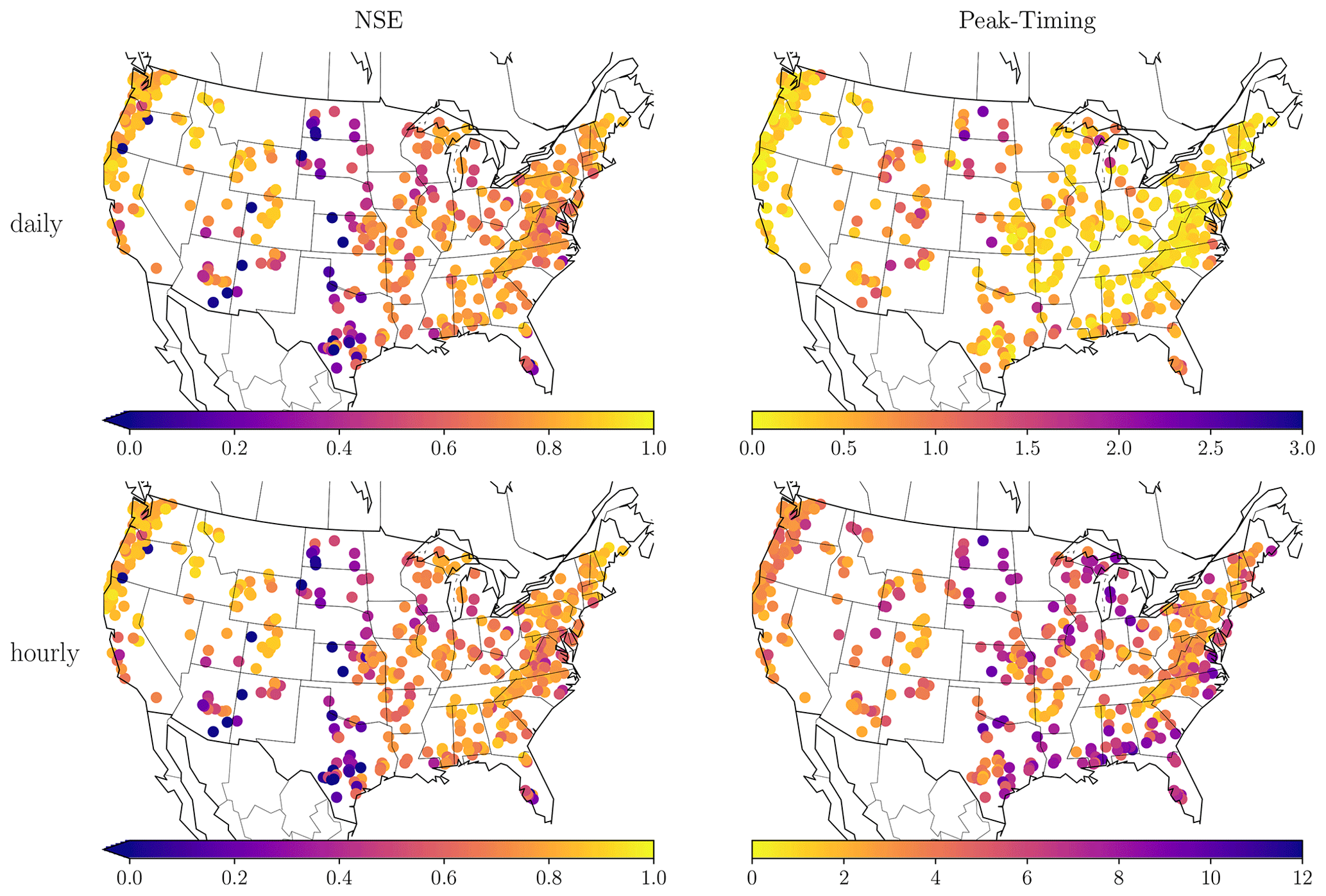
Figure 4NSE and peak-timing error by basin for daily and hourly sMTS-LSTM predictions. Brighter colors correspond to better values. Note the different color scales for daily and hourly peak-timing error.
3.2 Cross-timescale consistency
Since the (non-naive) LSTM-based models jointly predict discharge at multiple timescales, we can incentivize predictions that are consistent across timescales. As described in Sect. 2.3.2, this happens through a regularized NSE loss function that penalizes inconsistencies.
To gauge the effectiveness of this regularization, we compared inconsistencies between timescales in the best benchmark model, the sMTS-LSTM, with and without regularization. As a baseline, we also compared against the cross-timescale inconsistencies from two independent naive LSTMs. Table 5 lists the mean, median, and maximum root mean squared deviation between the daily predictions and the hourly predictions when aggregated to daily values. Without regularization, simultaneous prediction with the sMTS-LSTM yielded smaller inconsistencies than the naive approach (i.e., separate LSTMs at each timescale). Cross-timescale regularization further reduced inconsistencies and results in a median root mean squared deviation of 0.376 mm d−1.
Besides reducing inconsistencies, the regularization term appeared to have a small but beneficial influence on the overall skill of the daily predictions: with regularization, the median NSE increased slightly from 0.755 to 0.762. Judging from the hyperparameter tuning results, this appears to be a systematic improvement (rather than a fluke), because for both sMTS-LSTM and MTS-LSTM, at least the three best hyperparameter configurations used regularization.
Table 5Median and maximum root mean squared deviation (mm d−1) between daily and day-aggregated hourly predictions for the sMTS-LSTM with and without regularization, compared with independent prediction through naive LSTMs. p and d denote the significance (Wilcoxon signed-rank test) and effect size (Cohen’s d) of the difference to the inconsistencies of the regularized sMTS-LSTM.

3.3 Computational efficiency
In addition to differences in accuracy, the LSTM architectures have rather large differences in computational overhead and therefore runtime. The naive hourly model must iterate through 4320 input sequence steps for each prediction, whereas the MTS-LSTM and sMTS-LSTM only require 365 daily and 336 hourly steps. Consequently, where the naive hourly LSTM took more than one day to train on one NVIDIA V100 GPU, the MTS-LSTM and sMTS-LSTM took just over 6 (MTS-LSTM) and 8 h (sMTS-LSTM).
Moreover, while training is a one-time effort, the runtime advantage is even larger during inference: the naive model required around 9 h runtime to predict 10 years of hourly data for 516 basins on an NVIDIA V100 GPU. This is about 40 times slower than the MTS-LSTM and sMTS-LSTM models, which both required around 13 min for the same task on the same hardware – and the multi-timescale models generate daily predictions in addition to hourly ones.
3.4 Per-timescale input variables
While the MTS-LSTM yielded slightly worse predictions than the sMTS-LSTM in our benchmark evaluation, it has the important ability to ingest different input variables at each timescale. The following two experiments show how harnessing this feature can increase the accuracy of the MTS-LSTM beyond its shared version. In the first experiment, we used two daily input forcing sets (Daymet and Maurer) and one hourly forcing set (NLDAS). In the second experiment, we additionally ingested the daily forcings into the hourly LSTM branch.
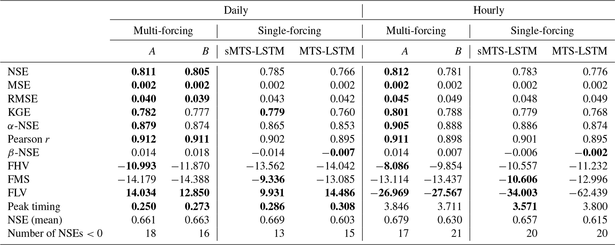
Table 6 compares the results of these two multi-forcings experiments with the single-forcing models (MTS-LSTM and sMTS-LSTM) from the benchmarking section. The second experiment – ingesting daily inputs into the hourly LSTM branch – yielded the best results. The addition of daily forcings increased the median daily NSE by 0.045 – from 0.766 to 0.811. Even though the hourly LSTM branch only obtains low-resolution additional values, the hourly NSE increased by 0.036 – from 0.776 to 0.812. This multi-input version of the MTS-LSTM was the best model in this study, significantly better than the best single-forcing model (sMTS-LSTM). An interesting observation is that it is daily inputs to the hourly LSTM branch that improved predictions. Using only hourly NLDAS forcings in the hourly branch, the hourly median NSE dropped to 0.781. Following Kratzert et al. (2020), we expect that additional hourly forcings datasets will have further positive impact on the hourly accuracy (beyond the improvement we see with additional daily forcings).
Table 6Median validation metrics across all 516 basins for the MTS-LSTMs trained on multiple sets of forcings (multi-forcing A uses daily Daymet and Maurer forcings as additional inputs into the hourly models, multi-forcing B uses just NLDAS as inputs into the hourly models). For comparison, the table shows the results for the single-forcing MTS-LSTM and sMTS-LSTM. Bold values highlight results that are not significantly different from the best model in the respective metric (α=0.001).
3.5 Predicting more timescales
In the above experiments, we evaluated models on daily and hourly predictions only. The MTS-LSTM architectures, however, generalize to other timescales.
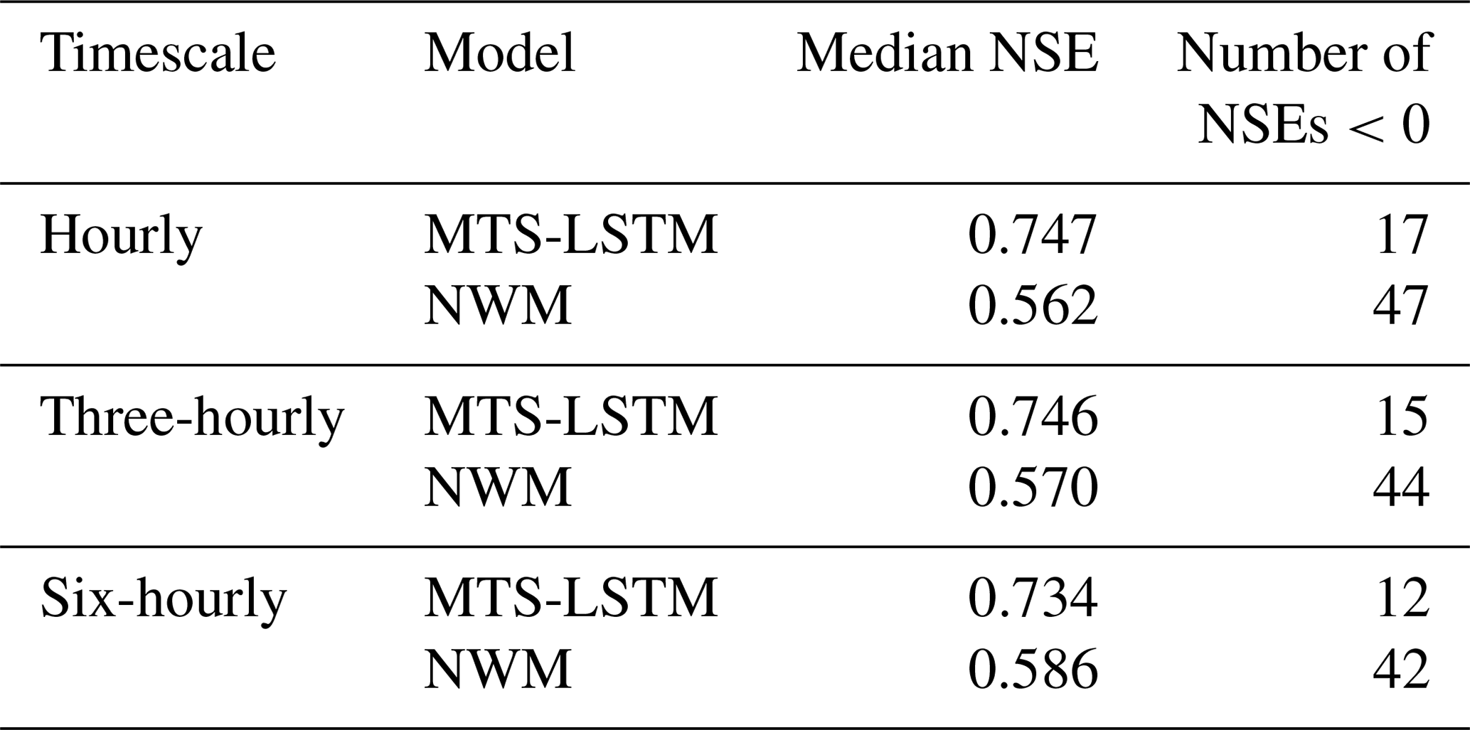
Table 7 lists the NSE values on the test period for each timescale. To calculate metrics, we considered only the first eight three-hourly and four six-hourly predictions that were made on each day. The hourly median NSE of 0.747 was barely different from the median NSE of the daily–hourly MTS-LSTM (0.748). While the three-hourly predictions were roughly as accurate as the hourly predictions, the six-hourly predictions were slightly worse (median NSE 0.734).
Table 7Median test period NSE and number of basins with NSE below zero across all 516 basins for NWM and the MTS-LSTM model trained to predict one-, three-, and six-hourly discharge. The three- and six-hourly NWM results are for aggregated hourly predictions.
The purpose of this work was to generalize LSTM-based rainfall–runoff modeling to multiple timescales. This task is not as trivial as simply running different deep learning models at different timescales due to long look-back periods, associated memory leaks, physical constraints between predictions at different time steps, and computational expense. With MTS-LSTM and sMTS-LSTM, we propose two LSTM-based rainfall–runoff models that make use of the specific (physical) nature of the simulation problem.
The results show that the advantage LSTMs have over process-based models on daily predictions (Kratzert et al., 2019) extends to sub-daily predictions. An architecturally simple approach, what we call the sMTS-LSTM, can process long-term dependencies at much smaller computational overhead than a naive hourly LSTM. Nevertheless, the high accuracy of the naive hourly model shows that LSTMs, even with a forget gate, can cope with very long input sequences. Additionally, LSTMs produce hourly predictions that are almost as good as their daily predictions, while the NWM's accuracy drops significantly from daily to hourly predictions. A more extensive hyperparameter tuning might even increase the accuracy of the naive model; however, this is difficult to test because of the large computational expense of training LSTMs with high-resolution input sequences that are long enough to capture all hydrologically relevant history.
The high quality of the sMTS-LSTM model indicates that the “summary” state between daily and hourly LSTM components contains as much information as the naive model extracts from the full hourly input sequence. This is an intuitive assumption, since watersheds are damped systems where the informative content of high-resolution forcings will almost certainly diminish at longer times in the past.
The MTS-LSTM adds the ability to use distinct sets of input variables for each timescale. This is an important feature for many operational use cases, as forcings with high temporal resolution often have shorter lead times than low-resolution products. In addition, per-timescale input variables allow for input data with lower temporal resolution, such as remote sensing products, without interpolation. Besides these conceptual considerations, this feature boosts model accuracy beyond the best single-forcings model, as we can ingest multiple forcing products at each timescale. Results from ingesting mixed input resolutions into the hourly LSTM branch (hourly NLDAS and daily Daymet and Maurer) highlight the flexibility of machine learning models and show that daily forcing histories can contain enough information to support hourly predictions. Yet, there remain a number of steps before these models can be truly operational:
-
First, like most academic rainfall–runoff models, our models operate in a reanalysis setting rather than performing actual lead-time forecasts.
-
Second, operational models predict other hydrologic variables in addition to streamflow. Hence, multi-objective optimization of LSTM water models is an open branch of future research.
-
Third, the implementation we use in this paper predicts more granular timescales only whenever it predicts a low-resolution step. At each low-resolution step, it predicts multiple high-resolution steps to offset the lower frequency. For instance, at daily and hourly target timescales, the LSTM predicts 24 hourly steps once a day. In a reanalysis setting, this does not matter, but in a forecasting setting, one needs to generate hourly predictions more often than daily predictions. Note, however, that this is merely a restriction of our implementation, not an architectural one: by allowing variable-length input sequences, we could produce one hourly prediction each hour (rather than 24 each day).
In future work, we see potential benefits in combining MTS-LSTM with approaches that incorporate further physical constraints into machine learning models (e.g., water balance; Hoedt et al., 2021). Further, it may be useful to extend our models such that they estimate uncertainty, as recently explored by Klotz et al. (2021), or to investigate architectures that pass information not just from coarse to fine timescales, but also vice versa. Our experimental architecture from Appendix B2 may serve as a starting point for such models.
This work represents one step toward developing operational hydrologic models based on deep learning. Overall, we believe that the MTS-LSTM is the most promising model for future use. It can integrate forcings of different temporal resolutions, generate accurate and consistent predictions at multiple timescales, and its computational overhead both during training and inference is far smaller than that of individual models per timescale.
Especially for predictions at high temporal resolutions, it is important that a model not only captures the correct magnitude of a flood event, but also its timing. We measure this with a “peak-timing” metric that quantifies the lag between observed and predicted peaks. First, we heuristically extract the most important peaks from the observed time series: starting with all observed peaks, we discard all peaks with topographic prominence smaller than the observed standard deviation and subsequently remove the smallest remaining peak until all peaks have a distance of at least 100 steps. Then, we search for the largest prediction within a window of one day (for hourly data) or three days (for daily data) around the observed peak. Given the pairs of observed and predicted peak time, the peak-timing error is their mean absolute difference.
Throughout our experiments, we found LSTMs to be a highly resilient architecture: we tried many different approaches to multi-timescale prediction, and a large fraction of them worked reasonably well, although not quite as well as the MTS-LSTM models presented in this paper. Nevertheless, we believe it makes sense to report some of these “negative” results – models that turned out not to work as well as the ones we finally settled on. Note, however, that the following reports are based on exploratory experiments with a few seeds and no extensive hyperparameter tuning.
B1 Delta prediction
Extending our final MTS-LSTM, we tried to facilitate hourly predictions for the LSTM by ingesting the corresponding day’s prediction into the hourly LSTM branch and only predicting each hour’s deviation from the daily mean. If anything, this approach slightly deteriorated the prediction accuracy (and made the architecture more complicated).
We then experimented with predicting 24 weights for each day that distribute the daily streamflow across the 24 h. This would have yielded the elegant side-effect of guaranteed consistency across timescales: the mean hourly prediction would always be equal to the daily prediction. Yet, the results were clearly worse, and, as we show in Sect. 3.2, we can achieve near-consistent results by incentive (regularization) rather than enforcement. One possible reason for the reduced accuracy is that it may be harder for the LSTM to learn two different things – predicting hourly weights and daily streamflow – than to predict the same streamflow at two timescales.
B2 Cross-timescale state exchange
Inspired by residual neural networks (ResNets) that use so-called skip connections to bypass layers of computation and allow for a better flow of gradients during training (He et al., 2016), we devised a “ResNet-multi-timescale LSTM” where after each day we combine the hidden state of the hourly LSTM branch with the hidden state of the daily branch into the initial daily and hourly hidden states for the next day. This way, we hoped, the daily LSTM branch might obtain more fine-grained information about the last few hours than it could infer from its daily inputs. While the daily NSE remained roughly the same, the hourly predictions in this approach became much worse.
B3 Multi-timescale input, single-timescale output
For both sMTS-LSTM and MTS-LSTM, we experimented with ingesting both daily and hourly data into the models, but only training them to predict hourly discharge. In this setup, the models could fully focus on hourly predictions rather than trying to satisfy two possibly conflicting goals. Interestingly, however, the hourly-only predictions were worse than the combined multi-timescale predictions. One reason for this effect may be that the state summary that the daily LSTM branch passes to the hourly branch is worse, as the model obtains no training signal for its daily outputs.
As mentioned in the introduction, the combination of ordinary differential equations (ODEs) and LSTMs presents another approach to multi-timescale prediction – one that is more accurately characterized as time-continuous prediction (as opposed to our multi-objective learning approach that predicts at arbitrary but fixed timescales). The ODE-LSTM passes each input time step through a normal LSTM, but then post-processes the resulting hidden state with an ODE that has its own learned weights. In effect, the ODE component can adjust the LSTM's hidden state to the time step size. We believe that our MTS-LSTM approach is better suited for operational streamflow prediction since ODE-LSTMs cannot directly process different input variables for different target timescales. That said, from a scientific standpoint, we think that the idea of training a model that can then generalize to arbitrary granularity is of interest (e.g., toward a more comprehensive and interpretable understanding of hydrologic processes).
Table C1Test period NSE for the MTS-LSTM and ODE-LSTM models trained on two and evaluated on three target timescales. (a) Training on daily and 12-hourly data, evaluation additionally on hourly predictions (hourly MTS-LSTM results obtained as 12-hourly predictions uniformly distributed across 12 h). (b) Training on hourly and three-hourly data, evaluation additionally on daily predictions (daily MTS-LSTM predictions obtained as averaged three-hourly values). The mean and median NSE are aggregated across the results for 10 basins; best values are highlighted in bold.
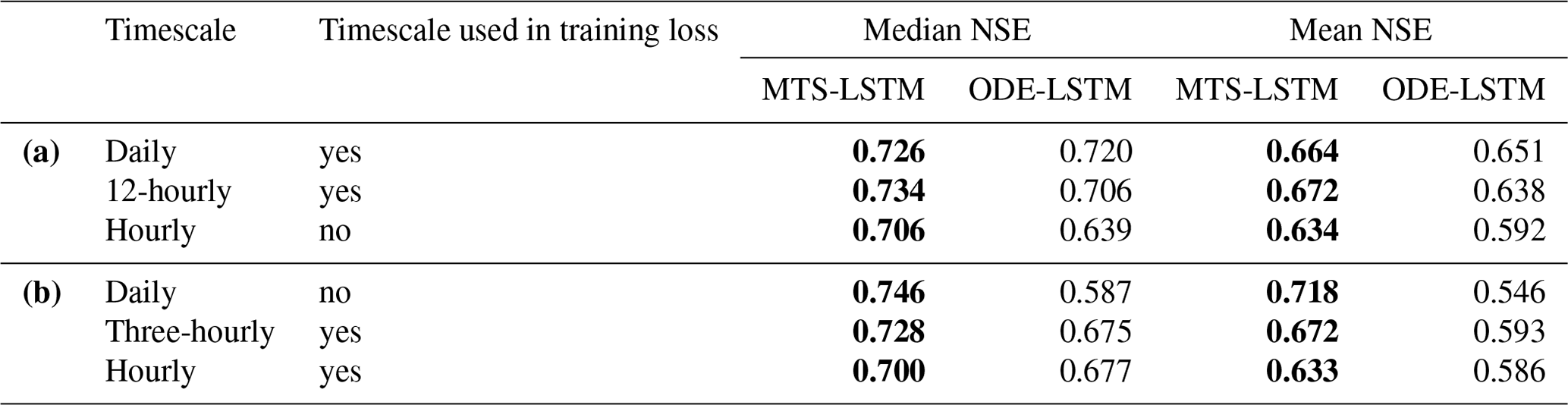
Although the idea of time-continuous predictions seemed promising, in our exploratory experiments it was better to use an MTS-LSTM and aggregate (or dis-aggregate) its predictions to the desired target temporal resolution. Note that due to the slow training of ODE-LSTMs, we carried out the following experiments on 10 basins (training one model per basin; we used smaller hidden sizes, higher learning rates, and trained for more epochs to adjust the LSTMs to this setting). Table C1 gives examples for predictions at untrained timescales. Table C1a shows the mean and median NSE values across the 10 basins when we trained the models on daily and 12-hourly target data but then generated hourly predictions (for the MTS-LSTM, we obtained hourly predictions by uniformly spreading the 12-hourly prediction across 12 h). Table C1b shows the results when we trained on hourly and three-hourly target data but then predicted daily values (for the MTS-LSTM, we aggregated eight three-hourly predictions into one daily time step). These initial results show that, in almost all cases, it is better to (dis-)aggregate MTS-LSTM predictions than to use an ODE-LSTM.
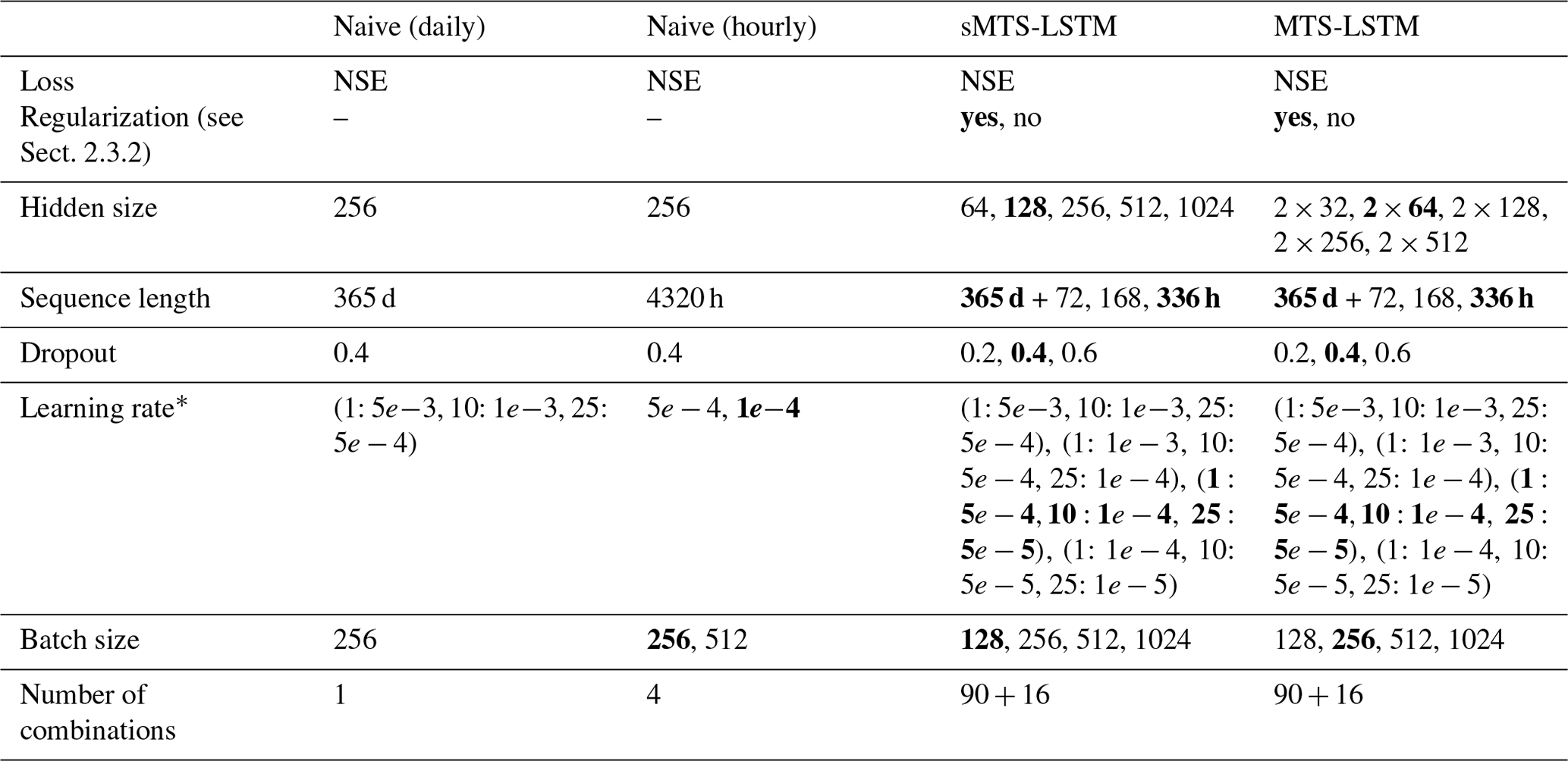
We performed a two-stage hyperparameter tuning for each of the multi-timescale models. In the first stage, we trained architectural model parameters (regularization, hidden size, sequence length, dropout) for 30 epochs at a batch size of 512 and a learning rate that starts at 0.001, reduces to 0.0005 after 10 epochs, and to 0.0001 after 20 epochs. We selected the configuration with the best median NSE (we considered the average of daily and hourly median NSE) and, in the second stage, tuned the learning rate and batch size. Table D1 lists the parameter combinations we explored.
We did not tune architectural parameters of the naive LSTM models, since the architecture has already been extensively tuned by Kratzert et al. (2019). The 24 times larger training set of the naive hourly model did, however, require additional tuning of learning rate and batch size, and we only trained for one epoch. As the extremely long input sequences greatly increase training time, we were only able to evaluate a relatively small parameter grid for the naive hourly model.
Table D1Hyperparameter tuning grid. The upper table section lists the architectural parameters tuned in stage one, the lower section lists the parameters tuned in stage two. In both stages, we trained three seeds for each parameter combination and averaged their NSEs. Bold values denote the best hyperparameter combination for each model.
* (1: r1, 5: r2, 10: r3, …) denotes a learning rate of r1 for epochs 1 to 4, of r2 for epochs 5 to 10, etc.
We trained all our machine learning models with the neuralhydrology Python library (https://doi.org/10.5281/zenodo.4688003, Kratzert et al., 2020).
All code to reproduce our models and analyses is available at https://doi.org/10.5281/zenodo.4687991 (Gauch, 2021).
The trained models and their predictions are available at https://doi.org/10.5281/zenodo.4071885 (Gauch et al., 2020a).
Hourly NLDAS forcings and observed streamflow are available at https://doi.org/10.5281/zenodo.4072700 (Gauch et al., 2020b).
The CAMELS static attributes are accessible at https://doi.org/10.5065/D6G73C3Q (Addor et al., 2017b). The CAMELS forcing data are accessible at https://ral.ucar.edu/sites/default/files/public/product-tool/camels-catchment-attributes-and-meteorology-for-large-sample-studies-dataset-downloads/basin_timeseries_v1p2_metForcing_obsFlow.zip (Newman et al., 2014b), however, the Maurer forcings distributed with this dataset should be replaced with their updated version available at https://doi.org/10.4211/hs.17c896843cf940339c3c3496d0c1c077 (Kratzert, 2019).
MG, FK, and DK designed all experiments. MG conducted all experiments and analyzed the results, together with FK and DK. GN supervised the manuscript from the hydrologic perspective, and JL and SH from the machine learning perspective. All authors worked on the manuscript.
The authors declare that they have no conflict of interest.
This research was undertaken thanks in part to funding from the Canada First Research Excellence Fund and the Global Water Futures Program, and enabled by computational resources provided by Compute Ontario and Compute Canada. We acknowledge the support of Microsoft Canada under the AI for Social Good program of the Waterloo Artificial Intelligence Institute. The ELLIS Unit Linz, the LIT AI Lab, and the Institute for Machine Learning are supported by the Federal State Upper Austria. We thank the projects AI-MOTION, DeepToxGen, AI-SNN, DeepFlood, Medical Cognitive Computing Center (MC3), PRIMAL, S3AI, DL for granular flow, ELISE (H2020-ICT-2019-3 ID: 951847), and AIDD. Further, we thank Janssen Pharmaceutica, UCB Biopharma SRL, Merck Healthcare KGaA, Audi.JKU Deep Learning Center, TGW LOGISTICS GROUP GMBH, Silicon Austria Labs (SAL), FILL Gesellschaft mbH, Anyline GmbH, Google (Faculty Research Award), ZF Friedrichshafen AG, Robert Bosch GmbH, Software Competence Center Hagenberg GmbH, TÜV Austria, and the NVIDIA Corporation.
This research has been supported by the Global Water Futures project, the Bundesministerium für Bildung, Wissenschaft und Forschung (grant nos. LIT-2018-6-YOU-212, LIT-2017-3-YOU-003, LIT-2018-6-YOU-214, and LIT-2019-8-YOU-213), the Österreichische Forschungsförderungsgesellschaft (grant nos. FFG-873979, FFG-872172, and FFG-871302), the European Commission's Horizon 2020 Framework Programme (AIDD (grant no. 956832)), Janssen Pharmaceuticals, UCB Biopharma SRL, the Merck Healthcare KGaA, the Audi.JKU Deep Learning Center, the TGW Logistics Group GmbH, Silicon Austria Labs (SAL), the FILL Gesellschaft mbH, the Anyline GmbH, Google, the ZF Friedrichshafen AG, the Robert Bosch GmbH, the Software Competence Center Hagenberg GmbH, TÜV Austria, the NVIDIA Corporation, and Microsoft Canada.
This paper was edited by Fabrizio Fenicia and reviewed by Thomas Lees and one anonymous referee.
Addor, N., Newman, A. J., Mizukami, N., and Clark, M. P.: The CAMELS data set: catchment attributes and meteorology for large-sample studies, Hydrol. Earth Syst. Sci., 21, 5293–5313, https://doi.org/10.5194/hess-21-5293-2017, 2017a. a
Addor, N., Newman, A., Mizukami, M., and Clark, M. P.: Catchment attributes for large-sample studies [data set], Boulder, CO, UCAR/NCAR, https://doi.org/10.5065/D6G73C3Q (last access: 14 April 2021), 2017. a
Addor, N., Nearing, G., Prieto, C., Newman, A. J., Le Vine, N., and Clark, M. P.: A Ranking of Hydrological Signatures Based on Their Predictability in Space, Water Resour. Res., 54, 8792–8812, https://doi.org/10.1029/2018WR022606, 2018. a, b
Araya, I. A., Valle, C., and Allende, H.: A Multi-Scale Model based on the Long Short-Term Memory for day ahead hourly wind speed forecasting, Pattern Recognition Letters, 136, 333–340, https://doi.org/10.1016/j.patrec.2019.10.011, 2019. a
Bengio, Y., Simard, P., and Frasconi, P.: Learning long-term dependencies with gradient descent is difficult, IEEE Transactions on Neural Networks, 5, 157–166, https://doi.org/10.1109/72.279181, 1994. a
Chung, J., Ahn, S., and Bengio, Y.: Hierarchical Multiscale Recurrent Neural Networks, arXiv preprint, arXiv:1609.01704, 2016. a
Clausen, B. and Biggs, B. J. F.: Flow variables for ecological studies in temperate streams: groupings based on covariance, J. Hydrol., 237, 184–197, https://doi.org/10.1016/S0022-1694(00)00306-1, 2000. a, b
Cosgrove, B. and Klemmer, C.: The National Water Model, available at: https://water.noaa.gov/about/nwm (last access: 25 January 2021), 2019. a, b
Court, A.: Measures of streamflow timing, J. Geophys. Res. (1896–1977), 67, 4335–4339, https://doi.org/10.1029/JZ067i011p04335, 1962. a
Frame, J., Nearing, G., Kratzert, F., and Rahman, M.: Post processing the U.S. National Water Model with a Long Short-Term Memory network, EarthArXiv, https://doi.org/10.31223/osf.io/4xhac, 2020. a
Gauch, M.: Code for “Rainfall-Runoff Prediction at Multiple Timescales with a Single Long Short-Term Memory Network”, Zenodo [code], https://doi.org/10.5281/zenodo.4687991 (last access: 14 April 2021), 2021. a
Gauch, M. and Lin, J.: A Data Scientist's Guide to Streamflow Prediction, arXiv preprint, arXiv:2006.12975, 2020. a
Gauch, M., Kratzert, F., Klotz, D., Nearing, G., Lin, J., and Hochreiter, S.: Models and Predictions for “Rainfall-Runoff Prediction at Multiple Timescales with a Single Long Short-Term Memory Network” [data set], Zenodo, https://doi.org/10.5281/zenodo.4095485, 2020a. a
Gauch, M., Kratzert, F., Klotz, D., Nearing, G., Lin, J., and Hochreiter, S.: Data for “Rainfall-Runoff Prediction at Multiple Timescales with a Single Long Short-Term Memory Network” [data set], Zenodo, https://doi.org/10.5281/zenodo.4072701, 2020b. a
Gers, F. A., Schmidhuber, J., and Cummins, F.: Learning to forget: continual prediction with LSTM, IET Conference Proceedings, pp. 850–855, 1999. a
Gochis, D. J., Barlage, M., Cabell, R., Casali, M., Dugger, A., FitzGerald, K., McAllister, M., McCreight, J., RafieeiNasab, A., Read, L., Sampson, K., Yates, D., and Zhang, Y.: The WRF-Hydro® modeling system technical description, available at: https://ral.ucar.edu/sites/default/files/public/projects/Technical%20Description%20%26amp%3B%20User%20Guides/wrfhydrov511technicaldescription.pdf (last access: 14 April 2021), 2020. a
Graves, A., Fernández, S., and Schmidhuber, J.: Multi-dimensional Recurrent Neural Networks, in: Artificial Neural Networks – ICANN 2007, edited by: de Sá, J. M., Alexandre, L. A., Duch, W., and Mandic, D., pp. 549–558, Springer Berlin Heidelberg, Berlin, Heidelberg, 2007. a
Greff, K., Srivastava, R. K., Koutník, J., Steunebrink, B. R., and Schmidhuber, J.: LSTM: A Search Space Odyssey, IEEE Transactions on Neural Networks and Learning Systems, 28, 2222–2232, https://doi.org/10.1109/TNNLS.2016.2582924, 2017. a
Gupta, H. V., Kling, H., Yilmaz, K. K., and Martinez, G. F.: Decomposition of the mean squared error and NSE performance criteria: implications for improving hydrological modelling, J. Hydrol., 377, 80–91, https://doi.org/10.1016/j.jhydrol.2009.08.003, 2009. a, b, c
He, K., Zhang, X., Ren, S., and Sun, J.: Deep Residual Learning for Image Recognition, in: Proceedings of the IEEE Conference on Computer Vision and Pattern Recognition (CVPR), June 2016, Las Vegas, Nevada, 770–778, 2016. a
Hochreiter, S. and Schmidhuber, J.: Long Short-Term Memory, Neural Computation, 9, 1735–1780, https://doi.org/10.1162/neco.1997.9.8.1735, 1997. a, b
Hoedt, P.-J., Kratzert, F., Klotz, D., Halmich, C., Holzleitner, M., Nearing, G., Hochreiter, S., and Klambauer, G.: MC-LSTM: Mass-Conserving LSTM, available at: https://arxiv.org/abs/2101.05186, 2021. a
Jozefowicz, R., Zaremba, W., and Sutskever, I.: An Empirical Exploration of Recurrent Network Architectures, in: Proceedings of the 32nd International Conference on Machine Learning, edited by: Bach, F. and Blei, D., vol. 37 of Proceedings of Machine Learning Research, pp. 2342–2350, PMLR, Lille, France, 2015. a, b
Klotz, D., Kratzert, F., Gauch, M., Keefe Sampson, A., Brandstetter, J., Klambauer, G., Hochreiter, S., and Nearing, G.: Uncertainty Estimation with Deep Learning for Rainfall–Runoff Modelling, Hydrol. Earth Syst. Sci. Discuss. [preprint], https://doi.org/10.5194/hess-2021-154, in review, 2021. a
Koutník, J., Greff, K., Gomez, F., and Schmidhuber, J.: A Clockwork RNN, arXiv preprint, arXiv:1402.3511, 2014. a
Kratzert, F., Klotz, D., Brenner, C., Schulz, K., and Herrnegger, M.: Rainfall–runoff modelling using Long Short-Term Memory (LSTM) networks, Hydrol. Earth Syst. Sci., 22, 6005–6022, https://doi.org/10.5194/hess-22-6005-2018, 2018. a
Kratzert, F., Gauch, M., and Klotz, D.: NeuralHydrology Python Library, Zenodo [code], https://doi.org/10.5281/zenodo.4688003 (last access: 14 April 2021), 2020. a
Kratzert, F.: CAMELS Extended Maurer Forcing Data, HydroShare [data set], https://doi.org/10.4211/hs.17c896843cf940339c3c3496d0c1c077 (last access: 14 April 2021), 2019. a
Kratzert, F., Klotz, D., Shalev, G., Klambauer, G., Hochreiter, S., and Nearing, G.: Towards learning universal, regional, and local hydrological behaviors via machine learning applied to large-sample datasets, Hydrol. Earth Syst. Sci., 23, 5089–5110, https://doi.org/10.5194/hess-23-5089-2019, 2019. a, b, c, d, e, f, g
Kratzert, F., Klotz, D., Hochreiter, S., and Nearing, G. S.: A note on leveraging synergy in multiple meteorological datasets with deep learning for rainfall-runoff modeling, Hydrol. Earth Syst. Sci. Discuss. [preprint], https://doi.org/10.5194/hess-2020-221, in review, 2020. a, b, c, d, e
Ladson, T. R., Brown, R., Neal, B., and Nathan, R.: A Standard Approach to Baseflow Separation Using The Lyne and Hollick Filter, Australasian J. Water Res., 17, 25–34, available at: https://www.tandfonline.com/doi/ref/10.7158/13241583.2013.11465417 (last access: 14 April 2021), 2013. a
Lechner, M. and Hasani, R.: Learning Long-Term Dependencies in Irregularly-Sampled Time Series, arXiv preprint, arXiv:2006.04418, 2020. a
Mozer, M.: Induction of Multiscale Temporal Structure, in: Advances in Neural Information Processing Systems 4, edited by: Moody, J. E., Hanson, S. J., and Lippmann, R., pp. 275–282, Morgan Kaufmann, 1991. a
Nash, J. E. and Sutcliffe, J. V.: River flow forecasting through conceptual models part I – A discussion of principles, J. Hydrol., 10, 282–290, https://doi.org/10.1016/0022-1694(70)90255-6, 1970. a
Neil, D., Pfeiffer, M., and Liu, S.-C.: Phased LSTM: Accelerating Recurrent Network Training for Long or Event-based Sequences, in: Advances in Neural Information Processing Systems 29, edited by: Lee, D. D., Sugiyama, M., Luxburg, U. V., Guyon, I., and Garnett, R., pp. 3882–3890, Curran Associates, Inc., 2016. a
Newman, A., Sampson, K., Clark, M. P., Bock, A., Viger, R., and Blodgett, D.: A large-sample watershed-scale hydrometeorological dataset for the contiguous USA, UCAR/NCAR [data set], https://doi.org/10.5065/d6mw2f4d, 2014. a, b
Newman, A., Sampson, K., Clark, M. P., Bock, A., Viger, R., and Blodgett, D.: CAMELS: Catchment Attributes and Meteorology for Large-sample Studies [data set], Boulder, CO, UCAR/NCAR, https://ral.ucar.edu/sites/default/files/public/product-tool/camels-catchment-attributes-and-meteorology-for-large-sample-studies-dataset-downloads/basin_timeseries_v1p2_metForcing_obsFlow.zip (last access: 14 April 2021), 2014. a
Newman, A., Mizukami, N., Clark, M. P., Wood, A. W., Nijssen, B., and Nearing, G.: Benchmarking of a Physically Based Hydrologic Model, J. Hydrometeorol., 18, 2215–2225, https://doi.org/10.1175/JHM-D-16-0284.1, 2017. a
Olah, C.: Understanding LSTM Networks, colah's blog, available at: https://colah.github.io/posts/2015-08-Understanding-LSTMs/ (last access: 14 April 2021), 2015. a
Olden, J. D. and Poff, N. L.: Redundancy and the choice of hydrologic indices for characterizing streamflow regimes, River Res. Appl., 19, 101–121, https://doi.org/10.1002/rra.700, 2003. a, b
Salas, F. R., Somos-Valenzuela, M. A., Dugger, A., Maidment, D. R., Gochis, D. J., David, C. H., Yu, W., Ding, D., Clark, E. P., and Noman, N.: Towards Real-Time Continental Scale Streamflow Simulation in Continuous and Discrete Space, J. Am. Water Resour. Assoc., 54, 7–27, https://doi.org/10.1111/1752-1688.12586, 2018. a, b
Sankarasubramanian, A., Vogel, R. M., and Limbrunner, J. F.: Climate elasticity of streamflow in the United States, Water Resour. Res., 37, 1771–1781, https://doi.org/10.1029/2000WR900330, 2001. a
Sawicz, K., Wagener, T., Sivapalan, M., Troch, P. A., and Carrillo, G.: Catchment classification: empirical analysis of hydrologic similarity based on catchment function in the eastern USA, Hydrol. Earth Syst. Sci., 15, 2895–2911, https://doi.org/10.5194/hess-15-2895-2011, 2011. a, b
Schmidhuber, J.: Neural Sequence Chunkers, Tech. rep. FKI 148 91, Technische Universität München, Institut für Informatik, 1991. a
United States Geological Survey: USGS Instantaneous Values Web Service, available at: https://waterservices.usgs.gov/rest/IV-Service.html (last access: 15 October 2020), 2021. a
Westerberg, I. K. and McMillan, H. K.: Uncertainty in hydrological signatures, Hydrol. Earth Syst. Sci., 19, 3951–3968, https://doi.org/10.5194/hess-19-3951-2015, 2015. a, b, c, d
Xia, Y., Mitchell, K., Ek, M., Sheffield, J., Cosgrove, B., Wood, E., Luo, L., Alonge, C., Wei, H., Meng, J., Livneh, B., Lettenmaier, D., Koren, V., Duan, Q., Mo, K., Fan, Y., and Mocko, D.: Continental-scale water and energy flux analysis and validation for the North American Land Data Assimilation System project phase 2 (NLDAS-2): 1. Intercomparison and application of model products, J. Geophys. Res.-Atmos., 117, D03109, https://doi.org/10.1029/2011JD016048, 2012. a, b
Yilmaz, K. K., Gupta, H. V., and Wagener, T.: A process-based diagnostic approach to model evaluation: Application to the NWS distributed hydrologic model, Water Resour. Res., 44, W09417, https://doi.org/10.1029/2007WR006716, 2008. a, b, c
Zamir, A. R., Sax, A., Cheerla, N., Suri, R., Cao, Z., Malik, J., and Guibas, L. J.: Robust Learning Through Cross-Task Consistency, in: The IEEE/CVF Conference on Computer Vision and Pattern Recognition (CVPR), June 2020 (online), 11197–11206, 2020. a
- Abstract
- Introduction
- Data and methods
- Results
- Discussion and Conclusion
- Appendix A: A peak-timing error metric
- Appendix B: Negative results
- Appendix C: Time-continuous prediction with ODE-LSTMs
- Appendix D: Hyperparameter tuning
- Code and data availability
- Author contributions
- Competing interests
- Acknowledgements
- Financial support
- Review statement
- References