the Creative Commons Attribution 4.0 License.
the Creative Commons Attribution 4.0 License.
 | 19 Mar 2021
Do small and large floods have the same drivers of change? A regional attribution analysis in Europe
Miriam Bertola
Alberto Viglione
Sergiy Vorogushyn
David Lun
Bruno Merz
Günter Blöschl
Recent studies have shown evidence of increasing and decreasing trends for average floods and flood quantiles across Europe. Studies attributing observed changes in flood peaks to their drivers have mostly focused on the average flood behaviour, without distinguishing small and large floods. This paper proposes a new framework for attributing flood changes to potential drivers, as a function of return period (T), in a regional context. We assume flood peaks to follow a non-stationary regional Gumbel distribution, where the median flood and the 100-year growth factor are used as parameters. They are allowed to vary in time and between catchments as a function of the drivers quantified by covariates. The elasticities of floods with respect to the drivers and the contributions of the drivers to flood changes are estimated by Bayesian inference. The prior distributions of the elasticities of flood quantiles to the drivers are estimated by hydrological reasoning and from the literature. The attribution model is applied to European flood and covariate data and aims at attributing the observed flood trend patterns to specific drivers for different return periods at the regional scale. We analyse flood discharge records from 2370 hydrometric stations in Europe over the period 1960–2010. Extreme precipitation, antecedent soil moisture and snowmelt are the potential drivers of flood change considered in this study. Results show that, in northwestern Europe, extreme precipitation mainly contributes to changes in both the median (q2) and 100-year flood (q100), while the contributions of antecedent soil moisture are of secondary importance. In southern Europe, both antecedent soil moisture and extreme precipitation contribute to flood changes, and their relative importance depends on the return period. Antecedent soil moisture is the main contributor to changes in q2, while the contributions of the two drivers to changes in larger floods (T>10 years) are comparable. In eastern Europe, snowmelt drives changes in both q2 and q100.
- Article
(13810 KB) - Full-text XML
- BibTeX
- EndNote


There is widespread concern that river flooding has become more frequent and severe during the last decades and that human-induced climate change and other drivers will further increase flood discharge and damage in many parts of the world (IPCC, 2012; Hirabayashi et al., 2013). This concern has given rise to a large number of studies investigating past changes in flood hazard, i.e. changes related to flood discharge, and flood risk, i.e. changes related to damage. The global pattern of increasing flood damage has been mainly attributed to increasing population, economic activities and assets in flood-prone areas (Bouwer, 2011; IPCC, 2012; Visser et al., 2014). In terms of changes in flood discharge, a variety of changes has been found (for shift in timing and trends in the magnitude of European floods, see Blöschl et al., 2017, 2019), and attempts to attribute detected changes have not resulted in a clear picture about the contribution of the underlying drivers (for a review on detecting and attributing flood hazard changes in Europe, see Hall et al., 2014).
The large majority of studies on past changes in flood hazard analysed the mean flood behaviour, using, for instance, the Mann–Kendall test to detect gradual changes or the Pettitt test for step changes in the mean or median annual flood (e.g. Petrow and Merz, 2009; Villarini et al., 2011; Mediero et al., 2014; Mangini et al., 2018). They implicitly assumed similar changes in different flood quantiles. This focus may be misleading, since changes in large floods may differ from those in the average behaviour. An illustrative example is the Mekong River, where studies found negative trends in the mean flood discharge, whereas the public perception suggested that the frequency of damaging floods had increased in the past decades. Delgado et al. (2010) resolved this mismatch by analysing the temporal change in flood discharge variability. They found an upward trend in interannual variability which outweighed the decreasing mean behaviour, leading to contrasting trends in the mean flood and rare floods. This change in flood variability could be attributed to changes in the Western Pacific monsoon (Delgado et al., 2012). Another recent example is the large-scale study of Bertola et al. (2020), which compared trends of small floods with those of large floods (i.e. the 2-year and the 100-year flood) across Europe. They found distinctive patterns of flood change which depend on the return period and catchment scale.
It has been widely acknowledged that drivers can affect small and large floods differently (e.g. Hall et al., 2014), and yet the focus has mainly been on changes in the mean flood behaviour. One reason for this may be the ability of quantifying changes in the mean more robustly than those of larger floods. However, both from theoretical and practical perspectives, detection and attribution of flood changes as a function of the return period are of considerable interest for understanding how the non-linearity in the hydrological system plays out and for providing guidance for flood risk management. The shape of the flood frequency curve and its changes in time are a reflection of the interplay between atmospheric processes and catchment state (soil moisture and snow), with different characteristics depending on the region, climate and runoff generation processes (Blöschl et al., 2013).
Rainfall itself may increase at different rates for small and extreme events in a changing climate. These changes may strongly differ depending on the region and season. In addition, changes in rainfall may be translated in a non-linear way into changes of various flood magnitudes due to the non-linearity of the catchment response. For example, Rogger et al. (2012) detected a change in the slope of the flood frequency curve and linked it to the interplay of catchment saturation and rainfall. Several studies indicated changes in precipitation amounts and intensities for different rainfall quantiles that might translate into different changes of small and large floods. For Germany, Murawski et al. (2016) found an increasing variability of precipitation along with increasing mean in seasons other than summer, which leads to a disproportional increase of heavy precipitation. Van den Besselaar et al. (2013) detected a decrease of the return period of extreme precipitation (5, 10 and 20 years) over Europe in the past 60 years between 2 % and 58 %. Berg et al. (2013) found a disproportional increase of high-intensity, convective precipitation with increasing temperature that goes beyond the Clausius–Clapeyron rate (7 % per degree of temperature increase) compared to low-intensity, stratiform precipitation. The review of a number of regional studies on past precipitation trends in Europe by Madsen et al. (2014) suggested a tendency for increasing extreme rainfalls. This trend seemed not to translate directly into positive trends in observed streamflow over large scales in Europe (Madsen et al., 2014). Similarly, Hodgkins et al. (2017) suggested that occurrence of floods with return periods of 25 to 100 years is dominated by multi-decadal climate variability rather than by long-term trends based on the analysis of more than 1200 gauges in Europe and North America. The study suggested that the occurrence rate of larger floods (50 and 100 years) increased slightly more strongly compared to smaller floods (25 years) in Europe over the past 50 years.
It has been observed that increases in precipitation extremes often do not translate into increasing floods (Madsen et al., 2014; Sharma et al., 2018). This is attributable to other factors which modulate flood response, such as initial soil moisture. For example, Tramblay et al. (2019) found that, despite the increase in extreme precipitation, the fewer detected annual occurrences of extreme floods in 171 Mediterranean basins were likely caused by decreasing soil moisture. The relationship between the flow rate and the initial saturation state of the soil is often non-linear, and the effect of antecedent soil moisture strongly depends on soil type and geology. The sensitivity of floods to initial soil moisture depends on flood magnitude, and runoff generation is more influential for smaller events. Vieux et al. (2009) analysed several watersheds in the Korean Peninsula with a distributed hydrologic model and found that the sensitivity of the watershed response to the initial degree of saturation is dependent on event magnitude. Zhu et al. (2018) simulated peak discharges for return periods of 2 to 500 years for several sub-watersheds in the Turkey River in the Midwestern United States and found that antecedent soil moisture modulates the role of rainfall structure in simulated flood response, particularly for smaller events. Grillakis et al. (2016) analysed flash flood events in two Greek catchments and one Austrian catchment and found higher sensitivity of the smallest flood events to initial soil moisture, compared to larger events. These results are consistent throughout the different regions and climates, confirming that the effects of initial soil moisture on flood response depend on flood magnitude.
Snow storage and snowmelt are other important factors that modulate flood response in temperate and cold regions. Snowmelt represents the dominant flood-generating process in northeastern Europe, and rain-on-snow is relevant for regions in central and northwestern Europe (Berghuijs et al., 2019; Kemter et al., 2020). It was observed that in catchments where snowmelt and rain-on-snow are the dominant flood-generating processes, the shape of the flood frequency curve is likely to flatten out at large return periods due to the upper limit of energy available for melt (Merz and Blöschl, 2003, 2008). Reduction in spring and summer snow cover extents has been detected as a result of increasing spring temperature in the Northern Hemisphere (Estilow et al., 2015). Several studies in regions dominated by snowmelt-induced peak flows reported a decrease in extreme streamflow and earlier spring snowmelt peak flows, likely caused by increasing temperature (Madsen et al., 2014). The effects of changing snow storage and snowmelt on the flood frequency curves likely depend on flood regimes and mixing of different flood-generating processes in the catchments. For example, in Carinthia, in the very south of Austria, the major floods tend to occur in autumn, and spring snowmelt floods represent a smaller fraction of events with small magnitude (Merz and Blöschl, 2003). Hence, changes in snow cover and snowmelt are expected to mainly affect the smaller floods in these climates. In contrast, in northeastern Europe, where snowmelt is the dominant flood-generating process of both small and large floods, the effects of decreasing snowmelt are likely important for the entire flood frequency curve.
Overall, the contributions of different drivers to flood changes as a function of return period are currently not well understood. This is partly due to detection and attribution studies focusing generally on the mean flood behaviour. Several studies applied non-stationary frequency analysis to attribute past flood changes to potential drivers. These studies typically allowed the parameters (often the location parameter) of the probability distribution of floods to vary in time, according to time-varying climatic covariates (e.g. Prosdocimi et al., 2014; Šraj et al., 2016; Steirou et al., 2019) and, more rarely, catchment and river covariates (e.g. López and Francés, 2013; Silva et al., 2017; Bertola et al., 2019). They attempted to identify and select covariates in the non-stationary model that provide a better fit to the flood data than the alternative stationary model. However, these studies aimed at attributing changes in the mean flood behaviour and did not explicitly separate the effects of drivers on floods associated with different return periods.
In this study we focus on flood quantiles in order to explicitly model the relationships between small and large floods (e.g. the 2-year and the 100-year flood) and potential drivers of flood change and to separate the effects of drivers on selected flood quantiles. For ease of interpretation, the quantiles are expressed here in terms of return periods, although alternative metrics are available under non-stationarity conditions (see, for example, Read and Vogel, 2015; Slater et al., 2020). We adopt a non-stationary flood frequency approach to attribute observed flood changes to potential drivers, used as covariates of the parameters of the regional probability distribution of floods. Extreme precipitation, antecedent soil moisture and snowmelt are the potential drivers considered. The relative contribution of the different drivers to flood changes is quantified through the elasticity of flood quantiles with respect to each driver.
The aim of this paper is to address two science questions: (a) is it possible to identify the relative contributions of different drivers to observed flood changes across Europe as a function of the return period, and if so, (b) what is the magnitude and sign of these contributions across Europe? Regarding the first question, one possible outcome is for the data to provide evidence that the relative contributions differ, or alternatively, the data may contain insufficient information to separate the effects by return period. Regarding the second question, the interest resides in understanding the relative importance of potential drivers as a function of return period, provided that such information can be inferred from the data.
2.1 Regional driver-informed model
In this study, we use non-stationary flood frequency analysis to attribute observed flood changes across Europe (see, for example, Blöschl et al., 2019; Bertola et al., 2020) to potential drivers, used as time-varying covariates. In the spirit of Bertola et al. (2020), we formulate the flood model as a regional Gumbel model. The Gumbel distribution has two parameters (i.e. the location μ and scale σ parameters), and its cumulative distribution function is
The two Gumbel parameters can be inferred from knowledge of two flood quantiles, for example, the 2-year and the 100-year flood. Flood quantiles q, associated with fixed annual exceedance probabilities 1−p, are expressed here in terms of return periods T, through . We adopt here the same alternative parameters as in Bertola et al. (2020), i.e. the 2-year flood q2 and the 100-year growth factor . The relationships linking q2 and to the Gumbel parameters are
where and .
The T-year flood can be obtained with the following relationship:
where , with y being the Gumbel reduced variate, which is related to the return period by
We adopt the following regional change model accounting for catchment area (S):
where X1, X2 and X3 are three covariates (i.e. time series of the potential drivers of flood change), and the α and γ terms represent regional model parameters to be estimated. The ε term, here assumed normally distributed, is a station-specific error term that accounts for additional local variability (i.e. not explained by catchment area and the covariates) of q2. Similar to the index flood method of Dalrymple (1960) and Hosking and Wallis (1997), we assume here that the growth curve is the same across all sites within the region (i.e. it depends on catchment area and the covariates only), while the median flood q2 (the index flood) is allowed to vary between sites, through the error term ε.
The elasticity of the generic flood quantile qT with respect to the covariate Xi is defined as
It represents the percentage change in qT, due to a 1 % change in Xi, i.e. how sensitive flood peaks are to changes in the drivers. However, the elasticity alone does not tell us how much the flood quantiles have actually changed (in time) due to observed changes of the drivers. Hence, we define the contribution of Xi to the changes in qT as
It represents the percentage change in qT due to the actual change in Xi. The total change in qT due to the changes in the drivers, assuming that the contributions are additive, is
A measure of relative contribution of Xi to the change in qT is expressed here by
where .
In the change model, the flood and covariate data are pooled and used simultaneously to attribute any observed changes in floods to their drivers. This pooling increases the robustness of the estimates (see, for example, Viglione et al., 2016) but requires an assumption of homogeneity. Specifically, we assume here that for a given return period and catchment scale, the elasticities of the flood discharges to their drivers are uniform within the region. We do allow the drivers to vary between catchments.
We frame the estimation problem in Bayesian terms through a Markov chain Monte Carlo (MCMC) approach, using the R package rStan (Carpenter et al., 2017), which makes use of a Hamiltonian Monte Carlo algorithm to sample the posterior distribution (Stan Development Team, 2018). For each inference, we generate four chains of 10 000 simulations each, with different initial values, and we check for their convergence. We use prior information on the model parameters to constrain their estimation to hydrologically plausible values (see Sect. 2.5).
2.2 Spatial correlation of floods
Spatial correlation of floods is not directly accounted for in the proposed regional change model of Sect. 2.1, and it may result in underestimated sample uncertainties (see, for example, Stedinger, 1983; Castellarin et al., 2008; Sun et al., 2014). Here, we adopt an approach proposed by Ribatet et al. (2012) and based on the work of Smith (1990), consisting in a magnitude adjustment to the likelihood function in a Bayesian framework, which accounts for the overall dependence in space and allows reliable credible intervals to be obtained. The adjusted likelihood is defined as
where L is the likelihood under the assumption of spatial independence, θ is the vector of unknown parameters and k is the magnitude adjustment factor to be estimated, such as (see Appendix A). The magnitude adjustment factor k represents the overall reduction of hydrological information in the data caused by the presence of spatial correlation and results in an inflated posterior variance of the parameters. If floods at different sites are spatially independent, k is 1; on the contrary, if floods are strongly cross-correlated, k assumes values close to 0. In this latter case, the sample uncertainty resulting from the adjusted likelihood will be larger, compared to the model in which spatial cross-correlation is not accounted for. For further details on the adjustment to the likelihood and its application to hydrological data, see Smith (1990), Ribatet et al. (2012) and Sharkey and Winter (2019).
2.3 Data
Consistent with Blöschl et al. (2019) and Bertola et al. (2020), we analyse long series of annual maximum discharges between 1960 and 2010, from 2370 hydrometric stations in 33 European countries (https://github.com/tuwhydro/europe_floods, last access: 9 April 2020). Stations affected by strong artificial alterations (such as large reservoirs in the proximity of the gauges) are not included in this database (Blöschl et al., 2019). The location of the stations is shown in Fig. 1. Their contributing catchment areas range from 5 to 100 000 km2, and the median record length is 51 years. The density of stations in the database is highest in central Europe and lowest in eastern and southern Europe, where time series are generally shorter (Fig. 1). The catchment boundaries relative to each hydrometric station are derived from the CCM River and Catchment Database (Vogt et al., 2007). Daily gridded precipitation and mean surface temperature are obtained from the E-OBS dataset (version 18.0e, resolution 0.1∘; Cornes et al., 2018). It covers the area 25–71.5∘ N × 25∘ W–45∘ E for the period 1950–2018.
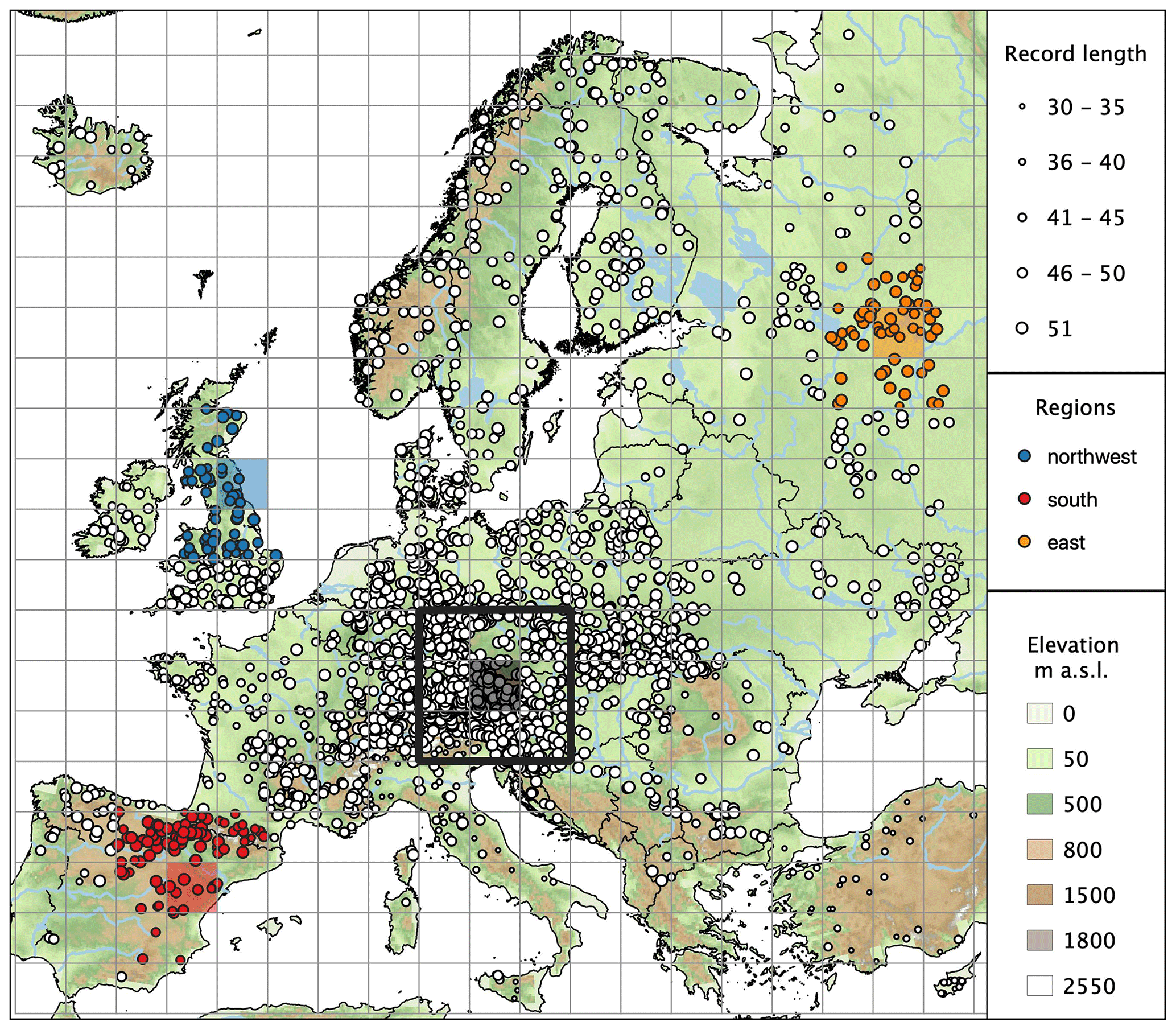
Figure 1Location of 2370 hydrometric stations in Europe and regions considered in this study. The size of the circles is proportional to the length of flood records. The grid size is 200 km. The black bordered region shows the size of the spatial moving windows analysed in Sect. 3.2. It consists of nine cells, corresponding to 600 km × 600 km, whose central cell is shaded black. Three regions analysed in Sect. 3.3, respectively located in northwestern, southern and eastern Europe, are shown with coloured circles, and the shaded regions represent their central cells.
2.4 Drivers of flood change
Because stations with substantial artificial alterations are not included in the database, in this study we consider three potential climatic drivers of flood change: (i) extreme precipitation, (ii) antecedent soil moisture and (iii) snowmelt. For each driver we obtain catchment-averaged time series, as described in detail in the following paragraphs, which are used as covariates in the regional model of Sect. 2.1. As the interest of this study resides in attributing flood changes to the long-term evolution of the drivers, we use average flood seasonality and its variability to identify time windows in which drivers are typically relevant for the generation of the annual peaks, rather than pairing floods with the corresponding event precipitation (which would be instead relevant for event attribution). Unlike in Viglione et al. (2016), scale dependence is here accounted for by the data, as we use local (i.e. catchment-averaged) covariates.
As in Bertola et al. (2019), this study aims at attributing flood changes to the long-term evolution of the covariates rather than their year-to-year variability. For this reason, we smooth the annual series of the drivers with the locally weighted polynomial regression LOESS (Cleveland, 1979) using the R function loess. The subset of data over which the local polynomial regression is performed is 10 years (i.e. 10 data-points of the series), and the degree of the local polynomials is set equal to 0, which is equivalent to a weighted 10-year moving average.
2.4.1 Extreme precipitation
Daily series of catchment-averaged precipitation between 1960 and 2010 are calculated for each hydrometric station from the daily gridded E-OBS precipitation and the catchment boundaries. For each station we identify a window around the average date of occurrence of floods , in which extreme precipitation is considered to be typically relevant for the generation of the annual peaks. The width of the window w is set between 90 and 360 d, and it is taken proportional to 1−R, with R being the concentration of the date of occurrence around the average date, through the following equation:
and R are obtained with circular statistics (see Appendix B). The window of dates is centred around , in a way that two-thirds of the window occur before the average date of occurrence of floods (as shown in Fig. 2 for an example series in one example year). For each year in the period of interest, we calculate the 7 d maximum precipitation within the identified window (which varies between catchments but is fixed between years).

Figure 2Procedure used to obtain the time series of extreme precipitation and antecedent soil moisture index. The figure shows the daily series of catchment-averaged precipitation for one example station in one example year. The thick dashed magenta line represents the average date of occurrence of annual floods for the example station, and the two thin dashed lines indicate the window of dates around the average date of occurrence, where extreme (7 d maximum) precipitation is selected (blue area). The respective preceding 30 d precipitation (green area) is representative of the antecedent soil moisture. The procedure is repeated for every year in the period of interest and every hydrometric station.
2.4.2 Antecedent soil moisture index
An index of antecedent soil moisture is obtained from daily catchment-averaged precipitation. For each year and each station, we calculate the 30 d precipitation preceding the 7 d window identified for extreme precipitation above. Longer temporal windows for antecedent precipitation have been assessed and did not result in significant differences in terms of long-term evolution and trend patterns of this driver, even for very large catchments. Other precipitation-based soil moisture indices are also available (e.g. the antecedent precipitation index, as defined in Woldemeskel and Sharma, 2016); however they require the definition of additional parameters and assumptions (e.g. lag and decay parameters). We use this index (for brevity, hereinafter referred to as “antecedent soil moisture”) based on precipitation instead of modelled soil moisture, as in Blöschl et al. (2019), in order to more strongly rely on observational data.
2.4.3 Snowmelt
Similar to precipitation, daily series of catchment-averaged temperature between 1960 and 2010 are obtained for each hydrometric station. We calculate daily series of catchment-averaged snowmelt according to a simple degree-day model (Parajka and Blöschl, 2008) as a function of mean daily air temperature TA and precipitation P:
where M and Ps are the daily snowmelt depth and snow water equivalent storage, DDF is the degree-day factor and Tm, TS and TR are the temperature thresholds that control the occurrence of melt, snow and rainfall, respectively. Here we assume C, C and DDF =2.5 mm per day per ∘C (Parajka and Blöschl, 2008; He et al., 2014). For each station, the time series of 7 d maximum snowmelt is obtained from daily snowmelt, using the same procedure illustrated above for the case of extreme precipitation.
2.5 Prior distributions of model parameters
In the attribution analysis we use informative priors of the parameters controlling the relationship between flood and covariate changes (i.e. the elasticities; see Eq. 6). This is done because we do not want to use the time patterns of the covariates Xi only to discriminate between drivers, which may lead to spurious correlations, but to “inform” the attribution analysis based on hydrological knowledge. Therefore, we set a priori constraints on the model parameters, based on qualitative reasoning and on prior literature. The changes in flood quantiles are expected to be caused by changes of the same sign in the drivers, given the covariates considered in this study (i.e. extreme precipitation, antecedent soil moisture and snowmelt). For example, increasing floods can be attributable to increasing extreme precipitation, while decreasing precipitation cannot reasonably cause increasing floods (which would correspond to a negative elasticity). In other words, we expect the elasticity of qT to Xi to be positive. For T=2 and 100 years, this translates respectively into
Eq. 13a represents the lower limit for the elasticity parameters of q2. The lower limit for is obtained from Eq. (13b) and depends on and on the growth factor:
For simplicity, we assume q100=2q2 as a reasonable approximation valid for Europe (Blöschl et al., 2013; Alfieri et al., 2015), and we simplify Eq. (14) to
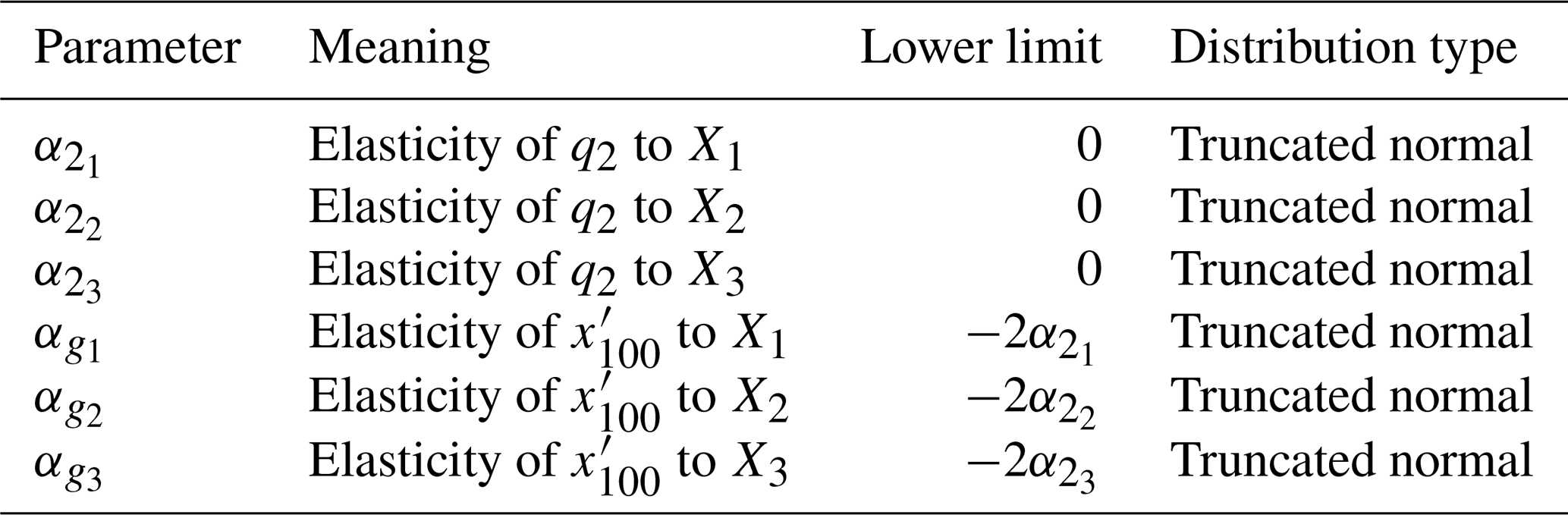
The prior distributions of and on are modelled as normal distributions 𝒩(0,2) with a truncated lower tail, as summarised in Table 1. For the remaining parameters, we set an improper uniform prior distribution.
Table 1Priors of model elasticity parameters controlling the relationship between flood and covariate changes.
2.6 Regional analyses
Following the spatial moving window approach of Bertola et al. (2020), we identify several regions of size 600 km × 600 km across Europe, which overlap by 200 km in both directions. We fit the regional flood change model of Sect. 2.1 to pooled flood and covariate data of sites within each region. The resulting 200 km × 200 km grid cells are shown in Fig. 1, and each of the considered regions is composed of nine adjacent cells, (e.g. the black bordered region in Fig. 1). All station-years contribute to the likelihood, and the likelihood is corrected using the magnitude adjustment to account for spatial cross-correlation between sites. The rationale behind the homogeneity assumption is that the spatial windows, given their size, are characterised by rather homogeneous climatic conditions relative to the overall variability within Europe.
In each region, we estimate the elasticity of q2 and q100 to the drivers Xi and the contribution of each driver to flood changes, obtained by multiplying the elasticity by the average driver trend in the region (Eq. 7). In regions where the average 7 d maximum snowmelt is less than 2 mm per day, only extreme precipitation and antecedent soil moisture are considered as potential drivers (i.e. Eq. 5 is modified by removing the contribution of X3). The resulting elasticity and contribution are plotted in the central 200 km × 200 km cell of the region (e.g. the shaded cell in the black bordered region in Fig. 1). The results are shown for a hypothetical catchment area S = 1000 km2, corresponding to a medium-sized catchment. This is because it is of interest to show average driver contributions to changes in flood quantiles within each region, rather than model results corresponding to an existing single catchment in the region. The attribution analysis is thereby performed at the regional scale, where average regional contributions of the decadal changes in the drivers to average regional trends in flood quantiles are estimated. The results of this analysis are shown in Sect. 3.2. In Sect. 3.3, the elasticities of flood quantiles to the drivers and their contributions to flood change are further analysed as a function of the return period, for three regions located respectively in northwestern, southern and eastern Europe (see Fig. 1).
3.1 Drivers of flood change
Time series of catchment-averaged (i) extreme precipitation, (ii) antecedent soil moisture and (iii) snowmelt are obtained for each hydrometric station for the period 1960–2010, as described in Sect. 2.4. Figure 3 shows maps of the mean value and the change of these drivers for each station in the period of interest. Extreme precipitation (Fig. 3a) exhibits its largest mean values in central and western Europe, particularly in the Alpine region and on the western Atlantic coast. Positive changes of extreme precipitation are observed in the Alpine region, northwestern and central Europe, Scandinavia and Poland; negative changes are observed in southern countries and in few spots in central Europe (Fig. 3d). Similar spatial patterns appear for antecedent soil moisture (Fig. 3b and e), but the negative changes tend to be more widespread and with stronger (negative) magnitude. Mean snowmelt is largest in northeastern Europe and in the Alpine region (Fig. 3c). Its changes are mostly negative across all Europe, with the exception of the very north and a few isolated spots (Fig. 3f).

Figure 3Mean value and change of catchment-averaged extreme precipitation (a, d), antecedent soil moisture (b, e) and snowmelt (c, f) for each station over the period 1960–2010.
3.2 Contributions of the drivers to flood change across Europe
The obtained time series of catchment-averaged extreme precipitation, antecedent soil moisture and snowmelt are used as covariates in the regional driver-informed model of Sect. 2.1. Figure 4 shows maps of the elasticity of the 2-year flood q2 and the 100-year flood q100 to each of the three drivers, as defined in Eq. (6), resulting from fitting the regional model to the pooled flood and covariate data in moving windows across Europe. The elasticities are measured here in percent per percent () and represent the percentage change in qT, due to a 1 % change in Xi, i.e. how sensitive flood peaks are to changes in the drivers. The value of the posterior median of the elasticities is shown together with the 90 % credible bounds, which represent a measure of the uncertainty associated with the estimate and take into account the different density of stations across Europe (i.e. larger uncertainties are typically observed in data-scarce regions).
The elasticity of q2 to extreme precipitation (Fig. 4a) is large (0.6 to 1.5) in western, central and southern Europe (indicating that the 2-year flood increases by 0.6 % to 1.5 % if extreme precipitation increases by 1 %), and lower values (0 to 0.25) are observed in northeastern Europe (i.e. the 2-year flood increases by 0 % to 0.25 % following a 1 % increase in extreme precipitation). Similar values of elasticity to extreme precipitation are observed for the 100-year flood across Europe (Fig. 4b), with small differences in northeastern Europe. This means that the elasticity of flood quantiles to extreme precipitation does not vary much with return period. In contrast, the elasticity of flood quantiles to soil moisture decreases with return period (i.e. q2 increases more than q100 if soil moisture increases by 1 %), and it is largest in southern Europe (0.25 to 0.6; Fig. 4b and 4e). Overall, the elasticities of q2 and q100 to soil moisture are smaller than those to extreme precipitation. The elasticity of floods to snowmelt is largest in northeastern Europe (Fig. 4c and d), where values above 1 are observed (i.e. a change of 1 % in snowmelt translates into a change in flood quantiles larger than 1 %). In northeastern Europe the elasticities of q2 and q100 to snowmelt are similar, while in central Europe and the Balkans they decrease with the return period.
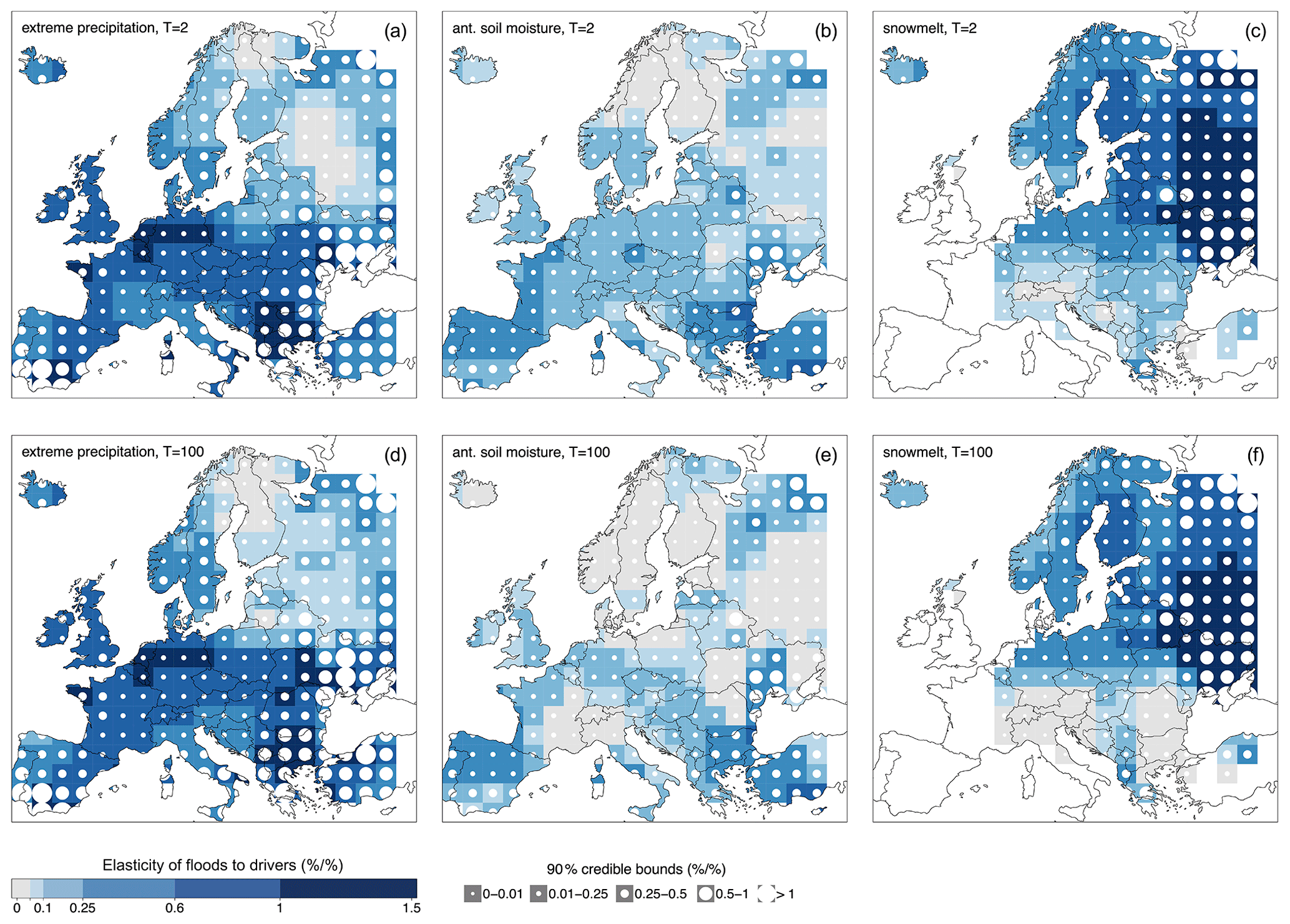
Figure 4Elasticity of the 2-year flood q2 (upper panels) and the 100-year flood q100 (lower panels) to extreme precipitation (a, d), antecedent soil moisture (b, e) and snowmelt (c, f). The median value of the posterior distribution of the elasticity is shown in each region with colours, and the size of the white circles is proportional to the respective 90 % credible bounds. The maps are shown for a hypothetical catchment area of 1000 km2
Figure 5 shows maps of the contributions of each of the three drivers to changes in q2 and q100, as defined in Eq. (7). They are obtained by multiplying the elasticities of flood quantiles to the drivers by the average changes (in percent per decade) in the drivers in each region over the period 1960–2010 (Eq. 7). They represent the change in flood quantiles, in percent per decade, caused by the change in a specific driver. Extreme precipitation (Fig. 5a and d) contributes to positive flood changes in northwestern and central Europe and to negative flood changes in southern and eastern Europe. The absolute value of the contributions of extreme precipitation appears to slightly decrease when moving from q2 to q100. Antecedent soil moisture contributes mostly to negative flood changes in southern Europe, and the magnitude of this contribution is smaller in absolute values for large floods than for the median floods (Fig. 5b and e). Snowmelt (Fig. 5c and f) contributes to marked negative changes in q2 and q100 in eastern Europe and to positive flood changes in northern Europe. We overall observe smaller contributions in absolute values to changes in q100 than q2. In data-scarce regions the credible bounds tend to be larger; i.e. the attribution results have larger uncertainties. Overall the uncertainties associated with the contribution of the drivers to changes in q100 do not seem to increase much compared to q2.
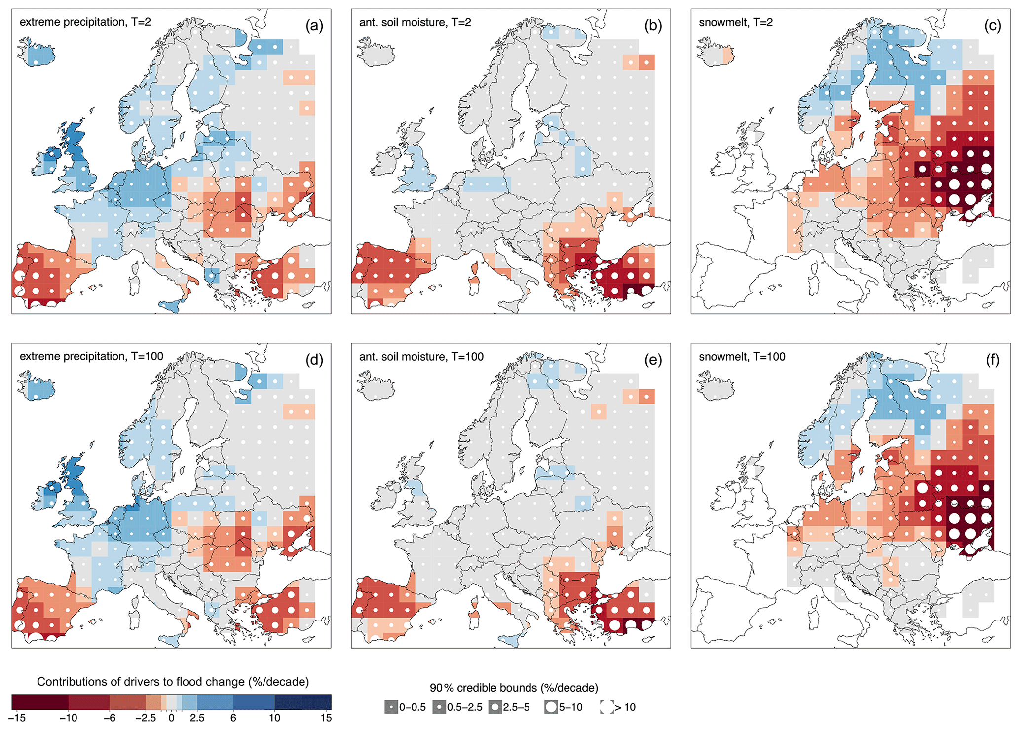
Figure 5Same as Fig. 4 but for contributions of extreme precipitation (a, d), antecedent soil moisture (b, e) and snowmelt (c, f) to changes in q2 and q100.
In order to further investigate the differences in terms of (absolute) contributions of the drivers to changes in large (i.e. q100) versus small floods (i.e. q2), we compute for each driver the ratio between these two quantities (Fig. 6). In the case of extreme precipitation (Fig. 6a), the ratio between its contributions to changes in q100 and q2 is between 0 and 1 in the Atlantic region, Spain, Italy, the Balkans, southern Germany, Austria and Finland; i.e. in these regions the contribution of extreme precipitation to changes in q100 is smaller, in absolute value, compared to changes in q2. In southern France, eastern Europe and Turkey, the opposite is observed (i.e. the ratio is larger than 1). Antecedent soil moisture and snowmelt generally contribute less to changes in q100 compared to q2 (i.e. the ratio is <1; Fig. 6b and c). Large uncertainties in the ratio of elasticities are observed in northeastern Europe, in the case of extreme precipitation and antecedent soil moisture (Fig. 6a and b), and in southern Europe, in the case of snowmelt (Fig. 6c). They result from values of the contribution of the drivers to q2 that are close to zero (see Fig. 5), indicating that, in these regions, flood changes are not explained by changes in extreme precipitation or antecedent soil moisture.
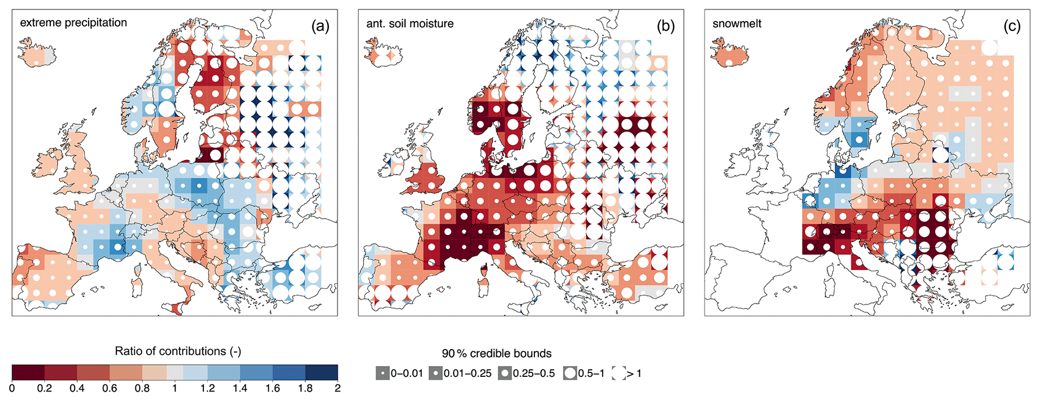
Figure 6Same as Fig. 4 but for the ratios of the contributions of extreme precipitation (a), antecedent soil moisture (b) and snowmelt (c) to changes in q100 relative to q2. Values below 1 (red colour) indicate that the contribution of the driver to q100 is smaller than the contribution to q2; values above 1 (blue colour) indicate that the contribution of the driver to q100 is larger than the contribution to q2.
Finally, for each region we obtain the relative contribution of the three drivers to changes in q2 and q100, as defined in Eq. (9) (Fig. 7). They represent the fraction of the regional trend in flood quantiles qT that is explained by changes in one driver. The relative contribution of extreme precipitation is the largest of all the drivers in most of western and central Europe for both q2 and q100 (Fig. 7a and d). The relative contribution is slightly smaller for large floods than for the median flood in northwestern Europe, while the opposite is the case in the south. In southern Europe antecedent soil moisture gives the largest relative contribution to changes in q2 (Fig. 7b), and its relative importance tends to decrease for more extreme floods (Fig. 7e). The relative contribution of snowmelt to flood changes clearly prevails over the other drivers in eastern Europe, with slightly decreasing strength for the higher return period.
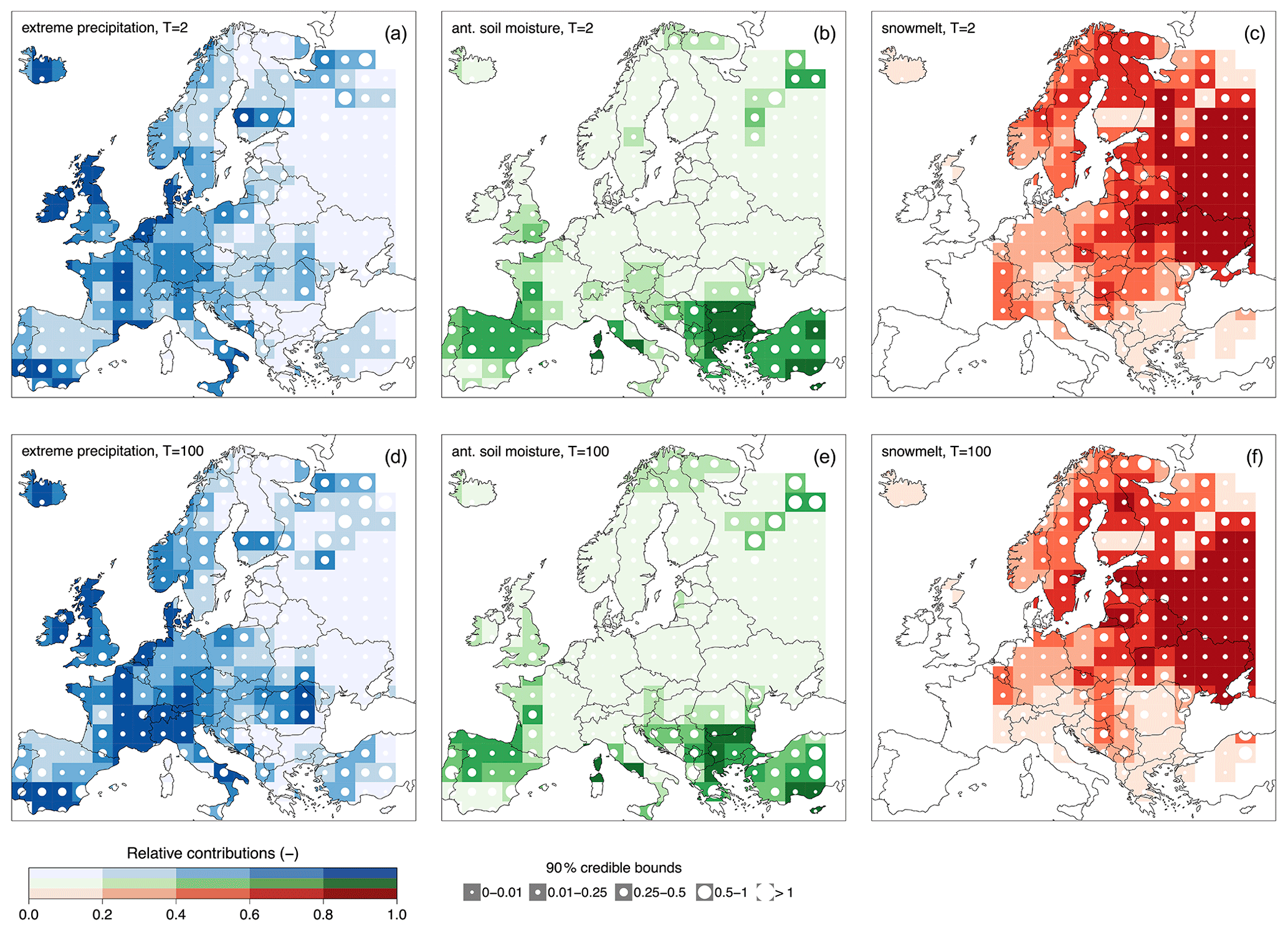
Figure 7Same as Fig. 4 but for relative contributions of extreme precipitation (a, d), antecedent soil moisture (b, e) and snowmelt (c, f) to changes in q2 and q100.
3.3 Contributions to flood change of the drivers in northwestern, southern and eastern Europe
In this section we select three example regions among those analysed in Sect. 3.2, located respectively in northwestern, southern and eastern Europe (see Fig. 1). For these three regions we further show in Fig. 8 the elasticities of floods to the drivers (first row), the contributions (second row) and relative contributions (third row) of the drivers to flood change, as a function of the return period. In the regions located in northwestern and southern Europe, snowmelt is excluded from the potential drivers as it does not represent a relevant process for most of the catchments in these regions (see Fig. 3c). Additionally, in Fig. 9, flood and driver time series are shown for the stations in each of the three regions, as well as their average changes in time within the regions.
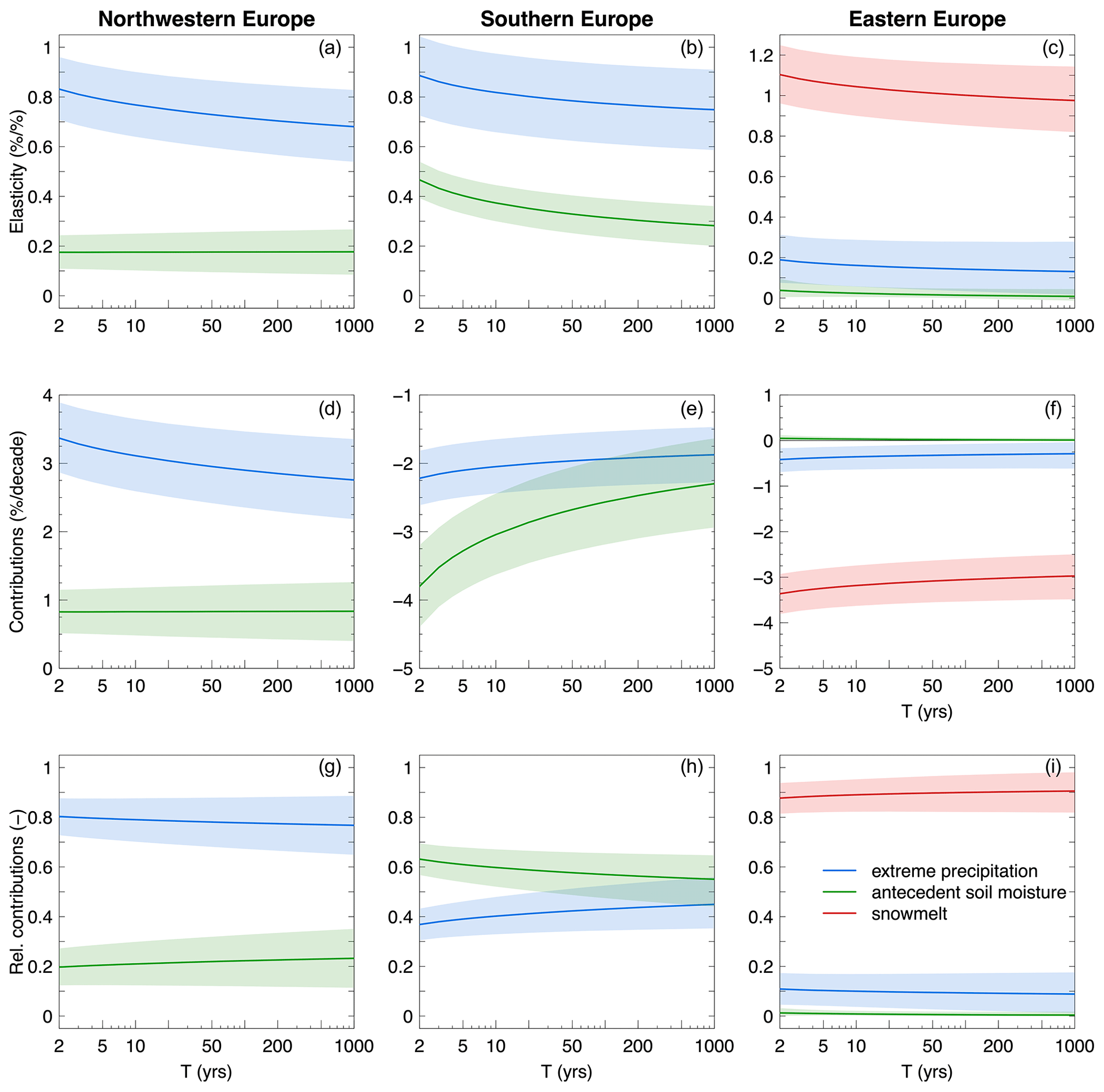
Figure 8Contributions of drivers to flood changes as a function of the return period in three regions (columns), respectively located in northwestern, southern and eastern Europe. Elasticity of floods to the drivers (a, b, c), contribution (d, e, f) and relative contribution (g, h, i) of the drivers to flood change are shown in the rows. The thick lines and the shaded areas represent the median and the 90 % credible intervals of their posterior distributions, respectively. The results are shown for a hypothetical catchment area of 1000 km2.
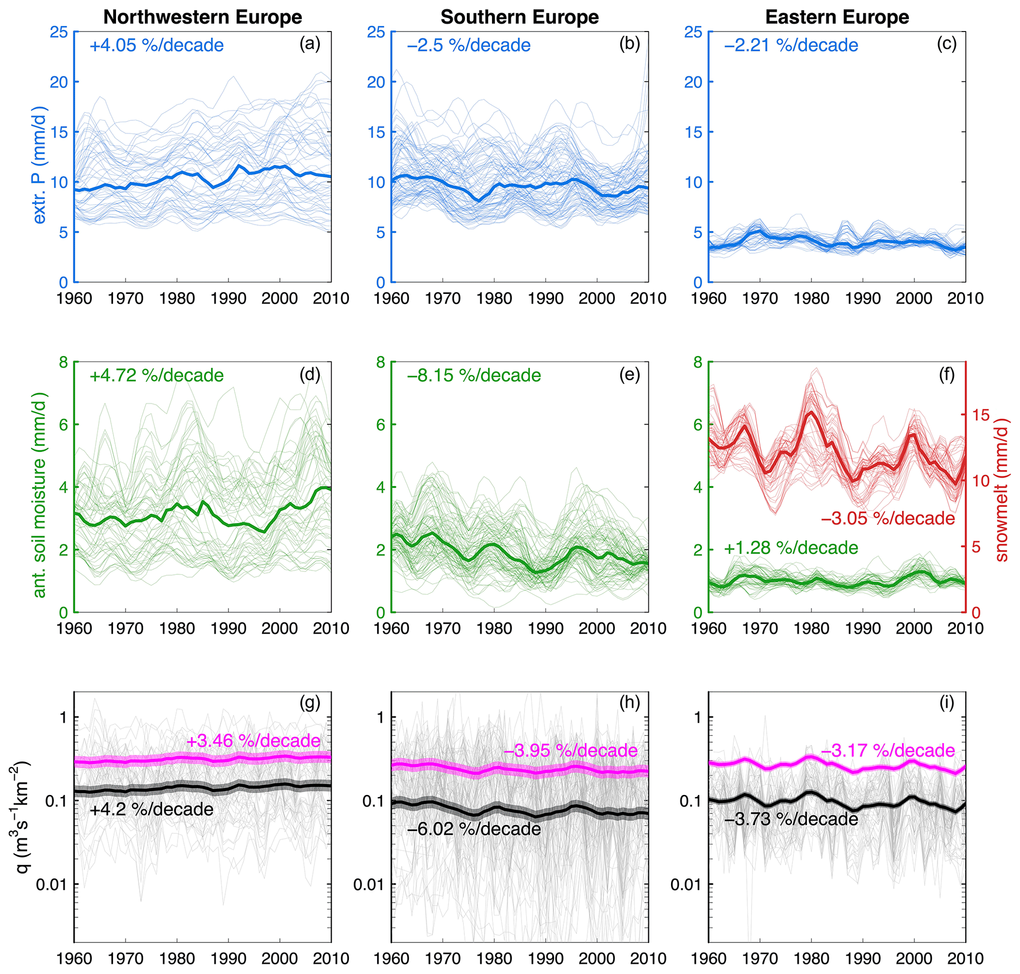
Figure 9Driver and flood time series in three regions, respectively located in northwestern, southern and eastern Europe. Thin lines represent flood and covariate time series for each station in the three regions. Thick lines in panels (a) to (f) represent the median. Thick lines in panels (g) to (i) represent the posterior median of the flood quantiles, and the shaded regions are the respective 90 % credible bounds. Numbers in panels (a) to (f) refer to the average changes in the drivers. Numbers in panels (g) to (i) refer to the sum of the contributions of the three drivers to changes in q2 (black) and q100 (magenta), i.e. to the average changes in q2 and q100 resulting from this model for S=1000 km2.
In the region in northwestern Europe, both extreme precipitation and antecedent soil moisture contribute to positive flood changes, with extreme precipitation representing the most important driver. Its contribution to flood trends decreases with increasing return period, while the contribution stays almost constant in the case of antecedent soil moisture (Fig. 8d and g). In the region in southern Europe extreme precipitation and antecedent soil moisture represent both important drivers. The elasticity of floods to extreme precipitation is larger than that to antecedent soil moisture (Fig. 8b). However, antecedent soil moisture contributes to a larger extent to negative flood changes for small return periods (i.e. T=2–10 years) due to larger (negative) changes in antecedent soil moisture (Fig. 9b and e). Its contribution decreases in absolute values with increasing return period (Fig. 8e). For more extreme events (T>10 years) the relative contribution of extreme precipitation increases and becomes comparable to that of antecedent soil moisture (Fig. 8h). The contribution of snowmelt to flood changes clearly dominates in the region located in eastern Europe at all return periods (Fig. 8c, f and i).
In this latter case, we observe that the posterior distribution of the elasticity of qT to antecedent soil moisture (representing the change in flood quantiles due to a 1 % change in the driver) is concentrated and flattened around zero. This results from the adopted informative priors of the elasticity parameters, which set their lower bound to zero, in order to exclude hydrologically implausible values (i.e. a negative elasticity would imply that decreasing floods are attributed to increasing antecedent soil moisture, or vice versa; see Sect. 2.5). In fact, antecedent soil moisture slightly increases over time in this region (Fig. 9f), while flood magnitude decreases for both T=2 and 100 years (Fig. 9i). As a consequence, the elasticity would tend to be negative (in case non-informative priors on the elasticity parameters are adopted), but it is constrained by the lower bound of the priors.
In this study, we attribute the changes in flood discharges that have occurred in Europe during the period 1960–2010 (Blöschl et al., 2019; Bertola et al., 2020) to potential drivers as a function of the return period, while previous detection and attribution studies have generally focused on the mean flood behaviour. In particular, we compare the relative contribution of extreme precipitation, antecedent soil moisture and snowmelt to changes in the median and the 100-year flood. The attribution study is framed in terms of a non-stationary flood frequency analysis, and the parameters of the distribution are estimated in a regional context with Bayesian inference. The study focuses on the average regional behaviour and flood attribution at the large scale. The results of the study should therefore be interpreted at the continental scale as average contributions of the drivers to flood changes in the regions, rather than at the catchment scale.
4.1 Is it possible to identify the relative contributions of different drivers to q100 changes as compared to q2 changes?
Our results suggest that in northwestern and eastern Europe, changes in small and large floods are driven mainly by one single driver, which dominates at all return periods. In northwestern Europe, extreme precipitation contributes to changes in both q2 and q100 for the most part, and the contribution of antecedent soil moisture is of secondary importance. Similarly, in eastern Europe, snowmelt clearly drives flood changes at all return periods. In southern Europe both antecedent soil moisture and extreme precipitation significantly contribute to flood changes, and their relative importance depends on the return period. Antecedent soil moisture contributes the most to changes in small floods (i.e. T=2–10 years), while the two drivers contribute with comparable magnitude to changes in more extreme events (T>10 years). Given the relative driver contributions and their credible bounds obtained in the analysis, the findings suggest that it is indeed possible to identify the relative contributions to changes in q2 and q100 with the presented approach.
4.2 What is the nature (sign and magnitude) of these contributions?
Extreme precipitation contributes to positive flood changes in northwestern Europe (about 3.3 % to 2.8 % per decade in Fig. 8), and its effect decreases slightly with return period in the region analysed in Sect. 3.3. In contrast, in the region selected in southern Europe, extreme precipitation contributes to 37 % to 45 % of the negative flood changes (corresponding to −2.2 % to −1.8 % per decade), depending on the return period. The contribution of antecedent soil moisture is negative in southern Europe and decreases in absolute value (from −3.8 % to −2.3 % per decade) with the return period in the analysed region. Finally, in eastern Europe snowmelt strongly contributes to negative flood changes in a similar way at all return periods (about −3 % per decade for the region in Sect. 3.3). This study more generally suggests that the changes in flood quantiles potentially caused by the three considered drivers are overall compatible, in terms of patterns and magnitude, with the flood changes observed in previous studies (Blöschl et al., 2019; Bertola et al., 2020). Some discrepancies are nevertheless observed, for instance, in Scandinavia, where the contributions of the drivers are all positive or close to zero, while mostly moderate negative flood trends were observed in previous studies. This discrepancy points to other drivers not accounted for in the presented model, such as river regulation effects (Arheimer and Lindström, 2019), or non-linear relationships between the drivers not captured by the model.
4.3 Discussion of model assumptions
One of the main assumptions in our analysis is that the three drivers (i.e. extreme precipitation, soil moisture and snowmelt) are the only candidates for explaining river flood changes. This selection is motivated by recent studies pointing out potential correlations between timing and magnitude of floods and the considered drivers across Europe (Blöschl et al., 2017, 2019; Berghuijs et al., 2019; Kemter et al., 2020). The effects of other drivers not accounted for in this study, such as land-cover change or river regulation, are probably not very large at the scale of Europe as we are focusing on catchments with minimum alteration. However, in contexts where anthropogenic alterations are important, it will be useful to extend the analysis for such effects. This attribution analysis may be repeated with catchment (e.g. land-use or land-cover changes) and river drivers (e.g. construction of reservoirs in the catchment) in addition to atmospheric covariates, if detailed information about changes in land use/land cover and river structures were available for European catchments and flood data of affected stations were collected.
In this study, we directly model the changes in flood quantiles because, in a Bayesian framework, it is typically easier for experts to formulate prior beliefs in terms of flood quantiles associated with large return periods, which they are familiar with, rather than in terms of distribution parameters (see, for example, the causal information expansion based on expert judgement in Viglione et al., 2013). Prior information on the elasticities is used in order to “inform” the attribution analysis, based on hydrological reasoning and the literature. Specifically, the prior distribution of the elasticities of q2 and q100 to the drivers is assumed positive. This is because any changes in the considered covariates are expected to translate into flood changes with the same sign. In practice, the prior distribution of the elasticity of q100 is reflected in a lower bounded prior distribution of the elasticity of the growth factor , which depends on the ratio between q100 and q2 (Sect. 2.5). For simplicity, we assume this ratio to be equal to 2. This assumption is reasonably valid for humid catchments (see, for example, Blöschl et al., 2013) and is in overall agreement with flood maps of the mean annual flood and q100 in Europe presented by Alfieri et al. (2015). However, in arid regions, larger values of this ratio (e.g. 4; see Blöschl et al., 2013) would be more appropriate (corresponding to stricter priors on the elasticity of the growth factor) because the flood frequency curves tend to be steeper.
The change model of Sect. 2.1 is fitted to the pooled flood and covariate data of several regions across Europe, where elasticities of flood quantiles to their drivers are assumed homogeneous. The rationale behind the homogeneity assumption is that the spatial windows, given their size, are characterised by rather homogeneous climatic conditions and presumably processes driving flood changes, relative to the overall variability within Europe. The attribution analysis is thereby performed at the regional scale, where average regional contributions of the decadal changes in the drivers to average regional trends in flood quantiles are estimated. Even though we have not assessed the statistical homogeneity of the regions in terms of the flood change model used here, we expect the effect of heterogeneity on the average regional behaviour to be less relevant than for the local behaviour. As already stated, the presented results should be interpreted at the European scale. Average driver contributions to changes in flood quantiles over the 5 analysed decades are presented, and this study does not aim at estimating driver contributions locally, in ungauged basins.
Spatial cross-correlation of floods at different sites is taken into account through an approach based on a magnitude adjustment to the likelihood. This results in larger uncertainties of the posterior distribution of the estimated parameters, compared to the case in which floods are considered spatially independent. Overall the obtained uncertainties associated with the contribution of the drivers to changes in q100 do not seem to increase much compared to q2, while a relevant increase would be reasonably expected. These results are valid under the assumption of the adopted model (i.e. Gumbel distribution), which may be too stringent. The model assumptions could be relaxed (e.g. adopting a generalised extreme value distribution) in order to allow for larger model flexibility.
This study represents a continental-scale attribution analysis and complements recent research on past changes in European floods by formally attributing the detected trends to potential drivers (i.e. extreme precipitation, antecedent soil moisture and snowmelt) as a function of return period. We propose a new data-based attribution approach to estimate driver contributions to changes in flood quantiles at the regional scale. This approach may be generalised and applied in other regions, where the explanation of past flood changes is of interest. The results show that in northwestern and eastern Europe, changes in both the 2-year and the 100-year flood are driven by a single driver only (i.e. respectively extreme precipitation and snowmelt), while in southern Europe, two drivers contribute to flood changes (i.e. soil moisture and extreme precipitation), with different relative contributions depending on the return period. The results of this study contribute to improved understanding of past flood changes across Europe over the past 5 decades.
Under the assumption of spatial independence of the data, the asymptotic distribution of the maximum likelihood estimator of the independence likelihood is , where θ0 is the true value of θ, and is the modified covariance matrix, where and . If the assumption of spatial independence is correct, we have H=V. In Sect. 2.2 we described an approach, proposed by Ribatet et al. (2012), that enables spatial cross-correlation to be accounted for in spatial datasets and consists in an overall adjustment to the likelihood. In this analysis we adopted a magnitude adjustment, through a factor k (Eq. 10). Ribatet et al. (2012) proposed to estimate k by setting
where p is the number of parameters in the independence likelihood, and λi are the eigenvalues of the matrix H−1V. The matrix H is approximated by the observed information matrix , and V is estimated by decomposing the likelihood into independent yearly contributions.
As in Blöschl et al. (2017), the average date of occurrence of floods and the concentration R of the date of occurrence around the average date are obtained with circular statistics, by conversion of the date of occurrence of a flood in the year i into an angular value Di:
with
where n is the number of peaks registered at that station, mi is the number of days in the year i and is the average number of days per year. When floods occur equally throughout the year, R=0, while R=1 when floods always occur on the same date.
The Stan code of the driver-informed model is available at https://github.com/MiriamBertola/flood_change_attribution (https://doi.org/10.5281/zenodo.4593140, Bertola et al., 2021).
The flood discharge data used in this paper can be obtained from the supplement of Blöschl et al. (2019) and are accessible at https://github.com/tuwhydro/europe_floods (Blöschl et al., 2019). Data regarding catchment areas belong to different institutions listed in Extended Data Table 1 in Blöschl et al. (2019). Catchment boundaries from the CCM River and Catchment database are available at https://ccm.jrc.ec.europa.eu/php/index.php?action=view&id=23 (Vogt et al., 2007). The E-OBS gridded precipitation and temperature dataset is available at https://www.ecad.eu/download/ensembles/download.php (Cornes et al., 2018).
All co-authors designed the overall study. MB performed the analysis and prepared the manuscript. All co-authors contributed to the interpretation of the results and writing of the paper.
The authors declare that they have no conflict of interest.
The authors would like to acknowledge funding from the European Union’s Horizon 2020 Research and Innovation Programme under the Marie Skłodowska-Curie grant agreement no. 676027, the FWF Vienna Doctoral Programme on Water Resource Systems (W1219-N28), the Austrian Science Funds (FWF) “SPATE” project I 3174 and the German Research Foundation (DFG; grant no. FOR 2416). We acknowledge the E-OBS dataset from the EU-FP6 project UERRA (http://www.uerra.eu, last access: 9 April 2020) and the Copernicus Climate Change Service and the data providers in the ECA&D project (https://www.ecad.eu, 9 April 2020). We would like to thank two anonymous reviewers and Louise Slater for their useful comments on the original version of the paper.
This research has been supported by the H2020 Marie Skłodowska-Curie Actions (grant no. 676027 – SYSTEM-RISK), the Austrian Science Fund (grant nos. W1219-N28 – Vienna Doctoral Programme on Water Resource Systems and I 3174 – SPATE) and the Deutsche Forschungsgemeinschaft (grant no. FOR 2416).
This paper was edited by Louise Slater and reviewed by two anonymous referees.
Alfieri, L., Burek, P., Feyen, L., and Forzieri, G.: Global warming increases the frequency of river floods in Europe, Hydrol. Earth Syst. Sci., 19, 2247–2260, https://doi.org/10.5194/hess-19-2247-2015, 2015. a, b
Arheimer, B. and Lindström, G.: Detecting Changes in River Flow Caused by Wildfires, Storms, Urbanization, Regulation, and Climate Across Sweden, Water Resour. Res., 55, 8990–9005, https://doi.org/10.1029/2019WR024759, 2019. a
Berg, P., Moseley, C., and Haerter, J. O.: Strong increase in convective precipitation in response to higher temperatures, Nat. Geosci., 6, 181–185, 2013. a
Berghuijs, W. R., Harrigan, S., Molnar, P., Slater, L. J., and Kirchner, J. W.: The Relative Importance of Different Flood-Generating Mechanisms Across Europe, Water Resour. Res., 55, 4582–4593, https://doi.org/10.1029/2019WR024841, 2019. a, b
Bertola, M., Viglione, A., and Blöschl, G.: Informed attribution of flood changes to decadal variation of atmospheric, catchment and river drivers in Upper Austria, J. Hydrol., 577, 123919, https://doi.org/10.1016/j.jhydrol.2019.123919, 2019. a, b
Bertola, M., Viglione, A., Lun, D., Hall, J., and Blöschl, G.: Flood trends in Europe: are changes in small and big floods different?, Hydrol. Earth Syst. Sci., 24, 1805–1822, https://doi.org/10.5194/hess-24-1805-2020, 2020. a, b, c, d, e, f, g, h
Bertola, M., Viglione, A., Vorogushyn, S., Lun, D., Merz, B., and Blöschl, G.: MiriamBertola/flood_change_attribution: Stan code for flood change attribution v1.0 (Version v1.0), Zenodo, https://doi.org/10.5281/zenodo.4593140, 2021. a
Blöschl, G., Sivapalan, M., Wagener, T., Viglione, A., and Savenije, H.: Runoff Prediction in Ungauged Basins: Synthesis across Processes, Places and Scales, Cambridge University Press, Cambridge, United Kingdom, https://doi.org/10.1017/CBO9781139235761, 2013. a, b, c, d
Blöschl, G., Hall, J., Parajka, J., Perdigão, R. A. P., Merz, B., Arheimer, B., Aronica, G. T., Bilibashi, A., Bonacci, O., Borga, M., Čanjevac, I., Castellarin, A., Chirico, G. B., Claps, P., Fiala, K., Frolova, N., Gorbachova, L., Gül, A., Hannaford, J., Harrigan, S., Kireeva, M., Kiss, A., Kjeldsen, T. R., Kohnová, S., Koskela, J. J., Ledvinka, O., Macdonald, N., Mavrova-Guirguinova, M., Mediero, L., Merz, R., Molnar, P., Montanari, A., Murphy, C., Osuch, M., Ovcharuk, V., Radevski, I., Rogger, M., Salinas, J. L., Sauquet, E., Šraj, M., Szolgay, J., Viglione, A., Volpi, E., Wilson, D., Zaimi, K., and Živković, N.: Changing climate shifts timing of European floods, Science, 357, 588–590, https://doi.org/10.1126/science.aan2506, 2017. a, b, c
Blöschl, G., Hall, J., Parajka, J., Perdigão, R. A. P., Merz, B., Arheimer, B., Aronica, G. T., Bilibashi, A., Bonacci, O., Borga, M., Čanjevac, I., Castellarin, A., Chirico, G. B., Claps, P., Fiala, K., Frolova, N., Gorbachova, L., Gül, A., Hannaford, J., Harrigan, S., Kireeva, M., Kiss, A., Kjeldsen, T. R., Kohnová, S., Koskela, J. J., Ledvinka, O., Macdonald, N., Mavrova-Guirguinova, M., Mediero, L., Merz, R., Molnar, P., Montanari, A., Murphy, C., Osuch, M., Ovcharuk, V., Radevski, I., Rogger, M., Salinas, J. L., Sauquet, E., Šraj, M., Szolgay, J., Viglione, A., Volpi, E., Wilson, D., Zaimi, K., and Živković, N.: Changing climate both increases and decreases European river floods, Nature, 573, 108–111, https://doi.org/10.1038/s41586-019-1495-6, 2019 (data available at: https://github.com/tuwhydro/europe_floods, last access: 9 April 2020). a, b, c, d, e, f, g, h, i, j, k
Bouwer, L. M.: Have disaster losses increased due to anthropogenic climate change?, B. Am. Meteorol. Soc., 92, 39–46, 2011. a
Carpenter, B., Gelman, A., Hoffman, M., Lee, D., Goodrich, B., Betancourt, M., Brubaker, M., Guo, J., Li, P., and Riddell, A.: Stan: A Probabilistic Programming Language, J. Stat. Softw., 76, 1–32, https://doi.org/10.18637/jss.v076.i01, 2017. a
Castellarin, A., Burn, D., and Brath, A.: Homogeneity testing: How homogeneous do heterogeneous cross-correlated regions seem?, J. Hydrol., 360, 67–76, https://doi.org/10.1016/j.jhydrol.2008.07.014, 2008. a
Cleveland, W. S.: Robust Locally Weighted Regression and Smoothing Scatterplots, J. Am. Stat. Assoc., 74, 829–836, https://doi.org/10.1080/01621459.1979.10481038, 1979. a
Cornes, R. C., van der Schrier, G., van den Besselaar, E. J., and Jones, P. D.: An Ensemble Version of the E-OBS Temperature and Precipitation Data Sets, J. Geophys. Res.-Atmos., 123, 9391–9409, https://doi.org/10.1029/2017JD028200, 2018 (data available at: https://www.ecad.eu/download/ensembles/download.php, last access: 9 April 2020). a, b
Dalrymple, T.: Flood frequency methods, US geological survey, Water Supply Paper A, 1543, 11–51, 1960. a
Delgado, J. M., Merz, B., and Apel, H.: A climate-flood link for the lower Mekong River, Hydrol. Earth Syst. Sci., 16, 1533–1541, https://doi.org/10.5194/hess-16-1533-2012, 2012. a
Delgado, J. M., Apel, H., and Merz, B.: Flood trends and variability in the Mekong river, Hydrol. Earth Syst. Sci., 14, 407–418, https://doi.org/10.5194/hess-14-407-2010, 2010. a
Estilow, T. W., Young, A. H., and Robinson, D. A.: A long-term Northern Hemisphere snow cover extent data record for climate studies and monitoring, Earth Syst. Sci. Data, 7, 137–142, https://doi.org/10.5194/essd-7-137-2015, 2015. a
Grillakis, M., Koutroulis, A., Komma, J., Tsanis, I., Wagner, W., and Blöschl, G.: Initial soil moisture effects on flash flood generation – A comparison between basins of contrasting hydro-climatic conditions, J. Hydrol., 541, 206–217, https://doi.org/10.1016/j.jhydrol.2016.03.007, 2016. a
Hall, J., Arheimer, B., Borga, M., Brázdil, R., Claps, P., Kiss, A., Kjeldsen, T. R., Kriaučiūnienė, J., Kundzewicz, Z. W., Lang, M., Llasat, M. C., Macdonald, N., McIntyre, N., Mediero, L., Merz, B., Merz, R., Molnar, P., Montanari, A., Neuhold, C., Parajka, J., Perdigão, R. A. P., Plavcová, L., Rogger, M., Salinas, J. L., Sauquet, E., Schär, C., Szolgay, J., Viglione, A., and Blöschl, G.: Understanding flood regime changes in Europe: a state-of-the-art assessment, Hydrol. Earth Syst. Sci., 18, 2735–2772, https://doi.org/10.5194/hess-18-2735-2014, 2014. a, b
He, Z. H., Parajka, J., Tian, F. Q., and Blöschl, G.: Estimating degree-day factors from MODIS for snowmelt runoff modeling, Hydrol. Earth Syst. Sci., 18, 4773–4789, https://doi.org/10.5194/hess-18-4773-2014, 2014. a
Hirabayashi, Y., Mahendran, R., Koirala, S., Konoshima, L., Yamazaki, D., Watanabe, S., Kim, H., and Kanae, S.: Global flood risk under climate change, Nat. Clim. Change, 3, 816–821, 2013. a
Hodgkins, G. A., Whitfield, P. H., Burn, D. H., Hannaford, J., Renard, B., Stahl, K., Fleig, A. K., Madsen, H., Mediero, L., Korhonen, J., Murphy, C., and Wilson, D.: Climate-driven variability in the occurrence of major floods across North America and Europe, J. Hydrol., 552, 704–717, 2017. a
Hosking, J. and Wallis, J. R.: Regional Frequency Analysis, Regional Frequency Analysis, Cambridge University Press, Cambridge, UK, 240 pp., 1997. a
IPCC: IPCC, 2012: Managing the Risks of Extreme Events and Disasters to Advance Climate Change Adaptation. A Special Report of Working Groups I and II of the Intergovernmental Panel on Climate Change, Cambridge University Press, Cambridge, United Kingdom and New York, NY, USA, 2012. a, b
Kemter, M., Merz, B., Marwan, N., Vorogushyn, S., and Blöschl, G.: Joint Trends in Flood Magnitudes and Spatial Extents Across Europe, Geophys. Res. Lett., 47, e2020GL087464, https://doi.org/10.1029/2020GL087464, 2020. a, b
López, J. and Francés, F.: Non-stationary flood frequency analysis in continental Spanish rivers, using climate and reservoir indices as external covariates, Hydrol. Earth Syst. Sci., 17, 3189–3203, https://doi.org/10.5194/hess-17-3189-2013, 2013. a
Madsen, H., Lawrence, D., Lang, M., Martinkova, M., and Kjeldsen, T. R.: Review of trend analysis and climate change projections of extreme precipitation and floods in Europe, J. Hydrol., 519, 3634–3650, https://doi.org/10.1016/j.jhydrol.2014.11.003, 2014. a, b, c, d
Mangini, W., Viglione, A., Hall, J., Hundecha, Y., Ceola, S., Montanari, A., Rogger, M., Salinas, J. L., Borzì, I., and Parajka, J.: Detection of trends in magnitude and frequency of flood peaks across Europe, Hydrol. Sci. J., 63, 493–512, https://doi.org/10.1080/02626667.2018.1444766, 2018. a
Mediero, L., Santillán, D., Garrote, L., and Granados, A.: Detection and attribution of trends in magnitude, frequency and timing of floods in Spain, J. Hydrol., 517, 1072–1088, https://doi.org/10.1016/j.jhydrol.2014.06.040, 2014. a
Merz, R. and Blöschl, G.: A process typology of regional floods, Water Resour. Res., 39, 1340, https://doi.org/10.1029/2002WR001952, 2003. a, b
Merz, R. and Blöschl, G.: Flood frequency hydrology: 1. Temporal, spatial, and causal expansion of information, Water Resour. Res., 44, W08432, https://doi.org/10.1029/2007WR006744, 2008. a
Murawski, A., Zimmer, J., and Merz, B.: High spatial and temporal organization of changes in precipitation over Germany for 1951–2006, Int. J. Climatol., 36, 2582–2597, 2016. a
Parajka, J. and Blöschl, G.: Spatio-temporal combination of MODIS images – Potential for snow cover mapping, Water Resour. Res., 44, W03406, https://doi.org/10.1029/2007WR006204, 2008. a, b
Petrow, T. and Merz, B.: Trends in flood magnitude, frequency and seasonality in Germany in the period 1951–2002, J. Hydrol., 371, 129–141, https://doi.org/10.1016/j.jhydrol.2009.03.024, 2009. a
Prosdocimi, I., Kjeldsen, T. R., and Svensson, C.: Non-stationarity in annual and seasonal series of peak flow and precipitation in the UK, Nat. Hazards Earth Syst. Sci., 14, 1125–1144, https://doi.org/10.5194/nhess-14-1125-2014, 2014. a
Read, L. K. and Vogel, R. M.: Reliability, return periods, and risk under nonstationarity, Water Resour. Res., 51, 6381–6398, https://doi.org/10.1002/2015WR017089, 2015. a
Ribatet, M., Cooley, D., and Davison, A. C.: Bayesian inference from composite likelihoods, with an application to spatial extremes, Stat. Sinica, 22, 813–845, 2012. a, b, c, d
Rogger, M., Pirkl, H., Viglione, A., Komma, J., Kohl, B., Kirnbauer, R., Merz, R., and Blöschl, G.: Step changes in the flood frequency curve: Process controls, Water Resources Research, 48, W05544, https://doi.org/10.1029/2011WR011187, 2012. a
Sharkey, P. and Winter, H. C.: A Bayesian spatial hierarchical model for extreme precipitation in Great Britain, Environmetrics, 30, e2529, https://doi.org/10.1002/env.2529, 2019. a
Sharma, A., Wasko, C., and Lettenmaier, D. P.: If Precipitation Extremes Are Increasing, Why Aren't Floods?, Water Resour. Res., 54, 8545–8551, https://doi.org/10.1029/2018WR023749, 2018. a
Silva, A. T., Portela, M. M., Naghettini, M., and Fernandes, W.: A Bayesian peaks-over-threshold analysis of floods in the Itajaí-açu River under stationarity and nonstationarity, Stoch. Env. Res. Risk A., 31, 185–204, https://doi.org/10.1007/s00477-015-1184-4, 2017. a
Slater, L. J., Anderson, B., Buechel, M., Dadson, S., Han, S., Harrigan, S., Kelder, T., Kowal, K., Lees, T., Matthews, T., Murphy, C., and Wilby, R. L.: Nonstationary weather and water extremes: a review of methods for their detection, attribution, and management, Hydrol. Earth Syst. Sci. Discuss. [preprint], https://doi.org/10.5194/hess-2020-576, in review, 2020. a
Smith, R.: Regional estimation from spatially dependent data, Preprint, available at: https://rls.sites.oasis.unc.edu/postscript/rs/regest.pdf (last access: 9 April 2020), 1990. a, b
Šraj, M., Viglione, A., Parajka, J., and Blöschl, G.: The influence of non-stationarity in extreme hydrological events on flood frequency estimation, J. Hydrol. Hydromech., 64, 426–437, https://doi.org/10.1515/johh-2016-0032, 2016. a
Stan Development Team: Stan Modeling Language Users Guide and Reference ManualVersion 2.18.0, available at: http://mc-stan.org (last access: 8 March 2021), 2018. a
Stedinger, J. R.: Estimating a regional flood frequency distribution, Water Resour. Res., 19, 503–510, https://doi.org/10.1029/WR019i002p00503, 1983. a
Steirou, E., Gerlitz, L., Apel, H., Sun, X., and Merz, B.: Climate influences on flood probabilities across Europe, Hydrol. Earth Syst. Sci., 23, 1305–1322, https://doi.org/10.5194/hess-23-1305-2019, 2019. a
Sun, X., Thyer, M., Renard, B., and Lang, M.: A general regional frequency analysis framework for quantifying local-scale climate effects: A case study of ENSO effects on Southeast Queensland rainfall, J. Hydrol., 512, 53–68, https://doi.org/10.1016/j.jhydrol.2014.02.025, 2014. a
Tramblay, Y., Mimeau, L., Neppel, L., Vinet, F., and Sauquet, E.: Detection and attribution of flood trends in Mediterranean basins, Hydrol. Earth Syst. Sci., 23, 4419–4431, https://doi.org/10.5194/hess-23-4419-2019, 2019. a
Van den Besselaar, E., Klein Tank, A., and Buishand, T.: Trends in European precipitation extremes over 1951–2010, Int. J. Climatol., 33, 2682–2689, 2013. a
Vieux, B. E., Park, J.-H., and Kang, B.: Distributed hydrologic prediction: Sensitivity to accuracy of initial soil moisture conditions and radar rainfall input, J. Hydrol. Eng., 14, 671–689, 2009. a
Viglione, A., Merz, R., Salinas, J. L., and Blöschl, G.: Flood frequency hydrology: 3. A Bayesian analysis, Water Resour. Res., 49, 675–692, https://doi.org/10.1029/2011WR010782, 2013. a
Viglione, A., Merz, B., Viet Dung, N., Parajka, J., Nester, T., and Blöschl, G.: Attribution of regional flood changes based on scaling fingerprints, Water Resour. Res., 52, 5322–5340, https://doi.org/10.1002/2016WR019036, 2016. a, b
Villarini, G., Smith, J. A., Serinaldi, F., and Ntelekos, A. A.: Analyses of seasonal and annual maximum daily discharge records for central Europe, J. Hydrol., 399, 299–312, https://doi.org/10.1016/j.jhydrol.2011.01.007, 2011. a
Visser, H., Petersen, A. C., and Ligtvoet, W.: On the relation between weather-related disaster impacts, vulnerability and climate change, Clim. Change, 125, 461–477, 2014. a
Vogt, J., Soille, P., De Jager, A., Rimaviciute, E., Mehl, W., Foisneau, S., Bodis, K., Dusart, J., Paracchini, M., and Haastrup, P.: A pan-European river and catchment database, European Commission, Reference report, EUR 22920, https://doi.org/10.2788/35907, 2007 (data available at: https://ccm.jrc.ec.europa.eu/php/index.php?action=view&id=23, last access: 9 April 2020). a, b
Woldemeskel, F. and Sharma, A.: Should flood regimes change in a warming climate? The role of antecedent moisture conditions, Geophys. Res. Lett., 43, 7556–7563, https://doi.org/10.1002/2016GL069448, 2016. a
Zhu, Z., Wright, D. B., and Yu, G.: The Impact of Rainfall Space-Time Structure in Flood Frequency Analysis, Water Resour. Res., 54, 8983–8998, 2018. a