the Creative Commons Attribution 4.0 License.
the Creative Commons Attribution 4.0 License.
 | 12 Mar 2021
Evaluation of the dual-polarization weather radar quantitative precipitation estimation using long-term datasets
Tanel Voormansik
Roberto Cremonini
Piia Post
Dmitri Moisseev
Accurate, timely, and reliable precipitation observations are mandatory for hydrological forecast and early warning systems. In the case of convective precipitation, traditional rain gauge networks often miss precipitation maxima, due to density limitations and the high spatial variability of the rainfall field. Despite several limitations like attenuation or partial beam blocking, the use of C-band weather radar has become operational in most European weather services. Traditionally, weather-radar-based quantitative precipitation estimation (QPE) is derived from horizontal reflectivity data. Nevertheless, dual-polarization weather radar can overcome several shortcomings of the conventional horizontal-reflectivity-based estimation. As weather radar archives are growing, they are becoming increasingly important for climatological purposes in addition to operational use. For the first time, the present study analyses one of the longest datasets from fully operational polarimetric C-band weather radars; these are located in Estonia and Italy, in very different climate conditions and environments. The length of the datasets used in the study is 5 years for both Estonia and Italy. The study focuses on long-term observations of summertime precipitation and their quantitative estimations by polarimetric observations. From such derived QPEs, accumulations for 1 h, 24 h, and 1-month durations are calculated and compared with reference rain gauges to quantify uncertainties and evaluate performances. Overall, the radar products showed similar results in Estonia and Italy when compared to each other. The product where radar reflectivity and specific differential phase were combined based on a threshold exhibited the best agreement with gauge values in all accumulation periods. In both countries reflectivity-based rainfall QPE underestimated and specific differential-phase-based product overestimated gauge measurements.
Please read the corrigendum first before continuing.
-
Notice on corrigendum
The requested paper has a corresponding corrigendum published. Please read the corrigendum first before downloading the article.
-
Article
(7449 KB)
-
The requested paper has a corresponding corrigendum published. Please read the corrigendum first before downloading the article.
- Article
(7449 KB) - Full-text XML
- Corrigendum
- BibTeX
- EndNote


Detailed surface rainfall information is of great importance in many fields, not only for agricultural or hydrological applications. In the recent past the COST 717 Action entitled “Use of radar observations in hydrological and NWP models” investigated the assimilation of weather-radar-based precipitation in numerical weather prediction (NWP; Macpherson, 2004). Weather radar data have been assimilated in a variety of assimilation systems and models of increasing resolution. At the beginning, latent heat nudging was the most popular technique (Gregorc̆ et al., 2000), while researchers have recently moved towards volume reflectivity assimilation techniques: for example, Schraff et al. (2016) proposed the KENDA (ensemble Kalman filter for convective-scale data assimilation) operator to assimilate reflectivity volume data in the COSMO (COnsortium for Small-scale MOdelling) model. For decades, gauge networks have provided the best reference datasets. The E-OBS 50-year daily European gridded interpolated dataset has been widely used in climatological studies (Cornes et al., 2018). Gauge-based datasets have well-known shortcomings in their low spatial resolution and to a lesser degree temporal resolution. Precipitation data from satellites provide good spatial coverage but still not in very high temporal resolution, especially in higher latitudes (Sun et al., 2018). Polar-orbiting satellites provide better spatial resolution data in higher latitudes, but they are very limited in temporal resolution (Tapiador et al., 2018). What is more, satellite-based precipitation estimates are limited by the accuracy of the estimates. The accuracy of the estimates has a regional dependency and therefore can vary due to the physiography of the study areas (e.g. precipitation climate, land use, and geomorphology) (Petropoulos and Islam, 2017). Now that weather radars have already been used for decades in many countries, their archives are getting long enough to use the data in climate studies (Saltikoff et al., 2019). In the last decade, various studies have used multi-year single-polarization weather radar data successfully in deriving rainfall climatology with high spatio-temporal resolution (Overeem et al., 2009; Goudenhoofdt et al., 2016). However, quantitative precipitation estimation (QPE) with single-polarization C-band radar is strongly affected by attenuation of the electromagnetic wave in heavy precipitation or a wet radome, hail contamination, partial beam blockage, and absolute radar calibration (Krajewski et al., 2010; Cifelli et al., 2011).
All prior shortcomings can be mitigated by the use of dual-polarization weather radar data. Several studies have shown that rainfall retrieved from dual-polarimetric radar differential phase measurements outperforms rainfall estimated from horizontal reflectivity, especially in heavy precipitation (Wang and Chandrasekar, 2009; Vulpiani et al., 2012; Wang et al., 2013; Crisologo et al., 2014). Because differential phase measurements tend to be noisy and less reliable in low-intensity precipitation, Crisologo et al. (2014) and Vulpiani and Baldini (2013) improved the robustness of their rainfall retrieval technique by employing a combination of horizontal radar reflectivity R(ZH) and specific differential phase R(KDP), where a threshold was set below which R(ZH) was used and above which R(KDP) was used. Bringi et al. (2011) also compared performances of R(ZH), R(KDP), and the combination product of the two on a relatively long set of data of 4 years.
The main aim of this study is to evaluate the potential of using polarimetric weather radar QPE on long-term warm-season datasets in various climatological environments. Previous studies in which the benefits of dual-polarimetric radar QPE have been shown are mostly based on selected short periods or only single events (Wang and Chandrasekar, 2010; Chang et al., 2016; Montopoli et al., 2017; Cao et al., 2018). While the performance of the QPE methods can be compared based on short periods as well, only a study based on long-term data can prove the robustness of a method and suitability for long-term operational use. The uniqueness of this paper is ensured by various features. First of all, we have a long 5-year dataset, starting already from 2011, derived by operational dual-polarimetric C-band weather radar made by different manufacturers. The dataset is gathered from the archive of weather radar scans set up for operational surveillance in the meteorological services. Secondly, the study areas are from heterogeneous climatologies, the weather radars being located in Estonia and Italy. This is also the first ever study evaluating weather radar QPE in Estonia. What is more, we will assess the effect of the radar scan interval as the radar data scan frequency is 5 and 15 min from Italy and Estonia respectively. The study analyses result first in a few selected cases. The whole dataset is analysed at three accumulation intervals of 1 h, 24 h, and 1 month. Three radar QPE products are generated for comparison: first the horizontal-reflectivity-based product R(ZH), then the specific differential-phase-based product R(KDP), and as a third radar QPE product, an R(ZH) and R(KDP) combination. To investigate the performance of all these weather-radar-based QPE products, they are compared with gauge accumulations.
The paper is organized as follows. Section 2 describes the rainfall estimation datasets from radar and rain gauges and methods used for comparisons. The results are discussed in Sect. 3. In Sect. 4 conclusions are provided.
2.1 Statistical methods for comparison
To estimate the performance of the radar rainfall products, they were compared with gauge accumulations. The study period was limited to the warm season (May–September for Estonia and April–October for Italy). In Estonia, the mean annual precipitation is 649 mm. Precipitation climatology has distinct seasonality, with a maximum in summer (215 mm) followed by autumn (198 mm), winter (128 mm), and spring (108 mm). The summer maximum of seasonal mean precipitation is especially pronounced in the continental part of Estonia (246 mm in Mauri, south-east Estonia) (Tammets et al. 2013).
In Piemonte, close to the radar, the mean annual precipitation is 870 mm having a bimodal distribution with peaks in spring (266 mm) and autumn (255 mm) (Devoli et al. 2018).
Radar-based QPEs have been accumulated to the 1 h duration, and longer durations have been calculated based on these accumulations. Accumulations were calculated by adding subsequent instantaneous radar QPE values without any space–time interpolation. No missing data for radar or gauges were tolerated to prevent underestimation. A threshold of 0.1 mm was set and applied such that both gauge and radar QPE values must exceed this value to make the pair valid.
The quality of the rainfall estimates was estimated by the following verification measures (where ri is the ith out of n radar precipitation estimates, gi the ith out of n gauge observations, rm the mean of all n radar precipitation estimates, and gm the mean of all n gauge observations).
The Nash coefficient is typically used to assess the accuracy of hydrological predictions, but it has also been used for weather-radar-based rain rates and gauge comparisons (Nash and Sutcliffe, 1970).
2.2 Rain gauge measurements
In Estonia major renewal and automation of the rain gauge network run by the Estonian Environment Agency (EstEA) started in 2003. From 2003 to 2006 the network was updated to automatic tipping-bucket gauges. Starting from 2006 the tipping-bucket gauges were progressively replaced by weighted gauges. This process was finished by the end of the year 2011. By that time there were 33 automatic weighted gauge stations and 27 stations with tipping-bucket gauges. According to the comparative study of parallel measurements of the tipping-bucket gauges and weighted gauges, the latter exhibited much higher quality (Alber et al., 2015). From the end of 2010, the data were recorded with a 10 min interval. Until 2010 the temporal resolution was 1 h. Both 10 min and 1 h data have been saved by EstEA since then, but only 1 h data have been quality-controlled by EstEA staff. Because the 10 min data are not quality-controlled, 1 h gauge data were used in this study as a more reliable ground truth. The offline manned data quality control includes using mainly weather sensor data as an additional source for comparisons but also neighbouring stations and weather radar data on some occasions. Only weighted gauge data were used because of the higher quality of these measurements and to ensure uniformness of the dataset. In this work, eight rain gauges close to Sürgavere, Estonia, are included (Fig. 1). Data have a resolution of 0.1 mm.
Since 1987, Arpa Piemonte, the Regional Agency for the Protection of the Environment, in Piemonte, Italy, has operated a regional automatic gauge network made up of about 380 tipping-bucket gauges. Most of the gauges are heated to avoid solid precipitation accumulation during the cold season. The temporal resolution of the gauges network is 1 min. The Arpa Piemonte weather stations are equipped with CAE PMB2 tipping-bucket rain gauges. Their resolution (0.2 mm) is the amount of precipitation for one tip of the bucket. The working range of measures is from 0 mm to 300 mm/h, with underestimation for high precipitation intensities. Such errors are corrected according to results of the WMO Field Intercomparison of Rainfall Intensity Gauges (Vuerich et al., 2009). An automatic data quality check is run on real-time data, followed by offline manned data validation. In this study, a network subset made of 42 rain gauges close to Turin, Italy, has been considered (Fig. 1). Precipitation measurements range from 2012 to 2016.
2.3 Weather radar precipitation estimation
Data from C-band dual-polarization Doppler weather radars in Estonia and Italy were used in this study. The weather radars considered in this study are from different manufacturers, in Estonia Vaisala WRM200 and in Italy Leonardo Germany GmbH METEOR 700C radar. Figure 1 illustrates the location of the Estonian radar (Sürgavere) and the Italian radar (Bric della Croce), together with the locations of available rain gauges.
Sürgavere radar, located in central Estonia at an altitude of 128 m a.s.l., has been operational since May 2008, but for this study data starting from 2011 were used because the gauge network had been updated by that time. The radar performs a surveillance volume scan at eight elevation angles (0.5, 1.5, 3.0, 5.0, 7.0, 9.0, 11.0, and 15.0∘) every 15 min, starting each scan from the lowest elevation angle. Only the lowest elevation angle data were used. The resolution of the raw radar data is 300 m in range and 1∘ in azimuth. Data up to 10 km from radar were discarded because of the ground clutter and unreliable KDP estimation. Close to the radar, stable and reliable differential phase observations are not available due to both the antenna itself and the TR limiter's response time or the dual-polarization switch in the case of alternate transmission. A Doppler filter was used to eliminate residual non-meteorological fixed clutter. In addition to speckle and clutter-to-signal ratio filtering at the signal processor level, polarimetric hydrometeor classification was used to filter non-meteorological targets from the display (Chandrasekar et al., 2013). After careful analysis, some of the data from Sürgavere radar had to be omitted completely. The years 2014 and 2015 were excluded because of gradually decreasing polarimetric data quality caused by a broken limiter which was replaced in March 2016. Data from 2017 were discarded because the quality was inconsistent as a result of a broken stable local oscillator (STALO), which was replaced in May 2018. From Estonia, the investigated period ranges then from 2011–2018 and includes 5 years of data.
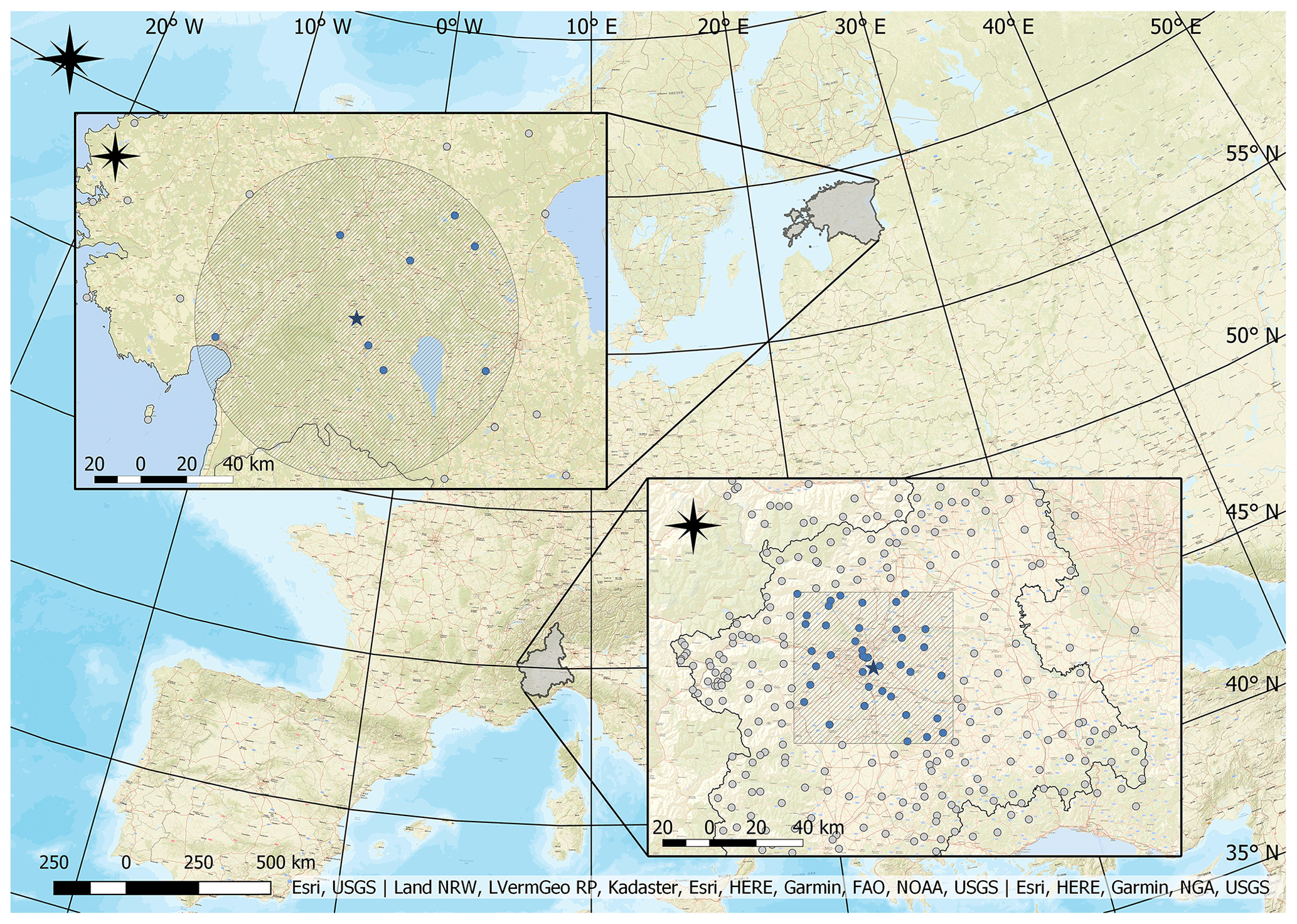
Figure 1Study areas (shaded) located in Estonia (upper left zoomed-in area) and in Piemonte, Italy (lower right zoomed-in area). Grey dots denote gauge locations of both the Estonian and Piemonte region and blue dots gauges inside the study area. Blue stars reveal radar locations.
On the Turin hill, at an altitude of 770 m a.s.l., the operational dual-polarization Doppler C-band weather radar Bric della Croce is located. The radar site is in the central part of the Piemonte region: toward west and north at about 20 km the Alps start, with peaks 2500–3000 m above sea level. The radar performs fully polarimetric volume scans, made up of 11 elevations up to the 170 km range, with 340 m range bin resolution. Bric della Croce observations used in the study ranged from 2012 to 2016, whereas observations from 2012 to 2013 have a 10 min interval and from 2013 to 2016 have a 5 min interval. As can be seen from Fig. 1, a circular area around the radar is used in Estonia, but in Italy a rectangular area is used. The reason for this is that orography in Piemonte is very complex, ranging from flat plains in the Po valley (about 100 m a.s.l.) to the Alps up to more than 4000 m a.s.l. The Bric della Croce weather radar is located on Turin hill, which is about 30 km from the Alps. Therefore, the elegant and simple limitation in range by some kilometres from the radar site does not work. To avoid mountainous areas, where there is partial and total beam blocking and where heavy ground contamination increases, a rectangle area, that extends towards flat grounds, has been preferred.
The maximum distance of the gauges to be included in the comparison was limited to a 70 km radius from the radar location in the case of Estonia and up to 30 km distance in Italy. Thus, in Estonia and Italy rainfall data were from 8 and 42 gauges respectively. By limiting data analysis to the warm season, and constraining the maximum radar range, we were able to ensure that radar data were mainly originating from liquid precipitation (hail can also occur), which is required for more reliable rainfall intensity estimation. The possible occurrence of hail was not removed from the data because of the intention to keep additional data processing minimal and to allow for equal comparison of the various QPE methods. In the case of Italy, the applied range limit is also aimed at eliminating uncertainties due to complex orography, like shielding by the mountains, overshooting, and bright-band contamination.
QPEs, based on horizontal reflectivity, are extensively described by Cremonini and Bechini (2010) and by Cremonini and Tiranti (2018); meanwhile, KDP precipitation estimates are derived according to Wang and Chandrasekar (2009). When KDP was equal to or less than zero, then R(KDP) was set to zero. The area close to the weather radar up to 8 km has been left out due to heavy ground clutter contamination and unreliable estimations of KDP.
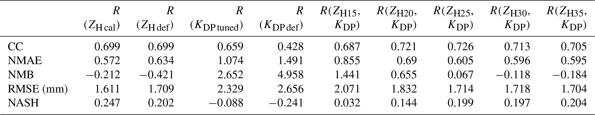
The Sürgavere radar specific differential phase product (KDP) and differential propagation phase product (ØDP) were recalculated from raw ØDP data using the Python ARM Radar Toolkit (Py-ART) (Helmus and Collis, 2016) function phase_proc_lp (Giangrande et al., 2013), with carefully tuned parameter values according to data specifics. With default parameter values, the rays where differential propagation phase folding occurred did not unfold correctly, and thus the function did not produce correct specific differential phase values. To fix the folding issue, function parameters self_const (self-consistency factor) and low_z (the low limit for reflectivity – reflectivity below this value is set to this limit) had to be tuned. The self-consistency factor takes into account the spatial variability of reflectivity and differential reflectivity within a given path. It is used to improve KDP field behaviours to more closely follow the cell patterns found in ZH. The default values for self_const and low_z were 60000.0 and 10.0 respectively, and after testing with various combinations of various values the values 12000.0 and 0.0 were found to produce optimal results and therefore were chosen for final calculations. The values were first chosen after preliminary tests with single scans from multiple years between 2011–2018 and then confirmed after a final test with 1 month of 1 h accumulation data from August 2018. The quality of the results was evaluated by using the verification measures introduced in Sect. 2.1 (Eqs. 1–5). The final test results are shown in Table 1. The product with optimal values for the KDP processing algorithm (R(KDP tuned)) improves all verification measures when compared to the product based on the KDP processing with default parameter values (R(KDP def)). The KDP retrieval process involves filtering that reduces the range resolution of KDP to approximately 1 km. Horizontal reflectivity (ZH) was recalibrated using a method that utilizes the knowledge that ZH, ZDR (differential reflectivity), and KDP are self-consistent with one another and that one can be computed from two of the others. ZDR is not suitable for QPE on C-band radars, but it can be used in this calibration methodology after applying strict restrictions on the data used for this purpose. The calibration was carried out using the self-consistency theory set down in Gorgucci et al. (1992, 1999) and Gourley et al. (2009), where the methodology is described in detail. The method essentially compares the observed differential propagation phase product () to a calculated theoretical differential propagation phase product (ØDPth). The data used for calibration had to be filtered using several restrictions: only data from June to September were allowed; only data from 0.5∘ elevation and 10–70 km range were used; only bins where the horizontal and vertical polarization channel correlation coefficient was over 0.92 were used; any bins where ØDP was greater than 12∘ were removed; whole rays where reflectivity was greater than 50 dBZ were removed; whole rays where ZDR was greater than 3.5 dB were rejected; only rays where was greater than 8∘ and where the consecutive rain path was at least 10 km were used; any scans in which precipitation occurred on top of the radome were removed. As a result, ZH bias values from the range of −2.0 to −5.0 dB were obtained depending on the date. The bias values were used to correct the corresponding observed ZH before to rain rate estimation. The impact of the recalibration was evaluated on 1 month of 1 h accumulation data from August 2018 using the verification measures introduced in Sect. 2.1 (Eqs. 1–5). The verification results are presented in Table 1. The QPE product based on recalibrated reflectivity (R(ZH cal)) shows clearly superior results compared to the non-calibrated reflectivity-based product (R(ZH def)), most notably by decreasing the negative bias.
To convert reflectivity ZH to rainfall rate R (mm/h), the following relation was used:
Specific differential phase KDP was converted to rainfall rate using the expression suggested by Leinonen et al. (2012):
The QPE of R(ZH) can be affected by attenuation on C-band radars, especially in heavy precipitation and at long distances. While this can be corrected using ØDP in our study, it was not applied to the reflectivity data so as to not introduce another possible source of error between the results of Estonia and Italy that could not be easily quantified. The effectiveness of attenuation correction using ØDP is hampered by its temperature, shape, and size distribution dependence, which affect the accompanying error (Vulpiani et al., 2008). The QPE of R(ZH) can also be affected by the effect of the non-uniform vertical profile of reflectivity (VPR). In the current study, the effect of VPR will be limited because only data from the warm season were used, and distance limits to the radar data were set (70 km for Estonia and 30 km for Italy, respectively).
Several studies have shown that R(KDP) provides much more reliable intensity estimates in heavy rainfall (Vulpiani et al., 2012; Wang et al., 2013; Chen and Chandrasekar, 2015). On the other hand, it has been indicated that KDP retrieval itself is less reliable in light precipitation conditions (Giangrande and Ryzhkov, 2008; Ryzhkov et al., 2014). Thus, combining the two methods has the potential to be superior to using each method separately. For example, Vulpiani et al. (2013) used a weighted combination of R(ZH) and R(KDP), where only reflectivity data were used for bins with KDP less than or equal to 0.5∘/km, and KDP was used additionally with increasing weight above that value up to 1∘/km, above which it was solely used. Cifelli et al. (2011) used a simple threshold method where R(KDP) was used when R(ZH) exceeded 50 mm/h intensity. Several authors have successfully added R(ZDR)-based intensity estimation to the combination of S-band weather radars (e.g. Ryzhkov and Zrnic, 1995; Ryzhkov et al., 2005; Chandrasekar and Cifelli, 2012). Due to residual effects such as resonance, noise, and attenuation, R(ZDR) should not be used for C-band radars (Ryzhkov and Zrnic, 2019).
In our study rainfall from a combined threshold approach was used for both weather radars as a third product R(ZH,KDP). In the combined product, R(ZH) was used in areas with ZH less than or equal to 25 dBZ and R(KDP) otherwise if available. The ZH threshold value was selected after testing with various reflectivity levels. The reflectivity threshold was selected after verifying QPE performances at different reflectivity levels from 15 to 35 dBZ in 5 dBZ steps. The evaluation was based on 1 h accumulation rainfall for August 2018 in Estonia, and the verification statistics introduced in Sect. 2.1 (Eqs. 1–5) were applied using the same gauges employed in the latter parts of the study as reference. From Table 1 it can be seen that the best scores are reached using 25 dBZ (QPE product R(ZH25,KDP)). The same evaluation for the R(ZH,KDP) algorithm was carried out for Bric della Croce in Italy with a 1 h accumulation period, and it also confirmed the suitability of the 25 dBZ level. The threshold level is considerably lower than some of the thresholds used in the literature referred to above, but on our datasets it performed the best.
Table 1Verification results of the test dataset of 1 month (August 2018) of the radar-based rainfall 1 h accumulation products of Estonia. ZH is not corrected for attenuation.
The impact of the temporal sampling was analysed using Italian Bric della Croce weather radar second-elevation PPI (plan position indicator) data, which produce a 5 min interval dataset. A degraded dataset of a length of 1 d, 10 October 2020, with a 15 min sampling rate, was created by removing two out of three files. Hourly accumulation was calculated based on both sampling rates, which resulted in a sample size of 253 514. As expected from the comparison of these accumulation pairs, the obtained normalized mean bias was close to zero (0.03), while the correlation coefficient was 0.922, and the normalized mean absolute error was 0.21.
If we compare different skill scores for 1 h QPEs in Estonia and Italy, part of the differences in correlation coefficient and normalized mean absolute error can be explained as being due to different time sampling. Table 2 below summarizes correlation coefficient and normalized mean absolute error values in Estonia and Italy.
Table 2Verification of the 1 h accumulation QPE products of Estonia and Italy and differences without (“Difference”) and with (“Comp. diff”) compensating for the impact of the temporal sampling. CC and NMAE values are obtained from Tables 3 and 4. ZH is not corrected for attenuation.
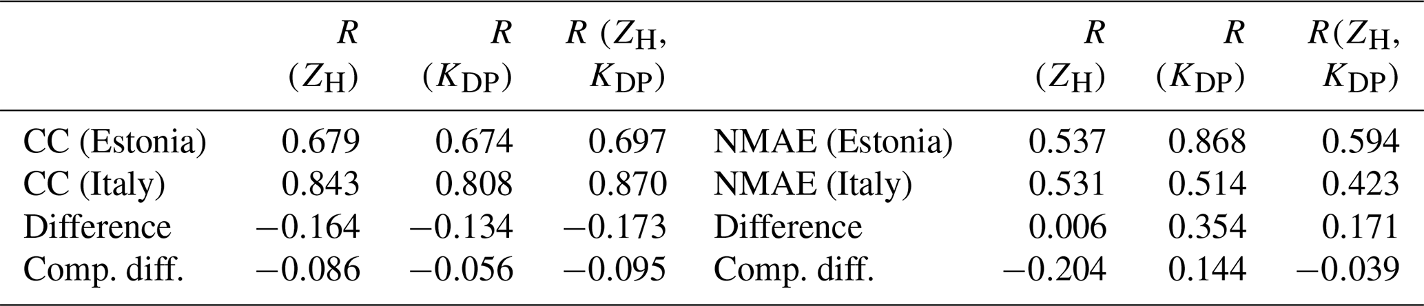
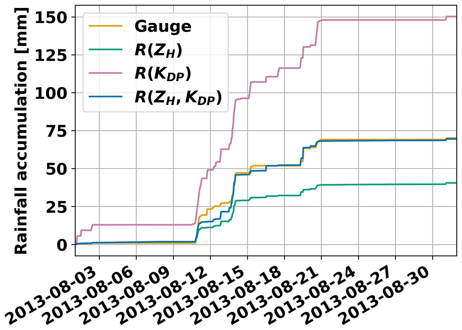
Figure 2The 1-month 1 h rainfall cumulative accumulations for Sürgavere radar data and Jõgeva station gauge data. ZH is not corrected for attenuation.
Compensating the values obtained in Estonia for loss of correlation (0.078) and increased NMAE (0.21) due to 15 min time sampling with values estimated in Italy, it is visible that CC and NMAE are comparable in Estonia and Italy (last row in Table 2). It is worth noting that after the compensation is applied, QPE estimated by R(ZH) shows lower NMAE in Estonia. The difference in NMAE of R(KDP) and R(ZH) QPEs might stem from different precipitation regimes (more intense precipitation in Italy).
3.1 Case comparisons
In this section radar QPE products are compared with single-location gauge measurements of selected short periods from Estonia and Italy. This allows for evaluating the performance of the radar QPE against gauge measurements from a time-series viewpoint.
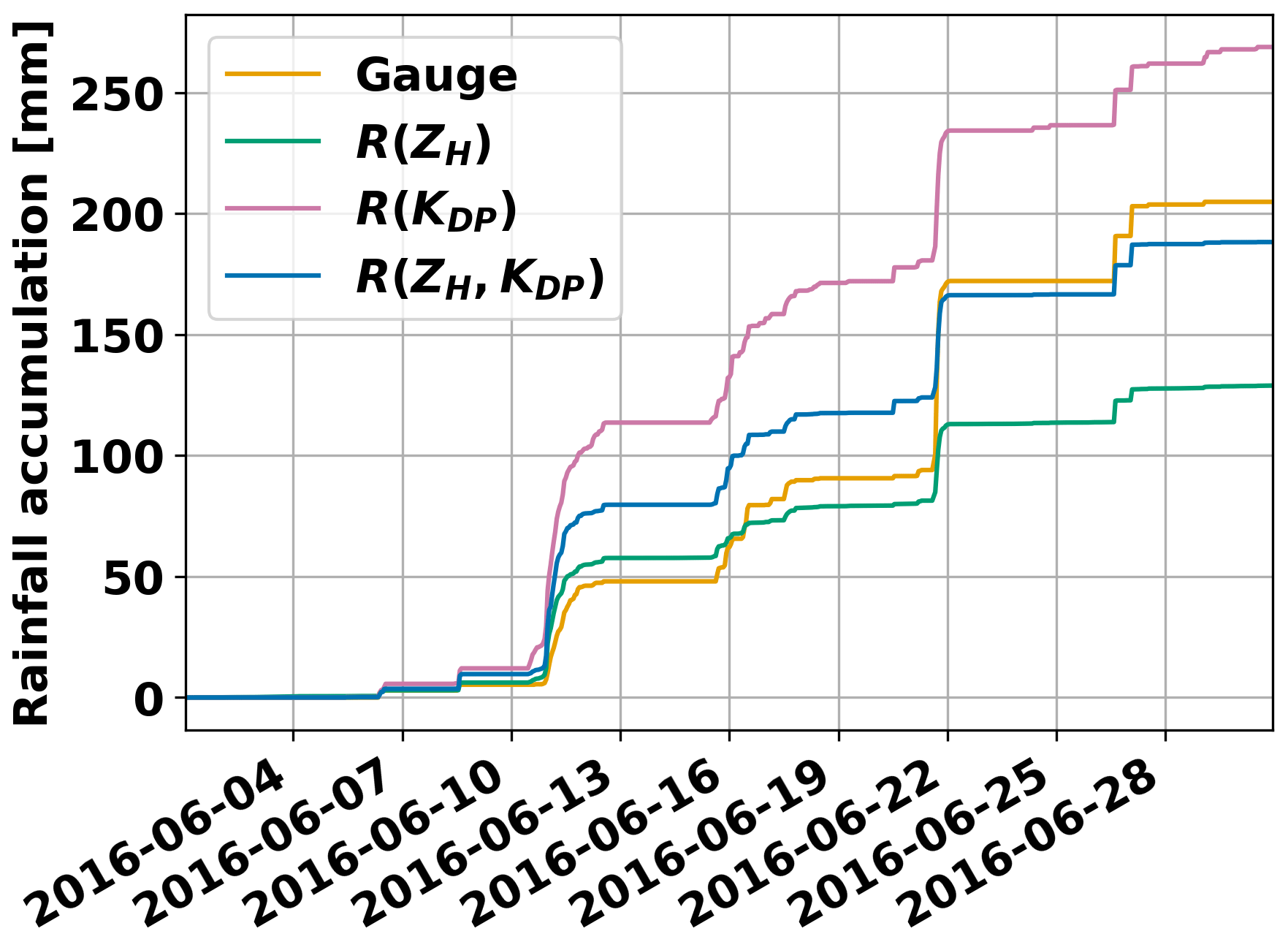
Figure 3The 1-month 1 h rainfall cumulative accumulations for Sürgavere radar data and Tartu-Tõravere station gauge data. ZH is not corrected for attenuation.
Figure 2 shows 1 month of precipitation at the Jõgeva station location (60 km away from the radar site) in Estonia with 1 h temporal resolution. Overall, radar products follow the gauge measurements well, but there are considerable differences among them. Reflectivity-based product R(ZH) is not affected by noise and clutter in clear weather or light rain cases, but on the other hand, it underestimates rainfall amounts particularly in medium- to heavy-precipitation cases. By the end of the month, its sum of 40.5 mm was 19.6 mm less than gauge-measured accumulation (70.1 mm). R(KDP) then again heavily overestimates precipitation amounts, especially during light rain cases. By the end of the month, the accumulated amount of 150.2 mm was more than double the gauge sum. The third product, R(ZH,KDP), showed the best performance of all the three compared, and it correlated well with gauge accumulation time series; the 1-month accumulation of 69.5 mm was just 0.6 mm lower than the rain gauge sum.
Gauge and radar accumulations are not always so well correlated as Fig. 3 demonstrates. In this accumulation period, there are rainfall events which show that gauge values can be both under- and overestimated by radar products. Rainfall around 11 June 2016 is overestimated by all radar QPE products, with the smallest overestimation by R(ZH) and greatest by R(KDP), which overestimated the gauge by more than 2 times in this event. In the following days until 21 June 2016, light to medium precipitation was recorded by the gauge, and during this time R(KDP) mostly overestimated the gauge accumulations, while R(ZH) underestimated rainfall. On the 21 June 2016, a convective rainfall event occurred during which 51 mm of rainfall was measured in 2 h with a gauge. All radar QPE products underestimated the rainfall amount during this event. By the end of the month-long accumulation period, R(ZH,KDP) was closest to the gauge value (underestimation by 16.6 mm), while R(ZH) underestimated even more, and R(KDP) again overestimated gauge measurements.
Figure 4 illustrates a case from Italy, a comparison of a gauge located within 30 km distance from the radar to Bric della Croce radar precipitation estimation products. At the end of the 34 h period, the specific differential-phase-based product R(KDP) has the smallest error compared to gauge as it overestimates the gauge measurement of 40.6 mm by 2.0 mm. On the other hand, in light rain R(KDP) overestimated significantly – in the first 13 h when a gauge measured 3.4 mm of accumulated rainfall, it had already estimated 12.2 mm. R(ZH) underestimated, even in light rain, and in heavy rain, the difference compared to gauge measurement increased further. At the end of the period, the underestimation was nearly 3-fold (15.6 mm compared to gauge accumulation of 40.6 mm). The R(ZH,KDP) product showed good correlation with gauge measurement in light precipitation as it was mostly based on reflectivity data, but in the case of more intense precipitation, it still underestimated compared to gauge data. At the end of the period, the accumulated value for R(ZH,KDP) was 26.7 mm.

Figure 4The 1 h rainfall cumulative accumulations from Verolengo gauge, located 29 km from the radar, and co-located Bric della Croce radar QPE. ZH is not corrected for attenuation.
In all selected cases the general behaviour of QPEs is similar. Weather radar estimations, even when sampled by 15 min interval observations, follow gauge measurements with good agreement, although the second case from Estonia illustrated well that a longer scan interval increases the scatter and particularly with small-scale convective precipitation, for which a minimal sampling interval is the most beneficial. From Italy, the example case was much shorter, but the precipitation intensity was higher. In both cases, R(KDP) generally overestimates precipitation amounts, especially in light rain cases. In Italy, the R(KDP) overestimation is smaller. One of the causes of this behaviour might be more intense precipitation in Italy for which KDP measurement was more accurate. More intense rainfall on the other hand caused greater underestimation of R(ZH)-based precipitation accumulation from gauge values compared to Estonia. Another cause of differences between the two countries might be differences in the drop size distribution climatologies. Rainfall retrieval relations also cause errors, and to keep the comparison as uniform as possible, we decided to use the same relations for both Italy and Estonia. These example cases demonstrated that radar can be used for 1 h accumulations, but systematic errors cannot be excluded. These cases also presented the shortcomings of studies based only on a few cases. The performance of a QPE method depends heavily on a chosen case, and it might perform differently on a long-term analysis. Errors and uncertainties will be calculated and how QPEs compare to gauge measurements on a longer scale will be looked at in the next sections.
3.2 Comparison of 1 h accumulations
The quality of the rainfall estimates is compared at various accumulation intervals. Comparing different intervals can also be useful to point out representativeness issues caused by low radar scan rates. The investigated period covers the years 2011–2018 in Estonia and 2012–2016 in Italy.
First, in this section hourly accumulations are analysed. Hourly accumulations are especially important for small basins and in extreme precipitation climatology analysis. Hourly rainfall maxima can provide valuable data for flash flood nowcasting and other hydrological applications.
Table 3Verification of the radar-based rainfall 1 h accumulation products of Estonia. ZH is not corrected for attenuation.
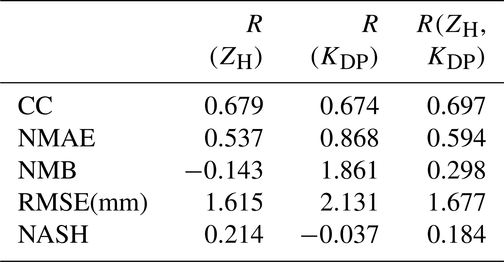
Table 4Verification of the radar-based rainfall 1 h accumulation products of Italy. ZH is not corrected for attenuation.
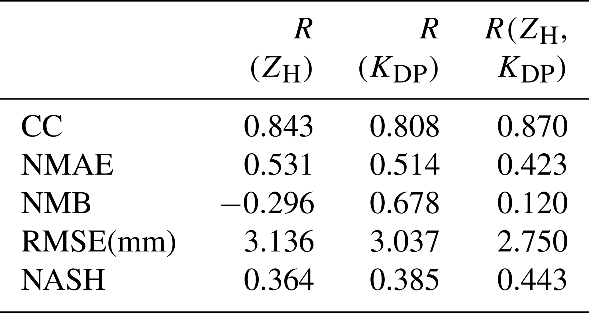
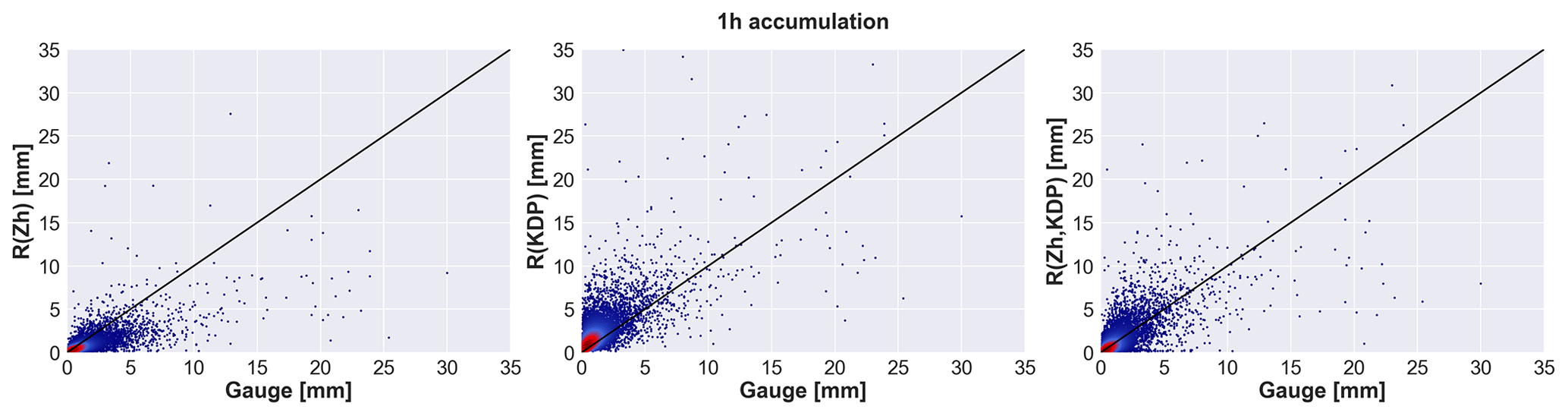
Figure 5Scatter plots of radar-based rainfall estimates against rain gauge observations for 1 h accumulation intervals in Estonia 2011–2018. The corresponding verification measures are presented in Table 3. The number of radar–gauge data pairs with eight gauges and accumulations >0.1 mm is 7019. ZH is not corrected for attenuation.
Table 3 presents the verification results for the hourly accumulation interval in Estonia. Figure 5 shows the corresponding scatter plots. As can be seen, the R(ZH) estimation generally underestimates rainfall, especially heavy events, while it has the best error verification values (Nash–Sutcliffe efficiency 0.214, NMAE 0.537, NMB −0.143, and RMSE 1.615 mm). R(KDP) on the other hand overestimates accumulations for low-intensity events as could be presumed. R(ZH,KDP) shows considerable improvement by combining strong aspects of the two methods. It has the highest correlation coefficient (0.697) of all the products.
Nevertheless, it can be seen from the scatter plots that there is a lot of scatter in the hourly radar accumulations with all products. Mostly, it can be linked to the low spatial representativeness of the point measurements of rain gauges. This effect is more pronounced on a short timescale, and it originates from a scarce gauge network and insufficient radar scan rate. Small-scale effects like wind drift might also be more influential on a shorter accumulation period (Lauri et al., 2012). The reason why R(ZH) might have the best performances when NMAE and RMSE are considered is that there are not very many heavy rainfall cases in Estonia, and this tends to favour R(ZH) in the verification comparisons.
From Italian hourly accumulation scatter plots in Fig. 6, it can be seen that the overall behaviour of the radar products is similar to Estonia, although from Fig. 6 it can be noticed that of the four highest 1 h accumulations measured by the gauge, three of them have significantly higher radar estimates for R(ZH,KDP) than either R(ZH) or R(KDP). This could be explained by precipitation that was very variable in intensity and also in spatial coverage in these three cases, which in turn caused unsteady behaviour of the precipitation estimates. ZH underestimates high intensities, but with low intensities, KDP becomes noisy, and the rainfall intensity estimation is not feasible. Finally, to reduce KDP uncertainties, range averaging is mandatory, leading to underestimation in the case of very localized showers. By blending both R(ZH) and R(KDP), a better rainfall estimation is expected. Table 4 presents the corresponding verification results. R(ZH) underestimates rainfall, particularly for intense precipitation events. R(KDP) generally overestimates hourly accumulations, especially at low-intensity cases: as stated by Wang et al. (2013), R(KDP) generates noisier estimations at low rain rates. R(ZH,KDP) outperforms both other products in Italy, which is confirmed by verification metrics as it overcomes the shortcomings of the other estimations.
Less random scatter is visible in Italian hourly data due to the more frequent scan strategy. R(ZH) underestimated accumulations more than in Estonia as expected because in Italy intense rainfall is more frequent – it has a larger RMSE and an even more negative NMB. Probably for the same reason, R(KDP) is more accurate in Italy than in Estonia as it has a smaller NMAE and NMB while having a larger RMSE due to higher rainfall intensities recorded in Italy.
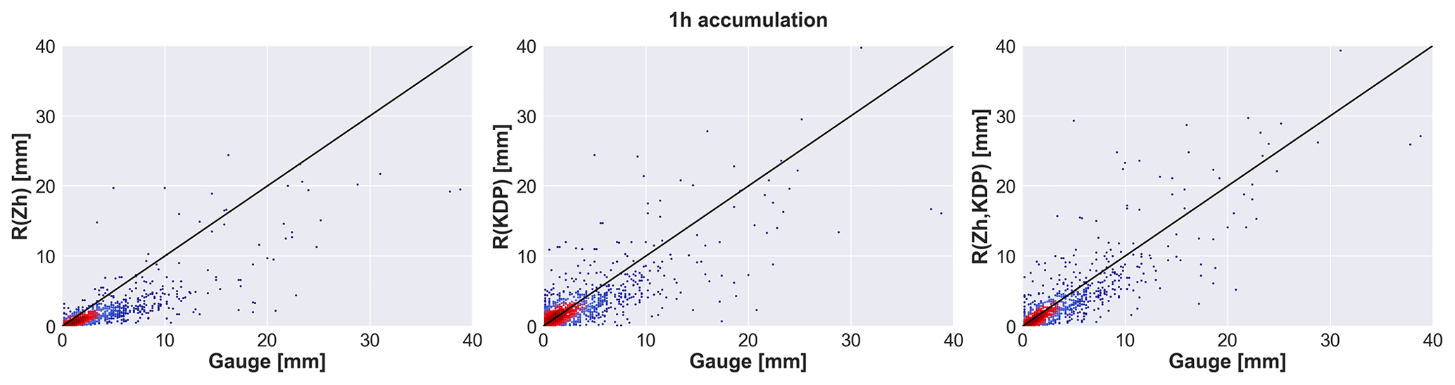
Figure 6The 1 h accumulations for Italy, 2012–2016. The corresponding verification measures are presented in Table 4. The number of radar–gauge data pairs with 42 gauges and accumulations >0.1 mm is 1233. ZH is not corrected for attenuation.
Table 5Verification of the radar-based rainfall 24 h accumulation products of Estonia. ZH is not corrected for attenuation.
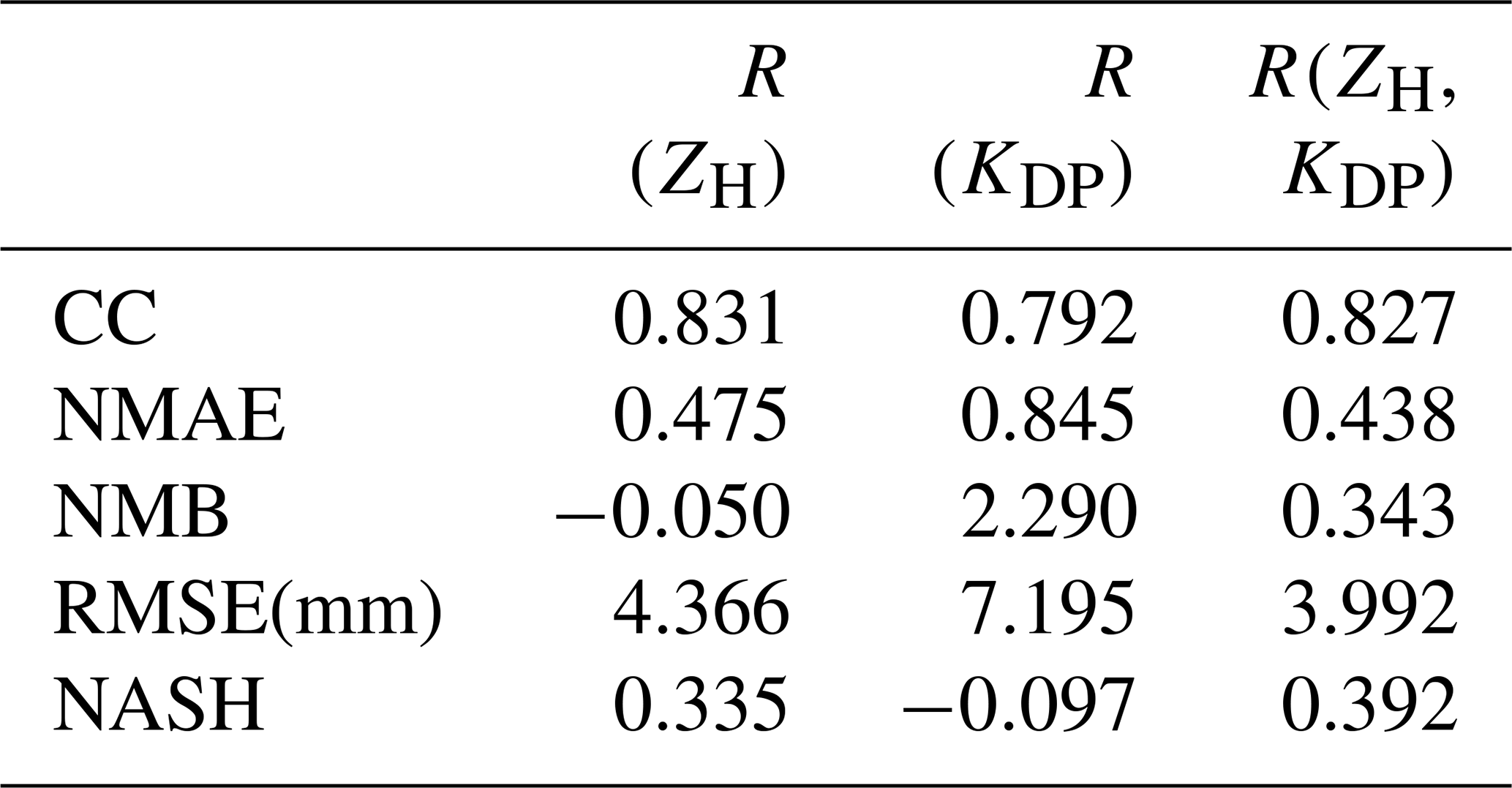
Table 6Verification of the radar-based rainfall 24 h accumulation products of Italy. ZH is not corrected for attenuation.
3.3 Comparison of 24 h accumulations
Table 5 shows the verification results for the daily accumulation interval in Estonia, while Fig. 7 presents the corresponding scatter plots. As expected, much less scatter can be seen than on the daily level, but overall, the results are consistent with the hourly interval verification outcomes. Using longer accumulation intervals leads to less severe errors as the longer period compensates for both underestimates and overestimates. The reflectivity-based product, R(ZH), still underestimated rain depths, while the negative bias is considerably smaller than in hourly interval data. By looking at the definition of NMB in Eq. (3), it can be seen that in the case that the same underlying samples are used, NMB should be equal on all accumulation lengths. In our study, the underlying samples were different as the 0.1 mm threshold was applied after the accumulation as the last step before calculating the verification metrics. This emphasizes the importance of low-intensity precipitation for total accumulations. R(KDP) is the least accurate of the three products, also on a daily accumulation level, with the lowest correlation and highest error scores. The combined product, R(ZH,KDP), removes the negative bias of R(ZH) and shows better correlation and substantial improvement in terms of both the systematic error and the overall error compared to R(KDP). R(ZH,KDP) has the smallest NMAE of 0.438, a RMSE of 3.992 mm, and the highest Nash–Sutcliffe efficiency, equal to 0.392. Overall there is noticeably less scatter in the daily radar accumulations compared to the 1 h interval.
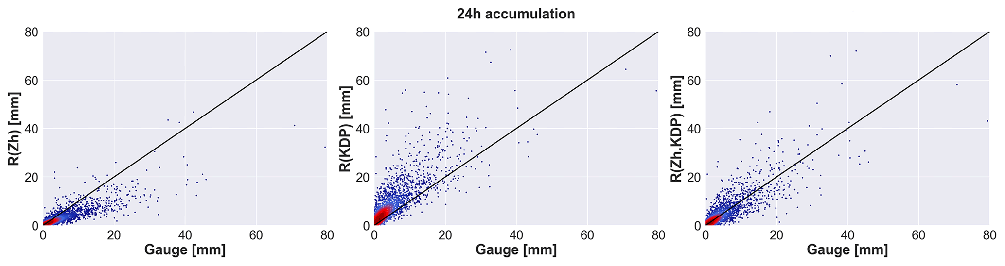
Figure 7The 24 h accumulations for Estonia, 2011–2018. The corresponding verification measures are presented in Table 5. The number of radar–gauge data pairs with eight gauges and accumulations >0.1 mm is 2148. ZH is not corrected for attenuation.
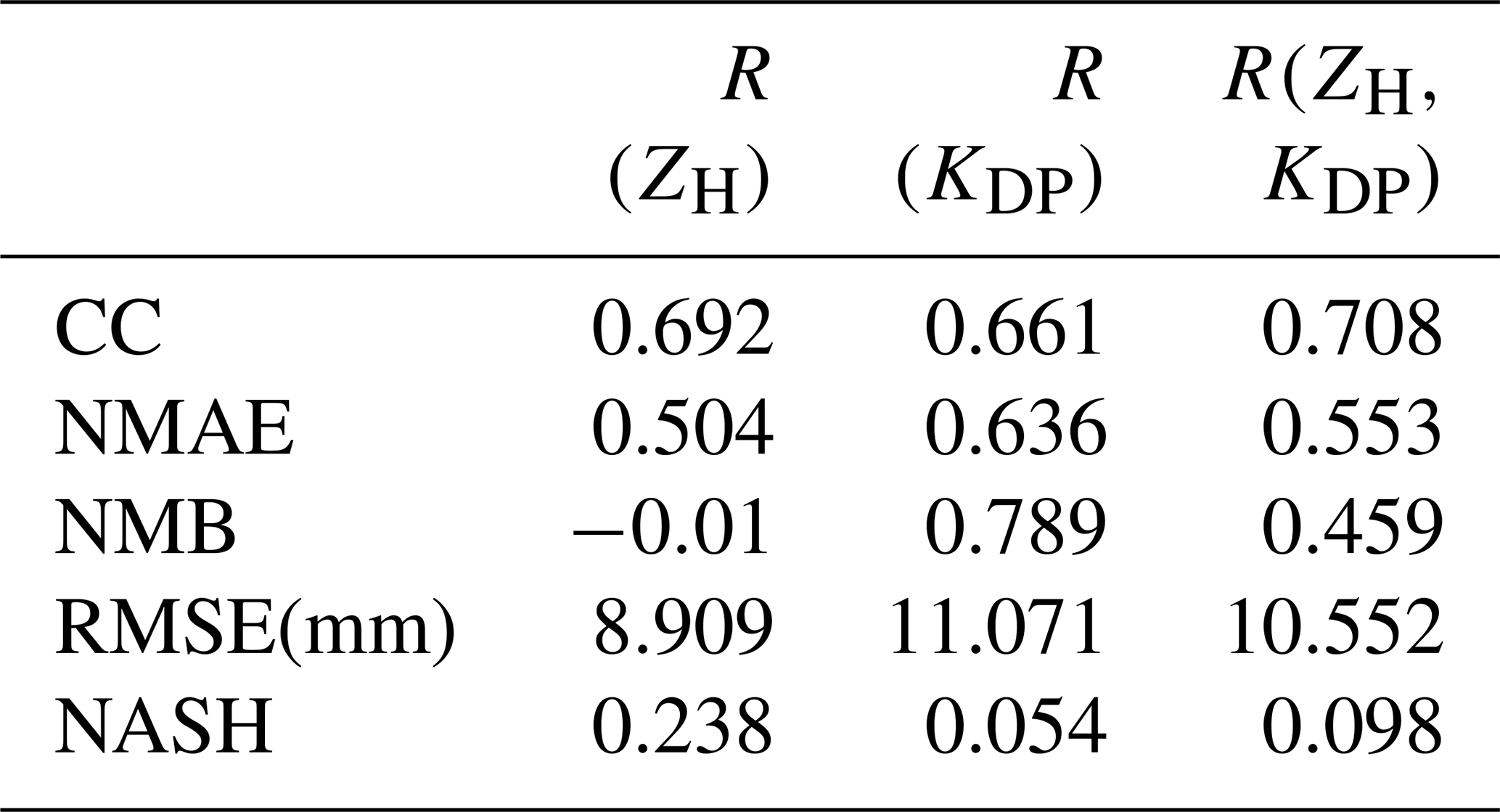
Table 6 shows the verification results for the daily accumulation interval in Italy, while Fig. 8 presents the corresponding scatter plots. R(ZH) slightly underestimated accumulations compared to gauge results, and surprisingly it outperforms other competing products in all metrics except Pearson's correlation coefficient. R(KDP) again overestimated accumulations the most and has the lowest correlation with gauge data. R(ZH,KDP) notably improves the R(KDP) in all verification metrics but does not exceed R(ZH), except for the correlation coefficient, which is the highest of all three products with an r of 0.708. In Italy, the decrease in scatter of radar accumulations cannot be observed compared to the 1 h level. In Fig. 7 two regimes can be observed, and we assume that VPR correction leads to these regimes. Bric della Croce weather radar is located on a top of a hill at 770 m a.s.l., and during the winter season, a vertical profile reflectivity correction (VPR) is applied (Koistinen, 1991). This correction is manually switched on at the beginning of the cold season, and it is switched off at the end. In the case of convective precipitation, this correction may lead to rainfall overestimation. On the other hand, stratiform cold precipitation is heavily underestimated when VPR correction is switched off.
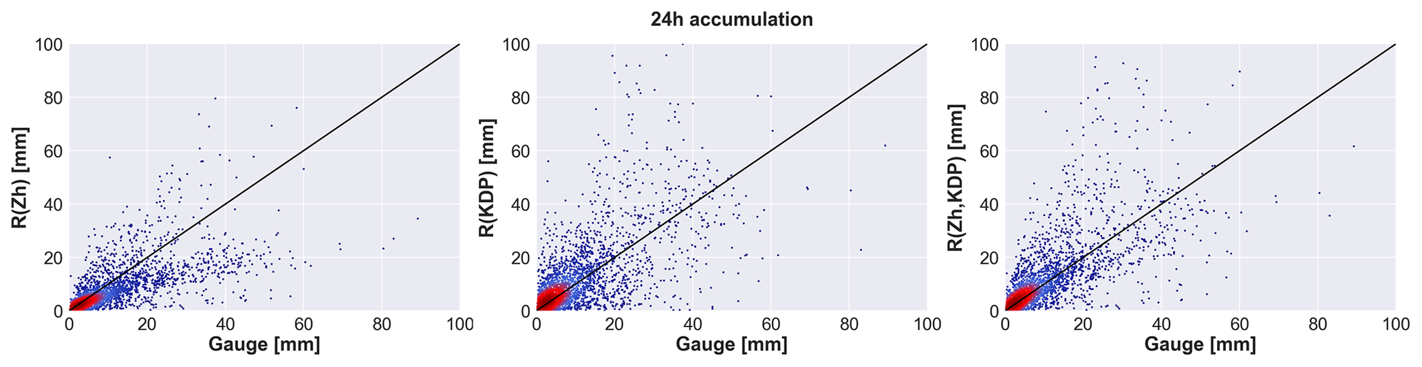
Figure 8The 24 h accumulations for Italy, 2012–2016. The corresponding verification measures are presented in Table 6. The number of radar–gauge data pairs with 42 gauges and accumulations >0.1 mm is 3010. ZH is not corrected for attenuation.
3.4 Comparison of monthly accumulations
Table 7 shows the verification results for the monthly accumulation interval in Estonia, while Fig. 9 presents the corresponding scatter plots. Compared to shorter timescales, overall on a monthly scale the correlation of all the products with gauge accumulations is higher. R(ZH) underestimated accumulations, with a larger mean bias (−0.284) than on a daily level but with a smaller normalized mean absolute error (0.360). R(KDP) showed less scatter than on shorter timescales like other products while it still heavily overestimated accumulations (NMB equal to 1.042 with a RMSE equal to 62.466 mm). On the monthly accumulation level, R(ZH,KDP) outperforms the two other products to a great extent. It is well correlated to gauge values with small scatter as it performs very well, both in low- and high-accumulation cases. The correlation coefficient is nearly identical to R(ZH), but it removes the systematic underestimation of R(ZH) and overestimation of R(KDP) and exceeds them in all other verification metrics.
Table 7Verification of the radar-based rainfall monthly accumulation products of Estonia. ZH is not corrected for attenuation.
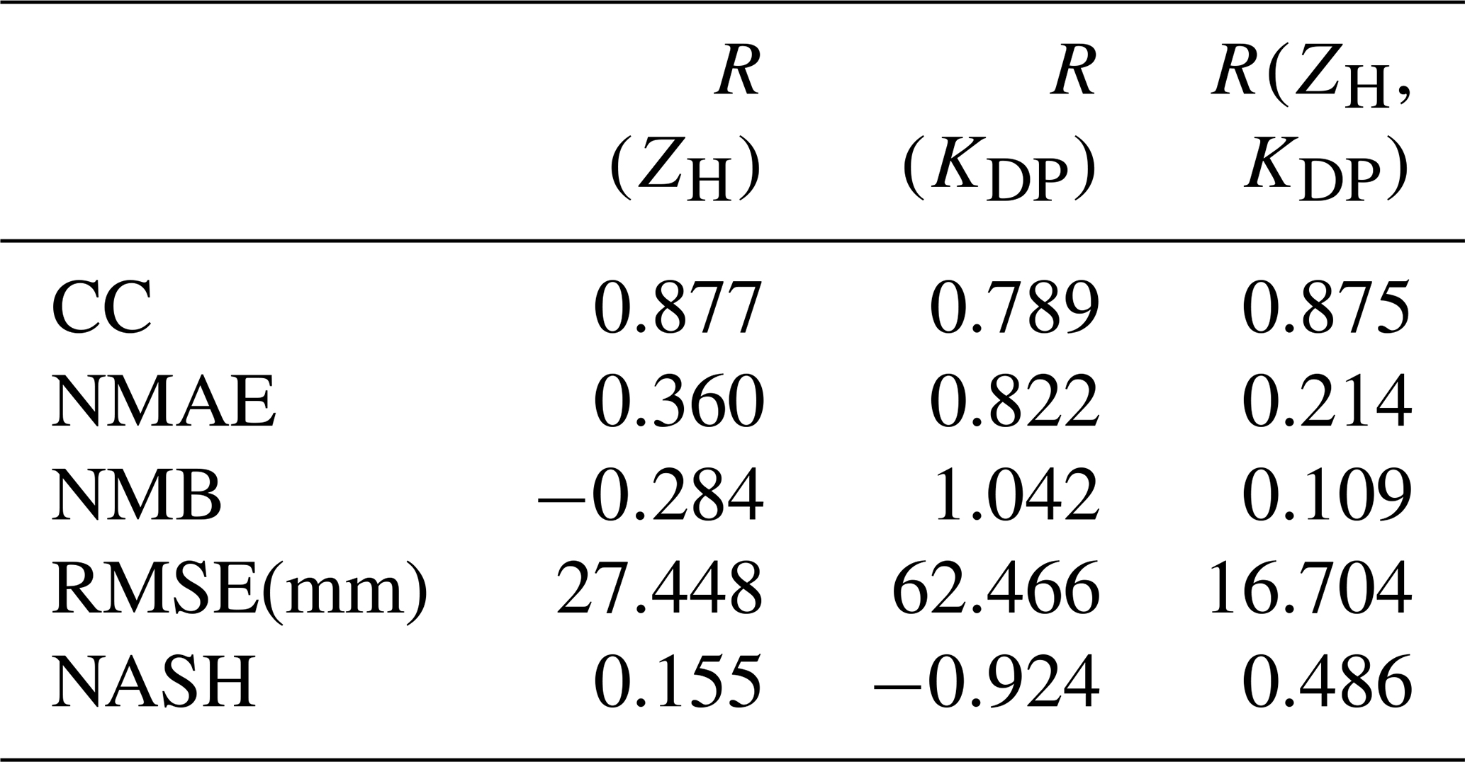
Table 8Verification of the radar-based rainfall monthly accumulation products of Italy. ZH is not corrected for attenuation.
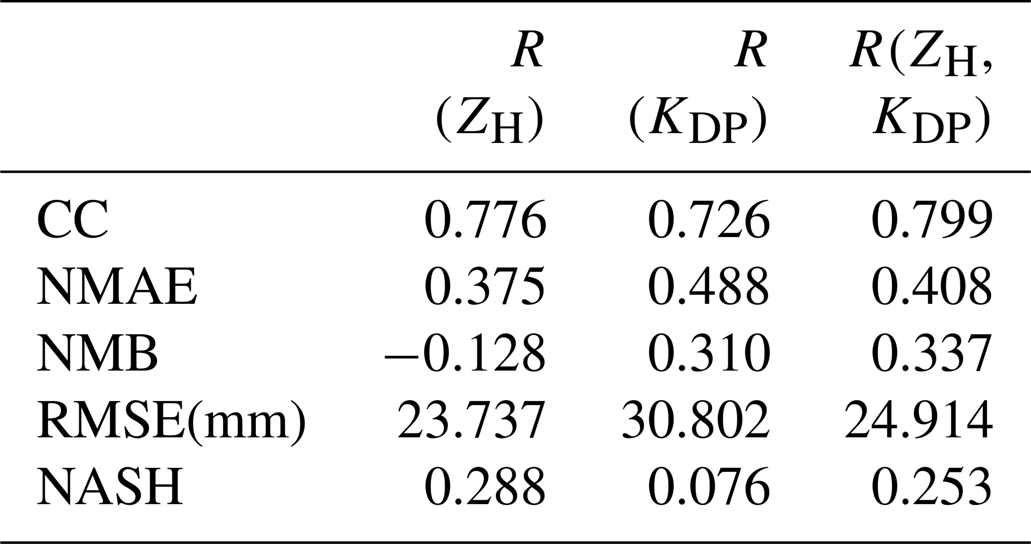
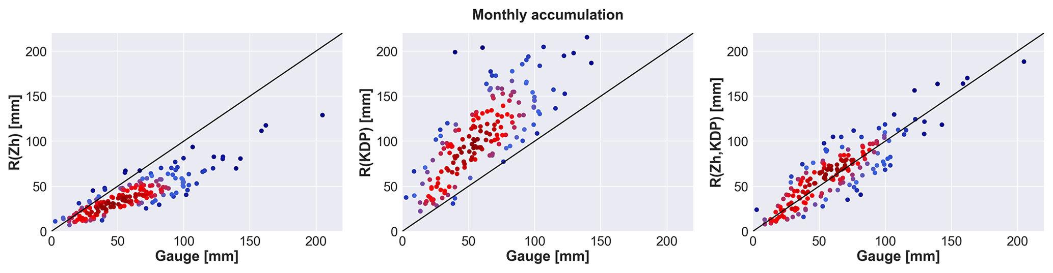
Figure 9Monthly accumulations for Estonia, 2011–2018. The corresponding verification measures are presented in Table 7. The number of radar–gauge data pairs with eight gauges is 179. ZH is not corrected for attenuation.
Table 8 shows the verification results for the monthly accumulation interval in Italy, while Fig. 10 presents the corresponding scatter plots. Scatter plots reveal similar characteristics to the daily level accumulations of the products. R(ZH) underestimated rainfall, also on a monthly scale, and R(KDP) overestimated rainfall. R(ZH, KDP) still overestimated rainfall but with a decreased RMSE compared to the R(KDP) product. It also exhibits the highest correlation coefficient of the three. According to the verification results, most of the metrics indicate better performance of the radar products on a monthly scale compared to daily intervals. The correlation coefficient is higher and the NMAE is lower for all the products when the two timescales are compared.
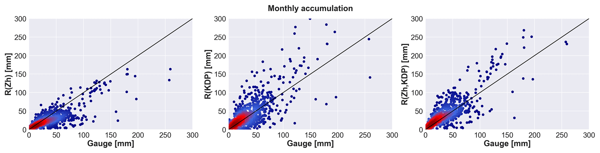
Figure 10Monthly accumulations for Italy, 2012–2016. The corresponding verification measures are presented in Table 8. The number of radar–gauge data pairs with 42 gauges is 675. ZH is not corrected for attenuation.
In the present study polarimetric rainfall retrieval methods for the fully operational C-band radars in Sürgavere, Estonia, and Bric della Croce, Italy, have been analysed. The study focuses on the warm period of the year, and a long period of multi-year data is used. From Estonia 5 years of data from 2011 to 2018 has been included; from Italy, the data interval ranges from 2012 to 2016. Reflectivity data were calibrated following a self-consistency theory, and measured horizontal reflectivity (ZH) was corrected accordingly. To calculate rainfall from polarimetric variables, the differential propagation phase product (ØDP) was reconstructed, and based on that the specific differential phase product (KDP) was retrieved. To achieve this the transparently implemented algorithm phase_proc_lp (Giangrande et al., 2013) in the open-source toolkit Py-ART was used for Estonian data. For Italian data, KDP precipitation estimates were obtained following the theory set down in Wang et al. (2009).
Three radar rainfall estimation products were computed: a horizontal reflectivity-based product R(ZH), a specific differential-phase-based product R(KDP), and a combined product based on the previous two R(ZH,KDP). Rain gauge network data of Italy and Estonia were used as ground truth. The 1 h, 24 h, and monthly accumulations were derived from the radar products and gauge data.
Time-series comparison revealed that even with a 15 min scan interval, radar is suitable for QPE, at least with more widespread precipitation like stratiform rain. Still, on the shortest accumulation period of 1 h, the scarcer radar data from Estonia had more scatter than data from Italy, where the scan interval was 10 min on older data and 5 min since 2013. As an overall trend, the longer the accumulation period, the less scattering that was visible. The case comparisons also revealed the shortcomings of analysis based only on selected short periods. The performance of the QPE methods then depends on the representativeness of the chosen cases, and results can easily be skewed. Using a dataset with a length of at least several years without preselection provides more robust results and allows for evaluating the operational usability of the methods.
When the three products are compared to each other based on the full length of 5 years of data, in the case of Estonia, the R(ZH,KDP) was superior to R(ZH) and R(KDP) in all accumulation periods. Especially on the monthly accumulation scale, it performed distinctly better as it had a RMSE 39% lower than the nearest competitor, the R(ZH) product, and even 73% lower than R(KDP). In Italy, the R(ZH,KDP) product exceeded the two others clearly on an hourly level. On 24 h and monthly accumulation scale, it had the highest correlation with gauge measurements, but the error verification measures were slightly higher than those of the R(ZH). Nevertheless, it outperformed R(KDP) on all timescales.
Overall the results show that the combined product R(ZH,KDP) performs better in almost all of the verification measures in both countries compared to R(ZH) and R(KDP) as it successfully uses the benefits of each other product and eliminates the weaknesses. R(ZH) was good at low precipitation intensities, but in general, it underestimated precipitation. It had an average NMB of −0.159 for all accumulation lengths in Estonia and −0.145 in Italy. R(KDP) performed well at higher intensities but in general overestimated precipitation. It had an average NMB of 1.731 for all the accumulation lengths in Estonia and 0.592 in Italy, while the combined product R(ZH,KDP) slightly overestimated precipitation, with an average NMB of 0.250 for all the accumulation lengths in Estonia and 0.305 in Italy. In both countries the R(ZH,KDP) product also had the highest average CC over all the accumulation lengths, with CC of 0.800 in Estonia and 0.792 in Italy. Generally, the CC was higher the longer the accumulation period was, with the highest CC in monthly accumulations (R(ZH,KDP) CC of 0.875 in Estonia and 0.799 in Italy).
In Estonia, the overestimation of R(KDP) was noticeably higher than in Italy. We hypothesize that this is mostly due to different climatological regimes between Italy and Estonia as high-intensity rainfalls occur more frequently in Italy, although one has to keep in mind that the radars were from different manufacturers and thus also the KDP retrieval algorithms used were different, which might be the cause of some discrepancy. Another source of error might originate from the implemented ZH–R and KDP–R relations, which might not perform equally in different climates. Overall the results of the study showed that dual-polarimetric radar QPE and especially the combined product R(ZH,KDP) show good potential to be used on long-term datasets if certain limitations are considered.
Synoptic patterns could be used as an additional source for classifying the radar accumulations. This would enable the performance of each radar product to be verified for stratiform and convective events. Moreover, it could be used to investigate if frequent scans play a bigger role in convective events than stratiform events as could be hypothesized and to quantify the effect.
For future studies, it would also be useful to calculate probabilities and return periods of extreme rainfall for weather-radar-based rainfall climatology.
The code used to conduct all analyses in this paper is available by contacting the authors. Gauge and radar data used in this study are available by contacting the authors.
TV, RC, PP, and DM directly contributed to the conception and design of the work. TV and RC collected and processed the various datasets and wrote the original draft with input from PP and DM. All authors reviewed and edited the final draft.
The authors declare that they have no conflict of interest.
The authors are grateful to the Meteorological Observation Department of the Estonian Environment Agency for providing rain gauge datasets. The authors would also like to thank editor Laurent Pfister, reviewer Hidde Leijnse, and two anonymous reviewers for their constructive comments that helped to significantly improve the manuscript.
This research has been supported by the Estonian Ministry of Education and Research (grant no. IUT20-11), the Estonian Research Council (grant no. PSG202), and the European Regional Development Fund within the National Programme for Addressing Socio-Economic Challenges through R&D (grant no. RITA1/02-52-07).
This paper was edited by Laurent Pfister and reviewed by Hidde Leijnse and two anonymous referees.
Alber, R., Jaagus, J., and Oja, P.: Diurnal cycle of precipitation in Estonia, Est. J. Earth Sci., 64, 305–313, https://doi.org/10.3176/earth.2015.36, 2015.
Bringi, V. N., Rico-Ramirez, M. A., and Thurai, M.: Rainfall estimation with an operational polarimetric C-band radar in the United Kingdom: comparison with a gauge network and error analysis, J. Hydrometeorol., 12, 935–954, https://doi.org/10.1175/JHM-D-10-05013.1, 2011.
Cao, Q., Knight, M., and Qi, Y.: Dual-pol radar measurements of Hurricane Irma and comparison of radar QPE to rain gauge data, in: Proceedings of the 2018 IEEE Radar Conference, Oklahoma City, OK, USA, 23–27 April 2018, 0496–0501, https://doi.org/10.1109/RADAR.2018.8378609, 2018.
Chandrasekar, V. and Cifelli, R.: Concepts and principles of rainfall estimation from radar: Multi sensor environment and data fusion, Indian J. Radio Space, 41, 389–402, 2012.
Chandrasekar, V., Keränen, R., Lim, S., and Moisseev, D.: Recent advances in classification of observations from dual polarization weather radars, Atmos. Res., 119, 97–111, https://doi.org/10.1016/j.atmosres.2011.08.014, 2013.
Chang, W. Y., Vivekanandan, J., Ikeda, K., and Lin, P. L.: Quantitative precipitation estimation of the epic 2013 Colorado flood event: Polarization radar-based variational scheme, J. Appl. Meteorol. Climatol., 55, 1477–1495, https://doi.org/10.1175/JAMC-D-15-0222.1, 2016.
Chen, H. and Chandrasekar, V.: The quantitative precipitation estimation system for Dallas–Fort Worth (DFW) urban remote sensing network, J. Hydrol., 531, 259–271, https://doi.org/10.1016/j.jhydrol.2015.05.040, 2015.
Cifelli, R., Chandrasekar, V., Lim, S., Kennedy, P. C., Wang, Y., and Rutledge, S. A.: A new dual-polarization radar rainfall algorithm: Application in Colorado precipitation events, J. Atmos. Ocean. Tech., 28, 352–364, https://doi.org/10.1175/2010JTECHA1488.1, 2011.
Cornes, R. C., van der Schrier, G., van den Besselaar, E. J., and Jones, P. D.: An Ensemble Version of the E-OBS Temperature and Precipitation Data Sets, J. Geophys. Res.-Atmos., 123, 9391–9409, https://doi.org/10.1029/2017JD028200, 2018.
Cremonini, R. and Bechini, R.: Heavy rainfall monitoring by polarimetric C-band weather radars, Water-Sui., 2, 838–848, https://doi.org/10.3390/w2040838, 2010.
Cremonini, R. and Tiranti, D.: The Weather Radar Observations Applied to Shallow Landslides Prediction: A Case Study From North-Western Italy, Front. Earth Sci., 6, 134, https://doi.org/10.3389/feart.2018.00134, 2018.
Crisologo, I., Vulpiani, G., Abon, C. C., David, C. P. C., Bronstert, A., and Heistermann, M.: Polarimetric rainfall retrieval from a C-Band weather radar in a tropical environment (The Philippines), Asia-Pac. J. Atmos. Sci., 50, 595–607, https://doi.org/10.1007/s13143-014-0049-y, 2014.
Devoli, G., Tiranti, D., Cremonini, R., Sund, M., and Boje, S.: Comparison of landslide forecasting services in Piedmont (Italy) and Norway, illustrated by events in late spring 2013, Nat. Hazards Earth Syst. Sci., 18, 1351–1372, https://doi.org/10.5194/nhess-18-1351-2018, 2018.
Giangrande, S. E. and Ryzhkov, A. V.: Estimation of rainfall based on the results of polarimetric echo classification, J. Appl. Meteorol. Climatol., 47, 2445–2462, https://doi.org/10.1175/2008JAMC1753.1, 2008.
Giangrande, S. E., McGraw, R., and Lei, L.: An application of linear programming to polarimetric radar differential phase processing, J. Atmos. Ocean. Tech., 30, 1716–1729, https://doi.org/10.1175/JTECH-D-12-00147.1, 2013.
Gorgucci, E., Scarchilli, G., and Chandrasekar, V.: Calibration of radars using polarimetric techniques, IEEE T. Geosci. Remote, 30, 853–858, https://doi.org/10.1109/36.175319, 1992.
Gorgucci, E., Scarchilli, G., and Chandrasekar, V.: A procedure to calibrate multiparameter weather radar using properties of the rain medium, IEEE T. Geosci. Remote, 37, 269–276, https://doi.org/10.1109/36.739161, 1999.
Goudenhoofdt, E. and Delobbe, L.: Generation and verification of rainfall estimates from 10-yr volumetric weather radar measurements, J. Hydrometeorol., 17, 1223–1242, https://doi.org/10.1175/JHM-D-15-0166.1, 2016.
Gourley, J. J., Illingworth, A. J., and Tabary, P.: Absolute calibration of radar reflectivity using redundancy of the polarization observations and implied constraints on drop shapes, J. Atmos. Ocean. Tech., 26, 689–703, https://doi.org/10.1175/2008JTECHA1152.1, 2009.
Gregorč, G., Macpherson, B., Rossa, A., and Haase, G.: Assimilation of radar precipitation data in NWP Models–a review, Phys. Chem. Earth Pt. B, 25, 1233–1235, https://doi.org/10.1016/S1464-1909(00)00185-4, 2000.
Helmus, J. J. and Collis, S. M.: The Python ARM Radar Toolkit (Py-ART), a Library for Working with Weather Radar Data in the Python Programming Language, J. Open Res. Softw., 4, e25, https://doi.org/10.5334/jors.119, 2016.
Koistinen, J.: Operational correction of radar rainfall errors due to the vertical reflectivity profile, Proceedings of the 25th Radar Meteorology Conference, American Meteorological Society, Paris, France, 91–96, 1991.
Krajewski, W. F., Villarini, G., and Smith, J. A.: Radar-Rainfall Uncertainties: Where are We after Thirty Years of Effort?, B. Am. Meteorol. Soc., 91, 87–94, https://doi.org/10.1175/2009BAMS2747.1, 2010.
Lauri, T., Koistinen, J., and Moisseev, D.: Advection-Based Adjustment of Radar Measurements, Mon. Weather Rev., 140, 1014–1022, https://doi.org/10.1175/MWR-D-11-00045.1, 2012.
Leinonen, J., Moisseev, D., Leskinen, M., and Petersen, W. A.: A climatology of disdrometer measurements of rainfall in Finland over five years with implications for global radar observations, J. Appl. Meteorol. Climatol., 51, 392–404, https://doi.org/10.1175/JAMC-D-11-056.1, 2012.
Macpherson, B., Lindskog, M., Ducrocq, V., Nuret, M., Gregoric, G., Rossa, A., Haase, G., Holleman, I., and Alberoni, P. P.: Assimilation of Radar Data in Numerical Weather Prediction (NWP) Models, in: Weather Radar – Principles and Advanced Applications, Springer, Berlin, Germany, https://doi.org/10.1007/978-3-662-05202-0_9, 2004.
Montopoli, M., Roberto, N., Adirosi, E., Gorgucci, E., and Baldini, L.: Investigation of Weather Radar Quantitative Precipitation Estimation Methodologies in Complex Orography, Atmosphere-Basel, 8, 34, https://doi.org/10.3390/atmos8020034, 2017.
Nash, J. E. and Sutcliffe, J. V.: River flow forecasting through conceptual models part I: A discussion of principles, J. Hydrol., 10, 282–290, https://doi.org/10.1016/0022-1694(70)90255-6, 1970.
Overeem, A., Holleman, I., and Buishand, A.: Derivation of a 10 year radar-based climatology of rainfall, J. Appl. Meteorol. Climatol., 48, 1448–1463, https://doi.org/10.1175/2009JAMC1954.1, 2009.
Petropoulos, G. P. and Islam, T.: Remote Sensing of Hydrometeorological Hazards, CRC Press, Boca Raton FL, USA, 2017.
Ryzhkov, A. V. and Zrnić, D. S.: Comparison of dual-polarization radar estimators of rain, J. Atmos. Ocean. Tech., 12, 249–256, https://doi.org/10.1175/1520-0426(1995)012<0249:CODPRE>2.0.CO;2, 1995.
Ryzhkov, A. V. and Zrnic, D. S.: Radar Polarimetry for Weather Observations, Springer, Cham, Switzerland, https://doi.org/10.1007/978-3-030-05093-1, 2019.
Ryzhkov, A. V., Schuur, T. J., Burgess, D. W., Heinselman, P. L., Giangrande, S. E., and Zrnic, D. S.: The Joint Polarization Experiment: Polarimetric rainfall measurements and hydrometeor classification, B. Am. Meteorol. Soc., 86, 809–824, https://doi.org/10.1175/BAMS-86-6-809, 2005.
Ryzhkov, A. V., Diederich, M., Zhang, P., and Simmer, C.: Potential utilization of specific attenuation for rainfall estimation, mitigation of partial beam blockage, and radar networking, J. Atmos. Ocean. Tech., 31, 599–619, https://doi.org/10.1175/JTECH-D-13-00038.1, 2014.
Saltikoff, E., Friedrich, K., Soderholm, J., Lengfeld, K., Nelson, B., Becker, A., Hollmann, R., Urban, B., Heistermann, M., and Tassone, C.: An Overview of Using Weather Radar for Climatological Studies: Successes, Challenges, and Potential, B. Am. Meteorol. Soc., 100, 1739–1752, https://doi.org/10.1175/BAMS-D-18-0166.1, 2019.
Schraff, C., Reich, H., Rhodin, A., Schomburg, A., Stephan, K., Periáñez, A., and Potthast, R.: Kilometre-scale ensemble data assimilation for the COSMO model (KENDA), Q. J. Roy. Meteor. Soc., 142, 1453–1472, https://doi.org/10.1002/qj.2748, 2016.
Sun, Q., Miao, C., Duan, Q., Ashouri, H., Sorooshian, S., and Hsu, K. L.: A review of global precipitation data sets: data sources, estimation, and intercomparisons, Rev. Geophys., 56, 79–107, https://doi.org/10.1002/2017RG000574, 2018.
Tammets, T. and Jaagus, J.: Climatology of precipitation extremes in Estonia using the method of moving precipitation totals, Theor. Appl. Climatol., 111, 623–639, https://doi.org/10.1007/s00704-012-0691-1, 2013.
Tapiador, F., Marcos, C., Navarro, A., Jiménez-Alcázar, A., Moreno Galdón, R., and Sanz, J.: Decorrelation of satellite precipitation estimates in space and time, Remote Sens., 10, 752, https://doi.org/10.3390/rs10050752, 2018.
Vuerich, E., Monesi, C., Lanza, L., Stagi, L., Lanzinger, E.: WMO Field Intercomparison of Rainfall Intensity Gauges, Vigna di Valle, Italy, October 2007–April 2009, WMO/TD- No. 1504; IOM Report- No. 99, 2009.
Vulpiani, G. and Baldini, L.: Observations of a severe hail-bearing storm by an operational X-band polarimetric radar in the Mediterranean area, in: Proceedings of the 36th AMS Conference on Radar Meteorology, Breckenridge, CO, SA, 16–20 September 2013, 7208, 2013.
Vulpiani, G., Tabary, P., Parent du Chatelet, J., and Marzano, F. S.: Comparison of advanced radar polarimetric techniques for operational attenuation correction at C band, J. Atmos. Ocean. Tech., 25, 1118–1135, https://doi.org/10.1175/2007JTECHA936.1, 2008.
Vulpiani, G., Montopoli, M., Passeri, L. D., Gioia, A. G., Giordano, P., and Marzano, F. S.: On the use of dual-polarized C-band radar for operational rainfall retrieval in mountainous areas, J. Appl. Meteorol. Climatol., 51, 405–425, https://doi.org/10.1175/JAMC-D-10-05024.1, 2012.
Wang, Y. and Chandrasekar, V.: Algorithm for estimation of the specific differential phase, J. Atmos. Ocean. Tech., 26, 2565–2578, https://doi.org/10.1175/2009JTECHA1358.1, 2009.
Wang, Y. and Chandrasekar, V.: Quantitative precipitation estimation in the CASA X-band dual-polarization radar network, J. Atmos. Ocean. Tech., 27, 1665–1676, https://doi.org/10.1175/2010JTECHA1419.1, 2010.
Wang, Y., Zhang, J., Ryzhkov, A. V., and Tang, L.: C-band polarimetric radar QPE based on specific differential propagation phase for extreme typhoon rainfall, J. Atmos. Ocean. Tech., 30, 1354–1370, https://doi.org/10.1175/JTECH-D-12-00083.1, 2013.
The requested paper has a corresponding corrigendum published. Please read the corrigendum first before downloading the article.
- Article
(7449 KB) - Full-text XML