the Creative Commons Attribution 4.0 License.
the Creative Commons Attribution 4.0 License.
 | 08 Dec 2020
Simultaneously determining global sensitivities of model parameters and model structure
James R. Craig
Bryan A. Tolson
Model structure uncertainty is known to be one of the three main sources of hydrologic model uncertainty along with input and parameter uncertainty. Some recent hydrological modeling frameworks address model structure uncertainty by supporting multiple options for representing hydrological processes. It is, however, still unclear how best to analyze structural sensitivity using these frameworks. In this work, we apply the extended Sobol' sensitivity analysis (xSSA) method that operates on grouped parameters rather than individual parameters. The method can estimate not only traditional model parameter sensitivities but is also able to provide measures of the sensitivities of process options (e.g., linear vs. non-linear storage) and sensitivities of model processes (e.g., infiltration vs. baseflow) with respect to a model output. Key to the xSSA method's applicability to process option and process sensitivity is the novel introduction of process option weights in the Raven hydrological modeling framework. The method is applied to both artificial benchmark models and a watershed model built with the Raven framework. The results show that (1) the xSSA method provides sensitivity estimates consistent with those derived analytically for individual as well as grouped parameters linked to model structure. (2) The xSSA method with process weighting is computationally less expensive than the alternative aggregate sensitivity analysis approach performed for the exhaustive set of structural model configurations, with savings of 81.9 % for the benchmark model and 98.6 % for the watershed case study. (3) The xSSA method applied to the hydrologic case study analyzing simulated streamflow showed that model parameters adjusting forcing functions were responsible for 42.1 % of the overall model variability, while surface processes cause 38.5 % of the overall model variability in a mountainous catchment; such information may readily inform model calibration and uncertainty analysis. (4) The analysis of time-dependent process sensitivities regarding simulated streamflow is a helpful tool for understanding model internal dynamics over the course of the year.
Please read the corrigendum first before continuing.
-
Notice on corrigendum
The requested paper has a corresponding corrigendum published. Please read the corrigendum first before downloading the article.
-
Article
(3468 KB)
- Corrigendum
-
Supplement
(310 KB)
-
The requested paper has a corresponding corrigendum published. Please read the corrigendum first before downloading the article.
- Article
(3468 KB) - Full-text XML
- Corrigendum
-
Supplement
(310 KB) - BibTeX
- EndNote


Hydrologic processes such as infiltration of water into soil or water interception by the canopy of trees are often too complex to parameterize or insufficiently understood at scales of interest to be represented in every detail in computer models. The consequence of this is that simplified conceptual or empirical models are often used to represent these physical processes; such models are typically computationally expedient and possess a relatively smaller number of parameters than continuum models based upon the Freeze and Harlan (1969) blueprint. The model descriptions are also non-unique as they depend on the modelers simplifications and choices made during the model conceptualization. A large number of non-unique process algorithms can be found in the hydrological modeling literature; non-unique model representations are similarly ubiquitous in (e.g.,) ecological models or socioeconomic system models. The availability of different conceptualization schemes leads to a wide variety of algorithmic options to describe phenomena within a model. The subjective decision of which processes representation should be used in a model is complemented by other subjective decisions such as how a modeled system is discretized, how processes may be simplified, or what time step is appropriate. The uncertainty introduced by these decisions is usually referred to as structural model uncertainty.
Model structural uncertainty is commonly recognized (e.g., Gupta et al., 2012) as one of the three key components of hydrological model uncertainty, along with parameter uncertainty (Evin et al., 2014, among many more) and data (e.g., input forcing or observational) uncertainty (e.g., McMillan et al., 2012). A key purpose of model sensitivity analysis is to inform model calibration or model uncertainty analysis so as to focus either of these analyses on only the model inputs/model structural choices the model outputs are most sensitive to. While the literature on sensitivity analysis for model parameters is rich (Morris, 1991; Sobol', 1993; Demaria et al., 2007; Foglia et al., 2009; Campolongo et al., 2011; Rakovec et al., 2014; Pianosi and Wagener, 2015; Cuntz et al., 2015, 2016; Razavi and Gupta, 2016a, b; Borgonovo et al., 2017; Haghnegahdar et al., 2017), and there has likewise been a good deal of research into the influence of model input uncertainty (Baroni and Tarantola, 2014; Abily et al., 2016; Schürz et al., 2019), sensitivity to model structural choice has received far less attention (McMillan et al., 2010; Clark et al., 2011). With model structure we refer to various process conceptualizations within a model rather than, for example, model discretization. One major reason for difficulties in addressing sensitivity to model structural choice, or model structural uncertainty, is due, in part, to the historical inflexibility of environmental and hydrological models which readily allow the user to perturb parameters or input forcings via input files, but are often constrained to a hard-coded model structure or a generally fixed model structure with a relatively small number of options. However, the advent of flexible hydrological modeling frameworks such as FUSE (Clark et al., 2008), SUPERFLEX (Fenicia et al., 2011), SUMMA (Clark et al., 2015), or Raven (Craig et al., 2020) enables manipulation of model structure in addition to parameters and inputs. They afford a sufficient number of degrees of freedom in model structure to start to explore model sensitivity to structural choices, and the interplay between model structures.
To date, there have been limited attempts to simultaneously estimate model parameter, input, and structural sensitivities. One notable attempt is introduced by Baroni and Tarantola (2014) using a Sobol' sensitivity analysis based on grouped parameter. In that study, groups of soil and crop parameters, the number of soil layers, and a group of parameters to perturb inputs are investigated. These groups of parameters are pre-sampled and a finite set of parameters for each of the four groups is chosen and each set is enumerated. The sensitivity analysis is then based on those enumerated sets. This means, rather than sampling each individual parameter like in a classic Sobol' analysis, an integer for each group acting as a hyper-parameter is sampled. The model is then run with the associated pre-sampled parameter set. While the approach may be generally applicable to arbitrary structural differences, in their testing, Baroni and Tarantola (2014) varied only in how the model was internally discretized (i.e., in the number of soil layers). The soil and crop parameters were always used for the same soil and crop process. The major limitation of this method is, however, that individual parameters need to be mutually exclusive and can only be associated with one type of uncertainty. The method hence limits the groups that can be defined: for instance, overlapping group definitions are not possible. The method will be referred to as the “discrete value method (DVM)” in the following and will be contrasted to the method developed here to examine this limitation in more detail.
Günther et al. (2019) applied the discrete value method to determine the sensitivity of a multi-physics snowpack model regarding model parameters, forcing data, and 32 distinct model structures, but individual model parameter sensitivities were not determined. Schürz et al. (2019) proposed a comprehensive sensitivity analysis regarding alternative model inputs, climate scenarios, and model setups, where the model setups varied in the number of sub-basins and hydrologic response units (but not process representation). The analysis, based on pre-sampled behavioral parameter sets and 7000 model combinations, could assess the relative impact of the different sources of uncertainty but could not be used to examine the linkages between different types of uncertainty. Similar to the discrete value method, parameters were treated in an aggregate fashion, which made it impossible to attribute the parameter sensitivity to a certain parameter or model component.
Van Hoey et al. (2014) is one of the few studies that explicitly examined the sensitivity of a model output to changes in process representation, estimating sensitivities of parameters of various model structures with two or three alternatives per process, e.g., linear vs. non-linear storage, with or without an interflow process. A computationally expensive sensitivity analysis was performed for each individual model by analyzing the results by pairwise visual comparison of the alternatives, leading to N sensitivity estimates for each parameter conditional on which of the N model structures it is based on. It remains unclear how to aggregate these N estimates to derive a global overall sensitivity for all parameters.
Francke et al. (2018) proposed a similar method that was only capable of distinguishing between binary model components (i.e., a model feature/enhancement is either present or not). Although Pfannerstill et al. (2015) did not explicitly focus on modeling frameworks, they studied the sensitivity of parameters regarding individual model processes verifying whether a process output is behavioral.
Dai et al. (2017) proposed a so-called process sensitivity metric which is based on Sobol' sensitivities. They enable the derivation of a countable set of process options for each of the model processes and derive an overall sensitivity through model averaging.
In all the cases above, the resultant sensitivity metrics may be useful for (e.g.,) differentiating between the magnitude of model sensitivity to structure vs. that of parameters. However, these methods cannot be used to provide insight into the sensitivity of individual model structural choices, nor can they be used to disentangle the complex relations between model parameter and structure sensitivities or the interplay between interacting model structures. It is therefore difficult to use such methods to identify preferred model structures to inform the process of model calibration. In addition, none of the methods that derive sensitivities across multiple model structures recognize the fact that model parameters may be present or absent conditional upon the model structure. Lastly, the above-mentioned methods are generally computationally expensive, are only available for a small number of process parameterization options, and only determine the sensitivity of the parameterization in general without providing insight into what is causing this sensitivity by analyzing, for example, the sensitivity of individual parameterization options or individual parameters. While potentially useful for some applications, the available approaches have either not been applied or do not allow for such an in-depth analysis of model structure and hence might provide only limited support for improvements in hydrologic modeling.
Two main contributions of this work are (a) to reformulate a hydrologic modeling framework so that it can define model structure by weighting or blending of discrete model process options continuously for simulating process-level hydrologic fluxes and (b) to propose a technique, the extended Sobol' sensitivity analysis (xSSA) method, based on the existing concept of grouping parameters when applying the Sobol' method (Sobol' and Kucherenko, 2005; Saltelli et al., 2008; Gilquin et al., 2015) to derive the sensitivity of a model prediction (here streamflow) to model structural choices. To our knowledge, the method of grouping parameters to derive sensitivities of parameters, process options, and processes without the explicit necessity for averaging parameter sensitivities after deriving them for individual models (referred to as conventional/traditional sensitivity analysis) has not yet been applied. The xSSA method is made uniquely possible due to a special property of the Raven hydrologic modeling framework (Craig et al., 2020), whereby hydrologic fluxes (e.g., infiltration, runoff, or baseflow) may be calculated via the weighted average of simulated fluxes generated by individual process algorithms; other flexible models may be revised to accommodate such analysis. The weighted averaging means that at each time step each option chosen for a process would derive an estimate for the flux, in mm d−1, and the weighted average of these estimates would be used for the next step. As will be demonstrated below, the xSSA is uniquely capable of simultaneously providing global sensitivities of parameters, process algorithms (e.g., the Green and Ampt, 1911, infiltration method), and hydrologic processes (e.g., infiltration).
The xSSA method allows us to efficiently estimate not only the global sensitivity of model parameters independently and hence unconditionally of the chosen model structure, but also to evaluate the sensitivity of alternative model process options (e.g., that of different snowmelt algorithms) and the sensitivity of hydrological process components (e.g., snowmelt vs. infiltration). We here pose these as four distinct sensitivity metrics.
- a.
Conditional parameter sensitivity. Which model parameter is most influential given a certain model structure?
For example, which model parameter is most influential in the HBV model? (This is the traditional Sobol' metric. This conventional approach would test all possible models and derive parameter sensitivities conditional on the model tested.) - b.
Unconditional parameter sensitivity. Which model parameter is most influence-independent and hence unconditional of model option choice?
For example, which model parameter is overall the most influential given all possible model structures (available in the modeling framework)? - c.
Process option sensitivity. Which of the available options for a process in a modeling framework is the most sensitive?
For example, which choice of the infiltration process description has the largest impact on the simulated streamflow in my catchment of interest? - d.
Process sensitivity. Which model process or component is most influential upon model results?
For example, is infiltration more influential than the handling of snowmelt? Or is the simulated streamflow more sensitive to infiltration or evaporation?
Below, we define these metrics explicitly and introduce the xSSA methodology for calculating them. The xSSA method is tested using two artificial benchmark models to check for consistency between analytically and numerically derived sensitivity index estimates. The proposed method is also compared to the existing DVM revealing limitations that can be resolved using the xSSA method. The xSSA method is then applied to a hydrologic modeling case study using the Raven hydrologic modeling framework, demonstrating the insights that may be gained through the simultaneous in-depth analysis of model parameters and model structures to improve hydrologic modeling practices.
We propose a method for estimating how sensitive a simulated model output is to groups of parameters. We have chosen here streamflow as this model output as it is the fundamental and most important and common output variable in hydrologic studies. The sensitivities of the groups of parameters are hence obtained regarding streamflow. The groups defined here are either individual parameters (metric b) or the set of parameters that is used in an individual process option (metric c) or all parameters used in any available process option for a modeled process (metric d). We acknowledge that the definition of these groups is subjective and has been chosen here to demonstrate a novel approach to how to evaluate process and process option sensitivities, i.e., how sensitive the simulated streamflow is regarding the choice of a specific infiltration process description or how sensitive the simulated streamflow is regarding infiltration in general. We also wish to mention that the terms “sensitive” and “influential” are used interchangeably throughout this work.
The section will first introduce the models and their setups (Sect. 2.1) used to test and validate the proposed xSSA method as here applied to determine model structure and parameter sensitivities. In Sect. 2.2, we will briefly revisit the traditional method of Sobol' that has so far been primarily used to obtain model parameter sensitivities (sensitivity metric a; Sect. 2.2.1) before we introduce the major contribution of this work (Sect. 2.2.2) which supports sensitivity estimates for model process options (sensitivity metric c) and model processes (sensitivity metric d) besides the sensitivities of model parameters (sensitivity metric b). Finally, we present the experiments used to test the proposed method and address the research questions raised in the introduction (Sect. 2.3).
2.1 Models and setup
This section will briefly introduce the three test cases used to demonstrate the functioning of the xSSA. The first two test cases are artificial benchmark models where the sensitivity index values can be derived analytically (Sect. 2.1.1). We use two benchmark models to demonstrate limitations of available methods and to show that the proposed xSSA method converges to all analytical values. The third model is a real-world example using a hydrologic model that allows for flexible model structures, i.e., the hydrologic modeling framework Raven (Sect. 2.1.2). The watershed being modeled is described in the last section (Sect. 2.1.3).
2.1.1 Artificial benchmark model setups
The artificial benchmark models are employed to demonstrate that the proposed method is capable of deriving the sensitivities of not only individual model parameters but also of grouped parameters linked to individual process options (e.g., the linear baseflow algorithm) or processes regardless of available options (e.g., baseflow). The benchmark models are further used to demonstrate limitations of existing methods that were previously used to analyze model structure sensitivities. We use two hypothetical models here: one model where each model parameter is only used in distinct processes and process options (disjoint-parameter benchmark; Fig. 1a) and a more advanced benchmark model where parameters are shared between several processes and process options (shared-parameter benchmark; Fig. 1b). The latter is assumed to be more realistic as model parameters such as, for example, the thickness of the upper soil layer can appear in multiple processes (e.g., evaporation, quickflow, infiltration, and percolation). The two benchmark models are both assumed to consist of three processes: A, B, and C as well as D, E, and F . The model output f(x), a function of model parameters x, is defined by
The product of processes A (D) and B (E) is intended to mimic non-linear coupling of model processes, while the addition of C (F) is intended to resemble linear process coupling. Each of the three processes is assumed to allow for multiple process options. For the disjoint-parameter benchmark model, the process A is set to have two options (A1, A2), B has three options (B1, B2, B3), and C has two options (C1, C2):
For the shared-parameter benchmark model, the process D is set to have two options (D1, D2), E has three options (E1, E2, E3), and F has two options (F1, F2):
This allows for individual models for the disjoint-parameter benchmark and 12 individual models for the shared-parameter setup using seven model parameters x1 to x7 that are all sampled uniformly from the range . By design, not all model parameters are used in each of the 12 models. The number of “active” parameters for the shared-parameter setup ranges from three (e.g., ) to six (e.g., ). For the disjoint-parameter setup each parameter appears in exactly one process option. In the shared-parameter setup, parameter x1 is used in two process options of the same process (D1 and D2). Parameter x2 and x3 are used in multiple process options of different processes. x2 is present in process options D2 and E1 to evaluate the behavior of sensitivities for multiplicative parameters and x3 is present in process options E2 and F2 to check for additive behavior. A schematic of the model options and associated model parameters are shown in Fig. 1a and b.
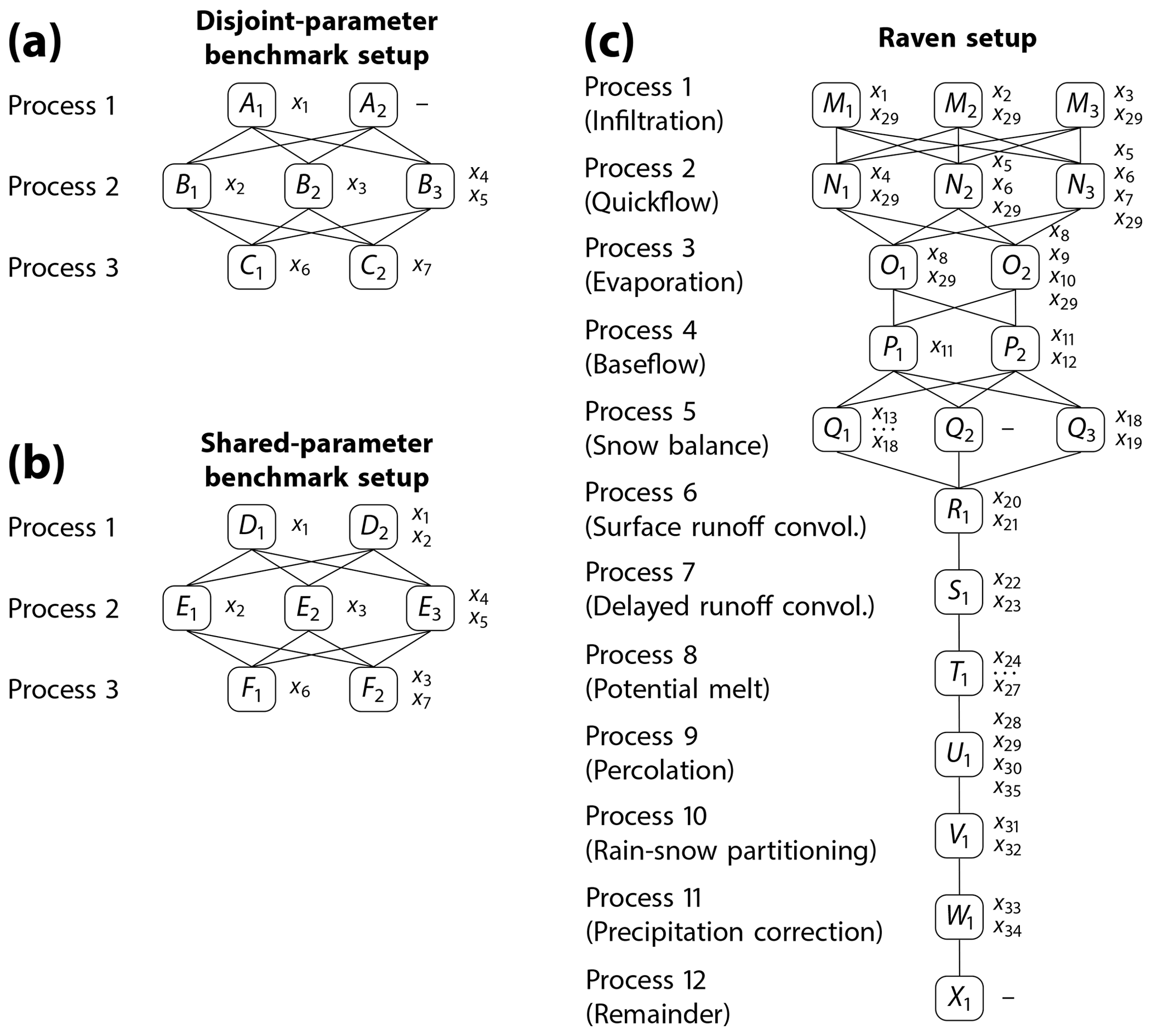
Figure 1The three model setups used in this study. The first two serve as an artificial benchmark model since sensitivities of parameters, process options and processes can be derived analytically. The benchmark examples consist of three processes: A, B, and C (D, E, and F). The three processes are connected through () to obtain the hypothetical model outputs. Processes A (D) and C (F) have two options; process B (E) has three. The parameters xi required for each process option are listed right of the respective process options. Each parameter of the disjoint-parameter benchmark model (a) appears in exactly one process option (disjoint parameters), while in the more advanced benchmark model (b) parameters x1 and x3 appear in multiple process options and processes. The process formulations can be found in Eqs. (3) to (9) and (10) to (16). (c) The third setup is used for a sensitivity analysis of the hydrologic modeling framework Raven. The three options Mi are used for the infiltration process, three options Ni for quickflow, two options Oi for evaporation, two options Pi for baseflow, and three options Qi for snow balance. All other processes needed for the model are used with one fixed option, i.e., convolution for surface and delayed runoff R1 and S1, respectively, potential melt T1, percolation U1, rain–snow partitioning V1, and precipitation correction W1. The remaining processes also have only one option, but none of them contains tunable parameters. They are merged to a “remaining” process X1. The Raven model parameters x1 to x35 are listed right of the process options. Details on the chosen process options can be found in Appendix C Table C1, and details on the model parameters and their ranges are in Appendix C Table C2.
The model that is built using the first process options
resembles the Ishigami–Homma function (Ishigami and Homma, 1990), which is a common benchmark function in sensitivity analysis studies (Homma and Saltelli, 1996; Cuntz et al., 2015; Stanfill et al., 2015; Pianosi and Wagener, 2015, 2018; Mai and Tolson, 2019). The Ishigami–Homma parameters a and b are fixed at 2.0 and 1.0, respectively.
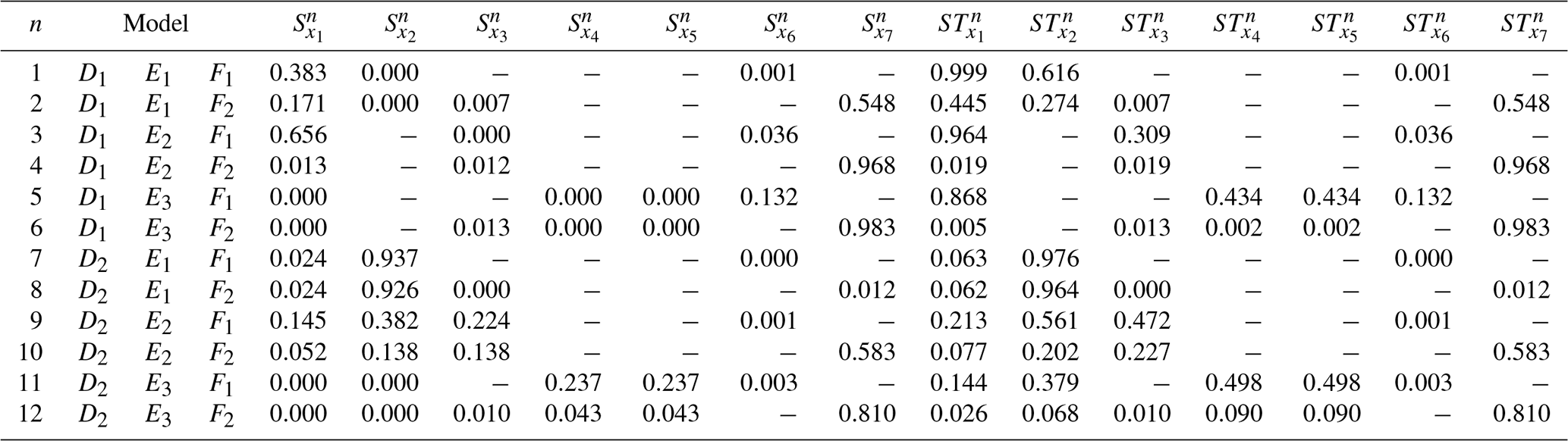
The Sobol' sensitivity indexes of all 12 model configurations can be derived analytically following closely the description in Saltelli et al. (2008) (pp. 179–182). They are listed for the shared-parameter benchmark model in Table B1 of Appendix B.
A reasonable approach for evaluating the sensitivity of 12 individual models involves choosing exactly one process option for each process in Eq. (2), e.g., D=D1, E=E2, and so on. This can be generalized by choosing a weighted sum of all available process options to represent a process, e.g., The sum of weights wi per process is assumed to be 1. In the case of the shared-parameter benchmark example, Eq. (2) therefore changes to
where
The 12 individual models can be obtained when the weights are set accordingly; e.g., the Ishigami–Homma function can be obtained by setting . However, given that weights can take on non-integer values, we now have an infinite number of model structures rather than 12. The same can be constructed for the disjoint-parameter model setup.
To sample the continuum of all process options, the weights need to be independently and identically distributed (iid). Therefore, random numbers ri are sampled from the uniform distribution, 𝒰[0,1], and transformed into the weights following the approach described by Moeini et al. (2011). N−1 such random numbers are required for N weights of competing options. The recipe on how to transform the uniformly sampled numbers ri into weights is specified in Eq. (A1) of Appendix A. For the benchmark example, one requires four such uniform random numbers (r1, …, r4) to derive the seven weights (w1, …, w7).
The approach of weighted model options hence comes at the expense of introducing additional parameters ri to derive the weights. Larger numbers of model parameters always results into an increased number of model runs needed for the sensitivity analysis. However, using the model with weighted options, one now has to run and analyze only one generalized model structure instead of 12 fixed structures. Therefore, this approach reduces the number of required model runs provided that the model allows to derive outputs of weighted process options directly. This feature is available in the hydrologic modeling framework Raven and was the primary reason for the choice of this flexible modeling framework over others. The sensitivities of the additional model parameters (i.e., weights) can further hold interesting insights into the model structure (see Sect. 3).
The analytically derived Sobol' indexes for the remaining three sensitivity metrics (b–d) can be derived using the revised model description (Eq. 18). The indexes for the shared-parameter model setup can be found in Eqs. (B1) to (B3) in Appendix B.
2.1.2 Hydrologic modeling framework Raven
The Raven hydrologic modeling framework developed by James R. Craig at the University of Waterloo (Craig et al., 2020) is a C++ based framework that gives users full flexibility regarding model input handling and hydrologic process description chosen for each process of the water cycle. It is platform independent, open source, and retrievable from http://raven.uwaterloo.ca (last access: 2 December 2020). For this study we used the released version 3.0. The Raven framework currently allows for an ensemble of about 8×10¹² hydrologic model configurations with, for example, 14 options for infiltration, 13 options for percolation, and 9 for baseflow handling. The overall number of model structures is hypothetical as not all processes need to be present in a model setup. For example, the sublimation process allows for six different options in Raven but would likely not be used to model an arid catchment. Further, other processes might appear several times. For example, convolution processes can be defined for each soil layer and hence would increase the number of possible models.
In Raven, the user defines the model as a list of hydrologic processes which move water between storage compartments corresponding to physical stores (e.g., topsoil, canopy, snowpack). The list determines the state variables, connections between stores and the parameters required. For each hydrologic process, several options of process algorithms are implemented. There are, for example, 14 infiltration process options available. Amongst others, the GR4J (Perrin et al., 2003), HMETS (Martel et al., 2017), UBC watershed model (Quick and Pipes, 1977), PRMS (Markstrom et al., 2015), HBV (Bergström, 1995), VIC (Wood et al., 1992), and VIC/ARNO (Clark et al., 2008) infiltration descriptions are implemented. All options of each process can be combined with all options of other processes. Raven can fully emulate a number of hydrologic models (GR4J, HMETS, MOHYSE, HBV-EC, and the UBC Watershed model) by choosing specific configurations of the hydrologic processes.
Raven has another unique feature relative to other modular frameworks: Rather than selecting one process option (e.g., HMETS method for estimation of infiltration runoff fluxes) one can specify multiple process options (e.g., HMETS, VIC/ARNO, and HBV) and define weights for each option (e.g., 0.4, 0.5, and 0.1, respectively). Raven then uses the weighted sum of the fluxes calculated by the process options internally. Raven is run only once and not multiple times to obtain the outputs for the multiple process options. Based on this feature, we chose Raven as model for our study. Please note that the proposed sensitivity method is applicable for any multi-model framework that allows to mix-and-match process descriptions. However, in the case of a framework without weights for process options, the application of the method would be much less efficient.
For the case study used herein, Raven is applied in lumped mode, and the models are solved using the ordered series numerical scheme defined in Craig et al. (2020, end of Sect. 3.2 therein). We have chosen three different options Mi for the infiltration process, three options Ni for quickflow, two options Oi for evaporation, two options Pi for baseflow, and three options Qi for snow balance. All other processes, i.e., convolution for surface runoff R1 and delayed runoff S1, potential melt T1, percolation U1, rain–snow partitioning V1, and precipitation correction W1, are used with one fixed process option. The remaining processes also have only one option, but none of them contains tunable parameters. They are merged to a “remaining” process X1. This remaining process will never appear in the sensitivity analysis because it is constant. Details of process options can be found in Appendix C Table C1.
This selection of process options results in possible models when only one option is allowed per process. When the first option of each process M1, N1, O1, P1, Q1, R1, S1, T1, U1, V1, W1, and X1 is chosen and parameter x35 is set to zero, the Raven setting emulates the HMETS model (Martel et al., 2017) perfectly. All other combinations are unnamed models. The Raven model is stable for all of these combinations, although a check of the hydrologic realism of these models, as done by Clark et al. (2008), was not performed.
Figure 1b shows the possible combinations and associated active parameters. In total, 35 model parameters are active in at least one model option. The details on model parameters and their ranges used for the sampling of parameter sets are listed in Table C2 of the Appendix. An additional number of 13 () weights is required for the weighted model setup (similar to Eq. 18) and is also sampled using the approach described in Appendix A. Therein, 8 () parameters ri are sampled uniformly 𝒰[0,1] and transformed into weights wi.
2.1.3 Case study domain
The Salmon River catchment located in the Canadian Rocky Mountains in British Columbia is selected as the study watershed. The domain is depicted in Fig. 2a and was chosen only for the purpose of demonstrating the proposed method. The catchment drains towards a Water Survey Canada (WSC) streamflow gauge station near Prince George (WSC ID 08KC001; latitude 54.09639∘ N, latitude −122.67972∘ W; elevation 606 m) and has continuous data since 1953. The 4230 km2 large, low-human-impacted catchment is mainly evergreen needleleaf forested (83 % of whole domain) on a loamy (63 %) and loamy sandy (25 %) soil (Fig. 2c and d).

Figure 2(a) Location of the Salmon River catchment (red polygon) in British Columbia, Canada. The watershed is 4230 km2 and located around 700 km north of Vancouver. It is located in the Rocky Mountains with an elevation of 606 m above sea level at the streamflow gauge station of the Salmon River (08KC001). (b) The average monthly mean temperatures (red line) and average monthly precipitation is divided into rain (dark blue) and snow (light blue). Maps of (c) the four soil types based on the Harmonized World Soil Data (HWSD; 30′′) (Fischer et al., 2008) and (d) four land cover types based on the MCD12Q1 MODIS/Terra+Aqua Land Cover (500 m) (Friedl, Sulla-Menashe, Boston University and MODAPS SIPS, NASA, 2015) of the Salmon River catchment are provided. The colors indicate different soil and land use classes.
Meteorological inputs are obtained from Natural Resources Canada on an approximately 10×10 km2 grid. The model is set up in lumped mode. Hence, all available forcing grid points that fall within the catchment have been aggregated. Average daily temperature and the daily sum of precipitation have been used to force the Raven model. The forcings are available from 1954 to 2010. The average annual precipitation of the Salmon River catchment is 592.7 mm over the 57 years of available data. The monthly distribution of precipitation is shown in Fig. 2b, where rain is highlighted as the dark blue portion of each bar and snow as the light blue portion of each bar. The basin has a dryness index (PET/P) of 0.735, which demonstrates the energy limitation of this catchment.
The lumped model was set up for the simulation period from 1 January 1989 to 31 December 2010, while the first 2 years were discarded as warm-up. Hence, 20 years of daily streamflow simulations were used for this study.
2.2 Sensitivity analysis: theory
In this section we briefly describe the Sobol' method (Sobol', 1993) that is traditionally used to derive model parameter sensitivities (Sect. 2.2.1). This corresponds to the sensitivity metric a mentioned in the introduction. To calculate the sensitivity metrics b, c, and d, we propose an extended version of the Sobol' method which is introduced in Sect. 2.2.2.
2.2.1 Traditional Sobol' sensitivity analysis: sensitivities of individual model parameters
Traditionally, the Sobol' sensitivity analysis – as all other methods – focuses on the sensitivity of model parameters. In the case of multiple models, one would typically run the analysis individually for each model and might aggregate the sensitivity index estimates for parameters that are active in multiple models. This, however, may underestimate the sensitivity of parameters that are active in only a few models, while parameters that are active in almost all the models might be overestimated in their aggregated sensitivity.
We here briefly revisit the implementation of the traditional Sobol' method to emphasize the differences with the extended method we propose that will be able to handle multiple process options and derive (overall) parameter sensitivities, sensitivities of process options, and sensitivities of whole processes.
Usually two Sobol' indexes are derived: the main and total Sobol' indexes. The main Sobol' index of a parameter xi regarding a certain model output f(xi) represents the variability in the model output Vi that can be achieved by changing this parameter while keeping all other parameters at a nominal value. This impact is normalized by the overall model variability V(f) that can be generated when all model parameters are varied. Therefore, the main index is derived by
where V depicts variances and E expected values. E(f|xi) is the expected model output when the model parameter xi is fixed.
Similarly, the total Sobol' index for a parameter xi regarding a certain model output f(xi) is similar to the main index but includes parameter interactions. Therefore, it is derived using the variability of model output that can be generated by changing all parameter subsets that include parameter xi. Since there might be a large number of such subsets, the total index for parameter xi can also be viewed as 1 minus the variability that can be achieved by changing all parameters but not parameter xi (V∼i) normalized by the overall possible model output variability Vf:
where V depicts variances and E expected values. is the expected model output when all model parameter except xi are fixed.
Sobol' (1993) proposed an elegant and efficient method to approximate the variances Vi, V∼i, and V(f). We have used the implementations proposed by Cuntz et al. (2015) (Appendix D therein). Unlike derivative-based methods, the Sobol' index calculations are only dependent on the model outputs, but not the parameter values xi.
For the numerical estimation of the indexes and , one samples two base matrices 𝒜 and ℬ which each contain K parameter sets (rows) of N parameters (columns). The samples are assumed to be independent within one matrix and between the matrices. We used the stratified sampling of Sobol' sequences here to improve convergence speed of the derived indexes compared to a Monte Carlo sampling. Based on 𝒜 and ℬ, a set of additional N matrices 𝒞i is constructed. 𝒞i is a copy of 𝒜, but column i is replaced with column i of matrix ℬ. The model then needs to be forced with all the parameter sets; in total, model runs are required, where N is the number of parameters and K is the so-called number of reference parameter sets. K needs to be chosen to be large enough to obtain stable Sobol' indexes. This number is highly dependent on the model, but K=1000 seems to be a good rule of thumb (Cuntz et al., 2015, 2016).
Out of the 12 possible shared-parameter benchmark models (Eq. 2), there are 4 models that contain 3 parameters; 5 models contain 4 parameters, 2 models consist of 5 parameters, and 1 model has 6 parameters. Hence, 72 000 () model runs would be required if K=1000 reference parameter sets are used.
2.2.2 Extended Sobol' sensitivity analysis: sensitivities of groups of model parameters
The Sobol' method is here generalized to groups of parameters xG rather than focusing on individual parameters xi. The subscript G is used here to refer to parameter groups, such that VG represents the variance of a group of parameters xG, e.g., the set . Although the grouping of parameters has previously been used (Sobol' and Kucherenko, 2005; Saltelli et al., 2008; Gilquin et al., 2015), it is – to our knowledge – the first time they have been used to group parameters of process options in the context of examining model structure sensitivity. The calculation of the main and total Sobol' indexes is marginally changed: instead of changing individual parameters, xi groups of parameters get changed. The derivation of the main index gets generalized to
where V depicts variances and E expected values. E(f|xG) is the expected model output when the set of model parameters xG is fixed. This simplifies to Eq. (19) in case the group xG contains exactly one model parameter xi. Similarly, the total Sobol' index can be generalized to
where V depicts variances and E expected values. is the expected model output when all model parameters except the ones in of group xG are fixed. This simplifies to Eq. (20) when the group xG contains only the parameter xi. Note that the groups are not assumed to be mutually exclusive, which means that parameters can appear in multiple groups.
The numerical approximation of these indexes is similar to the traditional approach. It is again based on the two matrices 𝒜 and ℬ containing K parameter sets each. Assuming that the sensitivity of M groups needs to be estimated, M matrices 𝒞m have to be constructed where 𝒞m is a copy of 𝒜 but all columns that correspond to parameters in group m are replaced by the corresponding column of ℬ. For example, if the group consists of parameters x2, x4, and x5, the columns 2, 4, and 5 would be replaced by the columns 2, 4, and 5 of matrix ℬ. The number of model runs that need to be performed is where K is the number of reference parameter sets.
The xSSA method can be used to derive conventional model parameter sensitivities by using groups that contain exactly one of the model parameters xi or random numbers ri that are required to derive weights (sensitivity metric b). It can also supply the sensitivity of process options by defining a group for each process option containing exactly the parameters of that option (sensitivity metric c) or defining a group for each process containing all parameters active in at least one of the process options to derive the sensitivity of whole model processes (sensitivity metric d).
As an example (see Fig. 1b), the group to derive the sensitivity of process option A2 of the shared-parameter benchmark model would contain parameters x1 and x2. The group to determine the sensitivity of process B of this benchmark model would contain parameters x2, x3, x4, and x5.
The shared-parameter benchmark model consists of 7 model parameters xi and 4 random variables ri used to derive the 7 weights wi. Let's assume we used K=1000 reference parameter sets for each of the three analyses. One would require 13 000 () model runs to derive individual parameter sensitivities using the xSSA method. This is compared to the 72 000 model runs required when the conventional Sobol' sensitivity analysis method is applied to the 12 individual models. It requires 13 000 () additional model runs to derive the sensitivity of the seven process options A1, A2, B1, … C2 and 5000 () additional model runs to derive the sensitivity of the three processes A, B, and C. The total of 31 000 model runs for all three analyses thus leads to a computational cost reduction of 57 % while providing additional information about process option and process sensitivity.
2.3 Sensitivity analysis: experiments
Four experiments will be performed for each of the two benchmark models to demonstrate that the proposed method is able to obtain the analytically derived values available for the the benchmark examples (Sect. 2.3.1). Another set of four experiments is performed using the Salmon River catchment model (Sect. 2.3.2). These experiments are performed to demonstrate the type of insights that can be obtained for hydrologic models using the proposed method.
2.3.1 Experiments using the benchmark models
The artificial benchmark models are used to prove that the proposed method of extended Sobol' sensitivity indexes and its implementation is working. They are furthermore employed to demonstrate some limitations of the existing method proposed by Baroni and Tarantola (2014) (discrete value method) to derive sensitivities regarding model structures. The analytically derived values for the traditional approach analyzing the individual 12 models independently (sensitivity metric a) can be found in Appendix B Table B1 for the shared-parameter model setup. The budget of such an analysis is 72×K with K reference parameter sets as described in Sect. 2.2.1. Mai and Tolson (2019) and Cuntz et al. (2015) have demonstrated that these indexes can be obtained with a classical Sobol' analysis for the Ishigami–Homma model. The analytically derived values for the sensitivity metrics b to d of the shared-parameter model are available in Eqs. (B1–B3) of Appendix B. All analytically derived indexes are obtained by following the descriptions in Saltelli et al. (2008, p. 179 ff.).
The xSSA method is tested using different budgets to show that numerical values indeed converge. The number of reference sets used are , 50 000, 100 000}. The budget to derive parameter sensitivities (sensitivity metric b) is for seven parameters xi and four weight-deriving random numbers ri. To derive sensitivities of process options (sensitivity metric c), model runs are required for the seven process options D1, D2, …, F2 and the four weight-deriving random numbers ri. For the analysis of processes (sensitivity metric d), the model needs to be run times to obtain sensitivities of the three processes D, E, and F.
The DVM also applied to the two benchmark models was set up using the same computational budgets K as above. The method requires additionally the definition of the algorithmic parameter ni which denotes the number of realizations for each source of uncertainty Ui analyzed (ni and Ui are terms used in the original publication). The term “sources of uncertainty” (Ui) is used by Baroni and Tarantola (2014) to describe groups of parameters with aggregated sensitivity and is here equivalent to the process groupings A, B, and C for the disjoint-parameter benchmark model and D, E, and F for the shared-parameter benchmark model. Several values for ni were tested (32, 64, 128, 256, 512, 1024). Only results for ni equal to 128, which was used in the original publication (Baroni and Tarantola, 2014), will be reported as all other results appeared to be similar.
The errors between approximated main effects and the analytically derived true indexes as well as errors between the approximated total indexes and its analytically derived truth are reported for both the xSSA and the DVM.
2.3.2 Experiments using the Raven modeling framework
The Salmon watershed model is analyzed using the xSSA method with K=1000 reference parameter sets assuming that this number of parameter sets is large enough to derive stable results. The analysis of individual models (sensitivity metric a) would have required 3 258 000 model runs and is not performed here.
The budget for the sensitivity metric b analyzing unconditional sensitivity of parameters independent of choice of model options results in model runs for the 35 model parameters xi and eight weight-deriving random numbers ri. The budget for process options is model runs for the 19 process options M1, M2, …, W1 and eight weight-deriving random numbers ri. The process X1 is not analyzed since it does not contain any parameters and is hence constant, resulting in a zero sensitivity. The budget for the analysis to obtain process sensitivities is for the 11 processes M, N, …, W.
The sensitivities are determined for simulated streamflow Q(t) for the 20-year simulation period from 1991 to 2010. The main and total Sobol' indexes and , respectively, are determined for each time step t and are aggregated to and using variance-weighted means (Cuntz et al., 2015):
where V(t) is the total variance at time step t.
We further analyze the time-dependent behavior of process sensitivities to reveal temporal patterns in the importance of processes at different times of the year. Therefore, the total process sensitivity STM(t), STN(t), … STW(t) over the 20-year simulation period () is averaged for each process at each day of the year (), resulting in STM(t′), STN(t′), … STW(t′). Sensitivity estimates from leap days are discarded. The sums of sensitivities at each time step are normalized to 1.0 in order to ease the comparison of all time steps:
We will present the results of the extended Sobol' sensitivity analysis (xSSA) applicable not only to model parameters, but also to model process options and processes. First, the xSSA method will be compared to the existing discrete value method (DVM) to derive sensitivities of groups of parameters introduced by Baroni and Tarantola (2014), highlighting limitations of these existing methods (Sect. 3.1). Second, we will present the convergence of the xSSA results regarding parameters, process options, and processes, focusing on the shared-parameter benchmark model (Sect. 3.2). The results of the xSSA for the hydrologic modeling framework are presented in Sect. 3.3.
3.1 Benchmarking against analytically derived solutions and an existing method
In this section the proposed xSSA method based on grouped parameters and weighted process options will be compared against analytically derived Sobol' sensitivity indexes for both benchmark problems (Fig. 1a and b). The xSSA method will also be compared to the sensitivity analysis method introduced by Baroni and Tarantola (2014) (hereafter called the DVM), which also makes use of grouped parameters. Weighted process options are irrelevant for the version of the discrete value method employed by Baroni and Tarantola (2014) as only one “process option” was used in their publication.
The DVM defines the term “sources of uncertainty” (Ui) to describe groups of parameters with aggregated sensitivity and is used here to be equivalent to the process groupings A, B, and C for the disjoint-parameter benchmark model and D, E, and F for the shared-parameter benchmark model. The DVM pre-samples a defined number ni of sets for each “uncertainty source” Ui. Forcing datasets could be one such source of uncertainty. In this case, the DVM pre-samples ni input time series and the Sobol' method would use the ID of the time series (1…ni) as the hyper-parameter to derive the sensitivity of the inputs. In the case of their proposed example, the sources of uncertainty are distinct and the parameterizations of the “sources of uncertainty” are disjoint. The question is how the DVM would be applied if two competing error structures of the same forcings are supposed to be tested, for example, when both error structures shared one or more of the same statistical parameters such as the mean error and error variance, eliminating the disjoint nature of parameters that all past studies using the DVM implicitly assume and utilize. The same question appears in the context of process option sensitivity when a parameter (e.g., porosity) is shared between multiple alternative process options or even multiple processes (e.g., a soil evaporation process option and a percolation process option). The xSSA method is not limited in these situations by using the weighted sum of all competing model options and the definition that parameters are allowed to appear in multiple process options and even in multiple processes.
To demonstrate this major difference of the DVM and the proposed xSSA concept, we define three groups (sources of uncertainty) as the processes A, B, and C of the disjoint-parameter benchmark model (Fig. 1a). For this scenario, all the parameters are disjoint, and it can be shown that both methods converge to the analytically derived Sobol' indexes (Fig. 3a and b).
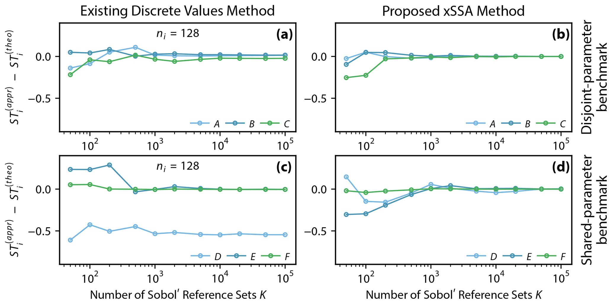
Figure 3Error between approximated and analytically derived total Sobol' sensitivity index estimates for processes of the benchmark models and , respectively. The analyses are performed using increasing numbers of Sobol' reference sets K. The errors are expected to converge to zero for an increasing number of reference sets. The existing discrete value method (DVM) proposed by Baroni and Tarantola (2014) (a, c) is compared to the proposed method xSSA (b, d) using the disjoint-parameter and shared-parameter benchmarking models (Fig. 1a and b, respectively). The model parameters are here grouped to model processes A, B, and C for the disjoint-parameter benchmarking model and D, E, and F for the shared-parameter benchmarking model. The main difference between these two models is that parameters of the latter model can appear in multiple processes (or groups of uncertainty), which is regarded as more realistic. Note that the x axis is in logarithmic scale.
The shared-parameter benchmark model (Fig. 1b), by contrast, has parameters that appear in several process options of the same process (e.g., x1 in A1 and A2) and parameters that are involved in several process options across processes (e.g., x3 in E2 and F2). This non-disjoint (overlapping) setting of influencing factors leads to the result that the DVM converges to a wrong sensitivity for some processes. This is caused by the usage of the ni pre-sampled parameter sets for each source of uncertainty (here processes). When a parameter appears in two sources of uncertainty, one has to make a decision which parameter value to choose for running the model; during the Sobol' analysis (when creating the M matrices 𝒞m) one process expects this parameter to stay constant, while the other assumes it is getting changed. This contradiction cannot be resolved in a method that does not allow for shared parameters. Shared parameters occur often in several process options of the same process but also across processes and hence need to be considered when analyzing process options and processes in flexible frameworks. In this methodology, it is at the user's discretion which parameters are grouped and how they are grouped. A defining characteristic of the xSSA approach is that it can support any grouping of parameters, though interpretation of xSSA results benefits from meaningfully assigning group membership. In our implementation we had chosen to use the parameter value of the last process leading to process F converging to the analytically derived correct value. Process E also converges almost to the correct value, but only because parameter x3 which is shared between processes E and F is very insensitive (STx3=0.0045). Process D shares the highly sensitive parameter x2 (STx2=0.77089) with process E. Thus the sensitivity for process D is significantly underestimated. The underestimation is caused by the fact that the parameter value is supposed to change, but it is kept constant because it gets overwritten by the value of x2 of the pre-sampled set of process E.
We also tested several numbers of pre-sampled parameter sets ni as this is mentioned by Baroni and Tarantola (2014) as one factor that can influence the convergence of the method. We tested ni with 32, 64, 128, 256, 512, and 1024, and all led to the same results (results not shown).
The xSSA method does not pre-sample parameters. When one group is analyzed, all parameters contained in this group get perturbed. The 𝒞m matrices can be defined without causing any contradiction or overwriting of parameter values. The method intrinsically counts repeatedly sensitivities for parameters that appear multiple times. This characteristic of this method is intentional and desirable. When the groups are defined as process options, i.e., various conceptual implementations of the same hydrologic process, parameters will be used in multiple options. Some parameters such as, for example, soil thicknesses or porosity might even be required across processes (for example, infiltration and percolation). We do not expect the process sensitivities to sum up to 1, which is anyway not achievable with non-additive models (Sobol' and Kucherenko, 2005; Saltelli et al., 2008). In addition to the practical benefit of allowing for non-disjoint parameter groups, the theoretical underpinning of analytically derived Sobol' indexes does not require this constraint, as shown with the xSSA results converging towards those values.
It is notable that several publications that are considering structural sensitivities so far have been limited by the disjoint definition of parameter groups (Baroni and Tarantola, 2014; Schürz et al., 2019; Francke et al., 2018; Günther et al., 2019). They would hence show a similar behavior to that presented here for the results of an example discrete value method.
3.2 Extended Sobol' sensitivity analysis for shared-parameter benchmark setup
The shared-parameter benchmark setup is utilized to compare the xSSA-derived numerical sensitivity metric values with the analytically derived, correct sensitivity metric values for all three metrics: parameters, process options, and processes. We have chosen the shared-parameter model over the disjoint-parameter benchmark model here as it appears to be the more difficult model to analyze. The errors converge to zero in every analysis, and this proves that the implementation of the extended Sobol' sensitivity analysis is coherent with the analytical theory (Fig. 4).
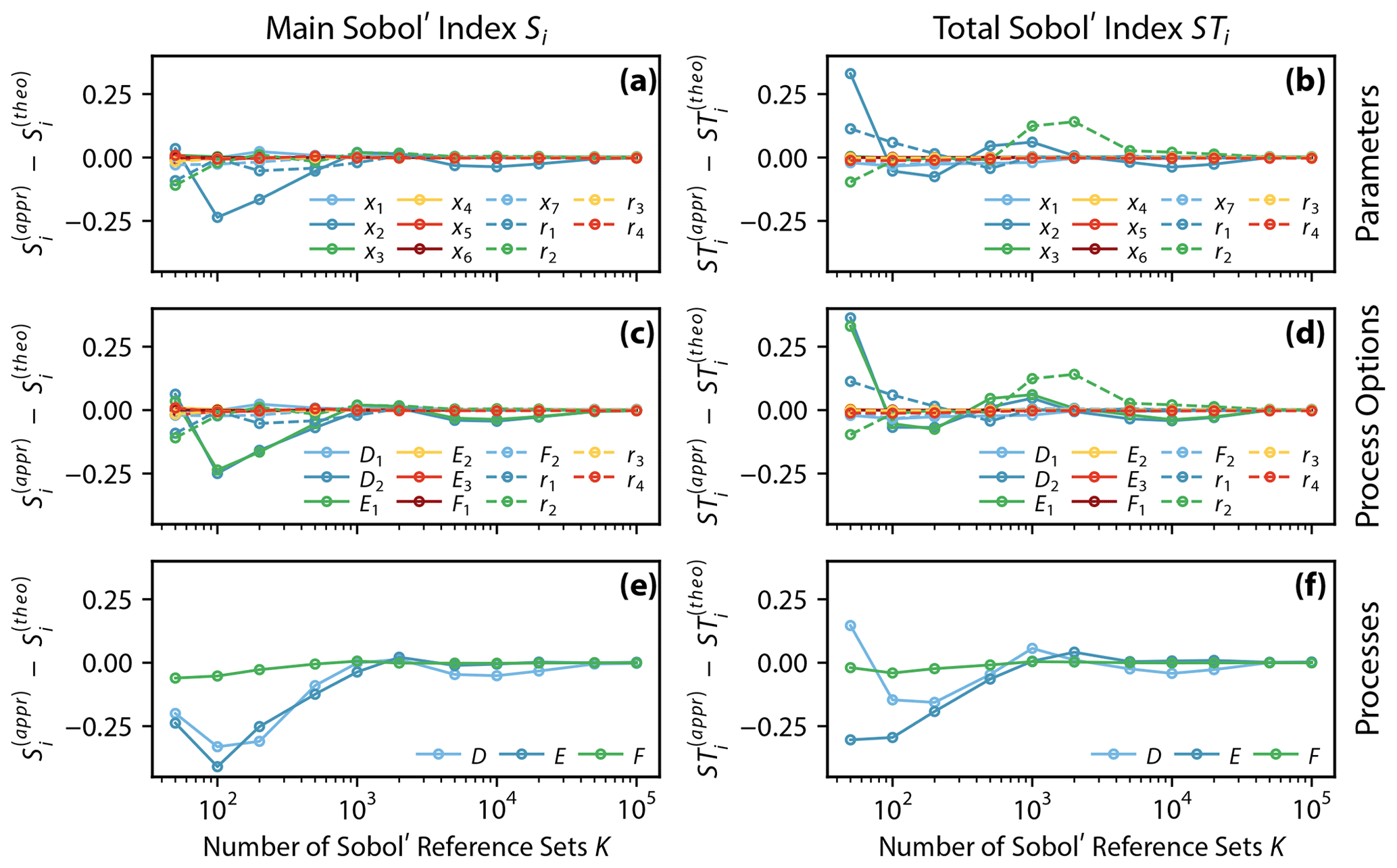
Figure 4Error between xSSA approximated and analytically derived Sobol' sensitivity index estimates and , respectively. The errors are derived for the main Sobol' indexes Si and the total Sobol' indexes STi. The analyses were performed for (a, b) model parameters, (c, d) process options, and (e, f) processes of the shared-parameter benchmark model (Fig. 1b, Eq. 2). The analyses are performed using increasing numbers of Sobol' reference sets K. Note that the x axis is in logarithmic scale. (f) is the same as Fig. 3d.
It holds for all three analyses that the model parameters/options/processes with the largest sensitivities converge slowest. For example, model parameter x2 and weight-generating random number r2 have much higher sensitivities than other parameters analyzed and need about 5000 model runs to obtain an error below 0.1 (Fig. 4a and b). Similarly, Fig. 4c and d show that the most influential process options (D2, E1) and most influential variable (r2) converge slowest (, , , , , ). Process F's sensitivity estimates converge more quickly than the other two, as is consistent with the fact that this process is the least sensitive (Fig. 4e and f).
It can be noted that the weight-generating random numbers ri show high interaction effects – which makes sense since they always couple at least two parameters or process options – and hence tend to converge slower due to the higher sensitivity. In this study we are primarily interested in the model parameter, process option, and process sensitivities and hence suggest that a number of K=1000 model runs is sufficient to derive useful sensitivity estimates.
3.3 Extended Sobol' sensitivity analysis applied to a hydrologic modeling framework
Each subsection here focuses on one experiment performed using the hydrologic modeling framework Raven. The subsections will address the results of the unconditional parameter sensitivities (Sect. 3.3.1), the sensitivities of the process options (Sect. 3.3.2), and the processes (Sect. 3.3.3). All these sensitivity indexes are presented as variance-weighted aggregates over time such that one index per model parameter, option, or process can be analyzed. The last subsection focuses on temporally varying process sensitivities over the course of the year (Sect. 3.3.4), as shown to be of importance previously (Dobler and Pappenberger, 2012; Herman et al., 2013; Günther et al., 2019; Bajracharya et al., 2020).
It is important to note that the results of the analysis for the hydrologic framework are the product of an iterative process where the intermediate results are not quantitatively reported on. Qualitatively, we wish to emphasize that the intermediate xSSA-based results helped us to improve the modeling framework by identifying sources of model instabilities and non-intuitive model results. It was especially helpful to have estimates for aggregated model compartments, i.e., process options and processes. We strongly believe that this kind of analysis will help to analyze the hydrologic realism of models since the estimates are easier to interpret and to compare to experience and known evidence.
3.3.1 (Unconditional) parameter sensitivity
The variance-weighted main and total Sobol' sensitivity estimates and are shown in Fig. 5. The sensitivities are unconditional since the estimates average over all possible model structures through the weighted sum of all analyzed model options as it is described in Eq. (18). The analysis of model parameters (Fig. 5a) shows that the most sensitive ones are x24 to x27, which are all associated with the potential melt (process T) that handles the melting of snowpack until it is gone. The quickflow parameters x5 (maximum release rate from topsoil) and x6 (baseflow rate exponent n of topsoil) are sensitive as well. Parameters of medium sensitivity are x8 (PET correction factor), x16 (degree-day refreeze factor), x18 (refreeze factor), x19 (maximum snow liquid saturation), x29 (thickness of topsoil), x31 (temperature of rain–snow transition), and x34 (snow correction factor).
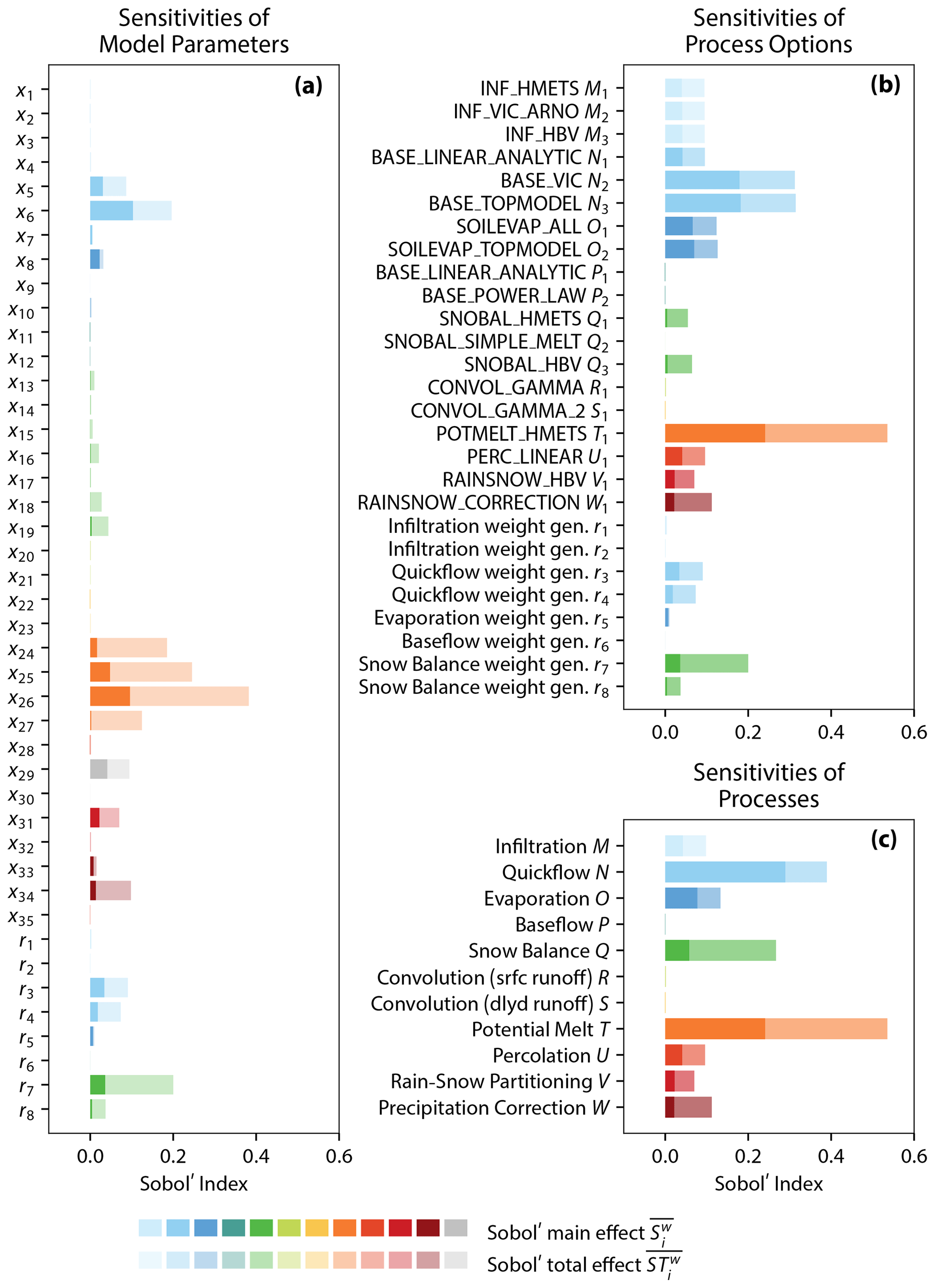
Figure 5Results of the Sobol' sensitivity analysis of the hydrologic modeling framework Raven. (a) The sensitivities of 35 model parameters (see Table C2) and 8 parameters ri that are used to determine the weights of process options are estimated. The Sobol' sensitivity index estimates are determined also for (b) 19 process options and (c) the 11 processes. The information on which parameters are used in which process option and process can be found in Table C1. The different colors indicate the association of parameters and process options with the 11 processes. Parameters x29 and x30 are associated with several process options and are not colored but gray. The Sobol' main and total effects are shown (dark and light colored bars, respectively). All sensitivity index estimates shown are originally time-dependent and are aggregated as variance-weighted averages (Eqs. 23 and 24). The average weights over the course of the year are shown in Fig. 6.
Besides that, the most influential parameters are the weight-generating random variables associated with processes that are most sensitive (indicated by the same color in Fig. 5a), i.e., r3, r4, and r7. This is intuitive since switching processes may cause large variability in the model outputs, and hence shifting their weighted averages is also likely to lead to large variability.
A sensitivity analysis regarding model parameters is often performed prior to model calibration to identify the most sensitive parameters, which are in turn the parameters that are most likely to be identifiable during calibration. The analysis shows that 13 of the 35 parameters (x5, x6, x8, x16, x18, x19, x24, x25, x26, x27, x29, x31, and x34) are responsible for 96.5 % of the overall model variability (only ; 77.2 % if is included). All other parameters are unlikely to be identifiable during model calibration using streamflow measurements alone. Independent of the model structure selected, these model parameters are negligible and thus could be fixed at default values for the Salmon River catchment over the 20-year simulation period.
This analysis helps to identify the most influential parameters independently of model structure and therefore helps to identify the main sources of parametric uncertainty in models despite structural configuration, presuming that individual structures are equally viable. It likewise determines non-identifiable parameters – as a traditional sensitivity analysis does – with respect to streamflow.
3.3.2 Process option sensitivity
The results of the sensitivity analysis of model parameters are consistent with the analysis of process options (Fig. 5b) where all model parameters used in a process option are varied together rather than individually. The analysis of the process option sensitivities identifies options as most sensitive that contain model parameters that have been previously determined to be sensitive.
The potential melt process – the algorithm used to determine incoming melt energy – is used in this study only with one process option (POTMELT_HMETS), and it is still the hydrologic process that the simulated streamflow is most sensitive to (orange bar). The three infiltration options are all equally sensitive (light blue bars). The same holds for the two options of the evaporation process (dark blue bars) which are slightly more influential than the infiltration processes (light blue bars). The quickflow options BASE_VIC and BASE_TOPMODEL (medium blue bars) are the second-most sensitive after the potential melt. The quickflow option BASE_LINEAR_ANALYTIC however is much less sensitive. The two baseflow options (dark green bars) as well as the convolution options for surface and delayed runoff (yellow and light green bars) exhibit almost no influence with sensitivity metrics near zero ( with ). The only percolation option (PERC LINEAR; light red bar), rain–snow partitioning option (RAINSNOW_HBV; medium red bar), and precipitation correction (RAINSNOW_CORRECTION; dark red bar) show medium sensitivities similar to the ones of the infiltration options. The SNOBAL_HBV option is the most sensitive among the three snow balance options. SNOBAL_HMETS is slightly less sensitive, while SNOBAL_SIMPLE_MELT has zero sensitivity. The zero sensitivity is expected since the SNOBAL_SIMPLE_MELT option does not require any parameters (see Table C1). Model outputs of such options do not change for different model runs and hence have a zero variance which leads to a zero Sobol' index. Such settings and parameters that are a priori known to yield zero sensitivities are beneficial in sensitivity analyses as they act as a consistency check of the implementation (Mai and Tolson, 2019). Another interesting result is the high sensitivity of the weight-generating random numbers associated with the snow balance options (r7 and r8). The sensitivity of these parameters is caused by the fact that they are responsible for the “mixing” of the outputs of the model options. In this case they mix a process that is always the same (SNOBAL_SIMPLE_MELT) and two options that can vary significantly with parameter choice (SNOBAL_HBV and SNOBAL_HMETS). Hence, the weighting of these processes can perturb the model output drastically and hence yields a high sensitivity of r7 and r8.
In summary, it can be deduced that the potential melt, the quickflow options BASE_VIC and BASE_TOPMODEL, and the evaporation options are most influential upon modeled streamflow. The interpretation and use of this process option sensitivity is open, and depends upon the purpose of the sensitivity analysis. As an example of interpretation, we can consider whether or not we wish to maximize the flexibility of our models in calibration, and if so, we may wish to discard insensitive processes. The three infiltration options are equally sensitive and hence are all able to achieve the same amount of variability in simulated streamflow time series. This similarity is an indicator that the choice of the infiltration option will therefore not influence the model performance.
This analysis of process options allows us, for the first time, to objectively compare model process options by mixing-and-matching all of them through the approach of a weighted mean of all outputs. It can assist the setup of models by guiding choices of process options and hence guides model structure decisions depending on the purpose of the model built.
3.3.3 Process sensitivity
The sensitivity analysis of the 11 processes (Fig. 5c) consistently identifies potential melt T (orange bar) as the dominating process for the Salmon River catchment. Technically, potential melt T as well as rain–snow partitioning V and precipitation correction W handle inputs to the hydrologic system and can hence be regarded as quantifying input uncertainties or, in other words, are a forcing correction function and do not change the water balance within the model. The three processes are responsible for 42.1 % of the overall model variability in this catchment. Note that the process weights ri, unlike for parameter and process option sensitivities, are not explicitly included in the process sensitivity results in Fig. 5c (unlike Fig. 5a and b). The weights are part of the parameters that get grouped for each process to assess its sensitivity.
Processes associated with the surface are quickflow N and snow balance Q (medium blue and medium green bars, respectively), which are the second- and third-most influential processes. These two processes control together about 38.5 % of the model variability. The strong impact of these processes (together with the input adjustments) highlights the sensitivity of streamflow regarding snow and melting processes in this mountainous, energy-limited catchment.
The soil-related processes of infiltration M, evaporation O, and percolation U show a medium sensitivity (19.2 % of total model variability). This demonstrates that soil and surface processes are of secondary sensitivity regarding streamflow. Their sensitivity may increase if the uncertainty of the snow and melting processes can be reduced, i.e., by narrowing parameter ranges during calibration.
Baseflow P, and the convolution of the surface R and delayed runoff S have almost no influence on the simulated streamflow (control on 0.2 % of overall variability). These three processes demonstrate that subsurface and routing processes are not influential in this catchment over the 20 years simulation period at a daily time step. This in turn leads to the conclusion that even if, for example, additional ground water observations were available, it would not help to reduce model streamflow prediction uncertainty.
This model structure-based sensitivity analysis can help to guide model development by targeting the dominant model processes. It derives a high-level sensitivity of the main model components, i.e., processes. It reveals, for the first time, the sensitivity of model processes independently of model structure chosen and hence is one step towards sensitivity analyses regarding model structure using a true model ensemble by mixing-and-matching a variety of model process options.
3.3.4 Process sensitivity over time
The previous analysis estimated the time-aggregated sensitivities and of model processes 𝒫 (Fig. 5c) which might mask interesting patterns in the temporal sensitivities of streamflow to the 11 processes. We therefore augment the analysis by calculating the normalized total Sobol' sensitivity indexes of each process 𝒫 at every day of the year t′ (Fig. 6). Each value displayed is an average over 20 values – one for each year of the 20-year simulation period. The figure also shows the weights V(t) (Fig. 6, black line) that were used to derive the variance-weighted total Sobol' indexes (Eq. 24) previously discussed using Fig. 5c. The weights are generally higher during the high-flow freshet period (mid February to mid May) and are close to zero for the rest of the year.
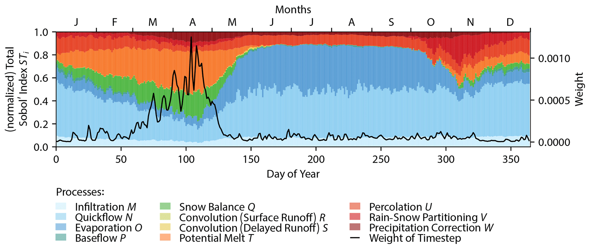
Figure 6Results of the Sobol' sensitivity analysis of the hydrologic modeling framework Raven. The sensitivities of 11 processes are shown as their averages per day of the year (colored bars). The simulation period is 1991 to 2010. The sensitivities are normalized such that they sum up to 1.0 at every day of the year (Eq. 25). The sensitivities are variance-weighted averages (Eq. 24). The (average) weight of each day of the year is shown as a black line. The weights for every time step are determined by the average simulated discharge at this time step (V(t) in Eq. 24). The time-aggregated sensitivity index estimates of the 11 processes are shown in Fig. 5c.
Infiltration (light blue) has an almost constant but minor sensitivity throughout the whole year. Quickflow (medium blue) is most of the time the dominating process – especially in summer – but not during the high-flow melt season. Evaporation (dark blue) is consistently responsible for about 35.4 % of the sensitivity during summer (June to October) and is, expectedly, less sensitive during winter. Snow balance (medium green) and potential melt (orange) are sensitive as long as snow is present (November to May). Potential melt is about twice as influential than snow balance process. Percolation (light red) is almost constant in its sensitivity but nearly negligible. Baseflow (dark green) and the convolution of the surface runoff as well as the delayed runoff (light green and yellow) are not even visible in the graph and have negligible sensitivities throughout the whole year.
These results highlight the importance of the weighting procedure when deriving the aggregated sensitivities shown in Fig. 5. Potential melt (orange) is the most sensitive process when using variance-weighted aggregates due to its dominant influence in the high-flow season. The arithmetic mean of all time-dependent sensitivities Si(t) and STi(t) would have certainly resulted in a much higher sensitivity of the quickflow process which is not as influential during the melting period but is responsible for 41.7 % of the model variability during summer (June to October). The same holds for the evaporation process, which is highly sensitive in summer but not during the melting season.
The traditional method to derive sensitivity index estimates for model parameters conditional on a fixed model structure is of limited applicability when the model is allowed to vary in its structure. First, the number of model runs can be massive when each model is analyzed independently. Second, the analysis derives a unique model-dependent sensitivity index for each parameter but no overall parameter sensitivity across the ensemble. Third, aggregated sensitivities of model processes or the sensitivity of a set of process options may lead to more useful insights than analyzing individual model parameters.
In this work we introduce two new concepts. The first is the idea of reformulating a hydrologic modeling framework such that it is able to weight or blend discrete model process options for simulating process-level fluxes. This converts the countable, discrete model ensemble space into an infinite, continuous model space. The method of weighted process options is shown to significantly reduce the number of model runs required to run a sensitivity analysis based on model parameters. For the shared-parameter benchmark model, 81.9 % fewer model runs are required (A: 72 000 vs. B: 13 000). For the hydrologic model example, the reduction is greater than 98.6 % (A: 3 258 000 vs. B: 45 000). The method of weighted process options derives unconditional sensitivities of the model parameters independently of the model structure.
The second key contribution here is the application of the conventional Sobol' sensitivity analysis method based on grouped parameters and interpreting these groups as process options and hydrologic processes. The extended Sobol' sensitivity analysis (xSSA) method uses these groups of parameters to perturb them simultaneously rather than individually, allowing the simultaneous assessment of model output sensitivity to model parameters, model process options, and model processes. While grouping of parameters is not a new concept for Sobol' analyses, they have to our knowledge not yet been interpreted in the context of sensitivity assessment to model structural choices. The method was successfully tested using two artificial benchmark models based upon the Ishigami–Homma function. The estimated sensitivity indexes are proven to converge against the analytically derived Sobol' sensitivity indexes for model parameters, process options, and processes. The xSSA method is shown to resolve limitations of an existing method that also derives sensitivities of groups of parameters but that cannot handle overlapping parameter groupings.
The extended Sobol' sensitivity analysis method was also applied to a hydrologic modeling framework that supports the representation of internal model fluxes using a weighted sum of fluxes calculated from individual process algorithms/options. The sensitivity analysis of the hydrologic modeling framework used here identified potential melt processes and other surface processes as the most influential processes regarding streamflow in a mountainous, energy-limited, and snow-dominated catchment, while all subsurface and routing processes were insensitive. This information helps to guide further model development and model calibration and can inform the incorporation of additional observations to reduce model uncertainty. Three processes (potential melt, rain–snow partitioning, precipitation correction) handle solely inputs to the hydrologic system and can hence be attributed as input uncertainty or, in other words, model components adjusting forcing functions.
The presented methods of weighted process options and the application of the extended Sobol' sensitivity analysis method present a simultaneous analysis of model structure, model parameters, and forcing adjustments in a frugal way consistent with known methods based on the Sobol' method.
In this work we define a model that uses the weighted average of a set of process options instead of choosing one fixed process option (Eq. 18). This enables one to analyze several model structures at the same time by either setting weights to 0 or 1 (which selects exactly one option) or any weight in between, which leads to the weighted average of those process option outputs.
The sampling of such weights needs to lead to independent and identical (not necessarily uniform) distribution for each of the weights wi. We use the sampling strategy introduced by Moeini et al. (2011) which can be summarized as follows: for each set of N+1 weights needed, first generate a vector of random numbers (r1, r2, …, rN) from a uniform distribution between 0 and 1. The corresponding vector of weights (w1, w2, …, wN+1) can then be calculated using
with
This sampling leads to the following CDF FN and PDF fN for each of the N+1 weights wi:
Python and R implementations of the sampling algorithm of Eq. (A1) are freely available on https://github.com/julemai/PieShareDistribution (last access: 2 December 2020).
All sensitivity indexes for the benchmark setups (Sect. 2.1.1) are obtained by following the descriptions in Saltelli et al. (2008, p. 179 ff.). We provide the results for the shared-parameter benchmark (Eq. 2 with Eqs. 10 to 16) in the following.
The analytically derived sensitivity indexes of sensitivity metric a are given in Table B1 using Ishigami–Homma parameters a=2.0 and b=1.0. The values are given for each of the 12 models that can be built using the different process options of the artificial benchmark model.
The analytically derived results of the overall parameter sensitivities (independent of the model options chosen; metric b), the sensitivities of process options (metric c), and sensitivities of processes (metric d) are listed in Eqs. (B1), (B2), and (B3), respectively. The parameters ri therein are the random variables required to derive the weights wi of the process options according to Eq. 18 using the sampling strategy described in Appendix A. r1 is used to derive the weights wd1 and wd2, r2 and r3 are used to derive the weights we1, we2 and we3, and r4 is used to derive the weights wf1 and wf2.
Table B1Analytically derived Sobol' indexes Si and STi of the shared-parameter benchmark model with three processes D, E, and F that allow for multiple process descriptions (Eqs. 2 and 10–16). For example, process D has two options: D1 and D2. The model output f(x) is assumed to be to mimic additive and multiplicative model structures. The model corresponds to the Ishigami–Homma function (Ishigami and Homma, 1990). The parameters a and b of the Ishigami–Homma function are set to 2.0 and 1.0, respectively. A dash (−) in the table indicates that the parameter is not active in the respective model.
The Raven hydrologic modeling framework (Craig et al., 2020) has been employed for this study. We used the released version 3.0 of Raven. The process options M1, M2, …, X1 selected for this study are listed in Table C1. The model parameters active in the individual process options are given in that table as well. In total, 35 model parameters are used in at least one of the model options. The valid ranges and parameter descriptions are given in Table C2. Further details about the process option implementation and the parameters can be found in the Raven documentation (Craig, 2020).
Table C1Processes and process options used for the Raven setup. In total models are possible. The first option of each process M1, N1, O1, P1, Q1, R1, S1, T1, U1, V1, W1, and X1 resemble the HMETS model if parameter x35 is set to zero. All other combinations are artificial models. All process options, however, are used in different hydrologic models. The model parameters active in each option are listed as well. The ranges and a description of the parameters can be found in Table C2.
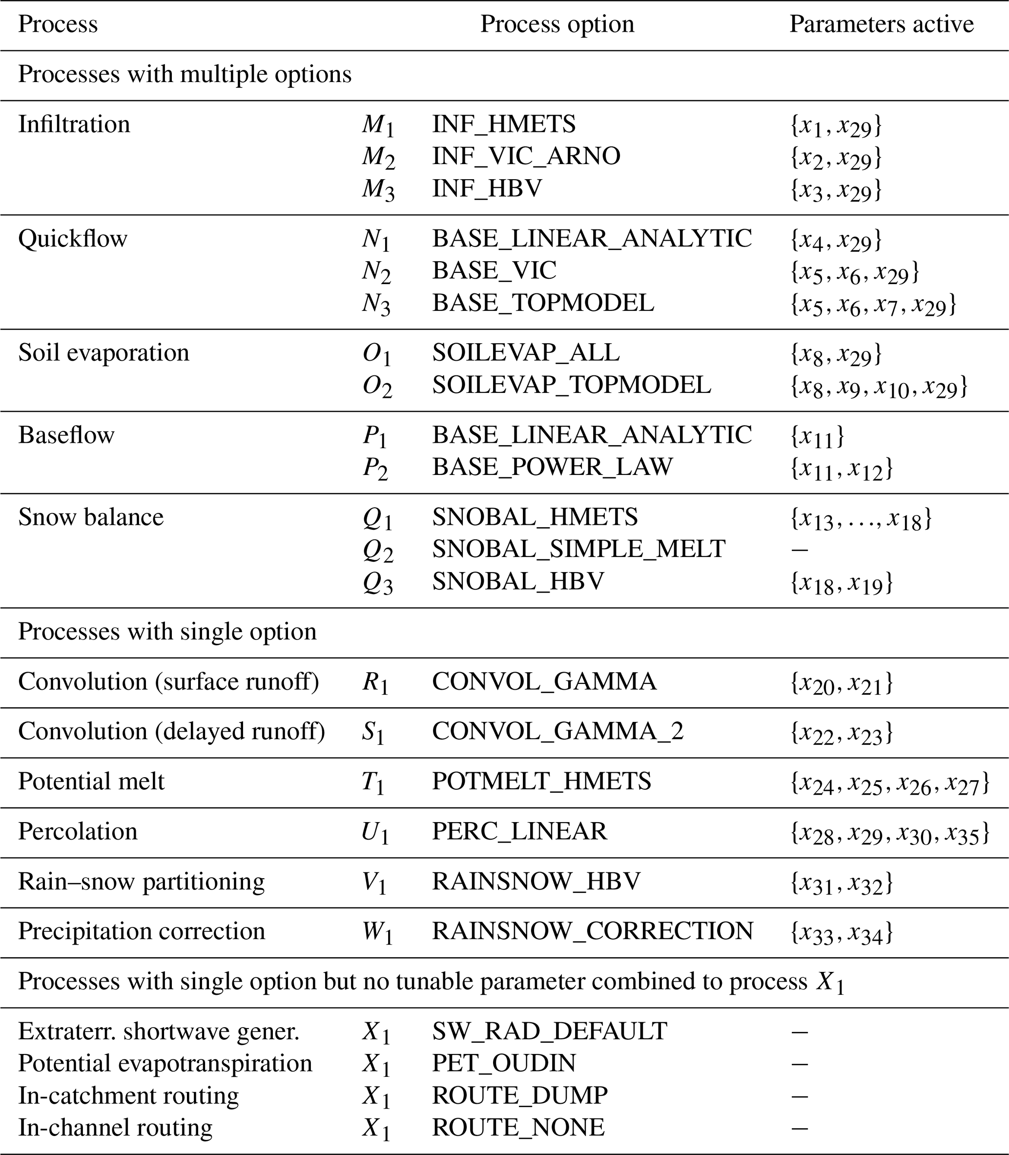
Table C2The model parameters xi used for the Raven setup. The parameters are uniformly distributed in the range given. The process option shows where the corresponding parameter is active. The Raven table and parameter name can be used to locate the parameter in the Raven setup files. A three-layer soil model was used here with the third (groundwater) layer being of infinite depth. The TOPSOIL is the upper soil layer, while PHREATIC is the lower soil layer. The three Raven parameters FIELD_CAPACITY TOPSOIL, SNOW_SWI_MAX, and MAX_MELT_FACTOR are derived using a sampled parameter (x10, x14, and x25) and SAT_WILT TOPSOIL, SNOW_SWI_MIN, and MIN_MELT_FACTOR, respectively, to make sure that one parameter is always larger than the other. The baseflow coefficients BASEFLOW_COEFF TOPSOIL and PHREATIC are derived from parameters x4 and x11 to allow for a logarithmic sampling.
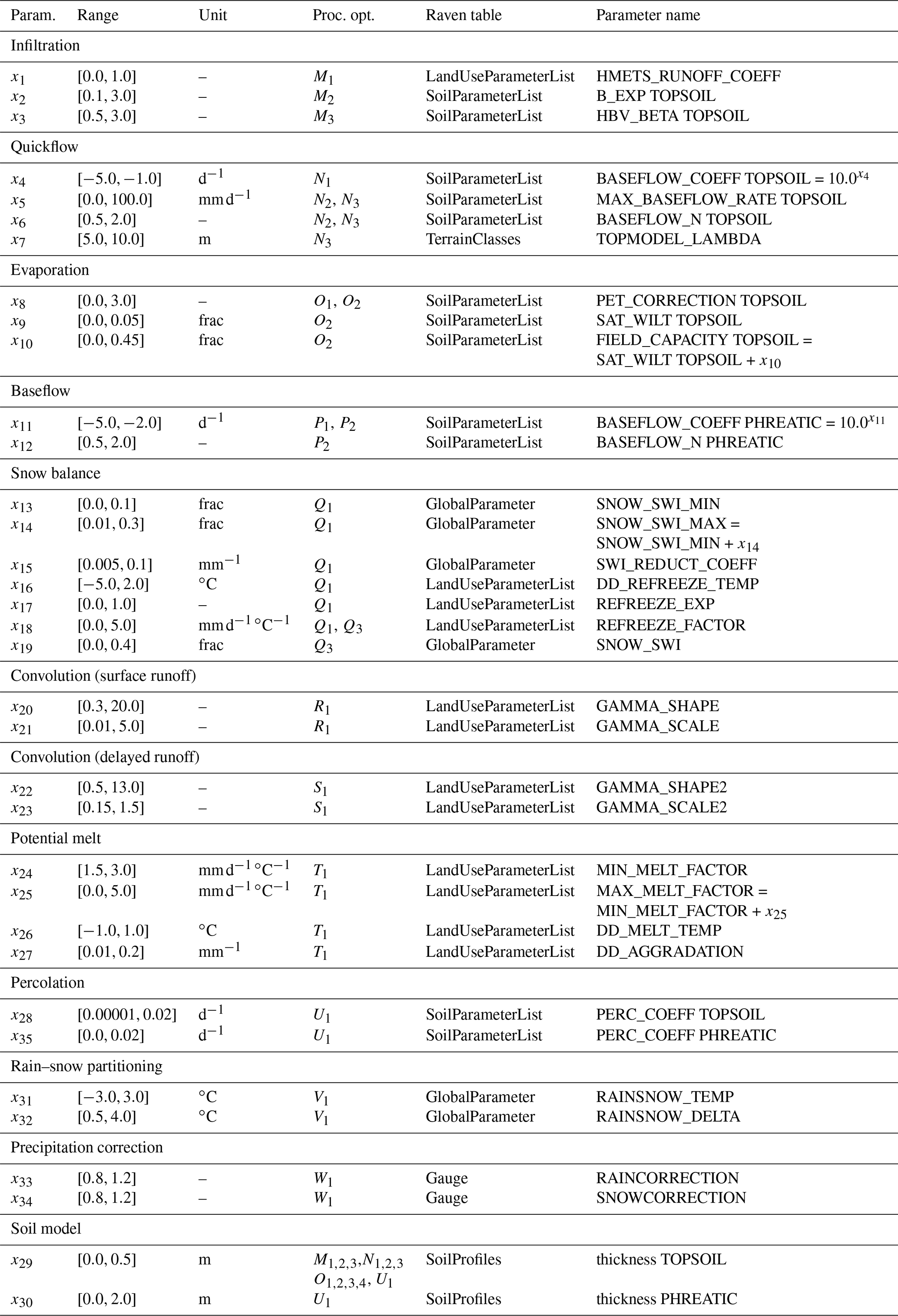
The code and data used for this analysis will be made available on GitHub (https://github.com/julemai/xSSA, https://doi.org/10.5281/zenodo.4301003, Mai and Craig, 2020) upon publication of the paper.
The supplement related to this article is available online at: https://doi.org/10.5194/hess-24-5835-2020-supplement.
JM set up the analyses, implemented the sensitivity analysis based on groups of parameters, implemented the proper sampling of weights used in this study, wrote the main parts of the manuscript, and prepared all figures and tables; JRC contributed to the writing of the manuscript, implemented the weighting of process options in Raven, provided ranges for the parameters included in the analysis, helped to set up the model with the selected options and resolved inconsistencies in Raven detected by earlier versions of the sensitivity analysis, and helped with the hydrologic interpretation of the results; BAT contributed to the writing of the manuscript, provided feedback on the manuscript and the setup of all experiments, including the benchmark models, as well as helped with the hydrologic interpretation of the results.
The authors declare that they have no conflict of interest.
This research was undertaken thanks in part to funding from the CANARIE research software funding program (project RS-332). The work was made possible by the facilities of the Shared Hierarchical Academic Research Computing Network (SHARCNET; https://www.sharcnet.ca, last access: 2 December 2020) and Compute/Calcul Canada. The authors also thank the Canadian Foundation for Innovation John Evans Leaders Fund for the additional supercomputing support and resources. All codes, examples, and data used for this study can be found on GitHub (https://github.com/julemai/xSSA) upon publication.
This research was undertaken thanks in part to funding from the CANARIE research software funding program (project RS-332).
This paper was edited by Jim Freer and reviewed by two anonymous referees.
Abily, M., Bertrand, N., Delestre, O., Gourbesville, P., and Duluc, C.-M.: Spatial Global Sensitivity Analysis of High Resolution classified topographic data use in 2D urban flood modelling, Environ. Model. Softw., 77, 183–195, 2016. a
Bajracharya, A., Awoye, H., Stadnyk, T., and Asadzadeh, M.: Time Variant Sensitivity Analysis of Hydrological Model Parameters in a Cold Region Using Flow Signatures, Water, 12, 961, https://doi.org/10.3390/w12040961, 2020. a
Baroni, G. and Tarantola, S.: A General Probabilistic Framework for uncertainty and global sensitivity analysis of deterministic models: A hydrological case study, Environ. Model. Softw., 51, 26–34, 2014. a, b, c, d, e, f, g, h, i, j, k, l
Bergström, S.: The HBV model, in: Computer Models of Watershed Hydrology, edited by Singh, V., Water Resources Publications, Highlands Ranch, CO, USA, 443–476, 1995. a
Borgonovo, E., Lu, X., Plischke, E., Rakovec, O., and Hill, M. C.: Making the most out of a hydrological model data set: Sensitivity analyses to open the model black-box, Water Resour. Res., 53, 7933–7950, 2017. a
Campolongo, F., Saltelli, A., and Cariboni, J.: From screening to quantitative sensitivity analysis. A unified approach, Comput. Phys. Commun., 182, 978–988, 2011. a
Clark, M. P., Slater, A. G., Rupp, D. E., Woods, R. A., Vrugt, J. A., Gupta, H. V., Wagener, T., and Hay, L. E.: Framework for Understanding Structural Errors (FUSE): A modular framework to diagnose differences between hydrological models, Water Resour. Res., 44, W00B02, https://doi.org/10.1029/2007WR006735, 2008. a, b, c
Clark, M. P., Kavetski, D., and Fenicia, F.: Pursuing the method of multiple working hypotheses for hydrological modeling, Water Resour. Res., 47, 5468–16, 2011. a
Clark, M. P., Nijssen, B., Lundquist, J. D., Kavetski, D., Rupp, D. E., Woods, R. A., Freer, J. E., Gutmann, E. D., Wood, A. W., Brekke, L. D., Arnold, J. R., Gochis, D. J., and Rasmussen, R. M.: A unified approach for process-based hydrologic modeling: 1. Modeling concept, Water Resour. Res., 51, 2498–2514, 2015. a
Craig, J. R.: Raven: User's and Developer's Manual v3.0, available at: http://raven.uwaterloo.ca/files/v3.0/RavenManual_v3.0.pdf, last access: 2 December 2020. a
Craig, J. R., Brown, G., Chlumsky, R., Jenkinson, W., Jost, G., Lee, K., Mai, J., Serrer, M., Snowdon, A. P., Sgro, N., Shafii, M., and Tolson, B. A.: Flexible watershed simulation with the Raven hydrological modelling framework, Environ. Model. Softw., 129, 104728, https://doi.org/10.1016/j.envsoft.2020.104728, 2020. a, b, c, d, e
Cuntz, M., Mai, J., Zink, M., Thober, S., Kumar, R., Schäfer, D., Schrön, M., Craven, J., Rakovec, O., Spieler, D., Prykhodko, V., Dalmasso, G., Musuuza, J., Langenberg, B., Attinger, s., and Samaniego, L.: Computationally inexpensive identification of noninformative model parameters by sequential screening, Water Resour. Res., 51, 6417–6441, 2015. a, b, c, d, e, f
Cuntz, M., Mai, J., Samaniego, L., Clark, M. P., Wulfmeyer, V., Branch, O., Attinger, S., and Thober, S.: The impact of standard and hard-coded parameters on the hydrologic fluxes in the Noah-MP land surface model , J. Geophys. Res.-Atmos., 121, 10676–10700, 2016. a, b
Dai, H., Ye, M., Walker, A. P., and Chen, X.: A new process sensitivity index to identify important system processes under process model and parametric uncertainty, Water Resour. Res., 53, 3476–3490, 2017. a
Demaria, E. M., Nijssen, B., and Wagener, T.: Monte Carlo sensitivity analysis of land surface parameters using the Variable Infiltration Capacity model, J. Geophys. Res., 112, 1–15, 2007. a
Dobler, C. and Pappenberger, F.: Global sensitivity analyses for a complex hydrological model applied in an Alpine watershed, Hydrol. Process., 27, 3922–3940, 2012. a
Evin, G., Thyer, M., and Kavetski, D.: Comparison of joint versus postprocessor approaches for hydrological uncertainty estimation accounting for error autocorrelation and heteroscedasticity, Water Resour. Res., 50, 1–26, 2014. a
Fenicia, F., Kavetski, D., and Savenije, H. H. G.: Elements of a flexible approach for conceptual hydrological modeling: 1. Motivation and theoretical development, Water Resour. Res., 47, W11510, https://doi.org/10.1029/2010wr010174, 2011. a
Fischer, G., Nachtergaele, F., Prieler, S., van Velthuizen, H. T., Verelst, L., and Wiberg, D.: Global Agro-ecological Zones Assessment for Agriculture (GAEZ 2008), IIASA, Laxenburg, Austria and FAO, Rome, Italy, 2008. a
Foglia, L., Hill, M. C., Mehl, S. W., and Burlando, P.: Sensitivity analysis, calibration, and testing of a distributed hydrological model using error-based weighting and one objective function, Water Resour. Res., 45, 1–18, 2009. a
Francke, T., Baroni, G., Brosinsky, A., Foerster, S., López-Tarazón, J. A., Sommerer, E., and Bronstert, A.: What Did Really Improve Our Mesoscale Hydrological Model? A Multidimensional Analysis Based on Real Observations, Water Resour. Res., 54, 8594–8612, 2018. a, b
Freeze, R. A. and Harlan, R. L.: Blueprint for a physically-based, digitally-simulated hydrologic response model, J. Hydrol., 9, 237–258, 1969. a
Friedl, M., Sulla-Menashe, D., Boston University and MODAPS SIPS, NASA: MCD12Q1 MODIS/Terra+Aqua Land Cover Type Yearly L3 Global 500m SIN Grid, NASA LP DAAC, https://doi.org/10.5067/MODIS/MCD12Q1.006, 2015. a
Gilquin, L., Prieur, C., and Arnaud, E.: Replication procedure for grouped Sobol' indices estimation in dependent uncertainty spaces, Inform. Inference – J. IMA, 4, 354–379, 2015. a, b
Green, W. H. and Ampt, G. A.: Studies on Soil Physics, J. Agric. Sci., 4, 1–24, https://doi.org/10.1017/S0021859600001441, 1911. a
Günther, D., Marke, T., Essery, R., and Strasser, U.: Uncertainties in Snowpack Simulations – Assessing the Impact of Model Structure, Parameter Choice, and Forcing Data Error on Point-Scale Energy Balance Snow Model Performance, Water Resour. Res., 55, 2779–2800, 2019. a, b, c
Gupta, H. V., Clark, M. P., Vrugt, J. A., Abramowitz, G., and Ye, M.: Towards a comprehensive assessment of model structural adequacy, Water Resour. Res., 48, W08301, https://doi.org/10.1029/2011WR011044, 2012. a
Haghnegahdar, A., Razavi, S., Yassin, F., and Wheater, H.: Multicriteria sensitivity analysis as a diagnostic tool for understanding model behaviour and characterizing model uncertainty, Hydrol. Process., 31, 4462–4476, 2017. a
Herman, J. D., Kollat, J. B., Reed, P. M., and Wagener, T.: From maps to movies: high-resolution time-varying sensitivity analysis for spatially distributed watershed models, Hydrol. Earth Syst. Sci., 17, 5109–5125, https://doi.org/10.5194/hess-17-5109-2013, 2013. a
Homma, T. and Saltelli, A.: Importance measures in global sensitivity analysis of nonlinear models, Reliab. Engin. Syst. Safe., 52, 1–17, 1996. a
Ishigami, T. and Homma, T.: An importance quantification technique in uncertainty analysis for computer models, in: First International Symposium on Uncertainty Modelling and Analysis (ISUMA'90), 3–5 December 1990, pp. 398–403, IEEE, University of Maryland, College Park, MD, 1990. a, b
Mai, J. and Craig, J. R.: julemai/PieShareDistribution: PieShareDistribution v1.0 (Version v1.0), Zenodo, https://doi.org/10.5281/zenodo.4300332, 2020. a
Mai, J. and Tolson, B. A.: Model Variable Augmentation (MVA) for Diagnostic Assessment of Sensitivity Analysis Results, Water Resour. Res., 55, 2631–2651, 2019. a, b, c
Markstrom, S. L., Regan, R. S., Hay, L. E., Viger, R. J., Webb, R. M., Payn, R. A., and LaFontaine, J. H.: PRMS-IV, the Precipitation-Runoff Modeling System, Version 4., in: US Geological Survey Techniques and Methods, U.S. Department of the Interior, U.S. Geological Survey, Reston, Virginia, Book 6, chapt. B7, p. 158, 2015. a
Martel, J.-L., Demeester, K., Brissette, F., Poulin, A., and Arsenault, R.: HMETS – A Simple and Efficient Hydrology Model for Teaching Hydrological Modelling, Flow Forecasting and Climate Change Impacts, Int. J. Engin. Educ., 33, 1307–1316, 2017. a, b
McMillan, H., Freer, J., Pappenberger, F., Krueger, T., and Clark, M.: Impacts of uncertain river flow data on rainfall-runoff model calibration and discharge predictions, Hydrol. Process., 47, 1270–1284, 2010. a
McMillan, H., Krueger, T., and Freer, J.: Benchmarking observational uncertainties for hydrology: rainfall, river discharge and water quality, Hydrol. Process., 26, 4078–4111, 2012. a
Moeini, A., Abbasi, B., and Mahlooji, H.: Conditional Distribution Inverse Method in Generating Uniform Random Vectors Over a Simplex, Commun. Stat.-Simul. Comput., 40, 685–693, 2011. a, b
Morris, M. D.: Factorial sampling plans for preliminary computational experiments, Technometrics, 33, 161–174, 1991. a
Perrin, C., Michel, C., and Andréassian, V.: Improvement of a parsimonious model for streamflow simulation, J. Hydrol., 279, 275–289, 2003. a
Pfannerstill, M., Guse, B., Reusser, D., and Fohrer, N.: Process verification of a hydrological model using a temporal parameter sensitivity analysis, Hydrol. Earth Syst. Sci., 19, 4365–4376, https://doi.org/10.5194/hess-19-4365-2015, 2015. a
Pianosi, F. and Wagener, T.: A simple and efficient method for global sensitivity analysis based on cumulative distribution functions, Environ. Model. Softw., 67, 1–11, https://doi.org/10.1016/j.envsoft.2015.01.004, 2015. a, b
Pianosi, F. and Wagener, T.: Distribution-based sensitivity analysis from a generic input-output sample, Environ. Model. Softw., 108, 197–207, 2018. a
Quick, M. C. and Pipes, A.: U.B.C. WATERSHED MODEL/Le modèle du bassin versant U.C.B, Hydrol. Sci. Bull., 22, 153–161, https://doi.org/10.1080/02626667709491701, 1977. a
Rakovec, O., Hill, M. C., Clark, M. P., Weerts, A. H., Teuling, A. J., and Uijlenhoet, R.: Distributed Evaluation of Local Sensitivity Analysis (DELSA), with application to hydrologic models, Water Resour. Res., 50, 409–426, 2014. a
Razavi, S. and Gupta, H. V.: A new framework for comprehensive, robust, and efficient global sensitivity analysis: 2. Application, Water Resour. Res., 52, 440–455, 2016a. a
Razavi, S. and Gupta, H. V.: A new framework for comprehensive, robust, and efficient global sensitivity analysis: 1. Theory, Water Resour. Res., 52, 423–439, 2016b. a
Saltelli, A., Ratto, M., Andres, T. H., Campolongo, F., Cariboni, J., Gatelli, D., Saisana, M., and Tarantola, S.: Global sensitivity analysis. The primer, John Wiley and Sons, Ltd., Chichester, West Sussex, England, 2008. a, b, c, d, e, f
Schürz, C., Hollosi, B., Matulla, C., Pressl, A., Ertl, T., Schulz, K., and Mehdi, B.: A comprehensive sensitivity and uncertainty analysis for discharge and nitrate-nitrogen loads involving multiple discrete model inputs under future changing conditions, Hydrol. Earth Syst. Sci., 23, 1211–1244, https://doi.org/10.5194/hess-23-1211-2019, 2019. a, b, c
Sobol', I. M.: Sensitivity analysis for non-linear mathematical models, Math. Model. Comput. Exp., 1, 407–414, 1993. a, b, c
Sobol', I. M. and Kucherenko, S. S.: Global Sensitivity Indices for Nonlinear Mathematical Models. Review, Wilmott Mag., 1, 56–61, 2005. a, b, c
Stanfill, B., Mielenz, H., Clifford, D., and Thorburn, P.: Simple approach to emulating complex computer models for global sensitivity analysis, Environ. Model. Softw., 74, 140–155, 2015. a
Van Hoey, S., Seuntjens, P., van der Kwast, J., and Nopens, I.: A qualitative model structure sensitivity analysis method to support model selection, J. Hydrol., 519, 3426–3435, 2014. a
Wood, E. F., Lettenmaier, D. P., and Zartarian, V. G.: A land-surface hydrology parameterization with subgrid variability for general circulation models, J. Geophys. Res., 97, 2717–2728, 1992. a
- Abstract
- Introduction
- Materials and methods
- Results and discussion
- Conclusions
- Appendix A: Generating weights
- Appendix B: Analytically derived Sobol' sensitivities of the shared-parameter benchmark model
- Appendix C: Details on Raven process options and parameters
- Code and data availability
- Author contributions
- Competing interests
- Acknowledgements
- Financial support
- Review statement
- References
- Supplement
The requested paper has a corresponding corrigendum published. Please read the corrigendum first before downloading the article.
- Article
(3468 KB) - Full-text XML
- Corrigendum
-
Supplement
(310 KB) - BibTeX
- EndNote
- Abstract
- Introduction
- Materials and methods
- Results and discussion
- Conclusions
- Appendix A: Generating weights
- Appendix B: Analytically derived Sobol' sensitivities of the shared-parameter benchmark model
- Appendix C: Details on Raven process options and parameters
- Code and data availability
- Author contributions
- Competing interests
- Acknowledgements
- Financial support
- Review statement
- References
- Supplement