the Creative Commons Attribution 4.0 License.
the Creative Commons Attribution 4.0 License.
 | 24 Nov 2020
Variability in epilimnion depth estimations in lakes
Harriet L. Wilson
Ana I. Ayala
Ian D. Jones
Alec Rolston
Don Pierson
Elvira de Eyto
Hans-Peter Grossart
Marie-Elodie Perga
R. Iestyn Woolway
Eleanor Jennings
The epilimnion is the surface layer of a lake typically characterised as well mixed and is decoupled from the metalimnion due to a steep change in density. The concept of the epilimnion (and, more widely, the three-layered structure of a stratified lake) is fundamental in limnology, and calculating the depth of the epilimnion is essential to understanding many physical and ecological lake processes. Despite the ubiquity of the term, however, there is no objective or generic approach for defining the epilimnion, and a diverse number of approaches prevail in the literature. Given the increasing availability of water temperature and density profile data from lakes with a high spatio-temporal resolution, automated calculations, using such data, are particularly common, and they have vast potential for use with evolving long-term globally measured and modelled datasets. However, multi-site and multi-year studies, including those related to future climate impacts, require robust and automated algorithms for epilimnion depth estimation. In this study, we undertook a comprehensive comparison of commonly used epilimnion depth estimation methods, using a combined 17-year dataset, with over 4700 daily temperature profiles from two European lakes. Overall, we found a very large degree of variability in the estimated epilimnion depth across all methods and thresholds investigated and for both lakes. These differences, manifesting over high-frequency data, led to fundamentally different understandings of the epilimnion depth. In addition, estimations of the epilimnion depth were highly sensitive to small changes in the threshold value, complex thermal water column structures, and vertical data resolution. These results call into question the custom of arbitrary method selection and the potential problems this may cause for studies interested in estimating the ecological processes occurring within the epilimnion, multi-lake comparisons, or long-term time series analysis. We also identified important systematic differences between methods, which demonstrated how and why methods diverged. These results may provide rationale for future studies to select an appropriate epilimnion definition in light of their particular purpose and with awareness of the limitations of individual methods. While there is no prescribed rationale for selecting a particular method, the method which defined the epilimnion depth as the shallowest depth, where the density was 0.1 kg m−3 more than the surface density, may be particularly useful as a generic method.
- Article
(3057 KB) - Full-text XML
-
Supplement
(415 KB) - BibTeX
- EndNote


The “epilimnion depth”, “mixed layer”, or “top of the metalimnion” are common terms in limnology, typically referring to the deepest point of the surface layer of a stratified lake, which is characterised as quasi-uniform in terms of physical and biogeochemical properties and overlying a layer of steep vertical gradients. Incoming heat to a lake, received at the lake surface, expands water above 3.98 ∘C, resulting in density stratification. Convective cooling at the surface and mechanical energy injected by the wind drive vertical mixing (Wüest and Lorke, 2003). These competing surface fluxes result in a warm well-mixed layer of water that interacts dynamically with the atmosphere (Monismith and MacIntyre, 2009). The vertical propagation of energy manifested at the lake surface is constrained by the steep density gradients in the metalimnion, which act to decouple the epilimnion from the deep hypolimnion. As such, it has become foundational in limnology to consider a stratified lake as consisting of three well-defined layers: a turbulent epilimnion (diffusivity typically 10−5 to 10−2 m2 s−1), the stable metalimnion ( to 10−6 m2 s−1), and the quiescent hypolimnion ( to 10−4 m2 s−1) (Wüest and Lorke, 2009). The discretisation of these layers, however, is understood to be essentially theoretical, since micro-profile studies show that the conditions within layers are not uniform and exact cut-offs between layers do not necessarily exist (Imberger, 1985; Jonas et al., 2003; Tedford et al., 2014; Kraemer, 2020). The definition of the epilimnion depth is thus inherently subjective but has profound importance in limnology.
Quantifying the vertical extent of the epilimnion is crucial for understanding many of the physical, chemical, and biological processes in lakes. Although the epilimnion is differentiated from the typically shallower layer that is actively mixing (Gray et al., 2020), the depth of the epilimnion indicates the volume and properties of the water that is influenced by air–water interactions. It is therefore essential for interpreting the physical response of lakes to long-term atmospheric changes (Lorbacher et al., 2006; Persson and Jones, 2008; Flaim et al., 2016) and extreme climatic events (Jennings et al., 2012; Calderó-Pascual et al., 2020), and it is even required for predicting the local climate for very large lakes (Thiery et al., 2015). The epilimnion depth is also critical for the estimation of algal light availability, nutrient fluxes, and epilimnetic water temperatures, which determine photosynthesis rates and establish the basis of the food web in a lake (MacIntyre, 1993; Diehl et al., 2002; Berger et al., 2006; Bouffard and Wüest, 2018). The depth of the epilimnion is also used for estimating the transfer of oxygen, received at the lake surface, to deeper layers, sustaining aerobic life and preventing anoxia (Foley et al., 2012; Schwefel et al., 2016).
The increasing availability of high-frequency measured and simulated data, coupled with collaborative networks of lake scientists, offers a great potential for broadening our understanding of the epilimnion depth. Water temperature profile data collected at frequent intervals on automatic monitoring buoys in lakes are becoming increasingly available (Jennings et al., 2012; de Eyto et al., 2016; Marcé et al., 2016). In addition, the collation of these datasets globally through collaborative initiatives such as GLEON (http://gleon.org/, last access: 19 November 2020) and NETLAKE (https://www.dkit.ie/netlake, last access: 19 November 2020) (Weathers et al., 2013; Jennings et al., 2017) and modelling initiatives such as ISIMIP2b (Ayala et al., 2020) broaden the potential for long-term multi-lake studies. However, these datasets also introduce new challenges for estimating metrics such as the epilimnion depth. Such large quantities of data can limit a user's capacity to examine individual profiles and therefore require robust automated algorithms with low computational expense (Read et al., 2011; Pujoni et al., 2019).
Despite the ubiquity of the epilimnion depth, there is no consistent determining method used in limnology. The epilimnion depth can be defined in terms of many variables (e.g. water temperature, water density, turbulence estimations, surface fluxes, biogeochemical properties), represents different temporal scales of variability (e.g. inter-annual to sub-daily), and can be calculated using a range of numerical approaches (e.g. sigmoidal functions, threshold algorithms) (Brainard and Gregg, 1996; Thomson and Fine, 2003; Kara et al., 2003; De Boyer et al., 2004; Lorbacher et al., 2006; Gray et al., 2020). A particularly common approach in limnology, due to the availability of the required data, is to define the epilimnion using water temperature profile data. However, inconsistencies exist between studies which use water temperature (e.g. Zorzal-Almeida et al., 2017; Strock et al., 2017) or water density (e.g. Read et al., 2011; Obrador et al., 2014). Often the epilimnion depth is defined as the location where the change in water temperature or density exceeds a defined threshold. However, studies vary in the value selected which may be defined in absolute units (e.g. Andersen et al., 2017) or gradients between consecutive sensors (e.g. Lamont et al., 2004). A particularly prevalent method in recent studies is the “meta.top” function proposed in the R package “rLakeAnalyzer” (Read et al., 2011). In contrast, epilimnion depth definitions based on actual turbulence measurements are uncommon. Compared with long-term water temperature datasets, there are relatively few turbulent eddy diffusivity measurements in lakes, typically using micro-profiling methods conducted over a small time period (e.g. Imberger, 1985; Tedford et al., 2014). Other methods of estimating vertical eddy diffusivity, from water temperature data, e.g. the Jassby and Powell (1975) heat-flux method, are restricted to use below the epilimnion and photic zone. Vertical turbulence profiles, however, as well as water temperature profiles, are estimated by some hydrodynamic lake models (Goudsmit et al., 2002, Dong et al., 2019). Such modelled data, therefore, offer a tool for assessing commonly used water temperature- or density-based methods in comparison to turbulence-based methods.
The diversity of epilimnion depth definitions and arbitrary selection process suggest that methods may be used interchangeably and are relatively insensitive to the threshold value used. However, recent studies have begun to recognise large inconsistencies between different definitions and the potential problems this may cause, although, so far in limnology, analysis has been restricted to a small number of manual profiles (Gray et al., 2020) and a limited number of methods (Pujoni et al., 2019). Although lower temporal resolution data are sufficient for investigating seasonal patterns, high-frequency data can be used to gain information on the level of day-to-day variability in epilimnion depth and demonstrate how methods perform over a continuum of water column conditions. In addition, through the vast number of measured profiles, high-frequency data offer a more robust comparison of methods than that previously demonstrated with manually collected datasets; even when aggregated to the daily time step, high-frequency data are more representative of the sub-daily variability (Marcé et al., 2016). Given the potential of multi-lake comparison and longitudinal studies, methods are required to perform consistently across temporal and spatial ranges rather than being tailored specifically to one lake or period of time. Therefore, the sensitivity of different methods to temporal and spatial characteristics, such as water column structure and vertical resolution of data measurements, is essential for assessing which methods are most suitable for future analysis (Fee et al., 1996; Thomson and Fine, 2003; Lorbacher et al., 2006; Pujoni et al., 2019).
In this study, we undertook an in-depth comparison of methods commonly used for the estimation of epilimnion depth using high-frequency multi-year data for water temperature profiles, collected with automated monitoring buoys from two European lakes: Lough Feeagh (Ireland) and Erken lake (Sweden). In addition to estimates based on these measured data, we used simulated data output from a lake model to compare water-temperature- and turbulence-based methods and to assess the influence of vertical sensor resolution. The objectives of this study were to (1) compare water-temperature- and water-density-based estimates of the epilimnion depth; (2) compare a range of common methods and threshold values; (3) assess the sensitivity of individual methods to the threshold value, the water column structure, and the vertical sensor resolution; and (4) to compare profile-based methods to turbulence-derived estimates using lake modelled data.
2.1 Study sites
We used data from two European temperate lakes, Lough Feeagh (53∘56′ N, 9∘34′ W) in Ireland and Erken lake (59∘51′ N, 18∘36′ E) in Sweden (Fig. 1). The lakes differ in many characteristics, including depth, surface area, and sensor deployment resolution, providing an opportunity to assess method performance in different lake-specific conditions. Lough Feeagh is located on the west coast of Ireland and is a cold monomictic, oligotrophic, and humic lake with a surface area of 3.9 km2, maximum depth of 45 m, and mean depth of 14.5 m (de Eyto et al., 2016). Erken lake is located in east central Sweden near the Baltic coast and is a dimictic, mesotrophic, clear lake with a surface area of 24 km2, maximum depth of 21 m, and mean depth of 9 m (Yang et al., 2016). In addition, Erken lake has a substantially greater mean summer top–bottom density gradient (0.056 kg m−3 m−1) compared to Lough Feeagh (0.016 kg m−3 m−1).
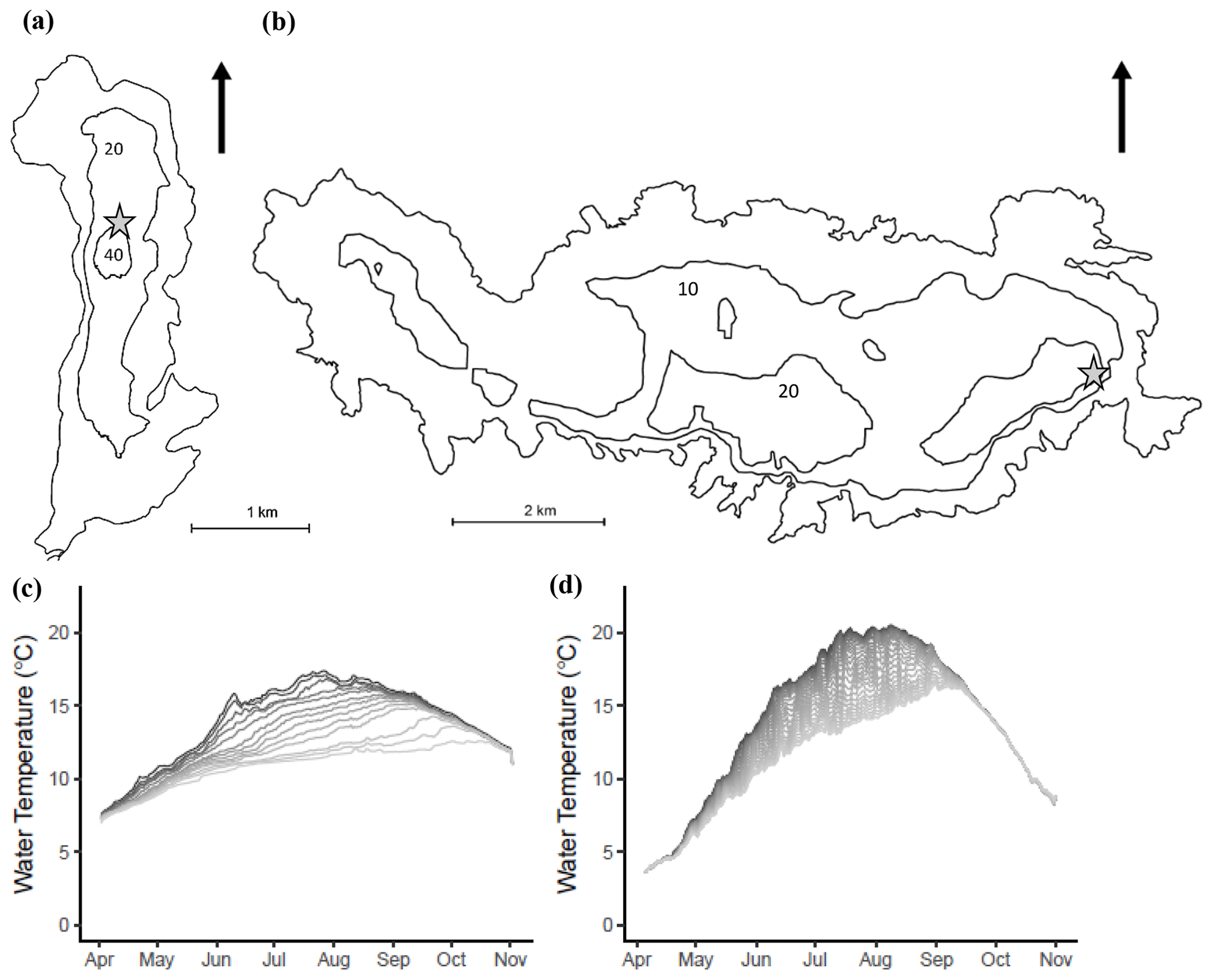
Figure 1Bathymetric map of Lough Feeagh in Ireland (a) and Erken lake in Sweden (b), where the grey stars show the locations of the automatic monitoring buoys used for measuring high-frequency water temperature profiles in both lakes. Long-term mean water temperatures for each Julian day for all measured depths are shown for Lough Feeagh (profiles = 2778, years = 10) (c) and Erken lake (profiles = 2005, years = 7) (d).
2.2 Measured data
In this study, we used a total of 4783 daily water temperature profiles from Lough Feeagh (n=2778) and Erken lake (n=2005). Profiles were collected at frequent intervals on moored automatic monitoring buoys, and from these the mean daily profiles were calculated. On Lough Feeagh, vertical water temperature measurements were collected every 2 min for the period 2004–2017 at depths of 0.9, 2.5, 5, 8, 11, 14, 16, 18, 20, 22, 27, 32, and 42 m using submerged platinum resistance thermometers (PRTs) (PT100 1/10DIN, Lab Facility, Bognor Regis, United Kingdom) (de Eyto et al., 2016, 2020). On Erken, temperature profile data were collected at 1 min intervals at depths of 0.5 to 15 m in 0.5 m intervals, using Type T thermocouple sensors using a Campbell Scientific AM416 multiplexer and CR10 data logger (Pierson et al., 2011). The topmost sensor data were excluded to match the topmost sensor in Lough Feeagh. In Erken lake, the monitoring buoy was manually deployed each year prior to or just after the onset of stratification to avoid damage from the seasonal ice cover; therefore, the number of observations varied annually. To ensure data were consistent for both lakes, data were divided into a subset from 1 April to 31 October. To address the issue of large data gaps, years when less than 70 % of the data between April and October were available (>150 d) were excluded from the analysis. The remaining years were 2004, 2005, 2006, 2011, 2012, 2013, 2014, 2015, 2016, and 2017 for Lough Feeagh and 2002, 2005, 2008, 2009, 2014, 2015, and 2017 for Erken lake. Water density (kg m−3) was calculated from water temperature (∘C) using rLakeAnalyzer (Read et al., 2011), with the Martin and McCutcheon (1999) equation, assuming negligible effects of soluble material.
Meteorological data were required to drive a physical hydrodynamic model (GOTM, Global Ocean Turbulence Mode; Burchard et al., 1999), including wind speed (m s−1), atmospheric pressure (hPa), air temperature (∘C), relative humidity (%), cloud cover (dimensionless, 0–1), short-wave radiation (W m−2), and precipitation (mm d−1). For Erken lake, air temperature, wind speed, and short-wave radiation were collected from the Malma Island meteorological station on the lake at 1 min intervals and averaged to 60 min intervals. Mean sea level pressure, relative humidity, and precipitation were measured at the Svanberga meteorological station located 400 m from the lake shore at 60 min intervals. Cloud cover was recorded from Svenska Högarna station, located 69 km south-east of Erken lake. At Lough Feeagh, wind speed, air temperature, short-wave radiation, mean sea level pressure, relative humidity, and precipitation were measured in the meteorological station next to the lake (de Eyto et al., 2020). Cloud cover was recorded at Knock Airport, located 50 km east from Lough Feeagh.
2.3 Simulated data
The Global Ocean Turbulence Model (GOTM), adapted for use in lakes, simulates small-scale turbulence and vertical mixing (Burchard et al., 1999; Sachse et al., 2014; Moras et al., 2019; Ayala et al., 2020) and was used to simulate daily profiles of water temperature (∘C) and vertical eddy diffusivity (m−2 s−1) for Erken lake and Lough Feeagh. GOTM was calibrated using 4 years of data (2006–2009 for Erken lake and 2008–2011 for Lough Feeagh), including 1-year spin-up followed by 3 years of calibration. The calibrated model parameters were surface heat-flux factor (shf_factor), short-wave radiation factor (swr_factor), wind factor (wind_factor), minimum turbulent kinetic energy (k_min), and e-folding depth for visible fraction of light (g2) (see Table S1 in the Supplement for the calibrated values). During calibration, the model was run approximately 5000 times to obtain a stable solution. The validation period was 7 years for Erken lake (2010–2016) and 4 years for Lough Feeagh (2012–2015). For both the calibration and validation, daily mean water temperatures were simulated when GOTM was forced using measured mean hourly data. Model simulated profiles of mean daily water temperature were then compared to measured mean daily water temperature profiles. Model performance was evaluated by comparing mean daily modelled and measured temperature profiles, and the model efficiency coefficients used were percent relative error (PRE), root mean squared error (RMSE), and Nash–Sutcliffe efficiency (NSE) (Nash and Sutcliffe, 1970). Overall, there was a good model fit for both lakes (Table 1).
Table 1Lake model performance evaluation, showing the percentage relative error (%), root mean squared error (∘C), and Nash–Sutcliffe efficiency for Lough Feeagh (profiles = 1016, years = 5) and Erken lake (profiles = 1449, years = 7).
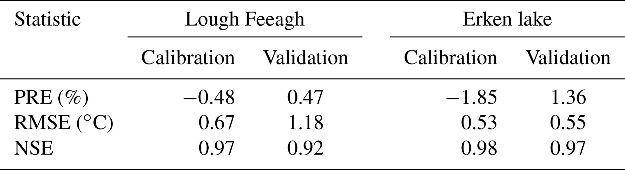
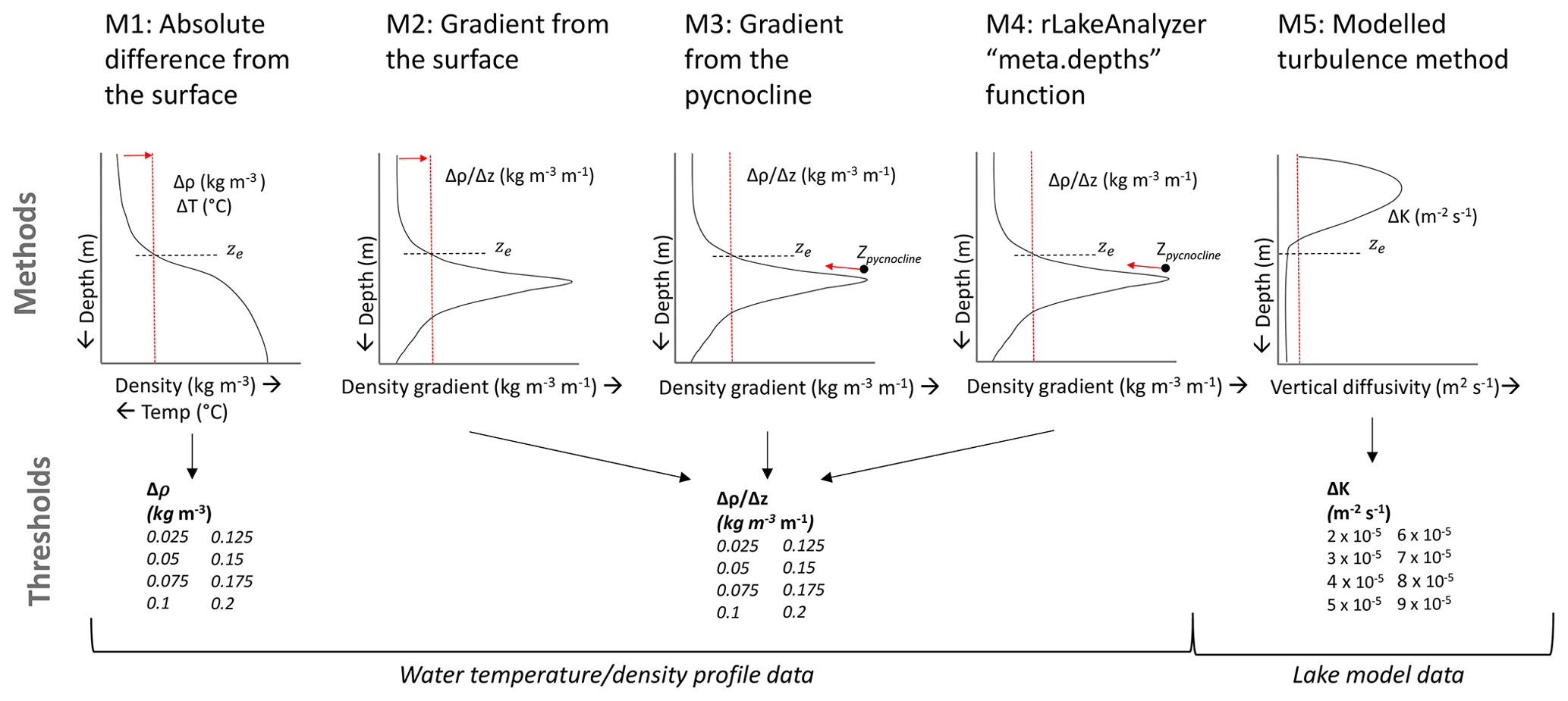
Figure 2Schematic of epilimnion depth methods used in this study, including the range of threshold values for each method and the input data type (i.e. water temperature, density profile, or lake modelled data).
2.4 Definitions for the epilimnion depth
We selected four epilimnion depth definitions that are commonly used in limnology and were computationally efficient for multi-year automated high-frequency data. These methods we describe as profile-based methods (M1–M4) (Fig. 2). In addition, we calculated epilimnion depth using a method for modelled data only (M5). In our analysis, epilimnion depth was expressed relative to the water surface and is therefore always a negative value. The range of thresholds used for each method was selected based on the values found within the literature (see Table 1 in Gray et al., 2020). We made no assumption of the conditions below the deepest measured depth; therefore, the deepest estimated epilimnion depth was limited to the maximum measured depth for each lake (42 m in Lough Feeagh and 15 m in Erken lake).
2.4.1 Absolute difference from the surface method (M1)
In M1, the epilimnion depth was defined as the shallowest depth where the density was a given “threshold” value more than the surface density (Fig. 2), with the surface density (ρ1) approximated as the density at the topmost sensor deployment: 0.9 m in Lough Feeagh and at 1 m in Erken lake. We used a linear interpolation method to estimate the epilimnion depth on a continuous depth scale for all methods (Read et al., 2011), which assumed a linear relationship of densities between the first measured depth which exceeded the threshold (zi+1) and the preceding measured depth (zi). The numerical scheme can be described (using notation from Read et al., 2011) as follows:
where z is depth (m), ρ is water density (kg m−3), and Δρ is the threshold value (kg m−3). The threshold values for the absolute method, M1 only, ranged from 0.025 to 0.2 kg m−3 at intervals of 0.025 kg m−3. For all methods excluding the rLakeAnalyzer method (M4), if the threshold value was not exceeded, the epilimnion depth was defaulted to the deepest value (Lorbacher et al., 2006). Epilimnion depth estimates calculated with water temperature used the same type of equation (Eq. 1) but with temperature rather than density and noting that temperature decreases with depth. The only threshold value used for temperature was 1 ∘C.
2.4.2 Gradient from the surface method (M2)
In M2, the epilimnion depth was defined as the shallowest depth where the density gradient between consecutively measured depths exceeded the threshold value. M2 can be described as
where ziΔ is the midpoint between zi and zi+1, is the density gradient between zi and zi+1, and Δρ∕Δz is the threshold value (kg m−3 m−1). The threshold values for all gradient methods (i.e. M2–M4) ranged from 0.025 to 0.2 kg m−3 m−1 at intervals of 0.025 kg m−3 m−1.
2.4.3 Gradient from the pycnocline method (M3)
In M3, the epilimnion depth was defined as the deepest depth where the density between consecutively measured depths exceeded the threshold value, starting from the depth of the maximum density gradient (hereafter the “pycnocline”) as the reference depth and moving to successively shallower measured depths. M3 can be described by
2.4.4 rLakeAnalyzer (M4)
In M4, the epilimnion depth was defined using the rLakeAnalyzer function “meta.depths” (relating to output “meta.top”), which used the same numerical scheme as M3, Eq. (3), but differed in certain assumptions (Read et al., 2011). Firstly, in M4, the epilimnion depth was prohibited from extending below the depth of the pycnocline. Therefore, for profiles where the predefined threshold value was less than the maximum density gradient, the epilimnion depth defaulted to the maximum density gradient. This differed from the other methods where, for such profiles, the epilimnion depth was defaulted to the deepest measured depth. Secondly, a user-defined filter (“mixed.cutoff” object) was used to remove profiles which were not sufficiently stratified to identify an epilimnion depth. We used the default filter value, which removed profiles where the overall water temperature range was less than 1 ∘C. For the days which did not meet the filter value (and no epilimnion depth was identified), we set the epilimnion depth to the deepest measured depth (i.e. no epilimnion depth) to ensure each method had the same number of data points for comparison with other methods.
2.4.5 Modelled turbulence method (M5)
The modelled turbulence method (M5) used the GOTM lake model simulated profile estimates of vertical eddy diffusivity (m2 s−1). In M5, the epilimnion depth was defined as the first depth, from the lake surface, where the vertical eddy diffusivity fell below the predefined threshold value, and it was described as
where Kz is vertical eddy diffusivity (m2 s−1) and ΔKz is the threshold value (m2 s−1). The thresholds ranged from 10−5 to 10−4 m2 s−1 at intervals of 10−5 m2 s−1, based on the values described in Wüest and Lorke (2009) and MacIntyre and Melack (2009).
2.5 Analysis methods
2.5.1 Comparison between a water-temperature- and water-density-derived methods
To compare water-temperature- and water-density-based estimates of the epilimnion depth, we used M1 only and used a water temperature threshold of 1 ∘C with a density threshold of 0.1 kg m−3 for both sites. Firstly, we investigated the relationship between 1 ∘C and 0.1 kg m−3 throughout the year. To do this, we calculated the long-term mean water column temperature for each Julian day. For each day, we then calculated the change in density that would result from a 1 ∘C increase in the water temperature and then subtracted 0.1 kg m−3. Positive values indicated that a 1 ∘C increase in the water temperature resulted in a greater than 0.1 kg m−3 change in water density, while negative values indicated a less than 0.1 kg m−3 change in water density. Secondly, we compared water-temperature- and water-density-based estimates of the epilimnion depth. To do this, we calculated the difference between the mean water-density-derived estimate and the water-temperature-derived estimate for each Julian day. Positive differences indicated that the water-density-derived estimate was shallower than the water-temperature-derived estimate, while negative values were deeper. For all analyses of measured data, the total numbers of observations were used for Lough Feeagh (n=2778, years = 10) and Erken lake (n=2005, years = 7).
2.5.2 Comparison between water-density-based methods (M1–M4)
Following this, we compared water-density-based epilimnion depth estimates, using all four methods (M1–M4) and the range of thresholds described earlier. Using data from both sites, we considered overall variability (i.e. how much do estimates vary between all methods and all thresholds), variability within each individual method using different threshold definitions (i.e. how sensitive are estimates to the threshold value selected), and variability between methods (i.e. what systematic differences exist between pairs of methods). Given that we had a total of 32 time series to compare, 4 methods each with 8 threshold values, it was necessary to compute summary statistics for each of them. Therefore, the following statistics were calculated for all 32 time series, for the period from 1 April to 31 October each year, and then averaged across all years. Firstly, we calculated the mean epilimnion depth and presented the values for all methods and all threshold values. We also summarised these statistics for each method, showing the mean, standard error of mean, minimum (shallowest), maximum (deepest) and interquartile range for each method, to demonstrate differences between methods. A large interquartile range in epilimnion depth estimates indicated high sensitivity to the threshold value. Secondly, we calculated the percentage of days with available data, when the epilimnion depth was detected above the deepest measured depth. This demonstrated differences between methods in regards to the stratified period. Thirdly, we calculated the percentage of days with available data when the epilimnion depth was detected above the maximum density gradient or pycnocline. By definition the epilimnion should have relatively small density gradients and should not be equal or deeper than the pycnocline; however, automated methods have been found to regularly encroach on the metalimnion (Lorbacher et al., 2006). We therefore used this metric to investigate how frequently epilimnion depth estimates calculated by each method erroneously extended into the metalimnion.
Pearson's correlation coefficients were also calculated for all possible combinations between the 32 time series to quantify the degree of association between them, without using any estimates of significance (Thomson and Fine, 2003; Rivetti et al., 2017). The full correlation matrices were calculated and then for, clarity, we presented only the mean Pearson's correlation coefficient for each method, representing the mean correlation for all possible combinations between threshold values. This indicated the extent to which changing the threshold value influenced the temporal patterns. We also presented the mean Pearson's correlation coefficients between each pair of methods (e.g. for all threshold combinations between M1 and M2) to demonstrate method agreement.
2.5.3 Sensitivity of epilimnion depth to water column structure and vertical sensor resolution
We also assessed the sensitivity of the profile-based methods to changes in the water column structure and the vertical sensor resolution of measured data. For the water column structure sensitivity analysis, we calculated the long-term mean epilimnion depth estimate for each Julian day for all 32 method/threshold time series. For each method, using all thresholds, we calculated the range for each Julian day. The range in estimates was presented alongside the top–bottom density gradient for each Julian day to investigate whether threshold sensitivity varied temporally and with water column structure. For the vertical sensor deployment resolution sensitivity analysis, we compared simulated water density profiles for both lakes at two different resolutions. High-resolution data were resolved to 0.5 m for both lakes. Low-resolution data were subset to a mean of one sensor per 3 m, using the measured depths for Lough Feeagh and data from 1, 2.5, 5, 8, and 13 m for Erken lake. We then calculated the difference between the April–October mean epilimnion depth for the high- and low-resolution data. Methods where the high- and low-resolution data produced very different estimates were regarded as having high sensitivity to the vertical resolution of the data, while methods with small differences indicated low sensitivity. For all analyses using simulated data, the total numbers of observations were used for Lough Feeagh (n=1016, years = 5) and Erken lake (n=1449, years = 7).
2.5.4 Comparison with modelled turbulence method (M5)
Finally, we assessed how each profile-based method compared against the turbulence-based estimates. For this analysis, both water density and vertical eddy diffusivity profile data were derived by using the GOTM lake model. Then, using the same procedures as the measured data, we calculated the mean April–October epilimnion depth for each method. We then calculated the difference between the turbulence method (M5) and each of the four profile-based methods (M1–M4). We also presented the mean Pearson's correlation coefficients between each method and M5 (e.g. for all threshold combinations between M5 and M1). These results indicated the extent to which profile-based methods were able to characterise active mixing penetration, within a hydrodynamic model setting, rather than confirming which method was more reliable for predicting the “true” mixing depth.
3.1 Comparison between water-temperature- and water-density-derived methods
There were large systematic differences between the epilimnion depth calculated using a water-temperature-based method compared to values calculated using a water-density-based method (Fig. 3). Due to the non-linear relationship between water density and water temperature, the difference in density induced by a water temperature increase of 1 ∘C (water column mean) varied seasonally, with the pattern differing between sites (Fig. 3a). We found that on average, during the spring (April–May), when water column temperatures in both lakes were relatively low, a change of 1 ∘C resulted in a water density change of less than 0.1 kg m−3, as shaded in blue. As a result of this anomaly, estimates of the epilimnion depth that were based on water temperature data were shallower compared to those calculated using the water density method (Fig. 3b). In contrast, in general from June to October for both sites, a change of 1 ∘C in water temperature induced a change in water density of greater than 0.1 kg m−3, as shaded in red, which resulted in estimates of the epilimnion depth which were deeper when using water temperature method compared to those estimated using water density. Based on the long-term daily means, the differences in the estimates of epilimnion depth between the two methods ranged from 3 to 5 m for Lough Feeagh and from 2 to 4 m for Erken lake.
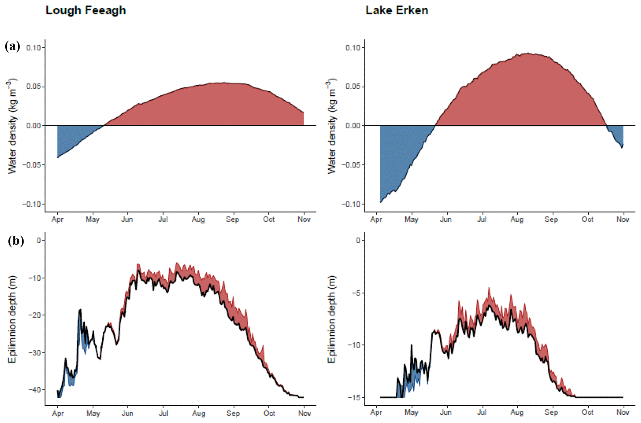
Figure 3Long-term mean for each Julian day of the difference in water density (kg m−3) induced by an increase of 1 ∘C in water temperature, relative to 0.1 kg m−3 (black line with the red shaded area demonstrating when the change induced by an increase of 1 ∘C change was greater than 0.1 kg m−3 and the blue shaded area for when it was less than 0.1 kg m−3) (a). The long-term mean for each Julian day of epilimnion depth calculated using a water temperature threshold of 1 ∘C (the black line) compared to a water density threshold of 0.1 kg m−3 (shaded area, with the red shaded areas demonstrating when water density estimates were shallower and the blue shaded area for when they were deeper) (b) for Lough Feeagh and Erken lake.
3.2 Comparison between water-density-based methods (M1–M4)
Inspection of water column profiles highlighted key differences in the performance of methods M1–M4 (Fig. 4). In a stratified profile, with a well-defined three-layered water column profile, there was often strong agreement on the epilimnion depth between all methods and thresholds (Fig. 4a). In contrast, when the measured temperature profile was more complex, i.e. at times when there was some stratification close to the surface or when a secondary pycnocline had developed close to the surface, there was less agreement on the estimates of the epilimnion depth between methods (Fig. 4b). For such profiles, estimates of the epilimnion depth calculated with the absolute difference from the surface method, M1, were typically staggered at linear intervals along the profile, depending on the exact threshold value. In contrast, the estimated epilimnion depth calculated using the gradient methods (M2–M4) had a tendency to cluster at discrete locations on the profile. Therefore, a small change in the threshold value induced either no difference at all in the epilimnion depth or at other times a very large difference. For profiles with low water column stability, there was particularly large differences in the estimated epilimnion depth calculated using different methods, reflecting differing underlying assumptions (Fig. 4c). For M3, for example, the epilimnion depth was defaulted to the deepest depth when the threshold value was not exceeded, as was also the case for methods M1 and M2. In contrast, however, in M4, near-isothermal profiles often met the “mixed.cutoff” filter condition (i.e. water column range > 1 ∘C), whilst still not having sufficient density gradients to meet the user threshold value. As a result, in M4, the epilimnion depth was defaulted to the pycnocline, which, given the small density gradients, was often found at a very shallow depth.
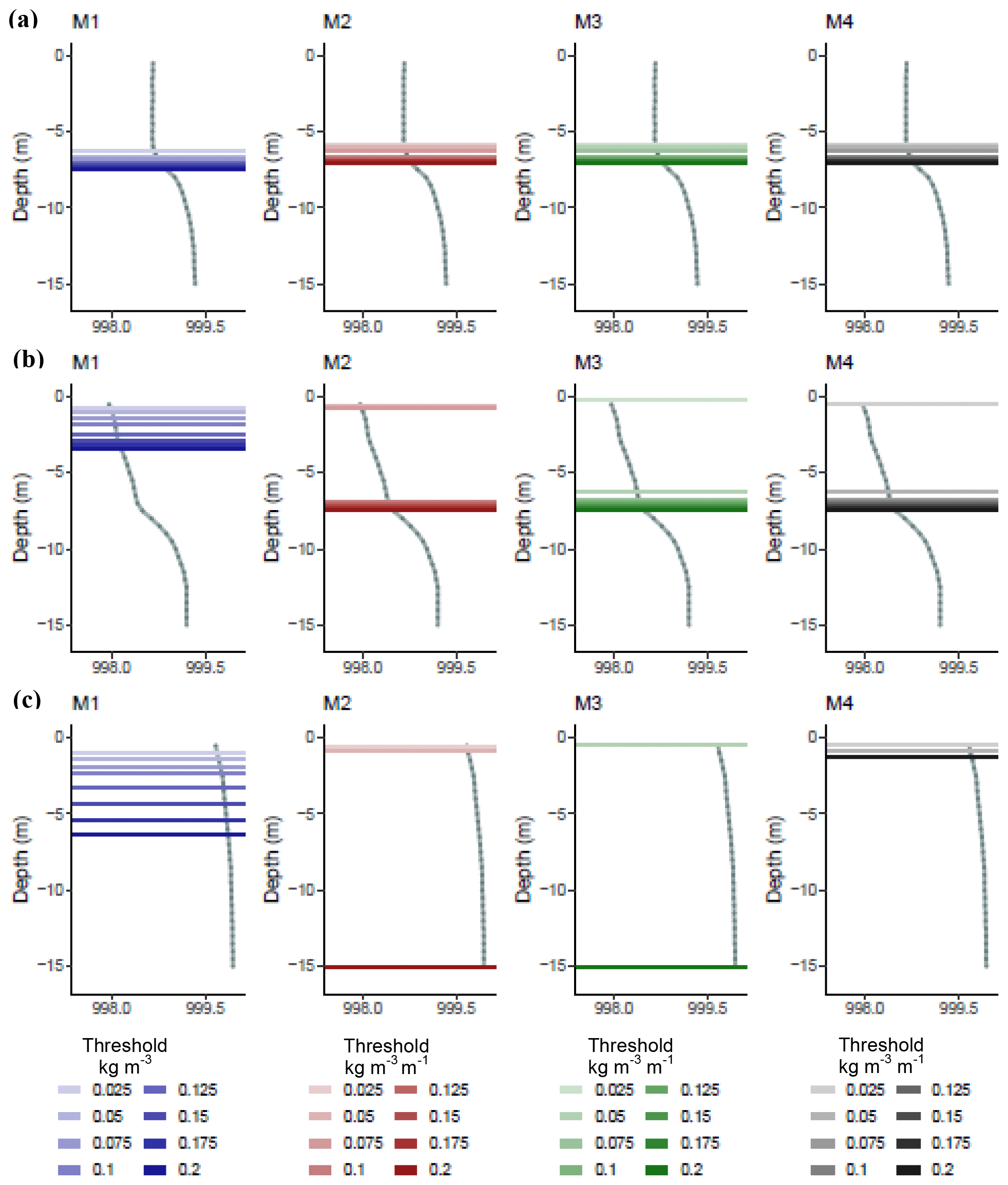
Figure 4An example of water column profiles with the epilimnion depth estimates superimposed (horizontal lines) for all profile-based epilimnion depth methods calculated using the full range of thresholds for each. The water columns can be categorised as a three-layered water column structure (a), an intensely stratified profile (b), and a near-isothermal profile (c), which are all from Erken lake only.
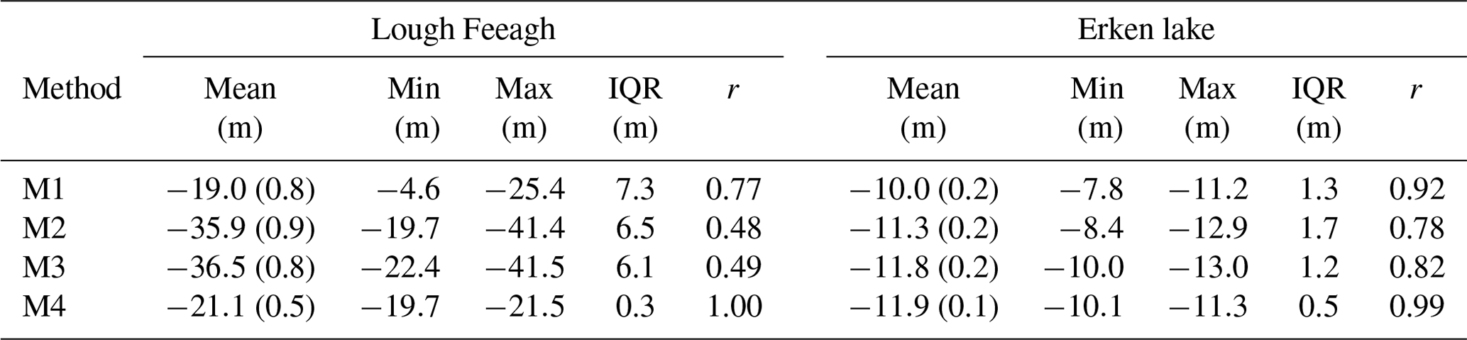
Table 2Summary of statistics for each method, showing the mean (m) and standard error of the mean in brackets, minimum (i.e. shallowest estimate) (m), maximum (i.e. deepest estimate) (m), interquartile range (IQR, m) of the April–October epilimnion depth estimates (summarised from the results shown in Fig. 6a), and the mean Pearson's correlation coefficient (r) for each method, representing the mean correlation for all possible combinations between threshold values for Lough Feeagh and Erken lake.
Time series results demonstrated the extent of the variability in epilimnion depth estimates between all methods and thresholds (Fig. 5). Considering that all the time series estimates for Lough Feeagh (left side) and Erken lake (right side) were presumed to estimate the same theoretical location, they would ideally all produce exactly the same temporal patterns. Instead, the differences were large enough to obscure the annual patterns and hinder the ability to compare between the two lakes. The overall mean epilimnion depth estimate using methods M1–M4 and all thresholds was −28.1 m (standard error SE = 0.6 m, interquartile range IQR = 19.0 m) for Lough Feeagh and −11.0 m (SE = 0.1 m, IQR = 2.3 m) for Erken lake. The overall variability between all estimates was particularly high for Lough Feeagh, where the April–October mean epilimnion depth ranged by 36.9 m (−4.6 to −41.5 m), while in Erken lake estimates ranged by 5.2 m (−7.8 to −13.0 m) (Fig. 6a).
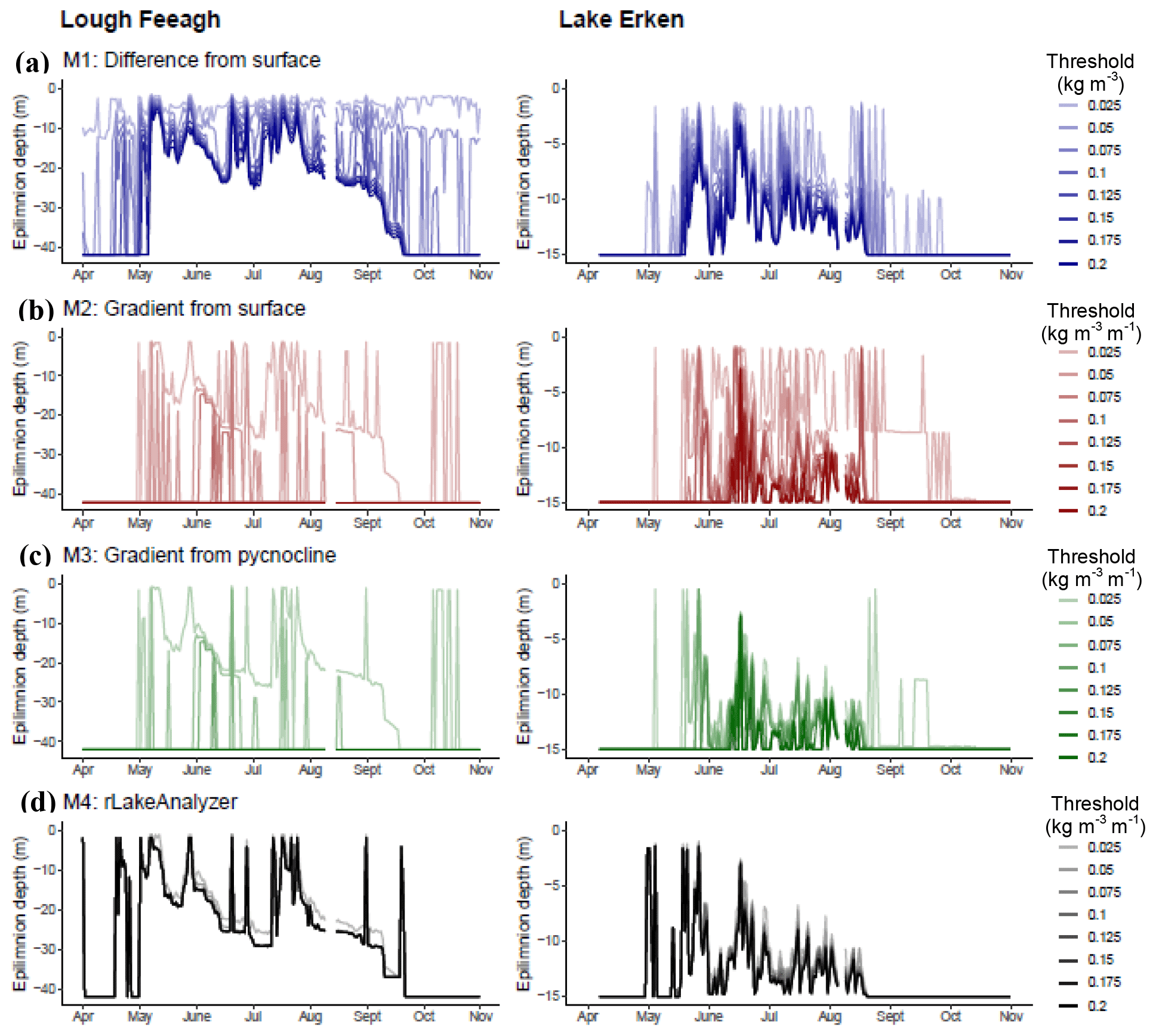
Figure 5Daily epilimnion depth estimates using measured data for 2017 from Lough Feeagh and Erken lake, showing estimates from all profile-based epilimnion depth methods, including M1, the absolute difference from the surface method (a); M2, the gradient from the surface method (b); M3, the gradient from the pycnocline method (c); and M4, the rLakeAnalyzer method (d), which are calculated using the full range of thresholds and for each lake.
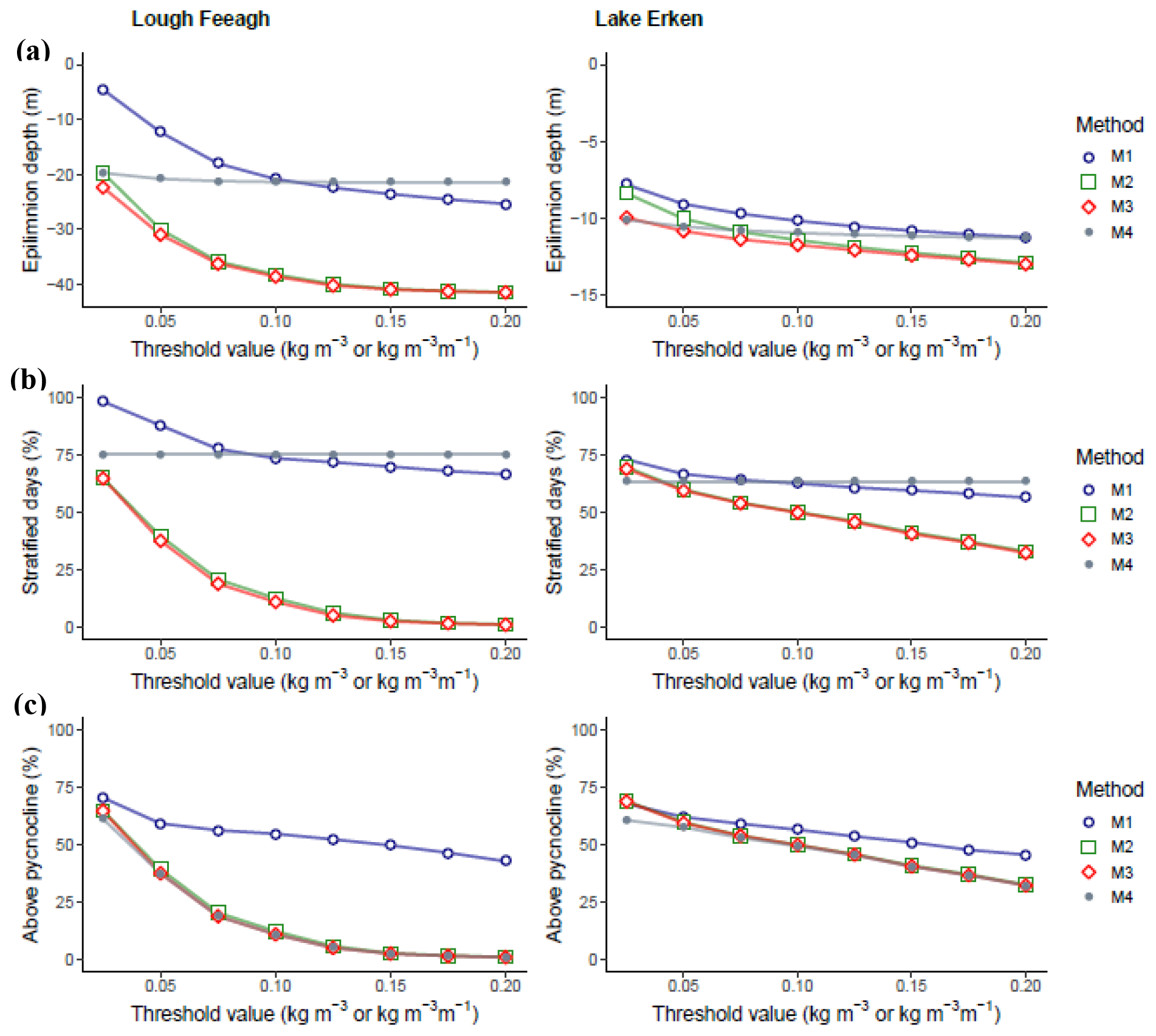
Figure 6Mean April–October epilimnion depth (m) (a); percentage of stratified days, defined as days when the epilimnion depth was identified as shallower than the lake maximum measured depth (%) (where a larger percentage value indicated a higher occurrence of days identified as stratified) (b); and percentage of days when the epilimnion depth was above the pycnocline, defined as the number of days when the epilimnion was identified at a depth shallower than the maximum density gradient (where a larger percentage value indicated a lower occurrence of days erroneously extending into the metalimnion) (c) for Lough Feeagh and Erken lake.
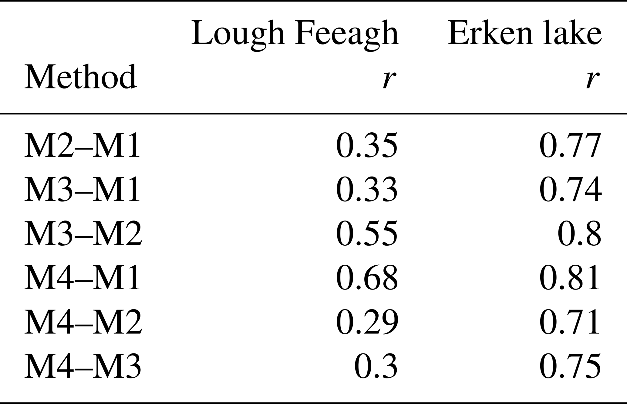
There were evident systematic differences between methods. In both lakes, the mean April–October epilimnion depth for each method was shallowest for M1 and was on average shallower by 17.0, 16.6, and 2.2 m compared with methods M2–M4 in Lough Feeagh and 1.2, 1.7, and 0.8 m in Erken lake (Table 2). The minimum (shallowest) estimates of the April–October mean for gradient methods (M2–M4) were comparable in magnitude to the maximum (deepest) estimate for the absolute difference from the surface method, M1. The mean Pearson's correlation coefficient between each pair of methods also demonstrated that certain method pairs had greater temporal agreement than other pairs (Table 3). The full correlation matrices are available in Table S2. Method pairs M3–M2 and M4–M1 had particularly high Pearson correlation coefficients for both lakes, suggesting these methods produced similar temporal trends. In Erken lake all method pairs had higher Pearson's correlation coefficients than Lough Feeagh.
Table 3Mean of all Pearson's correlation coefficients calculated for each pair of methods (e.g. for all threshold combinations between M1 and M2) for Lough Feeagh and Erken lake.
The selection of a threshold value proved to be very important in the estimation of the epilimnion depth. For all methods, smaller threshold values produced shallower estimates of the mean April–October epilimnion depth, while larger threshold values produced deeper estimates (Fig. 6a). Methods with a wide range between the shallowest (minimum) and deepest (maximum) estimate demonstrated high sensitivity to the threshold value (Table 2). For both lakes, the interquartile range in the mean April–October epilimnion depth estimates for each method was very high for M2, M1, and M3, indicating high threshold sensitivity in these methods. Method M4 had a substantially lower interquartile range than all other methods and a very high mean Pearson's correlation coefficient, indicating that both the mean value and the temporal pattern of the epilimnion depth were only weakly influenced by the threshold value. In both lakes, methods M2 and M1, where the epilimnion depth was defined from the surface downwards, had a higher interquartile range in estimates calculated with different threshold values compared to methods M3 and M4, where the epilimnion was defined from the pycnocline upwards. M1, however, had higher mean Pearson's correlation coefficient than M2 and M3, indicating that the temporal pattern of the epilimnion depth was less influenced by the threshold value. In general, the threshold sensitivity of each method reduced with increasing threshold size. That is, the changes in the epilimnion depth occurring between threshold values decreased with increasing threshold value (Fig. 6a). For example, for M2, the difference in the April–October mean epilimnion depth between the first two thresholds (0.025 and 0.05 kg m−3 m−1) was much greater than the difference between the last two thresholds (0.175 and 0.2 kg m−3 m−1) in both lakes.
The percentage of stratified days, defined as days when the epilimnion depth was identified as shallower than the deepest measured depth, demonstrated the extent to which different methods/thresholds influenced the stratified period (Fig. 6b). For M4, the percentage of stratified days remained static regardless of the threshold value, because the epilimnion depth was detected for all profiles where the water column temperature range was more than 1 ∘C, regardless of the threshold used. For all other methods, the number of stratified days decreased with increasing threshold value. For M1 the difference in stratified days between threshold values was small compared to both gradient methods M2 and M3, particularly in Lough Feeagh. For example, in Lough Feeagh, for M3, the number of stratified days calculated using a threshold value of 0.025 kg m−3 m−1 was 125, while for threshold values greater than 0.075 kg m−3 m−1, the mean number of stratified days per annum decreased to less than 38.
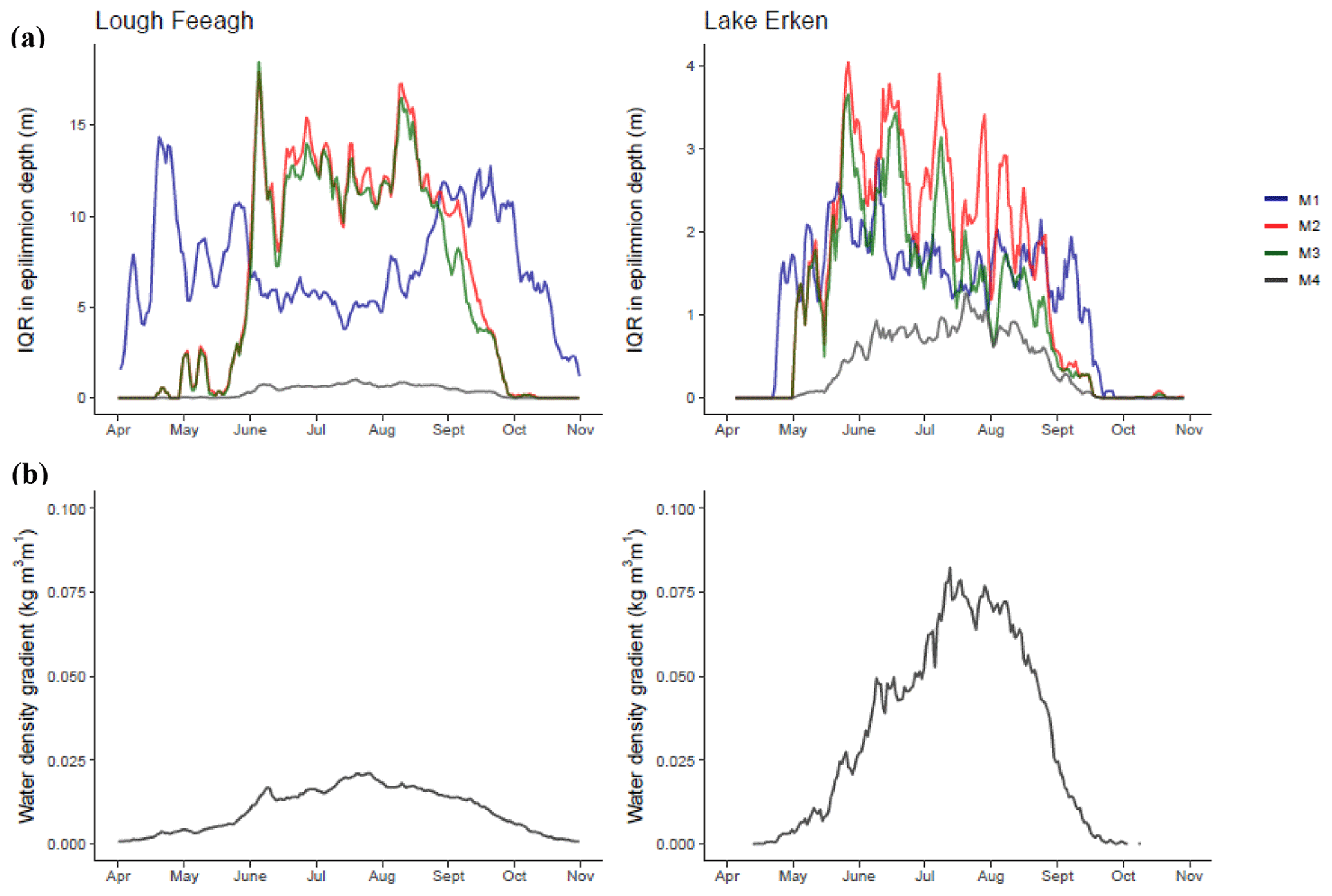
Figure 7Interquartile range between the shallowest and deepest estimate for each method calculated from long-term daily mean epilimnion depth estimates for each Julian day, when a wide range suggests high threshold sensitivity and a narrow range suggests low sensitivity (a); long-term daily mean water density gradient, calculated based on the surface and maximum measured depths (b) for Lough Feeagh and Erken lake.
The percentage of days when the epilimnion depth was located above the pycnocline, defined as days when the epilimnion depth was identified above the maximum density gradient, indicated that some methods may be less prone to erroneously estimating the epilimnion depth in the metalimnion compared with others (Fig. 6b). For both lakes, M1 had the highest number of days when the epilimnion depth was located above the pycnocline, suggesting that on average the method extended into the metalimnion less frequently than other methods. In Lough Feeagh, all gradient methods, M2–M4, had very high range occurring between the different threshold values. In Lough Feeagh, gradient methods calculated with a threshold value greater than 0.1 kg m−3 m−1 resulted in an average of 0 d when the epilimnion depth was located above the pycnocline.
3.3 Sensitivity of epilimnion depth to water column structure
For all methods, threshold sensitivity fluctuated seasonally, although it varied in a pattern (Fig. 7). Threshold sensitivity was shown by the interquartile range between the epilimnion depth estimates calculated for all threshold values. In Lough Feeagh, M1 had a smaller interquartile range in epilimnion depth estimates during the peak summer months of June, July, and August compared with months when the onset and overturn of stratification commonly occurred. During periods of transient stratification, the stability of the water column was often low, but frequent changes in the near-surface water density induced large difference between estimates calculated using small thresholds compared with large threshold values. In contrast, methods M2 and M3 had the highest interquartile range in estimates occurring during the peak summer months. Even during peak summer in Lough Feeagh, gradients in the water column were relatively small (Fig. 7b), which resulted in a very large differences between the smallest threshold values which found a near-surface epilimnion depth and the largest thresholds that often found no epilimnion depth at all and therefore defaulting to the deepest depth. In Erken lake, the water density gradients were typically much larger, and methods M1–M3 all peaked during May and June, when gradients in the water column were typically increasing but prone to fluctuations. Compared with all other methods, M4 produced a substantially lower interquartile range in the epilimnion depth throughout the year, since as long as the “mixed.cutoff” filter was met, the epilimnion depth was defaulted to the pycnocline if the threshold was not exceeded and thus largely reducing the ability for large differences to occur. The interquartile range in epilimnion depth estimates for M4 was highest during the peak summer months, which was when the epilimnion depth was typically shallowest and more frequently defined by the threshold value rather than defaulting to the pycnocline.
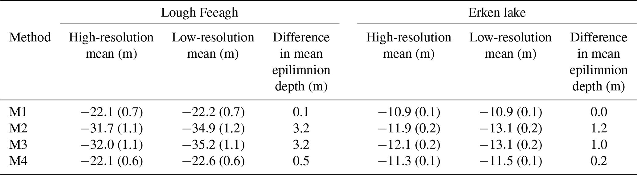
Table 4Mean April–October epilimnion depth estimates (m) derived using high-resolution and low-resolution modelled water temperature data, with standard error of the mean in brackets, and the difference calculated between the high-resolution and low-resolution estimates (m) for Lough Feeagh and Erken lake.
3.4 Sensitivity of epilimnion depth to vertical sensor resolution
The vertical resolution of water density data was found to have a systematic influence on the estimation of the epilimnion depth for all methods (Table 4). Overall, the modelled higher vertical resolution data resulted in shallower estimates of the epilimnion depth relative to the estimates made with the modelled low-resolution data. For Lough Feeagh, the results showed that the annual mean April–October epilimnion depth estimates using high-resolution data were 0.1, 3.2, 3.2, and 0.5 m shallower than those using low-resolution data for methods M1–M4, while in Erken lake they were 0.0, 1.2, 1.0, and 0.2 m shallower. Methods M1 and M4 had substantially smaller differences between high- and low-resolution estimates compared with M2 and M3. In particular, M1 had almost no difference between high- and low-resolution data, indicating that this method had very low sensitivity to the vertical sensor deployment.
3.5 Comparison with modelled turbulence method (M5)
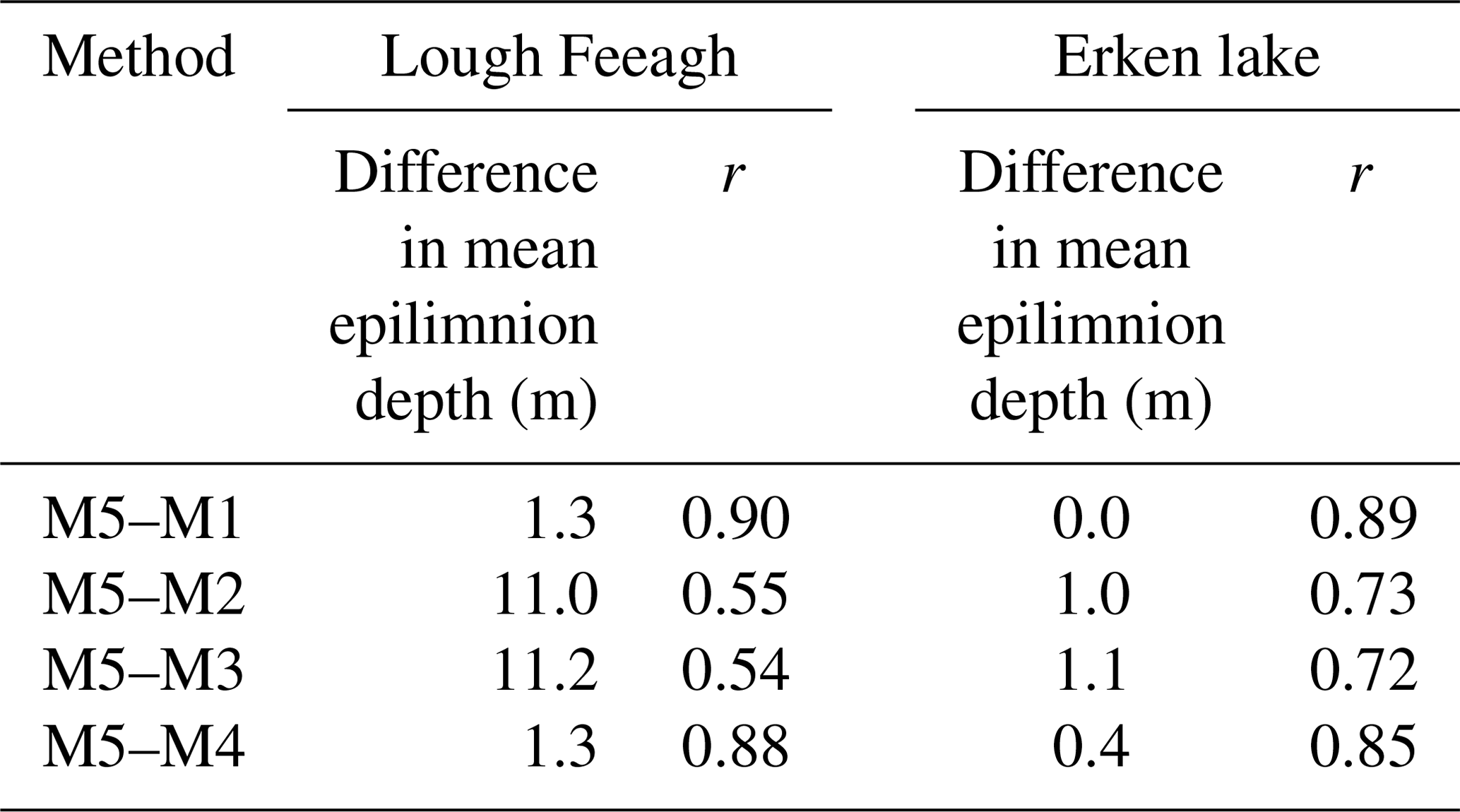
In general, the modelled turbulence method had very low sensitivity to the threshold value compared with the profile-based methods also calculated using modelled data. A time series comparison of all modelled results is available in Fig. S1 (in the Supplement). For both lakes, we found that the modelled turbulence method produced shallower estimates than modelled profile-based methods (Table 5). In Lough Feeagh, the mean April–October epilimnion depth estimate using the modelled turbulence method M5 was −20.8 m, which was 1.3, 11.0, 11.2, and 1.3 m shallower than methods M1–M4, while in Erken lake the M5 estimate was −11.0 m, which was 0.0, 1.0, 1.1, and 0.4 m shallower. In both lakes, M1 had the strongest agreement with M5, demonstrated by both the mean difference (1.3 m in Lough Feeagh and 0.0 m in Erken lake) and the highest Pearson's correlation coefficient in Lough Feeagh (r=0.90) and Erken lake (r=0.89). This was followed by M4, which also had strong agreement with M5. In contrast, M2 and M3 had much weaker agreement with M5, in terms of both the April–October epilimnion depth estimate and the Pearson's correlation coefficients.
Table 5Difference in mean April–October epilimnion depth estimates (m) between each profile-based method (M1–M4) calculated using lake modelled data and the modelled turbulence method (M5) and mean of all Pearson's correlation coefficients (r) calculated for each profile-based method and M5 (e.g. for all threshold combinations between M5 and M1) for Lough Feeagh and Erken lake. Positive differences indicate that the modelled turbulence method is shallower.
The concept of the epilimnion (and, more widely, the three-layered structure of a stratified lake) is fundamental in limnology. Yet, despite the ubiquity of the term, there is no objective or generic approach for defining the epilimnion, and a diverse number of approaches prevail in the literature. In a comprehensive analysis of high-frequency multi-year data from two lakes, this study has highlighted the extent to which common water-temperature-profile-based epilimnion depth estimates differ. The level of variability in epilimnion depth estimates calculated using common methods and threshold values was exceedingly high. This result calls into question the practice of arbitrary method selection and comparing findings between studies which use different methods or even just different thresholds. The magnitude of variability also casts ambiguity on the calculation of key biogeochemical and ecological processes in a lake that rest on the assumption that the layers of a lake are well defined, including calculations of metabolic rates and oxygen fluxes (e.g. Coloso et al., 2011; Foley et al., 2012; Obrador et al., 2014; Winslow et al., 2016).
In an idealised stratified profile, the epilimnion is portrayed as near uniform in water temperature or density and clearly delineated from a well-defined metalimnion. However, many measured profiles, at least within this study, did not conform to this idealised three-layered structure. Instead the thermal water column structure was often more complex, including multiple pycnoclines, near-surface micro-stratification layers, and blurred boundaries between the epilimnion and metalimnion. One approach to this issue is to filter out appropriate water column profiles or apply functions that coerce the profile into the expected structure (Read et al., 2011; Pujoni et al., 2019; Gray et al., 2020). However, our analysis of temporally high-resolution time series data emphasised that rather than jumping from states, such as stratified or isothermal, changes in the water column occurred over an evolving continuum and often fluctuated between states. Similarly, the distinction between additional layers, such as the primary or secondary pycnocline, is fraught with the same issues of arbitrariness as discussed (Read et al., 2011). This study demonstrates that when epilimnion depth estimation methods, which are theorised for a three-layered water column, are applied to nonconforming water columns, they diverge widely on the location of the epilimnion depth, and at times may not even be underpinned by the same theoretical assumptions. Since none of these methods can be considered the true definition of the epilimnion depth, it is necessary to understand the degree to which methods differ. Improved understanding of their systematic differences will facilitate the use of methods that appropriately capture different processes, such as air–water exchanges, thermocline entrainment, or the suspension of materials. Due to the realised complexities of observed and aggregated profile data, we may benefit from new approaches to water column discretisation that consider the vast proportion of profiles which do not conform neatly to the three-layered paradigm.
A large systematic difference was found between water temperature and water density. Due to the non-linear relationship between water density and temperature, the use of water temperature was equivalent to using different density threshold values throughout the year, resulting in a distinct shift in the stratification period. Although water density gradients are driven by temperature changes in lakes and are also calculated from water temperature estimates, water density directly influences mixing processes and is therefore recommended for estimating the epilimnion depth (Read et al., 2011; Gray et al., 2020). The implications of using a water-temperature-based method may be particularly enhanced in northern temperate lakes due to the large annual water temperature ranges (Maberly et al., 2020). Pronounced differences in the estimation of the epilimnion depth were also found within estimates derived using the same water density input data. Typically, for the range of common thresholds used in this study, the absolute difference from the surface method, M1, produced shallower estimates relative to gradient-based methods. In addition, the difference between these methods was particularly large when the vertical resolution of the data was low. This suggests that studies using gradient-based methods, particularly those using coarse vertical data, may have a deep bias relative to those using an absolute method and, consequently, were more prone to erroneously extending into the metalimnion. In addition, as may be expected, the use of larger threshold values also produced systematically deeper estimates of the epilimnion depth. Surprisingly, however, the magnitudes of these differences were on par with those occurring between methods. The implications of a shallow or deep bias may be far reaching, particularly given that various biological and ecological metrics have already been found to be highly sensitive to changes in the epilimnion depth (Coloso et al., 2011; Gray et al., 2020). For example, a deeper estimate of the epilimnion depth would systematically lead to a larger ratio between the epilimnion and euphotic depth compared with a shallower estimate, which if used to understand the development of a phytoplankton bloom, could lead to contradictory results (Huisman et al., 1999). Alternatively, water-temperature-based estimates typically resulted in earlier stratification, which could indicate a longer duration of phytoplankton in a shallower epilimnion. The implications of a seasonal or deep/shallow biases may be even more important for computing fluxes (e.g. oxygen or nutrients) between the epilimnion and the metalimnion, since both terms are influenced by the epilimnion depth (Giling et al., 2017; Gray et al., 2020).
An important difference was also found between methods detecting the layer that is isothermal relative to the surface and methods detecting the point that is isothermal relative to the steep gradients of the metalimnion, which has not been well considered in the literature. M1 and M2, defined from the surface downwards, were more prone to the detection of a shallow secondary pycnocline compared with M3 and M4. Instead, M3 and M4, defined from the pycnocline upwards, prioritised the relative difference between the metalimnion and the surface. From a theoretical point of view, processes related to the air–water interface could be better suited to methods identifying the isothermal layer, while processes related to the entrainment of deep water into the epilimnion are more suited to top of the metalimnion methods.
The selection of an epilimnion method also had surprisingly large consequences for understanding the stratification period, which is widely used for quantifying the impact of climate change on lakes (Livingstone, 2003; Butcher et al., 2015; Ayala et al., 2020). Notably, the mean epilimnion depth and number of stratified days calculated using M4 depended very little on the threshold value selected. Instead, the selection of the filter (defaulted to a water column range of >1 ∘C), which was unique to this method, determined the number of stratified days and largely influenced the other bulk statistics. This also resulted in the epilimnion being identified even when the threshold was not exceeded, which in some instances could have the effect of muting relative temporal changes in the epilimnion depth. In contrast, for the other methods, the threshold was used to determine whether the water column was considered to be stratified; therefore, the stratification period was highly sensitive to the threshold value, similarly to the other bulk statistics. Ultimately, these results suggest that the stratification period calculated in different studies or for different regions cannot be compared unless identical definitions are used. The method most appropriate for identifying the stratified period has been considered in other studies (Woolway et al., 2014; Engelhardt and Kirillin, 2014; however, our results offer some additional insights. The results suggest that the use of water density metrics, such as epilimnion depth estimates, in combination with traditional water-temperature-based definitions of stratification, is incompatible, given the non-linear relationship between temperature and density. In addition, estimations of the epilimnion depth (and the variability among definitions) may be particularly relevant for understanding the stratified period, since it is often assumed that the onset of stratification marks the decoupling of the epilimnion from the deeper layers, determining the duration of nutrient limitations in the epilimnion and oxygen limitations in the hypolimnion (MacIntyre, 1993; Foley et al., 2012; Schwefel et al., 2016).
Regardless of the method selected, however, all water temperature- or density-based methods are limited in their ability to indicate actual mixing processes. Our results using the lake modelled turbulence data demonstrated that even in a modelled environment, epilimnion depth estimates were inconsistent between the different methods and threshold values studied and that turbulence-based methods generally resulted in a shallower epilimnion depth estimate. These findings highlight the important but subtle difference between the layer detected by water density profiles (i.e. has been recently well mixed and therefore has little resistance to further mixing due to the lack of density gradients) and the layer that is actively mixing, determined only through directly measured turbulence (Gray et al., 2020). Similarly, micro-profiling studies have shown that the actively mixing layer can be substantially shallower than the layer determined through water temperature profile data (McIntyre, 1993; Tedford et al., 2014). Micro-profile studies also demonstrate that within seemingly uniform layers there are micro-stratification layers, delineated by temperature differences as small as 0.02 ∘C (Imberger, 1985; Shay and Gregg, 1986; MacIntyre, 1993; Jonas et al., 2003), which can be sufficient to isolate intermediate layers from atmospheric wind shear and cooling (Pernica et al., 2014). Although our results are not directly indicative of measured data, they demonstrate how even turbulence-based methods are inherently arbitrary, as there is no objective threshold value (Monismith and Macintyre, 2009). Many of the ecological applications of the epilimnion depth have the underlying assumption that enough mixing is occurring in the epilimnion to keep the relevant organisms or particles suspended within the layer. However, whether mixing is actually occurring and to what extent are not directly described by epilimnion depth estimations derived using water temperature or density profile data; in fact, previous studies have found water density estimates of the epilimnion depth to be relatively poor indicators for the homogeneity of other ecological variables (Gray et al., 2020).
The selection of a suitable threshold value is far more important than previously attributed in limnology. In general, a suitable threshold is any value that can be reasonably considered homogenous while also within the limit of sensor detection (De Boyer et al., 2004). However, all the threshold values used in this study met these criteria yet produced fundamentally different epilimnion depth estimations and temporal patterns. Although it may be unreasonable to suggest a “universal” threshold value, a given study may find a threshold that is less problematic than other values. In general, we found that the sensitivity of the epilimnion depth to the threshold value decreased with the increasing size of the threshold. That is, for small thresholds the impact of changing the threshold value was greater than larger thresholds for the same incremental change. This may suggest that for studies using smaller threshold values, the results are more threshold dependent than those using large threshold values. However, larger threshold values had a greater frequency of the epilimnion depth estimates being below the maximum density gradient, suggesting that larger threshold values tend to extend into the stable depths of the metalimnion more regularly and hence somewhat explaining the lower threshold sensitivity. The trade-off between threshold sensitivity and encroachment into the metalimnion points towards a mid-range threshold, such as 0.1 kg m−3 or 0.1 kg m−3 m−1, as potentially being more reliable than large or small thresholds.
One of the main goals behind the global collection of high-frequency data in lakes is to understand how physical processes vary between lakes, which indicates how different lakes may respond to changing climatic conditions (Weathers et al., 2013; Kraemer et al., 2015; Woolway and Merchant, 2019). In order to understand this, we require methods that perform consistently between lakes and over longitudinal scales. The differences between the two lakes studied, in particular variability in water column structure, the strength of density gradients, and the vertical resolution of sensor deployment influenced the level of agreement between epilimnion depth methods. Overall, Erken lake had much greater agreement among methods than Lough Feeagh. In particular, we found this to be related to the difference in vertical resolution of the measured data between sites. Of all the methods considered in this study, our results suggest that the absolute difference from the surface method, M1, might be more useful as a “generic” method, due in particular to the very low sensitivity to the vertical sensor resolution compared with all other gradient-based methods. This finding is in agreement with previous oceanography studies that have similarly found gradient methods to be highly sensitive to vertical resolution (e.g. Lorbacher et al., 2006; Thomson and Fine, 2003). In addition, however, the performance and threshold sensitivity of all methods also fluctuated temporally as influenced by changes in the water column structure. Assessment of the uncertainty associated with epilimnion depth estimates may be useful, particularly for studies comparing the epilimnion depth between periods of time that vary in stratification intensity.
Although long-term epilimnion depth trends are only rarely reported directly (e.g. Hondzo and Stefan, 1993; Fee et al., 1996; Sahoo et al., 2013), they are embedded in our understanding of many climate-related variables. For example, the epilimnion depth plays a key role in modulating the effects of eutrophication, browning, and climate change on lake water surface and epilimnetic temperatures (Persson and Jones, 2008; Flaim et al., 2016; Strock et al., 2017; Bartosiewicz et al., 2019). As such, changes in the epilimnion depth may enhance or mute the effect of increasing incoming heat on water surface temperatures and therefore may be particularly important in explaining temporal and spatial anomalies in surface temperature trends. Given the results of this study, it may be that long-term trends calculated using different metrics relate to fundamentally different parts of the water column that may be undergoing different changes due to climate change. Therefore, the strength and even the direction of long-term trends in the epilimnion may be highly dependent on the definition used (Yang and Wang, 2009; Somavilla et al., 2017).
This study has demonstrated that different definitions of the epilimnion depth lead to different locations of the epilimnion depth in the water column and produce very different and contradictory temporal patterns. These results have wide-reaching relevance in limnology, including studies interested in metabolism, eutrophication, and hypolimnetic anoxia. The sensitivity of epilimnion depth methods to temporal and spatial characteristics, such as morphology, water column structure, and vertical resolution of data measurements may also pose challenges for studies interested in long-term trends or global lake comparison studies. While there is no prescribed rationale for selecting a particular method, the M1 method, defined as the shallowest depth where the density was 0.1 kg m−3 more than the surface density, was shown to be particularly insensitive to the vertical sensor resolution of water temperature data, while the temporal pattern was relatively robust to changes in the threshold value. Therefore, the M1 method may be particularly useful as a generic method.
The analysis codes and output data are stored in HydroShare http://www.hydroshare.org/resource/26dbc260405b4bb9b3ac16ec55432684 (last access: 19 November 2020) (Wilson et al., 2020). Source code of the model GOTM is freely available online at https://gotm.net/ (last access: 25 June 2020 (GOTM, 2020). The data used in this study from Lough Feeagh are available online at https://doi.org/10.20393/6C4760C2-7392-4347-8555-28BA0DAD0297 (de Eyto et al., 2020).
The supplement related to this article is available online at: https://doi.org/10.5194/hess-24-5559-2020-supplement.
The original study concept was devised by IDJ, MEP, EJ, and DP. Funding was acquired by EJ, DP, IDJ, HPG, EdE and RIW. EJ and AR were the project administrators. Data were curated by EdE and DP. The investigation was carried out by HLW, AIA, IJ, EJ, DP, HPG and RIW. The formal analysis was done by HLW and AIA. HLW was supervised by EJ, IDJ, HPG, DP and AR. The draft was written by HLW, and all authors contributed to the review and editing process.
The authors declare that they have no conflict of interest.
This research was carried out as part of the MANTEL Innovative Training Network, which has received funding from the European Union's Horizon 2020 research and innovation programme under the Marie Skłodowska-Curie grant agreement no. 722518 (H2020-MSCA-ITN-2016). In addition, R. Iestyn Woolway received funding from the European Union's Horizon 2020 research and innovation programme under the Marie Skłodowska-Curie grant agreement no. 791812. The long-term monitoring program of Lough Feeagh is enabled by the field staff of the Marine Institute (Ireland), and we gratefully acknowledge their support. The monitoring program at Erken lake received financial support from the Swedish Infrastructure for Ecosystem Science (SITES).
This research has been supported by the European Union's Horizon 2020 Marie Skłodowska-Curie grant no. 722518 (H2020-MSCA-ITN-2016) and grant no. 791812 (R. Iestyn Woolway).
This paper was edited by Anas Ghadouani and reviewed by two anonymous referees.
Andersen, M. R., Sand-Jensen, K., Woolway, R. I., and Jones, I. D.: Profound daily vertical stratification and mixing in a small, shallow, wind-exposed lake with submerged macrophytes, Aquat. Sci., 79, 395–406, https://doi.org/10.1007/s00027-016-0505-0, 2017.
Ayala, A. I., Moras, S., and Pierson, D. C.: Simulations of future changes in thermal structure of Lake Erken: proof of concept for ISIMIP2b lake sector local simulation strategy, Hydrol. Earth Syst. Sci., 24, 3311–3330, https://doi.org/10.5194/hess-24-3311-2020, 2020.
Bartosiewicz, M., Przytulska, A., Lapierre, J. F., Laurion, I., Lehmann, M. F., and Maranger, R.: Hot tops, cold bottoms: Synergistic climate warming and shielding effects increase carbon burial in lakes, Limnol. Oceanogr. Lett., 4, 132–144, https://doi.org/10.1002/lol2.10117, 2019.
Berger, S. A., Diehl, S., Kunz, T. J., Albrecht, D., Oucible, A. M., and Ritzer, S.: Light supply, plankton biomass, and seston stoichiometry in a gradient of lake mixing depths, Limnol. Oceanogr., 51, 1898–1905, https://doi.org/10.4319/lo.2006.51.4.1898, 2006.
Bouffard, D. and Wüest, A.: Mixing in stratified lakes and reservoirs, in: Mixing and dispersion in flows Dominated by Rotation and Buoyancy, Springer, Cham, 61–88, https://doi.org/10.1007/978-3-319-66887-1_3, 2018.
Brainerd, K. E. and Gregg, M. C.: Surface mixed and mixing layer depths, Oceanogr. Literat. Rev., 4, 1521–1544, https://doi.org/10.1016/0967-0637(95)00068-H, 1996.
Burchard, H., Bolding, K., and Villarreal, M. R.: GOTM. a General Ocean Turbulence Model, Theory, implementation and test cases, Technical Report EUR 18745 EN, European Commission, 1999.
Butcher, J. B., Nover, D., Johnson, T. E., and Clark, C. M.: Sensitivity of lake thermal and mixing dynamics to climate change, Climatic Change, 129, 295–305, https://doi.org/10.1029/2010WR009104, 2015.
Calderó-Pascual, M., de Eyto, E., Jennings, E, Dillane, M., Andersen, M., Kelly, S., Wilson, H., and McCarthy, V.: Effects of consecutive extreme weather events on a temperate dystrophic lake: A detailed insight into physical, chemical and biological responses, Water, 12, 1411, https://doi.org/10.3390/w12051411, 2020.
Coloso, J. J., Cole, J. J., and Pace, M. L.: Short-term variation in thermal stratification complicates estimation of lake metabolism, Aquat. Sci., 73, 305–315, https://doi.org/10.1007/s00027-010-0177-0, 2011.
de Boyer Montégut, C., Madec, G., Fischer, A. S., Lazar, A., and Iudicone, D.: Mixed layer depth over the global ocean: An examination of profile data and a profile-based climatology, J. Geophys. Res.-Oceans, 109, C12003, https://doi.org/10.1029/2004JC002378, 2004.
de Eyto, E., Jennings, E., Ryder, E., Sparber, K., Dillane, M., Dalton, C., and Poole, R.: Response of a humic lake ecosystem to an extreme precipitation event: physical, chemical, and biological implications, Inland Waters, 6, 483–498, https://doi.org/10.1080/IW-6.4.875, 2016.
de Eyto, E., Dillane, M., Moore, T., Wilson, H., Cooney, J., Hughes, P., Murphy, M., Nixon, P., Sweeney, D., and Poole, R.: Lough Feeagh water temperature profiles, Marine Institute, Ireland, https://doi.org/10.20393/6C4760C2-7392-4347-8555-28BA0DAD0297, 2020.
Diehl, S., Berger, S., Ptacnik, R., and Wild, A.: Phytoplankton, light, and nutrients in a gradient of mixing depths: field experiments, Ecology, 83, 399–411, https://doi.org/10.1890/0012-9658(2002)083[0399:PLANIA]2.0.CO;2, 2002.
Dong, F., Mi, C., Hupfer, M., Lindenschmidt, K. E., Peng, W., Liu, X., and Rinke, K.: Assessing vertical diffusion in a stratified lake using a three dimensional hydrodynamic model, Hydrol. Process., 34, 1131–1143, https://doi.org/10.1002/hyp.13653, 2019.
Engelhardt, C. and Kirillin, G.: Criteria for the onset and breakup of summer lake stratification based on routine temperature measurements, Fundament. Appl. Limnol./Arch. Hydrobiol., 184, 183–194, https://doi.org/10.1127/1863-9135/2014/0582, 2014.
Fee, E. J., Hecky, R. E., Kasian, S. E. M., and Cruikshank, D. R.: Effects of lake size, water clarity, and climatic variability on mixing depths in Canadian Shield lakes, Limnol. Oceanogr., 41, 912–920, https://doi.org/10.4319/lo.1996.41.5.0912, 1996.
Flaim, G., Eccel, E., Zeileis, A., Toller, G., Cerasino, L., and Obertegger, U.: Effects of re-oligotrophication and climate change on lake thermal structure, Freshwater Biol., 61, 1802–1814, https://doi.org/10.1111/fwb.12819, 2016.
Foley, B., Jones, I. D., Maberly, S. C., and Rippey, B.: Long-term changes in oxygen depletion in a small temperate lake: effects of climate change and eutrophication, Freshwater Biol., 57, 278–289, https://doi.org/10.1111/j.1365-2427.2011.02662.x, 2012.
Giling, D. P., Staehr, P. A., Grossart, H. P., Andersen, M. R., Boehrer, B., Escot, C., Evrendilek, F., Gómez-Gener, L., Honti, M., Jones, I. D., and Karakaya, N.: Delving deeper: Metabolic processes in the metalimnion of stratified lakes, Limnol. Oceanogr., 62, 1288–1306, https://doi.org/10.1002/lno.10504, 2017.
GOTM: Software, available at: https://gotm.net/portfolio/software/, last access: 25 June 2020.
Goudsmit, G.H., Burchard, H., Peeters, F., and Wüest, A.: Application of k-ϵ turbulence models to enclosed basins: The role of internal seiches, J. Geophys. Res.-Oceans, 107, 3230, https://doi.org/10.1029/2001JC000954, 2002.
Gray, E., Mackay, E. B., Elliott, J. A., Folkard, A. M., and Jones, I. D.: Wide-spread inconsistency in estimation of lake mixed depth impacts interpretation of limnological processes, Water Res., 168, 115136, https://doi.org/10.1016/j.watres.2019.115136, 2020.
Hondzo, M. and Stefan, H. G.: Regional water temperature characteristics of lakes subjected to climate change, Climatic Change, 24, 187–211, https://doi.org/10.1007/BF01091829, 1993.
Huisman, J. E. F., van Oostveen, P., and Weissing, F. J.: Critical depth and critical turbulence: two different mechanisms for the development of phytoplankton blooms, Limnol. Oceanogr, 44, 1781–1787, https://doi.org/10.4319/lo.1999.44.7.1781, 1999.
Imberger, J.: The diurnal mixed layer, Limnol. Oceanogr., 30, 737–770, https://doi.org/10.4319/lo.1985.30.4.0737, 1985.
Jassby, A. and Powell, T.: Vertical patterns of eddy diffusion during stratification in Castle Lake, California, Limnol. Oceanogr., 20, 530–543, https://doi.org/10.4319/lo.1975.20.4.0530, 1975.
Jennings, E., Jones, S., Arvola, L., Staehr, P. A., Gaiser, E., Jones, I. D., Weathers, K. C., Weyhenmeyer, G. A., Chiu, C. Y., and De Eyto, E.: Effects of weather-related episodic events in lakes: an analysis based on high-frequency data, Freshwater Biol., 57, 589–601, https://doi.org/10.1111/j.1365-2427.2011.02729.x, 2012.
Jennings, E., de Eyto, E., Laas, A., Pierson, D., Mircheva, G., Naumoski, A., Clarke, A., Healy, M., Šumberová, K., and Langenhaun, D.: The NETLAKE Metadatabase – A Tool to Support Automatic Monitoring on Lakes in Europe and Beyond, Limnol. Oceanogr. Bull., 26, 95–100, https://doi.org/10.1002/lob.10210, 2017.
Jonas, T., Stips, A., Eugster, W., and Wüest, A.: Observations of a quasi shear-free lacustrine convective boundary layer: Stratification and its implications on turbulence, J. Geophys. Res.-Oceans, 108, 3328, https://doi.org/10.1029/2002JC001440, 2003.
Kara, A. B., Rochford, P. A., and Hurlburt, H. E.: Mixed layer depth variability over the global ocean, J. Geophys. Res.-Oceans, 108, 3079, https://doi.org/10.1029/2000JC000736, 2003.
Kraemer, B. M.: Rethinking discretization to advance limnology amid the ongoing information explosion, Water Res., 178, 115801, https://doi.org/10.1016/j.watres.2020.115801, 2020.
Kraemer, B. M., Anneville, O., Chandra, S., Dix, M., Kuusisto, E., Livingstone, D. M., Rimmer, A., Schladow, S. G., Silow, E., Sitoki, L. M., and Tamatamah, R.: Morphometry and average temperature affect lake stratification responses to climate change, Geophys. Res. Lett., 42, 4981–4988, https://doi.org/10.1002/2015GL064097, 2015.
Lamont, G., Laval, B., Pawlowicz, R., Pieters, R., and Lawrence, G. A.: Physical mechanisms leading to upwelling of anoxic bottom water in Nitinat Lake, in: 17th ASCE Engineering Mechanisms Conference, 13–16 June 2004, University of Delaware, Newark, USA, 2004.
Livingstone, D. M.: Impact of secular climate change on the thermal structure of a large temperate central European lake, Climatic Change, 57, 205–225, https://doi.org/10.1023/A:1022119503144, 2003.
Lorbacher, K., Dommenget, D., Niiler, P. P., and Köhl, A.: Ocean mixed layer depth: A subsurface proxy of ocean atmosphere variability, J. Geophys. Res.-Oceans, 111, C07010, https://doi.org/10.1029/2003JC002157, 2006.
Maberly, S. C., O'Donnell, R. A., Woolway, R. I., Cutler, M. E., Gong, M., Jones, I. D., Merchant, C. J., Miller, C. A., Politi, E., Scott, E. M., and Thackeray, S. J.: Global lake thermal regions shift under climate change, Nat. Commun., 11, 1–9, https://doi.org/10.1038/s41467-020-15108-z, 2020.
MacIntyre, S.: Vertical mixing in a shallow, eutrophic lake: Possible consequences for the light climate of phytoplankton, Limnol. Oceanogr., 38, 798–817, https://doi.org/10.4319/lo.1993.38.4.0798, 1993.
MacIntyre, S. and Melack, J. M.: Mixing Dynamics in Lakes Across Climatic Zones, in: Encyclopedia of inland waters, edited by: Linkens, G. E., Academic Press, Oxford, 603–612, https://doi.org/10.1016/B978-012370626-3.00040-5, 2009.
Marcé, R., George, G., Buscarinu, P., Deidda, M., Dunalska, J., de Eyto, E., Flaim, G., Grossart, H. P., Istvanovics, V., Lenhardt, M., and Moreno-Ostos, E.: Automatic high frequency monitoring for improved lake and reservoir management, Environ. Sci. Technol., 50, 10780–10794, https://doi.org/10.1021/acs.est.6b01604, 2016.
Martin, J. and McCutcheon, M.: Hydrodynamics and Transport for Water Quality Modeling, Lewis Publishers, New York, USA, 1999.
Monismith, S. G. and MacIntyre, S.: The surface mixed layer in lakes and reservoirs, in: Encyclopedia of inland waters, edited by: Linkens, G. E., Academic Press, Oxford, 636–650, https://doi.org/10.1016/B978-012370626-3.00078-8, 2009.
Moras, S., Ayala, A. I., and Pierson, D. C.: Historical modelling of changes in Lake Erken thermal conditions, Hydrol. Earth Syst. Sci., 23, 5001–5016, https://doi.org/10.5194/hess-23-5001-2019, 2019.
Nash, J. E. and Sutcliffe, J. V.: River flow forecasting through conceptual models part I – A discussion of principles, J. Hydrol., 10, 282–290, https://doi.org/10.1016/0022-1694(70)90255-6, 1970.
Obrador, B., Staehr, P. A., and Christensen, J. P.: Vertical patterns of metabolism in three contrasting stratified lakes, Limnol. Oceanogr., 59, 1228–1240, https://doi.org/10.4319/lo.2014.59.4.1228, 2014.
Pernica, P., Wells, M. G., and MacIntyre, S.: Persistent weak thermal stratification inhibits mixing in the epilimnion of north-temperate Lake Opeongo, Canada, Aquat. Sci., 76, 187–201, https://doi.org/10.1007/s00027-013-0328-1, 2014.
Persson, I. and Jones, I. D.: The effect of water colour on lake hydrodynamics: A modelling study, Freshwater Biol., 53, 2345–2355, https://doi.org/10.1111/j.1365-2427.2008.02049.x, 2008.
Pierson, D. C., Weyhenmeyer, G. A., Arvola, L., Benson, B., Blenckner, T., Kratz, T., Livingstone, D. M., Markensten, H., Marzec, G., Pettersson, K., and Weathers, K.: An automated method to monitor lake ice phenology, Limnol. Oceanogr.: Meth., 9, 74–83, https://doi.org/10.4319/lom.2010.9.0074, 2011.
Pujoni, D. G., Brighenti, L. S., Bezerra-Neto, J. F., Barbosa, F. A., Assunção, R. M., and Maia-Barbosa, P. M.: Modeling vertical gradients in water columns: A parametric autoregressive approach, Limnol. Oceanogr.: Meth., 17, 320–329, https://doi.org/10.1002/lom3.10316, 2019.
Read, J. S., Hamilton, D. P., Jones, I. D., Muraoka, K., Winslow, L. A., Kroiss, R., Wu, C. H., and Gaiser, E.: Derivation of lake mixing and stratification indices from high-resolution lake buoy data, Environ. Model. Softw., 26, 1325–1336, https://doi.org/10.1016/j.envsoft.2011.05.006, 2011.
Rivetti, I., Boero, F., Fraschetti, S., Zambianchi, E., and Lionello, P.: Anomalies of the upper water column in the Mediterranean Sea, Global Planet. Change, 151, 68–79, https://doi.org/10.1016/j.gloplacha.2016.03.001, 2017.
Sachse, R., Petzoldt, T., Blumstock, M., Moreira Martinez, S., Pätzig, M., Rücker, J., Janse, J., Mooij, W. M., and Hilt, S.: 485 Extending one-dimensional models for deep lakes to simulate the impact of submerged macrophytes on water quality, Environ. Model. Softw., 61, 410–423, https://doi.org/10.1016/j.envsoft.2014.05.023, 2014.
Sahoo, G. B., Schladow, S. G., Reuter, J. E., Coats, R., Dettinger, M., Riverson, J., Wolfe, B., and Costa-Cabral, M.: The response of Lake Tahoe to climate change, Climatic Change, 116, 71–95, https://doi.org/10.1007/s10584-012-0600-8, 2013.
Schwefel, R., Gaudard, A., Wüest, A., and Bouffard, D.: Effects of climate change on deepwater oxygen and winter mixing in a deep lake (Lake Geneva): Comparing observational findings and modeling, Water Resour. Res., 52, 8811–8826, https://doi.org/10.1002/2016WR019194, 2016.
Shay, T. J. and Gregg, M. C.: Convectively driven turbulent mixing in the upper ocean, J. Phys. Oceanogr., 16, 1777–1798, https://doi.org/10.1175/1520-0485(1986)016<1777:CDTMIT>2.0.CO;2, 1986.
Somavilla, R., González-Pola, C., and Fernández-Diaz, J.: The warmer the ocean surface, the shallower the mixed layer. How much of this is true?, J. Geophys. Res.-Oceans, 122, 7698–7716, https://doi.org/10.1002/2017JC013125, 2017.
Strock, K. E., Theodore, N., Gawley, W. G., Ellsworth, A. C., and Saros, J. E.: Increasing dissolved organic carbon concentrations in northern boreal lakes: Implications for lake water transparency and thermal structure, J. Geophys. Res.-Biogeo., 122, 1022–1035, https://doi.org/10.1002/2017JG003767, 2017.
Tedford, E. W., MacIntyre, S., Miller, S. D., and Czikowsky, M. J.: Similarity scaling of turbulence in a temperate lake during fall cooling, J. Geophys. Res.-Oceans, 119, 4689–4713, https://doi.org/10.1002/2014JC010135, 2014.
Thiery, W., Davin, E. L., Panitz, H. J., Demuzere, M., Lhermitte, S., and Van Lipzig, N.: The impact of the African Great Lakes on the regional climate, J. Climate, 28, 4061–4085, https://doi.org/10.1175/JCLI-D-14-00565.1, 2015.
Thomson, R. E. and Fine, I. V.: Estimating mixed layer depth from oceanic profile data, J. Atmos. Ocean. Tech., 20, 319–329, https://doi.org/10.1175/1520-0426(2003)020<0319:EMLDFO>2.0.CO;2, 2003.
Weathers, K. C., Hanson, P. C., Arzberger, P., Brentrup, J., Brookes, J., Carey, C. C., Gaiser, E., Gaiser, E., Hamilton, D. P., Hong, G. S., and Ibelings, B.: The Global Lake Ecological Observatory Network (GLEON): the evolution of grassroots network science, Limnol. Oceanogr. Bull., 22, 71–73, https://doi.org/10.1002/lob.201322371, 2013.
Wilson, H., Ayala, A. I., Rolston, A., Pierson, D., de Eyto, E., Grossart, H., Perga, M., Woolway, I., and Jennings, E.: Variability in epilimnion depth estimations in lakes, HydroShare, available at: https://www.hydroshare.org/resource/26dbc260405b4bb9b3ac16ec55432684/, last access: 19 November 2020.
Winslow, L. A., Zwart, J. A., Batt, R. D., Dugan, H. A., Woolway, R. I., Corman, J. R., Hanson, P. C., and Read, J. S.: LakeMetabolizer: an R package for estimating lake metabolism from free-water oxygen using diverse statistical models, Inland Waters, 6, 622-636, https://doi.org/10.1080/IW-6.4.883, 2016.
Woolway, R. I. and Merchant, C. J.: Worldwide alteration of lake mixing regimes in response to climate change, Nat. Geosci., 12, 271–276, https://doi.org/10.1038/s41561-019-0322-x, 2019.
Woolway, R. I., Maberly, S. C., Jones, I. D., and Feuchtmayr, H.: A novel method for estimating the onset of thermal stratification in lakes from surface water measurements, Water Resour. Res., 50, 5131–5140, https://doi.org/10.1002/2013WR014975, 2014.
Wüest, A. and Lorke, A.. Small-scale hydrodynamics in lakes, Annu. Rev. Fluid Mech., 35, 373–412, https://doi.org/10.1146/annurev.fluid.35.101101.161220, 2003.
Wüest, A. and Lorke, A.: Small-Scale Turbulence and Mixing: Energy Fluxes in Stratified Lakes, in: Encyclopedia of Inland Waters, Elsevier B. V., Amsterdam, the Netherlands, 628–635, https://doi.org/10.1016/B978-012370626-3.00084-3, 2009.
Yang, H. and Wang, F.: Revisiting the thermocline depth in the equatorial Pacific, J. Climate, 22, 3856–3863, https://doi.org/10.1175/2009JCLI2836.1, 2009.
Yang, Y., Colom, W., Pierson, D., and Pettersson, K.: Water column stability and summer phytoplankton dynamics in a temperate lake (Lake Erken, Sweden), Inland Waters, 6, 499–508, https://doi.org/10.1080/IW-6.4.874, 2016.
Zorzal-Almeida, S., Soininen, J., Bini, L. M., and Bicudo, D. C.: Local environment and connectivity are the main drivers of diatom species composition and trait variation in a set of tropical reservoirs, Freshwater Biol., 62, 1551–1563, https://doi.org/10.1111/fwb.12966, 2017.
epilimnionrefers to the warm surface layer that is homogeneous due to mixing. The depth of the epilimnion can influence air–water exchanges and the vertical distribution of biological variables. We compared various methods for defining the epilimnion layer and found large variability between methods. Certain methods may be better suited for applications such as multi-lake comparison and assessing the impact of climate change.
epilimnionrefers to the warm surface...