the Creative Commons Attribution 4.0 License.
the Creative Commons Attribution 4.0 License.
 | 09 Nov 2020
Identifying the optimal spatial distribution of tracers for optical sensing of stream surface flow
Silvano F. Dal Sasso
Matthew T. Perks
Salvatore Manfreda
River monitoring is of particular interest as a society that faces increasingly complex water management issues. Emerging technologies have contributed to opening new avenues for improving our monitoring capabilities but have also generated new challenges for the harmonised use of devices and algorithms. In this context, optical-sensing techniques for stream surface flow velocities are strongly influenced by tracer characteristics such as seeding density and their spatial distribution. Therefore, a principal research goal is the identification of how these properties affect the accuracy of such methods. To this aim, numerical simulations were performed to consider different levels of tracer clustering, particle colour (in terms of greyscale intensity), seeding density, and background noise. Two widely used image-velocimetry algorithms were adopted: (i) particle-tracking velocimetry (PTV) and (ii) particle image velocimetry (PIV). A descriptor of the seeding characteristics (based on seeding density and tracer clustering) was introduced based on a newly developed metric called the Seeding Distribution Index (SDI). This index can be approximated and used in practice as , where ν, ρ, and ρcν1 are the spatial-clustering level, the seeding density, and the reference seeding density at ν=1, respectively. A reduction in image-velocimetry errors was systematically observed for lower values of the SDI; therefore, the optimal frame window (i.e. a subset of the video image sequence) was defined as the one that minimises the SDI. In addition to numerical analyses, a field case study on the Basento river (located in southern Italy) was considered as a proof of concept of the proposed framework. Field results corroborated numerical findings, and error reductions of about 15.9 % and 16.1 % were calculated – using PTV and PIV, respectively – by employing the optimal frame window.
- Article
(4726 KB) - Full-text XML
- BibTeX
- EndNote


Streamflow observations are of enormous importance for environmental protection and engineering practice in general (Anderson et al., 2006; Manfreda, 2018; Manfreda et al., 2020; Owe, 1985). Such observations are critical for many hydrological and hydraulic applications. In turn, these data contribute to the understanding of more complex processes such as flash flood dynamics (Perks et al., 2016), the interaction of fish upstream and downstream of dams (Strelnikova et al., 2020), sediment transport dynamics (Batalla and Vericat, 2009), and bridge scour (Manfreda et al., 2018a; Pizarro et al., 2017a).
Streamflow measurement campaigns are generally expensive and time-consuming, requiring the presence of highly qualified personnel and forward planning (Tauro et al., 2018). Such approaches are typically based on pointwise measurements performed with flowmeters or acoustic Doppler current profilers (ADCPs) that require the direct placement of the operators or devices into the water. On the one hand, this is necessary to provide a full description of the flow velocity profile, but on the other hand, these field methods might alter the measurements given the potential interaction of these elements with the flow. Additionally, these standard approaches can be challenging and sometimes impossible to perform under flood conditions, when operators and devices are unable to work in situ due to unfavourable circumstances. This issue has been partially dealt with by the use of non-contact approaches as a modern alternative for river flow monitoring. Progress in the development of non-contact approaches (such as image velocimetry, radars, and microwave systems) has been promising in recent years, opening the possibility for real-time, non-contact flow monitoring. In particular, advancements in image processing techniques have led to improvements of image-based approaches for surface flow velocity (SFV) estimation, and these developments have expanded the range of potential applications. Several techniques, such as particle-tracking velocimetry (PTV) and particle image velocimetry (PIV), have been proposed and applied in field campaigns to accurately estimate SFV from video acquisitions (Bechle et al., 2012; Huang et al., 2018; Tauro and Salvatori, 2017). In turn, videos can be recorded from different devices (fixed station located close to the river section of interest; cell phones; or onboard unmanned aerial systems, UASs), allowing an easy and portable way to estimate SFVs and, consequently, river discharge (Kinzel and Legleiter, 2019; Leitão et al., 2018; Manfreda et al., 2018b; Pearce et al., 2020; Perks et al., 2016; Tauro et al., 2015).
The PTV technique revolves around particle identification and tracking (Lloyd et al., 1995) that can be implemented through cross-correlation (Brevis et al., 2011; Lloyd et al., 1995) and relaxation (Wu and Pairman, 1995) among other methods. Additionally, particle trajectories can be reconstructed, adding valuable information to the analysis and making it possible to apply trajectory-based filters to ensure realistic trajectories (Eltner et al., 2020; Tauro et al., 2019). On the other hand, PIV recognises and tracks patterns (which can be a group of tracers within a discrete spatial portion of the water surface) instead of single tracers, which are tracked in PTV (Adrian, 1991, 2005; Peterson et al., 2008; Raffel et al., 2018). As a consequence, PTV adopts an exclusively Lagrangian approach, while PIV employs an Eulerian one. This technique is also named LSPIV when it is applied to large scales and natural environments (Fujita et al., 1998).
The use of these techniques has been growing in recent years, but it is hard to quantify their accuracy at field scales. This difficulty can be attributed to (i) environmental conditions, which can both deteriorate and enhance the image quality during the acquisition period (Le Coz et al., 2010; Muste et al., 2008), and (ii) the characteristics of the tracers or features, such as colour, dimension, shape, seeding density, and their spatial distribution in the field of view (Dal Sasso et al., 2018, 2020; Raffel et al., 2018). PTV and PIV need features to identify, match, and track to compute surface flow velocities. High seeding densities are, however, rare in natural environments, and, as a consequence, a common practice is the use of artificial tracers to increase the surface seeding in the field of view (Dal Sasso et al., 2018; Tauro et al., 2014, 2017). In this context, Fig. 1 shows three different real case study examples of natural and artificial seedings that tend to cluster. Remarkably, Fig. 1a reports high spatial-clustering levels of tracers and complex structures during a flood event at the Tiber river in Italy (Tauro et al., 2017), whereas Fig. 1b and c present the case when artificial seeding is introduced in the river system for image-velocimetry analysis (Detert et al., 2017; Tauro et al., 2017). More information about the mentioned case studies can be found elsewhere (Perks et al., 2020).
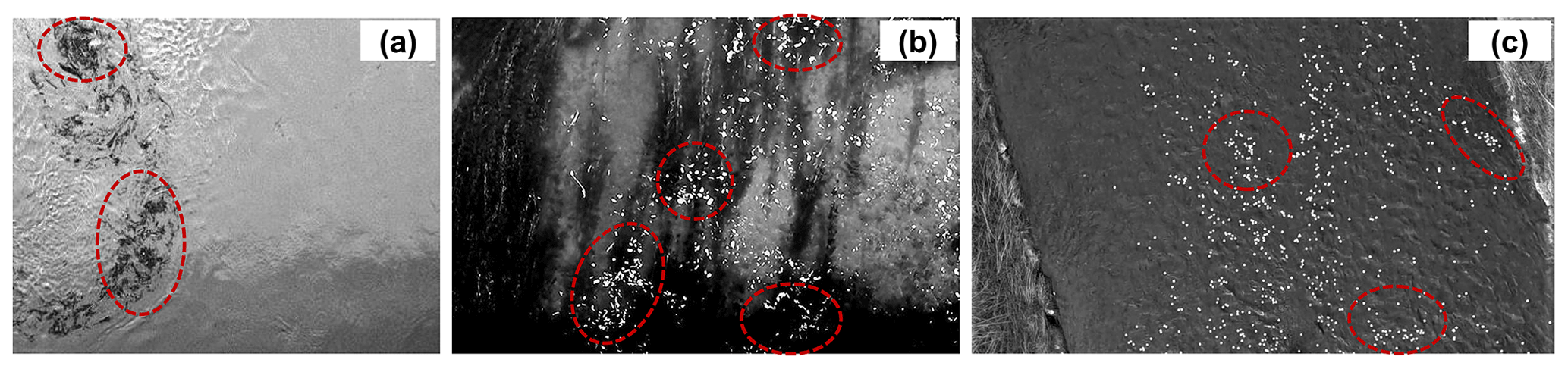
Figure 1Examples of moving and clustering structures on the water surface: (a) natural seeding during a flood event at the Tiber river, Italy (Tauro et al., 2017); (b, c) artificial seeding at low and intermediate flow conditions at Brenta river in Italy (Tauro et al., 2017) and Murg river in Switzerland (Detert et al., 2017), respectively.
The spatial distribution of artificial tracers (hereafter called spatial clustering) is, however, operator-dependent and influenced by their experience, the type of material deployed, and the amount. External environmental and river conditions such as wind and turbulence are also important factors. This issue is extremely relevant for discharge estimates recovered through image-based approaches because velocity errors are transmitted to streamflow estimates. As a consequence, and even when using up-to-date approaches, monitoring complex flows and extreme flood events is still a challenge.
This paper aims to quantify the accuracy of SFV estimates under different seeding densities and spatial-clustering levels. To achieve this goal, the following objectives were proposed: (i) perform numerical simulations of synthetic tracers to produce 33 600 synthetic images with known seeding characteristics; (ii) using these synthetic images, derive a functional relationship between seeding densities, spatial-clustering levels, and image-velocimetry errors under controlled conditions; (iii) analyse footage acquired from the Basento river to determine how variations in seeding characteristics such as seeding density and spatial clustering of tracers influence the image-velocimetry errors in a field environment. Finally, (iv) apply the function developed in (ii) to the Basento river to enable the selection of the optimal image frame sequence and minimise the velocity errors.
The rest of the paper is organised as follows: Sect. 2 presents the numerical framework for synthetic image generation; a description of the hydrological characteristics of the Basento case study, which is used as a proof of concept; and an outline of the PTV and PIV techniques adopted in the analysis. Section 3 analyses the effects of seeding density and spatial-clustering level on image-velocimetry results using the synthetically generated images and those of the Basento field case study. Section 4 presents the strengths and limitations of the research and framework adopted in this paper. Conclusions are provided in Sect. 5.
2.1 Numerical simulations
Numerical simulations were performed to test two different image-velocimetry algorithms under controlled conditions, minimising the effects of external disturbances. In particular, the influence of tracer or feature properties on the final errors was quantified. Synthetic tracers were randomly distributed in space with a unidirectional and constant velocity. They consist of uniform circular shapes with diameter Dxp≈10 px (pixels) and uniform white colour. Both diameters and colours – in greyscale intensity – were altered with white noise in order to consider more realistic configurations. Their spatial distribution was controlled by a generalised Poisson distribution (GPD) with an imposed numerical seeding density λ and spatial-clustering level υ.
The GPD was first introduced by Efron (1986), allowing the possibility to obtain point events randomly distributed in space with a given variance. The GPD has been used to model randomly distributed events in different studies and describe the spatial characteristics of the landscape and vegetation organisation across climatological gradients (e.g. Good et al., 2013; Manfreda et al., 2017). In this paper, the synthetic tracers are assumed to be randomly distributed in space with a mean number λS, where S is the considered area. As a consequence, the probability mass function that the random number of synthetic tracers N will be equal to a number ni is given by Eq. (1),
where λS and υ determine the location and the shape of fGPD(λS)(ni), and CGPD is an integration constant.
Tracers moved with a constant numerically imposed velocity of 15 px per frame along the y axis and within a grid of 500 px×500 px on a clear water background as representative of real environmental conditions. Tracer diameter was set to be larger than 2.5 px in order to avoid peak locking effects (Cardwell et al., 2011; Dal Sasso et al., 2018; Nobach et al., 2005). Typical tracer dimensions at laboratory and field scales motivated the choice of Dxp≈10 px for image-velocimetry experiments (Tauro et al., 2016).
Synthetic image sequences were generated by varying the number of tracers in the spatial domain, allowing the consideration of 14 different seeding densities ranging from ppp (particles per pixel) up to ppp. This range of variability was established based on the typical values adopted in field surveys (Tauro and Grimaldi, 2017) and numerical studies (Dal Sasso et al., 2018). Tracer colour (in terms of greyscale intensity) and diameter were altered (by introducing Gaussian white noise with standard deviations equal to 0.05 and 0.3, respectively) to simulate environmental signal noise such as possible changes in luminosity, brightness, and shadows. Figure 2 shows an example of synthetic images generated with different spatial-clustering levels and a fixed value of seeding density. In particular, the spatial distribution of tracers moves from an overdispersed organisation (υ=0.5), through a Poisson random distribution (υ=1) and an underdispersed one (υ=100), to a super underdispersed distribution (υ=200). Figure 2a–d present the original synthetic generation on the clear water background, while Fig. 2e–h show the preprocessed images, enhancing the contrast between tracers and background (see Sect. 2.3). Furthermore, each numerical experiment involved generating 20 images, and each configuration was run 10 times. The spatial-clustering level ranges from 0.5 to 200 (12 different values), and as a consequence, 33 600 synthetic images were generated (14 different λ, 12 different υ, 20 images per configuration, and each configuration 10 times).

Figure 2Synthetic generations of spatial distribution of tracers assuming different values of the parameter ν=0.5 (overdispersed distribution – a, e), 1.0 (Poisson random distribution – b, f), 100 (underdispersed distribution – c, g), and 200 (super underdispersed distribution – d, h). Fixed value of the seeding density . The generation was carried out adopting a background in the images to provide more realistic conditions (a–d). Thereafter, images have been preprocessed to increase the contrast and better visualise tracers (e–h).
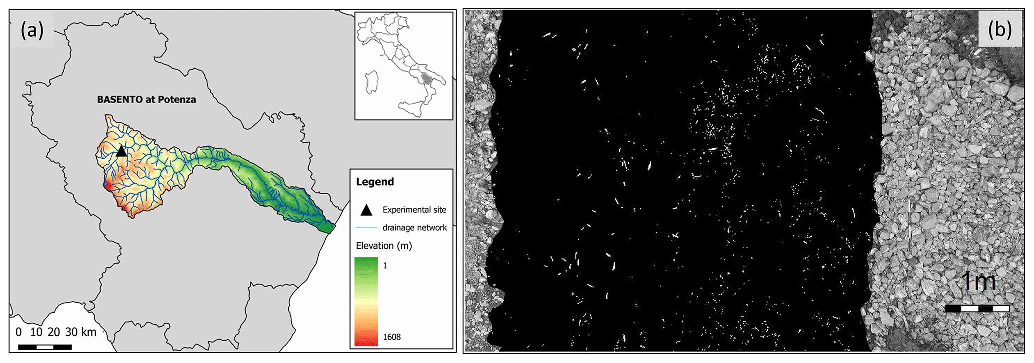
Figure 3(a) Basento river and its drainage basin with an indication of the measurement location (Basento at Potenza). (b) Greyscale footage acquired with a DJI Phantom 3 Pro (river banks) and corresponding footage after the preprocessing (river flow) aimed at enhancing contrast for particle identification.
2.2 Proof of concept: the Basento case study
A field survey on the Basento river (Basilicata region, southern Italy) was carried out to test the outcomes of numerical simulations under natural conditions. The cross section considered for the measurements is located in the upper portion of the basin (catchment area of about 127 km2; Fig. 3). The main river flow characteristics at the time of video acquisition were (i) river discharge (0.61 m3 s−1), (ii) maximum flow depth (0.38 m), (iii) river width (6.0 m), (iv) maximum surface flow velocity (0.68 m s−1), and (v) average surface flow velocity (0.40 m s−1). Data were acquired using a DJI Phantom 3 Professional Quadcopter (DJI, Shenzhen, China) equipped with an integrated 4k UHD (ultra-high-definition) video-recording camera and a three-axis stabilised system. Video acquisition was performed using a Sony EXMOR complementary metal oxide semiconductor (CMOS) sensor, and a greyscale video was captured from the UAS platform with a resolution of 1920 px×1080 px (i.e. full high definition, FHD). The frame rate was set to 24 frames per second (fps). Reference objects, useful for image scale calibration and stabilisation, were positioned at visible locations on the riverbanks. The calibration factor converting pixels to metres was estimated, taking into consideration those objects with known a priori dimensions. The ground sampling distance (GSD) was, therefore, computed as 0.005 m px−1. Benchmark velocity measurements were performed using a current meter (SEBA F1, SEBA Hydrometrie GmbH & Co, Kaufbeuren, Germany) in the proximity of the water surface at 11 different locations across the river cross section. The accuracy of measurements was within 2 % of the measured values, corresponding to 0.001 and 0.013 m s−1 for the minimum and maximum velocities in question. The spanning distance between the respective measurements was 0.5 m. Each measurement was made over a fixed acquisition period of 30 s. River discharge was estimated according to ISO 748 (1997) using the velocity–area method. The cross section was divided into panels of equal width, and, for each panel, the velocity was measured at 20 %, 60 %, and 80 % of the panel depth. Artificial seeding was deployed onto the water surface, giving the possibility to create complex floating structures. Two operators were involved in the process, and artificial tracers made of wood chips were used to enhance particle seeding in the region of interest (ROI).
The videos captured with the UAS were first stabilised using an automatic feature selection method that identifies features in frame pairs, matching them to compute possible values of translation and rotation. The Features from Accelerated Segment Test (FAST) detection algorithm was applied to identify features in an ad hoc ROI. To improve the feature-matching accuracy at each step, the method utilises the random sample consensus (RANSAC) filter to remove unacceptable correspondences. The application of the stabilisation algorithm allowed the effects of camera movements to be reduced throughout the duration of the video. Planar errors considering differences in translation and rotation were computed, taking the first frame as the reference target. On average, the reduction due to the stabilisation process goes from 64 to 7 px for the Basento case study. Therefore, movement in the original video is reduced by around 89 %. The stabilisation algorithm does not require ground control points (GCPs) to be applied. Rather, it performs the detection of features automatically, making the stabilisation process a good alternative for unexperienced users.
The Basento river presented low-flow conditions, leading us to subsample the original video from 24 to 12 fps. The choice of the appropriate frame rate was made to ensure, on the one hand, a frame-by-frame displacement bigger than the particle dimensions and, on the other hand, to minimise the effects of camera movement between frame pairs on the calculation of surface velocity. The footage was acquired in greyscale, and a preprocessing procedure was applied using contrast-stretching techniques to enhance the visibility of the artificial tracers against the background. For this purpose, GIMP (the GNU Image Manipulation Program) was utilised to adjust brightness and contrast. This procedure eliminated a large amount of noise caused by external reflections, improving the number of tracers identified and thus cross-correlation in the ROI. Figure 3b shows a composite example of the original frame in greyscale, overlain by a preprocessed image covering the extent of the active channel (darker area overlapping the original frame).
2.3 Image-velocimetry analysis
PTV analyses were carried out by employing a command-line version of PTVLab software (Brevis et al., 2011) that was automated in order to handle the number of synthetic images. Tracer detection was performed using the particle Gaussian mask correlation method (Ohmi and Li, 2000). Parameters for particle diameter and reflectance intensity were set equal to 8 px and 70, respectively. Particle tracking was implemented using a cross-correlation algorithm (Wu and Pairman, 1995). The interrogation area (IA) was set at 20 px, cross-correlation threshold at 0.7, and neighbour similarity percentage at 25 %. PTV parameter settings were slightly modified under field conditions due to the differences between the numerical and field datasets. In particular, the average tracer dimension in the field conditions was estimated as 5 px, and therefore, the particle diameter was set equal to 4 px and the IA to 25 px.
PIV analyses were performed by employing a command-line version of PIVLab software (Thielicke and Stamhuis, 2014). The PIV algorithm was applied for both numerical and field analysis using the fast Fourier transform (FFT) with a three-pass standard correlation method (search and interrogation areas of 128 px×64 px, 64 px×32 px, and 32 px×16 px and with 50 % overlap). Additionally, the 2 point × 3 point Gaussian fit was employed to estimate the subpixel displacement peak. These parameters were carefully chosen to ensure correct identification and tracking of synthetic tracers.
Finally, the quality of the results was determined by examining the magnitude of the errors that were computed as
where uC is the computed velocity, and uR is the numerically imposed (numerical case taken as reference) or measured (field case) velocity.
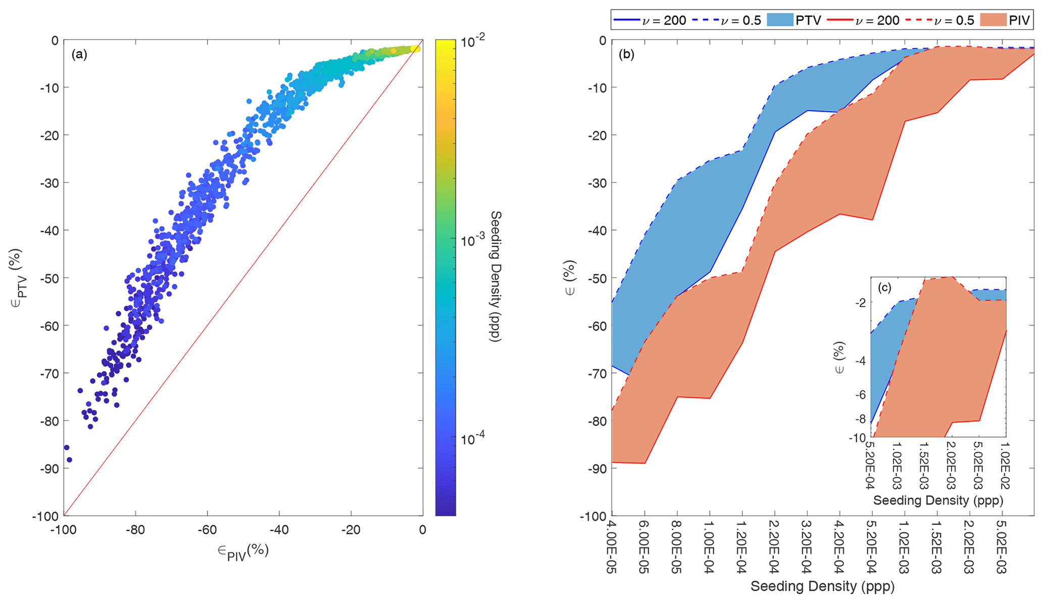
Figure 4Comparison of PTV and PIV results using synthetic images with different values of seeding density and spatial-clustering level. Only negative errors were observed with numerical results. (a) PTV vs. PIV errors (ϵPTV and ϵPIV, respectively). Each data point is associated with a colour that is scaled based on the numerically imposed seeding density adopted in the numerical generation of synthetic images. (b) Envelope error curves and areas as a function of seeding density and level of spatial clustering ν. The blue and orange colours are associated with PTV and PIV results, respectively. Dashed and solid lines are associated with ν=0.5 and ν=200, respectively. (c) Close-up of the upper-right portion of (b).
3.1 Numerical analysis
The performance of PTV and PIV tracking algorithms was assessed by the calculation of errors (considering the imposed numerical surface velocity) to test how the seeding density and spatial distribution of tracers influenced the final velocity estimates. No postprocessing method was applied to filter the spatio-temporal velocity results. The ROI was taken as the original dimension of the synthetic image generation, i.e. 500 px×500 px. The processing times, considering all the synthetically generated images, for PTV and PIV analyses were 18 548 and 4736 s, respectively. The same hardware (i7-8700 CPU at 3.20 GHz and 32 GB RAM) was used for both image-velocimetry analyses, leading to a fair comparison between them. PTV computing time was almost 4 times higher than PIV under the circumstances considered in this study. For all cases, PTV and PIV techniques systematically underestimated the imposed numerical velocity independently of the seeding density and spatial-clustering level under consideration. Consequently, only negative errors were observed with numerical results, in agreement with previously published work (Dal Sasso et al., 2018). This can be due to the use of a static background that may introduce sporadic zero-velocity vectors. Figure 4 shows the PTV and PIV error results with different values of seeding densities and spatial-clustering levels. A comparison between PTV and PIV is shown in Fig. 4a, where each data point is associated with a colour that is scaled based on the numerically imposed seeding density adopted in the generation of synthetic images. A strong dependence between image-velocimetry results and seeding density was observed: errors can be reduced by increasing the seeding density. In all cases, PTV outperformed PIV under the synthetic conditions analysed in this study. These findings also support those of Tauro et al. (2017), who found that PTV outperformed PIV in two different field case studies (Brenta and Tiber rivers). It is, however, noteworthy that the results we present here refer to a single synthetic experiment that, although realistic, is not representative of any field condition. Therefore, further investigation with a larger set of idealised and field circumstances should be carried out to generalise the obtained results.
Figure 4b shows the envelope error curves (and areas between them) for a range of seeding densities and level of spatial clustering ν. The blue and orange colours are associated with PTV and PIV error results, while dashed and solid lines are associated with ν=0.5 and ν=200, respectively. For the sake of simplicity, Fig. 4b only shows the extreme cases, when ν=0.5 and ν=200; nevertheless, all the other cases (with ν values between these two extremes) were confined within these envelope curves. Error results of both techniques were influenced by ν, with a higher spatial-clustering level tending to deteriorate the accuracy of image-velocimetry results, producing higher errors and associated variability across the range of seeding densities. When the sensitivities of PIV and PTV to changes in ν are compared, PIV is generally more sensitive than PTV, as demonstrated by the greater distance between ν=0.5 and ν=200 lines for a given seeding density and by the shaded orange area being greater than the blue. The minimum seeding density leading to the lowest errors (around 2 %–3 %) depended on ν. These errors were taken as reference values after which an asymptotic behaviour was observed. As a consequence, this minimum seeding density concept is termed reference seeding density in the rest of the paper. For instance, considering the PIV case, the reference seeding density values were and ppp for ν=0.5 and ν=200, respectively. The reference seeding density values for PTV were and ppp for ν=0.5 and ν=200, respectively.
These numerical results are useful to visualise more-in-depth trends under controlled flow conditions, avoiding external disturbances. Results demonstrated that the minimum required seeding density to produce an error equal to or lower than 3 % differs slightly between the two techniques. We used this percentage as a reference error in order to derive a reference seeding density associated with a known error. It was observed that PIV required ppp, while PTV needed about ppp to reach the same error. Notably, seeding densities lower than ppp produced larger errors (larger than 3 %), and consequently, flows should be seeded at least at this density in field campaigns for optimal implementation of the methods. This practice should be adopted if at all possible since typical natural flows are not characterised by abundant transiting features, with maybe the exception of high flows. Furthermore, the effective seeding density (defined as the seeding that the algorithms are genuinely able to identify, match, and track) is always lower than the one transiting onto the water surface, and therefore, extra seeding is recommended practice. However, we are aware that this recommendation might not be practical in all conditions since fixed cameras can operate remotely without the necessity to be in person at the field site, and deploying material in wide channels or difficult-to-access areas might be challenging.
Following dimensional considerations, a model of the image-based errors can be formulated. Since the only variables considered in this study were the spatial-clustering level and the seeding density, it is hypothesised that these errors depend on only these variables. In functional form, this gives
where f is a generic function, and ρ and ρcν1 are the seeding density and the reference seeding density at ν=1 (Poisson case taken as a reference). According to the Buckingham π theorem, Eq. (3) can be rewritten in terms of dimensionless parameters as follows:
The function f is usually considered as a multiplication of power laws (Buckingham, 1914; Evans, 1972; Melville and Sutherland, 1988; Pizarro et al., 2017b). In this study, we partially follow this approach and also hypothesise that the functional relationship f is described by a two-parameter exponential function:
where the SDI (Seeding Distribution Index) is the multiplication of power laws, and c1, c2, k1, and k2 are fitting coefficients. Model performance was quantified by means of the root mean square error (RMSE) and the Nash–Sutcliffe efficiency (NSE) for prediction of the image-velocimetry errors. In turn, the fitting coefficients were calibrated using the MATLAB genetic algorithm optimising RMSE. Table 1 summarises the results of the calibration process for both PTV and PIV, while Fig. 5 shows the image-velocimetry errors as a function of the SDI and observed versus computed errors. Figure 5 indicates that the SDI can correctly reproduce the main dynamics of the image-velocimetry errors, reporting low RMSE values in calibration (5.34 % and 5.77 % for PIV and PTV, respectively). A visual inspection of Fig. 5a and b shows that increasing SDI values leads to higher errors for both image-velocimetry techniques. Figure 5b and d also show that the predictive capacity of Eq. (5) is higher at low PTV and PIV error values.
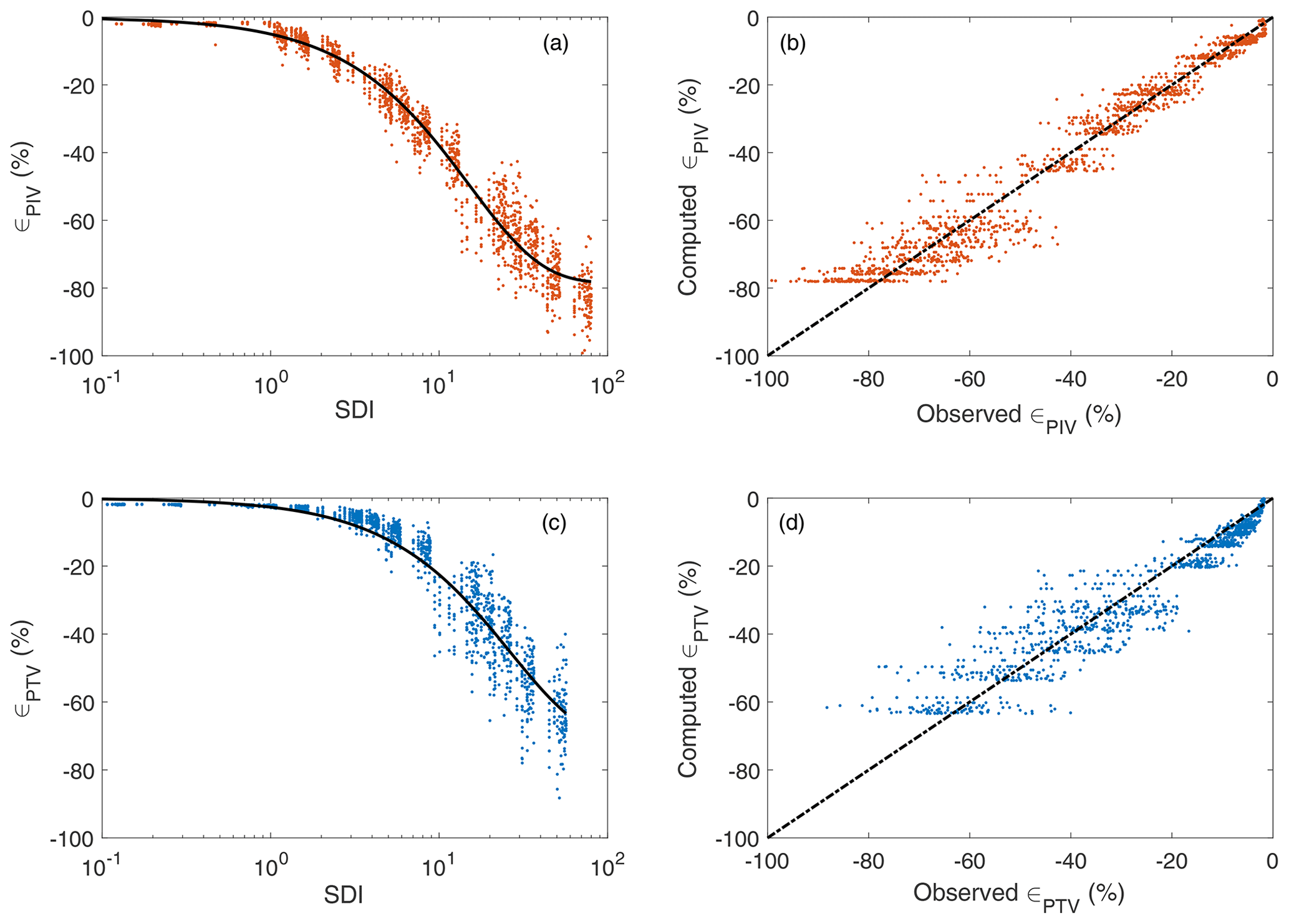
Figure 5Image-velocimetry errors as a function of the SDI (a, c) and observed versus computed errors (b, d). Blue and orange colours are related to PTV and PIV numerical error results. Solid lines represent Eq. (5), while the dashed lines are the perfect agreement between observed and computed image-velocimetry errors.
Table 1Calibrated values of c1, c2, k1, k2 and model performances in terms of RMSE (%) and NSE. ρcν1 values for PIV and PTV were taken from Fig. 4 and are and ppp, respectively.
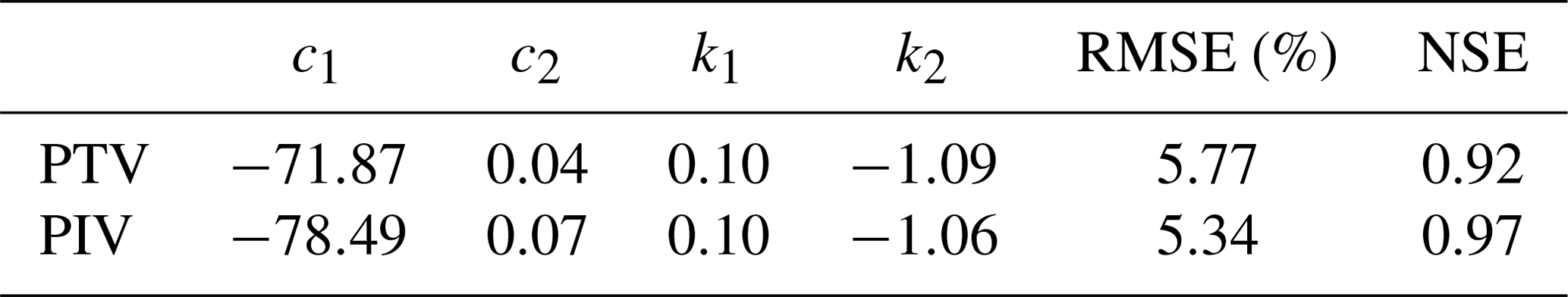
Even though PIV and PTV work differently, the fitted values in Eq. (5) were similar. Remarkably, k1 and k2 showed that the dimensionless SDI parameter can be approximated and used in practice as
Furthermore, considering that the errors are minimised when the SDI takes low values, the SDI can be used in field conditions as a descriptor to choose the optimal portion of a video to analyse in order to minimise the errors in image-velocimetry estimates as a function of seeding density and spatial-clustering level. This novel idea is explored in the next subsection, taking the Basento river as a proof-of-concept case study.
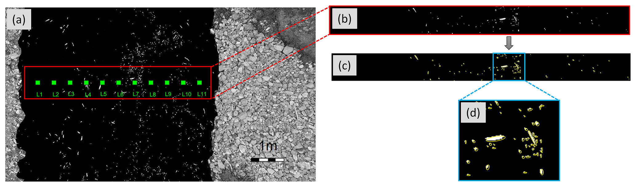
Figure 6(a) Preprocessed frame indicating the ROI and the reference measuring locations for benchmark purposes. The isolation of the ROI is presented in (b), while an example of identified features on the water surface is presented in (c). (d) Close-up of an arbitrary portion of the ROI with the identified features.
3.2 Field campaign: the Basento case study
Outcomes of the numerical analysis were tested on a real case study in order to identify the best temporal window (i.e. a subset of the video sequence) for image-velocimetry analyses. The case study was selected due to the spatial distribution of tracers varying significantly during the recording period, making it subjective to manually select the optimal frames for analysis. Figure 6 displays a preprocessed frame with the location of the measuring points using standard field equipment (from L1 to L11). These surface flow velocity measurements were taken as reference velocities for PTV and PIV benchmarking. Figure 6b and c show a close-up of the ROI and the identification of transiting features, respectively. An example of identified features is presented in Fig. 6d. In this figure, the number of features, their relative positions, and associated areas were identified using an ad hoc algorithm developed by Dal Sasso et al. (2020). Moving features – that can be blobs, regions of uniform intensity, or local corners – are detected and processed to derive seeding properties (i.e. empirical seeding densities and spatial distribution of tracers) on a frame-by-frame basis even if shapes and dimensions of the tracers vary considerably. Using this approach, the empirical spatial-clustering level (i.e. the empirical equivalent to that used in the numerical simulations), was quantified through the spatial dispersion index (, where Var(N) and E(N) are the variance and mean values of the number of tracers N, respectively, computed in sub-patches of the same size). This metric is normally measured to quantify whether a set of events are clustered or dispersed. Important to notice, D* is assumed as an estimator of ν due to their similar properties such as , which means features follow a Poisson distribution, while and follow an over- and underdispersed spatial distribution, respectively.

Figure 7Overview of seeding characteristics in the ROI of the Basento river during the acquisition time: (a) seeding density in particles per pixel, (b) dimensionless dispersion index D*.
Figure 7 shows a comprehensive overview of the seeding behaviour during the 200 frames considered for the analysis. Figure 7a and b present the seeding density in particles per pixel and the dispersion index D* computed as a function of the frame number. The minimum and maximum values for seeding density were and ppp, while those for the dispersion index were 4.1 and 57.3. Additionally, the estimated mean area of features (computed frame by frame and inside the ROI) varied between approximately 1.5 and 3.5 cm2.
The approach mentioned above made it possible to compute the SDI and correctly identify the worst and best part of the video for image-velocimetry analysis. A moving frame window length of 100 frames was arbitrarily chosen, on which an average dispersion index D* and seeding density were computed. This decision was motivated to increase the odds of populating the entire ROI with features. The empirical SDI was then calculated as , where and are the average-in-100-frames dispersion index and seeding density, respectively. Figure 8a depicts the SDI as a function of the frame windows. Triangle markers correspond to the minimum and maximum values of the SDI and their respective locations (82–181 and 1–100, respectively). Figure 8a shows the particular case of PTV; nevertheless, PIV presented similar results. The locations of the minimum and maximum SDI values were, therefore, unaffected by the image-velocimetry technique under consideration.
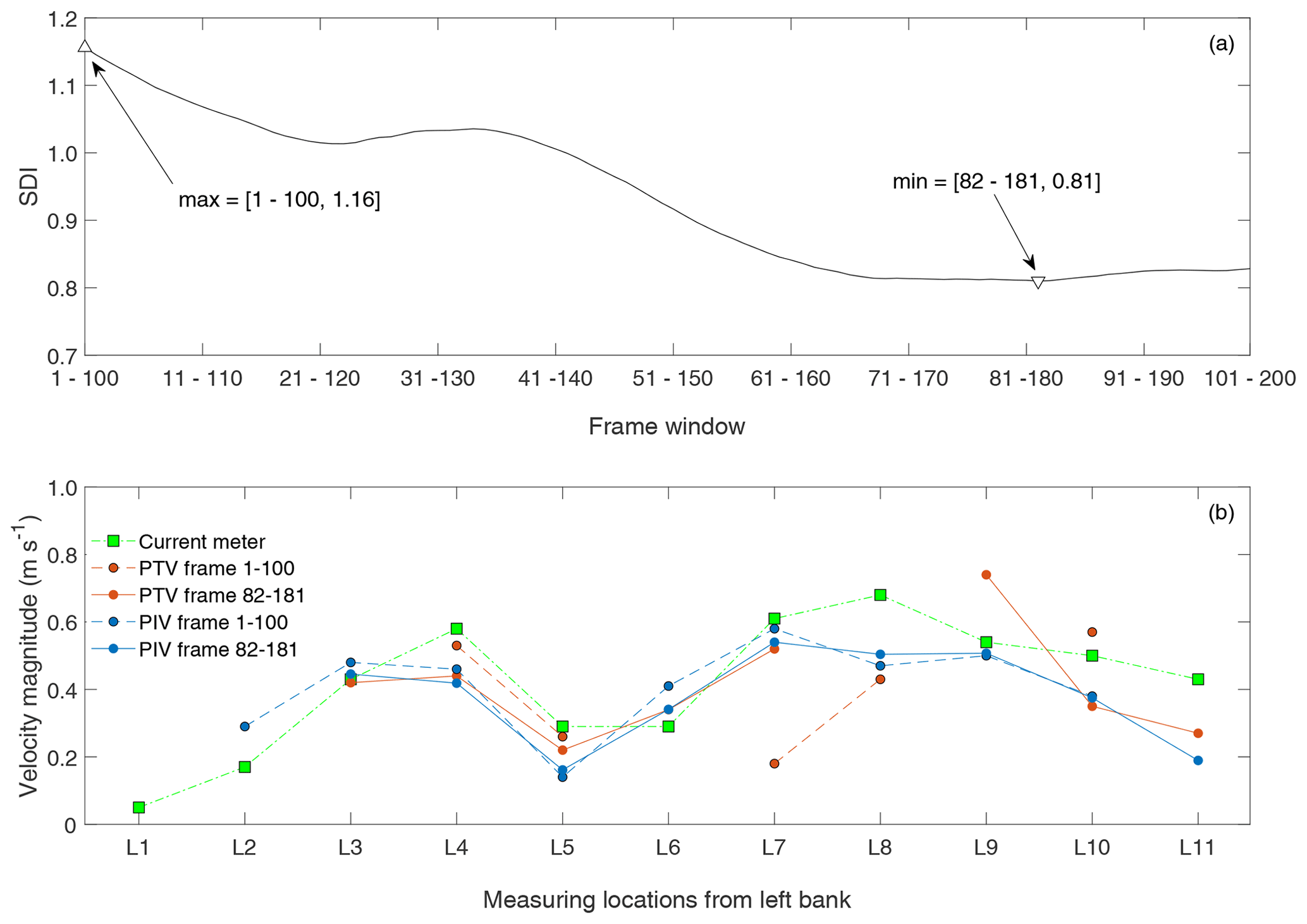
Figure 8(a) The SDI as a function of the frame window considering 100 frames. Triangle markers correspond to the minimum and maximum value of the SDI. Their locations were 82–181 and 1–100, respectively. Particular case of PTV, whereas PIV showed similar results, and the locations of the minimum and maximum SDI values were unaffected by the image-velocimetry technique. (b) Comparison between PTV and PIV data for experiments on the Basento river. Values recorded with the current meter are also reported for a rapid visual assessment (green squares). Blue and orange colours represent PIV and PTV data.
Image-based velocity results were averaged in a block of 30×30 cm2 for a fair comparison among PTV, PIV, and benchmark velocity values. The measuring locations corresponded with the centre of the blocks. Computed velocities across the cross section and reference velocities are reported in Fig. 8b. The blue and orange colours are associated with PTV and PIV results, respectively (same colours used within numerical results for consistency and fast visual comparison). Green squares are the velocities measured using the current meter. Notably, the measuring location L1 had no computed velocity values due to the lack of features transiting on this part of the ROI, whereas only PIV was able to compute velocities at L2. This issue can be explained due to the inherent property of PIV to identify and track non-seeded features such as ripples and other structures transiting on the water surface. Interestingly, and in agreement with numerical results, 80 % (frames 1–100) and 75 % (frames 82–182) of the computed velocity measuring locations underestimated the reference velocities using PTV. Similarly, results using PIV were 67 % and 78 %, respectively. Therefore, a close agreement was observed with the numerical results that systematically presented underestimations of computed velocities in comparison with the numerically imposed one. The computed errors using PTV and PIV on the total number of frames available were 23.93 % and 23.69 %, respectively. Moreover, adopting the optimal frame window ensured that image-velocimetry measurements were produced for a greater or equal proportion of the channel than that produced by using frames 1–100 (PTV: 72.7 % vs. 45.5 % of the channel width; PIV: 81.8 % vs. 81.8 %).
Both image-velocimetry approaches correctly captured the mean behaviour of velocities across the cross section. Table 2 presents summarised information of the average-in-100-frames seeding density and dispersion index as well as the initial and final frame used for image-velocimetry purposes. The SDI value is also presented as well as the absolute average error across the cross section. As expected from numerical analyses, an error reduction with respect to the worst scenario of about 15.9 % (PTV) and 16.1 % (PIV) was found in the Basento case study by employing the optimal frame window that minimises the SDI. It is therefore recommended that the SDI is used as a descriptor of the optimal portion of a video to analyse.
Table 2Overview of feature characteristics, minimum and maximum SDI values, and absolute errors using PTV and PIV. Values in parentheses correspond to the error reduction with respect to the worst scenario using the optimal frame window.
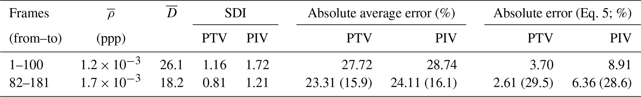
Finally, considering numerical findings, field image-based estimates presented larger errors in comparison with numerical results for the respective same values of the SDI (last two columns of Table 2). This is despite the average seeding density being relatively high ( ppp) and the average dispersion index being relatively low (∼20). Possible reasons for deteriorations in PTV and PIV estimates can be attributed to other variables such as video stabilisation issues, noise due to different environmental conditions (e.g. intermittent and different levels of illumination, water reflections, and presence of shadows), and different shapes and dimensions of features (stressing the matching and tracking process between consecutive frames). In this regard, Dal Sasso et al. (2020) recently introduced metrics for the quantification of seeding characteristics needed to enhance image-velocimetry performances in rivers. Among them, the seeding density, spatial-clustering level, and coefficient of variation of tracers' dimensions were statistically significant predictors of velocity estimation accuracy. These issues should be the subject of further investigation, along with the application of these ideas to case studies with very different field conditions, to assess the uncertainty of computed surface velocities and remote river flow estimates.
One of the main strengths of this study is the introduction of the new dimensionless SDI, which combines seeding characteristics – seeding density and spatial clustering of tracers – for image-velocimetry purposes. A numerical framework of synthetically generated images was adopted to isolate seeding effects on the performance of PIV and PTV analysis. This numerical framework allowed the generation of moving tracers with the possibility to vary the seeding density and spatial clustering of tracers. Additionally, one field case study was used to test and validate numerical findings. However, among other limitations, the numerical framework considered a constant and unidirectional imposed velocity only. Besides, PIV and PTV were set to run using a single configuration (e.g. PIV used FFT with a three-pass correlation method and fixed search and interrogation areas rather than other combinations of them or an ensemble correlation method). The field case study was artificially seeded to enhance the identification and tracking of moving patterns on the water surface. Interestingly, the dispersion index D* was used as an empirical estimator of the numerical clustering level of tracers ν. D* and ν share some interesting properties, which are useful to characterise under- and overdispersed spatial distribution of tracers in practical applications. Finally, the errors computed using all frames available (frames 1–200) versus the optimal frame window (frames 82–181) were of the same order of magnitude even though the number of frames used with the SDI was half of the total available. As a consequence, the quality of the seeding characteristics seemed to be more critical than the duration of the footage. Of course, many other factors might affect the quality of the videos and, consequently, the performance of image-velocimetry estimates, but this assessment focuses specifically on the spatial distribution of tracers. In the field, other factors such as illumination conditions, shading on the scene, light reflections, presence of turbulent fluxes, and vibration of the camera, among others, could further affect overall quality of the analysis, and these should be the subject of further assessment.
In this paper, we investigated the performances of PTV and PIV for surface flow velocity estimation. Synthetic generation of 33 600 images was performed to test image-velocimetry techniques under different levels of seeding density and tracer spatial clustering. In all numerical cases, velocity results systematically underestimated the imposed numerical velocity. A general trend was observed in which increasing the seeding density and decreasing the level of spatial clustering improved results. The main advantage of the numerical approach adopted is the controlled conditions in which the analyses can be conducted, minimising the effects of external disturbances. Based on numerical findings, seeding densities lower than ppp produced larger errors, and consequently, flows should be extra-seeded in field campaigns for optimal implementation of image-velocimetry methods. Additionally, the dimensionless SDI was introduced as a descriptor of the optimal portion of the video to analyse using the studied image-based techniques. Based on numerical results, the SDI can be approximated and used in practice as , where ν, ρ, and ρcν1 are the spatial-clustering level, the seeding density, and the converging seeding density at ν=1, respectively. A reduction in image-based errors was observed with lower values of the SDI.
The Basento field case study (located in southern Italy) was considered as a proof of concept of the proposed framework. Seeding characteristics were empirically estimated using a novel algorithm recently developed by the authors, opening the possibilities of more refined analyses. The number of features, relative positions, and associated areas were saved for the computation of the empirical seeding densities and spatial-clustering levels. The empirical SDI values were then computed, and two extreme cases were considered for velocimetry comparison purposes: (i) the one considering the maximum value of the SDI (worst case) and (ii) the one related to the minimum SDI (best case). Field results corroborated numerical findings, and an error reduction of about 15.9 % and 16.1 % was achieved for PTV and PIV approaches, respectively, by using the optimal frame window that minimises the SDI for the Basento case study.
Interestingly, field image-based estimates presented larger errors than numerical results for the respective same values of the SDI. Possible reasons for deteriorating PTV and PIV estimates can be attributed to other variables such as (i) video stabilisation issues; (ii) variable levels of illumination, water reflections, and presence of shadows; and (iii) different shapes and dimensions of seeding features, stressing the importance of the feature-matching and feature-tracking process between consecutive frames. Further assessment is required to evaluate the significance of these factors in contributing to the uncertainty in image-velocimetry estimates across a range of hydrological and environmental conditions.
The code used to compute the SDI as well as seeding metrics is available in Pizarro et al. (2020b): https://doi.org/10.17605/OSF.IO/8EGQW.
Numerical and field data used in this study are available in Pizarro et al. (2020a): https://doi.org/10.5281/zenodo.3761859.
AP conceptualised the study, wrote the scripts, processed and analysed the data, and drafted the paper. SFDS analysed the field data. SM coordinated the research activities and defined the research project. SFDS, MTP, and SM contributed to the writing and reviewed the manuscript.
The authors declare that they have no conflict of interest.
This work was funded by the COST Action CA16219 “HARMONIOUS – Harmonization of UAS techniques for agricultural and natural ecosystems monitoring”.
This research has been supported by the European Cooperation in Science and Technology (grant no. CA16219).
This paper was edited by Nunzio Romano and reviewed by Evangelos Rozos and two anonymous referees.
Adrian, R.: Particle-Imaging Techniques For Experimental Fluid-Mechanics, Annu. Rev. Fluid Mech., 23, 261–304, https://doi.org/10.1146/annurev.fluid.23.1.261, 1991.
Adrian, R. J.: Twenty years of particle image velocimetry, Exp. Fluids, 39, 159–169, 2005.
Anderson, K. E., Paul, A. J., McCauley, E., Jackson, L. J., Post, J. R., and Nisbet, R. M.: Instream flow needs in streams and rivers: The importance of understanding ecological dynamics, Front. Ecol. Environ., 4, 309–318, https://doi.org/10.1890/1540-9295(2006)4[309:IFNISA]2.0.CO;2, 2006.
Batalla, R. J. and Vericat, D.: Hydrological and sediment transport dynamics of flushing flows: Implications for management in large Mediterranean rivers, River Res. Appl., 25, 297–314, https://doi.org/10.1002/rra.1160, 2009.
Bechle, A., Wu Chin, H., Liu, W.-C., and Kimura, N.: Development and Application of an Automated River-Estuary Discharge Imaging System, J. Hydraul. Eng., 138, 327–339, https://doi.org/10.1061/(ASCE)HY.1943-7900.0000521, 2012.
Brevis, W., Niño, Y., and Jirka, G. H.: Integrating cross-correlation and relaxation algorithms for particle tracking velocimetry, Exp. Fluids, 50, 135–147, 2011.
Buckingham, E.: On physically similar systems; Illustrations of the use of dimensional equations, Phys. Rev., 4, 345–376, https://doi.org/10.1103/PhysRev.4.345, 1914.
Cardwell, N. D., Vlachos, P. P., and Thole, K. A.: A multi-parametric particle-pairing algorithm for particle tracking in single and multiphase flows, Meas. Sci. Technol., 22, 105406, https://doi.org/10.1088/0957-0233/22/10/105406, 2011.
Dal Sasso, S. F., Pizarro, A., Samela, C., Mita, L., and Manfreda, S.: Exploring the optimal experimental setup for surface flow velocity measurements using PTV, Environ. Monit. Assess., 190, 460, https://doi.org/10.1007/s10661-018-6848-3, 2018.
Dal Sasso, S. F., Pizarro, A., and Manfreda, S.: Metrics for the quantification of seeding characteristics to enhance image velocimetry performance in rivers, Remote Sens., 12, 1789, https://doi.org/10.3390/rs12111789, 2020.
Detert, M., Johnson, E. D., and Weitbrecht, V.: Proof-of-concept for low-cost and non-contact synoptic airborne river flow measurements, Int. J. Remote Sens., 38, 2780–2807, https://doi.org/10.1080/01431161.2017.1294782, 2017.
Efron, B.: Double exponential families and their use in generalized linear regression, J. Am. Stat. Assoc., 81, 709–721, https://doi.org/10.1080/01621459.1986.10478327, 1986.
Eltner, A., Sardemann, H., and Grundmann, J.: Technical Note: Flow velocity and discharge measurement in rivers using terrestrial and unmanned-aerial-vehicle imagery, Hydrol. Earth Syst. Sci., 24, 1429–1445, https://doi.org/10.5194/hess-24-1429-2020, 2020.
Evans, J. H.: Dimensional Analysis and the Buckingham Pi Theorem, Am. J. Phys., 40, 1815–1822, https://doi.org/10.1119/1.1987069, 1972.
Fujita, I., Muste, M., and Kruger, A.: Large-scale particle image velocimetry for flow analysis in hydraulic engineering applications, J. Hydraul. Res., 36, 397–414, 1998.
Good, S. P., Rodriguez-Iturbe, I., and Caylor, K. K.: Analytical expressions of variability in ecosystem structure and function obtained from threedimensional stochastic vegetation modelling, P. Roy. Soc. A, 469, 20130003, https://doi.org/10.1098/rspa.2013.0003, 2013.
Huang, W. C., Young, C. C., and Liu, W. C.: Application of an automated discharge imaging system and LSPIV during typhoon events in Taiwan, Water, 10, 280, https://doi.org/10.3390/w10030280, 2018.
ISO 748: Measurement of Liquid Flow in Open Channel – Velocity-Area Methods, 1997.
Kinzel, P. J. and Legleiter, C. J.: sUAS-based remote sensing of river discharge using thermal particle image velocimetry and bathymetric lidar, Remote Sens., 11, 2317, https://doi.org/10.3390/rs11192317, 2019.
Le Coz, J., Hauet, A., Pierrefeu, G., Dramais, G., and Camenen, B.: Performance of image-based velocimetry (LSPIV) applied to flash-flood discharge measurements in Mediterranean rivers, J. Hydrol., 394, 42–52, 2010.
Leitão, J. P., Peña-Haro, S., Lüthi, B., Scheidegger, A., and Moy de Vitry, M.: Urban overland runoff velocity measurement with consumer-grade surveillance cameras and surface structure image velocimetry, J. Hydrol., 565, 791–804, https://doi.org/10.1016/j.jhydrol.2018.09.001, 2018.
Lloyd, P. M., Stansby, P. K., and Ball, D. J.: Unsteady surface-velocity field measurement using particle tracking velocimetry, J. Hydraul. Res., 33, 519–534, 1995.
Manfreda, S.: On the derivation of flow rating curves in data-scarce environments, J. Hydrol., 562, 151–154, https://doi.org/10.1016/j.jhydrol.2018.04.058, 2018.
Manfreda, S., Caylor, K. K., and Good, S. P.: An ecohydrological framework to explain shifts in vegetation organization across climatological gradients, Ecohydrology, 10, e1809, https://doi.org/10.1002/eco.1809, 2017.
Manfreda, S., Link, O., and Pizarro, A.: A theoretically derived probability distribution of scour, Water, 10, 1520, https://doi.org/10.3390/w10111520, 2018a.
Manfreda, S., McCabe, M. F., Miller, P. E., Lucas, R., Madrigal, V. P., Mallinis, G., Dor, E. B., Helman, D., Estes, L., Ciraolo, G., Müllerová, J., Tauro, F., de Lima, M. I., de Lima, J. L. M. P., Maltese, A., Frances, F., Caylor, K., Kohv, M., Perks, M., Ruiz-Pérez, G., Su, Z., Vico, G., and Toth, B.: On the use of unmanned aerial systems for environmental monitoring, Remote Sens., 10, 641, https://doi.org/10.3390/rs10040641, 2018b.
Manfreda, S., Pizarro, A., Moramarco, T., Cimorelli, L., Pianese, D., and Barbetta, S.: Potential advantages of flow-area rating curves compared to classic stage-discharge-relations, J. Hydrol., 585, 124752, https://doi.org/10.1016/j.jhydrol.2020.124752, 2020.
Melville, B. W. and Sutherland, A. J.: Design method for local scour at bridge piers, J. Hydraul. Eng., 114, 1210–1226, 1988.
Muste, M., Fujita, I., and Hauet, A.: Large-scale particle image velocimetry for measurements in riverine environments, Water Resour. Res., 44, W00D19, https://doi.org/10.1029/2008WR006950, 2008.
Nobach, H., Damaschke, N., and Tropea, C.: High-precision sub-pixel interpolation in particle image velocimetry image processing, Exp. Fluids, 39, 299–304, 2005.
Ohmi, K. and Li, H.-Y.: Particle-tracking velocimetry with new algorithms, Meas. Sci. Technol., 11, 603–616, https://doi.org/10.1088/0957-0233/11/6/303, 2000.
Owe, M.: Long-term streamflow observations in relation to basin development, J. Hydrol., 78, 243–260, 1985.
Pearce, S., Ljubičić, R., Peña-Haro, S., Perks, M., Tauro, F., Pizarro, A., Dal Sasso, S., Strelnikova, D., Grimaldi, S., Maddock, I., Paulus, G., Plavšić, J., Prodanović, D., and Manfreda, S.: An Evaluation of Image Velocimetry Techniques under Low Flow Conditions and High Seeding Densities Using Unmanned Aerial Systems, Remote Sens., 12, 232, https://doi.org/10.3390/rs12020232, 2020.
Perks, M., Sasso, S. F. D., Hauet, A., Le Coz, J., Pearce, S., Peña-Haro, S., Tauro, F., Grimaldi, S., Hortobágyi, B., Jodeau, M., Maddock, I., Pénard, L., and Manfreda, S.: Towards harmonization of image velocimetry techniques for river surface velocity observations, Earth Syst. Sci. Data, 12, 1545–1559, https://doi.org/10.5194/essd-12-1545-2020, 2020.
Perks, M. T., Russell, A. J., and Large, A. R. G.: Technical Note: Advances in flash flood monitoring using unmanned aerial vehicles (UAVs), Hydrol. Earth Syst. Sci., 20, 4005–4015, https://doi.org/10.5194/hess-20-4005-2016, 2016.
Peterson, S. D., Chuang, H. S., and Wereley, S. T.: Three-dimensional particle tracking using micro-particle image velocimetry hardware, Meas. Sci. Technol., 19, 115406, https://doi.org/10.1088/0957-0233/19/11/115406, 2008.
Pizarro, A., Samela, C., Fiorentino, M., Link, O., and Manfreda, S.: BRISENT: An Entropy-Based Model for Bridge-Pier Scour Estimation under Complex Hydraulic Scenarios, Water, 9, 889, https://doi.org/10.3390/w9110889, 2017a.
Pizarro, A., Ettmer, B., Manfreda, S., Rojas, A., and Link, O.: Dimensionless effective flow work for estimation of pier scour caused by flood waves, J. Hydraul. Eng., 143, 06017006, https://doi.org/10.1061/(ASCE)HY.1943-7900.0001295, 2017b.
Pizarro, A., Dal Sasso, S. F., Perks, M. T., and Manfreda, S.: Data on spatial distribution of tracers for optical sensing of stream surface flow (Version 0.1), [Dataset], Zenodo, https://doi.org/10.5281/zenodo.3761859, 2020a.
Pizarro, A., Dal Sasso, S. F., Perks, M. T., and Manfreda, S.: Identifying the optimal spatial distribution of tracers for optical sensing of stream surface flow (Version 0.1), [codes], OSF, https://doi.org/10.17605/OSF.IO/8EGQW, 2020b.
Raffel, M., Willert, C. E., Scarano, F., Kähler, C. J., Wereley, S. T., and Kompenhans, J.: Particle image velocimetry: a practical guide, Springer, Cham, Switzerland, 2018.
Strelnikova, D., Paulus, G., Käfer, S., Anders, K.-H., Mayr, P., Mader, H., Scherling, U., and Schneeberger, R.: Drone-Based Optical Measurements of Heterogeneous Surface Velocity Fields around Fish Passages at Hydropower Dams, Remote Sens., 12, 384, https://doi.org/10.3390/rs12030384, 2020.
Tauro, F. and Grimaldi, S.: Ice dices for monitoring stream surface velocity, J. Hydro-environ. Res., 14, 143–149, 2017.
Tauro, F. and Salvatori, S.: Surface flows from images: ten days of observations from the Tiber River gauge-cam station, Hydrol. Res., 48, 646–655, 2017.
Tauro, F., Porfiri, M., and Grimaldi, S.: Orienting the camera and firing lasers to enhance large scale particle image velocimetry for streamflow monitoring, Water Resour. Res., 50, 7470–7483, 2014.
Tauro, F., Pagano, C., Phamduy, P., Grimaldi, S., and Porfiri, M.: Large-scale particle image velocimetry from an unmanned aerial vehicle, IEEE/ASME T. Mechatron., 20, 3269–3275, 2015.
Tauro, F., Petroselli, A., Porfiri, M., Giandomenico, L., Bernardi, G., Mele, F., Spina, D., and Grimaldi, S.: A novel permanent gauge-cam station for surface-flow observations on the Tiber River, Geosci. Instrum. Meth. Data Syst., 5, 241–251, 2016.
Tauro, F., Piscopia, R., and Grimaldi, S.: Streamflow Observations From Cameras: Large-Scale Particle Image Velocimetry or Particle Tracking Velocimetry?, Water Resour. Res., 53, 10374–10394, 2017.
Tauro, F., Selker, J., Van De Giesen, N., Abrate, T., Uijlenhoet, R., Porfiri, M., Manfreda, S., Caylor, K., Moramarco, T., Benveniste, J., Ciraolo, G., Estes, L., Domeneghetti, A., Perks, M. T., Corbari, C., Rabiei, E., Ravazzani, G., Bogena, H., Harfouche, A., Broccai, L., Maltese, A., Wickert, A., Tarpanelli, A., Good, S., Lopez Alcala, J. M., Petroselli, A., Cudennec, C., Blume, T., Hut, R., and Grimaldia, S.: Measurements and observations in the XXI century (MOXXI): Innovation and multi-disciplinarity to sense the hydrological cycle, Hydrolog. Sci. J., 63, 169–196, https://doi.org/10.1080/02626667.2017.1420191, 2018.
Tauro, F., Piscopia, R., and Grimaldi, S.: PTV-Stream: A simplified particle tracking velocimetry framework for stream surface flow monitoring, Catena, 172, 378–386, https://doi.org/10.1016/j.catena.2018.09.009, 2019.
Thielicke, W. and Stamhuis, E. J.: PIVlab – Towards User-friendly, Affordable and Accurate Digital Particle Image Velocimetry in MATLAB, J. Open Res. Softw., 2, e30, https://doi.org/10.5334/jors.bl, 2014.
Wu, Q. X. and Pairman, D.: A relaxation labeling technique for computing sea surface velocities from sea surface temperature, IEEE T. Geosci. Remote, 33, 216–220, 1995.