the Creative Commons Attribution 4.0 License.
the Creative Commons Attribution 4.0 License.
 | 23 Oct 2020
Hierarchical sensitivity analysis for a large-scale process-based hydrological model applied to an Amazonian watershed
Haifan Liu
Heng Dai
Jie Niu
Bill X. Hu
Dongwei Gui
Ming Ye
Xingyuan Chen
Chuanhao Wu
Jin Zhang
William Riley
Sensitivity analysis methods have recently received much attention for identifying important uncertainty sources (or uncertain inputs) and improving model calibrations and predictions for hydrological models. However, it is still challenging to apply the quantitative and comprehensive global sensitivity analysis method to complex large-scale process-based hydrological models (PBHMs) because of its variant uncertainty sources and high computational cost. Therefore, a global sensitivity analysis method that is capable of simultaneously analyzing multiple uncertainty sources of PBHMs and providing quantitative sensitivity analysis results is still lacking. In an effort to develop a new tool for overcoming these weaknesses, we improved the hierarchical sensitivity analysis method by defining a new set of sensitivity indices for subdivided parameters. A new binning method and Latin hypercube sampling (LHS) were implemented for estimating these new sensitivity indices. For test and demonstration purposes, this improved global sensitivity analysis method was implemented to quantify three different uncertainty sources (parameters, models, and climate scenarios) of a three-dimensional large-scale process-based hydrologic model (Process-based Adaptive Watershed Simulator, PAWS) with an application case in an ∼ 9000 km2 Amazon catchment. The importance of different uncertainty sources was quantified by sensitivity indices for two hydrologic outputs of interest: evapotranspiration (ET) and groundwater contribution to streamflow (QG). The results show that the parameters, especially the vadose zone parameters, are the most important uncertainty contributors for both outputs. In addition, the influence of climate scenarios on ET predictions is also important. Furthermore, the thickness of the aquifers is important for QG predictions, especially in main stream areas. These sensitivity analysis results provide useful information for modelers, and our method is mathematically rigorous and can be applied to other large-scale hydrological models.
- Article
(2843 KB) - Full-text XML
- BibTeX
- EndNote


The rapidly increasing computing power in recent years has accelerated the innovation of hydrological models, and more complex hydrological processes have been included in new models, which are capable of simulating large-scale problems (Freeze and Harlan, 1969; Singh and Woolhiser, 2002). Process-based hydrological models (PBHMs) are complex hydrological models that link the characteristics of a river basin with hydrological processes (Refsgaard and Knudsen, 1996; Maxwell et al., 2014). The functions of PBHMs include both evaluation of the watershed response to future climate scenarios and simulation of the basin- to continental-scale ecosystem energy balance, biogeochemistry, and ecological functioning (Vertessy et al., 1993; Parkin et al., 1996; Bixio et al., 2002; Oogathoo et al., 2011; Weill et al., 2011; Shen et al., 2013; Maxwell et al., 2014; Riley and Shen, 2014). Specific to the hydrological process, PBHMs are capable of simulating the surface water processes of ET, overland flow, channel runoff, and so on (Beven, 2002). For subsurface water, PBHMs can simulate complex hydrological processes in the soil, such as root extraction, infiltration, soil evaporation, and groundwater discharge and recharge in the vadose zone, by solving the Richards equation (Maxwell et al., 2014). However, these complex processes and governing equations embedded in the PBHMs inevitably induce large uncertainties in the modeling predictions (Neuman, 2003; Rojas et al., 2010; Lu et al., 2012; Shen et al., 2014; Razavi and Gupta, 2015, 2016; Qiu et al., 2019). How to efficiently decrease these large uncertainties becomes an essential problem for modelers. Sensitivity analysis aims to identify the most influential sources of uncertainty and is therefore an important tool (Saltelli and Sobol, 1995; Saltelli et al., 2000, 2010; Song et al., 2015). The sensitivity analysis results assist modelers and managers in focusing on observing and calibrating the uncertain inputs that have the greatest influences on model outputs. Thus, the sensitivity analysis process saves resources (e.g., funding and labor) used for calibration and significantly improves the efficiency of reducing the uncertainty of PBHM predictions.
In general, sensitivity analysis methods can be divided into local and global categories. The main limitation of the local sensitivity analysis is that its results are only valid for a small range of parameter values (Gedeon and Mallants, 2012; King and Perera, 2013; Wainwright et al., 2014; Dai and Ye, 2015). Compared with the local method, global sensitivity analysis can provide sensitivity estimates for the entire range of uncertain parameter values (Saltelli et al., 2000, 2010; Razavi and Gupta, 2015, 2016). Because of this advantage, global sensitivity analysis has gained popularity in recent modeling works despite its high computational cost (Hamby, 1994; van Griensven et al., 2006; Sulis et al., 2011; Baroni and Tarantola, 2014). Common global sensitivity analysis methods include screening methods, regression-based methods, variance-based methods, meta-model methods (Song et al., 2013), and information-entropy-based methods (Zeng et al., 2012). Among the different global sensitivity analysis methods, the variance-based method has been widely accepted and used because of its ability to accurately quantify the importance of uncertain parameters while considering their interactions (Saltelli and Sobol, 1995; Zhang et al., 2013; Dai and Ye, 2015).
To date, considerable research has been conducted to reduce the uncertainties in hydrological models by using local or global sensitivity analysis methods (e.g., Nijssen et al., 2001; Chávarri et al., 2013; de Paiva et al., 2013). However, conducting a comprehensive global sensitivity analysis, especially variance-based sensitivity analysis on PBHMs, remains a challenge, and there are two main obstacles. The first obstacle is the high computational cost arising from two sources: the high complexity of the model itself and the method requirement of variance-based global sensitivity analysis. A PBHM usually has a very large number of parameters and multiple high-order nonlinear governing equations. These facts combined with a large-scale model domain cause the running of a PBHM itself to be very computationally expensive. For the sensitivity analysis method, compared with the local sensitivity analysis, which can only provide results valid in a certain range of parameter values (e.g., the derivative of the model prediction with respect to parameter A at a certain value point can be a measurement of A's local sensitivity at this point), the global sensitivity analysis is more comprehensive because its results are valid for the whole range of parameter values. To achieve this goal, the methods of global sensitivity analysis are all relatively computationally expensive, especially for the variance-based method, which uses complex sampling techniques, and its computational cost grows exponentially with the number of parameters (Saltelli et al., 2000, 2010). Therefore, the implementation of a global sensitivity analysis for a PBHM leads to an extremely high computational cost considering that we have to run a large number of simulations for a complex PBHM using different parameter samples.
The second obstacle of implementing the global sensitivity analysis method in PBHMs is the variant uncertainty sources included in the model. Conventional global sensitivity analysis generally considers only uncertainty from model parameters and ignores other important hydrological model uncertainties. However, for PBHMs, uncertainties usually arise from three different sources, including parametric uncertainty, model structural uncertainty (induced through multiple different plausible conceptual or mathematical models), and scenario uncertainty (caused by alternative unpredictable future climate conditions) (Ye et al., 2005; Makler-Pick et al., 2011; Neumann, 2012; Dai and Ye, 2015; Song et al., 2015; Dai et al., 2017a, b; Zeng et al., 2018; Pan et al., 2020). To overcome these two obstacles, Dai et al. (2017a) developed a new hierarchical sensitivity analysis method that integrates the variance-based method and hierarchical uncertainty framework. By combining uncertain inputs based on their characteristics and dependencies, hierarchical sensitivity analysis can quantify the sensitivity of different sources of uncertainty involved in hydrological models (e.g., parameters, models, and climate scenarios) and dramatically reduce the computational cost. However, the original hierarchical sensitivity analysis method is limited to considering parameters as a whole, and the sensitivity indices of different parameters cannot be defined or estimated. This simple strategy may be adequate for a groundwater modeling case, but it cannot provide detailed information for a PBHM that includes multiple hydrological processes.
This research presents a new tool of the improved hierarchical sensitivity analysis method and demonstrates its implementation to a pilot example for comprehensive global sensitivity analysis of large-scale PBHMs. A new set of subdivided parametric sensitivity indices was defined to quantify the importance of a physical process involving only partial model parameters. A new binning method was implemented with the Latin hypercube sampling (LHS) method to estimate these subdivided parameter sensitivity indices. The LHS method also makes the assessment of hierarchical sensitivity analysis for large-scale PBHMs more computationally affordable compared with the original Monte Carlo method. This new and flexible hierarchical sensitivity analysis method provides modelers with the novel capability of analyzing sensitivity from the physical process viewpoint and estimating accurate importance for further subdivided parameter groups.
The Process-based Adaptive Watershed Simulator (PAWS) model was first developed in Shen and Phanikumar (2010); PAWS is capable of simulating large catchments and long-term frames by efficiently coupling surface and subsurface hydrological processes. Coupling PAWS with the CLM (Community Land Model) can enable the model to describe vegetation respiration and evapotranspiration in a physics-based manner (Shen et al., 2014; Niu et al., 2017). The model has been applied extensively in many watersheds, e.g., the large-scale watersheds in Michigan, USA (Shen et al., 2013, 2014, 2016; Niu et al., 2014, 2017; Ji et al., 2015; Qiu et al., 2019), and the watershed in the Amazon basin (Niu et al., 2017), and the model has presented good performances in these watersheds. PAWS can also estimate multiple key variables of hydrological states and fluxes at different spatiotemporal scales. The high efficiency, great performance, and complex variables all make PAWS an excellent model choice for PBHMs to evaluate and demonstrate the sensitivity analysis method.
The PAWS model with the new hierarchical sensitivity analysis method was implemented in a study area of the ∼ 9000 km2 Amazon catchment located in northern Manaus, Brazil, for the purposes of evaluation and demonstration. Three different types of uncertainty sources (climate scenario, model, and parameters) were all included in this test case. The parameters were further divided into three groups (vadose zone parameters, groundwater parameters, and overland flow parameter) to investigate the detailed importance information of the model parameters through the new subdivided parameter sensitivity indices. By developing the new hierarchical sensitivity analysis method and implementing it in this test case, we aim to (1) provide a new tool and pilot example of comprehensive global sensitivity analysis for the PBHMs, (2) identify the most important uncertainty sources for modeling hydrological processes in the Amazon, and (3) investigate the possible patterns for sensitivity analysis results of PBHMs.
We introduce the study area and the numerical model in Sect. 2.1. Section 2.2 and 2.3 present the improved hierarchical sensitivity analysis method and its algorithms in detail. Then, we describe the generation of uncertainty sources based on the study site information in Sect. 2.4. We present and discuss the results in Sect. 3. Finally, Sect. 4 summarizes the key findings of this research.
2.1 Study site and numerical model
The study site is located in northern Manaus, Brazil (Fig. 1), and the site has a drainage area of ∼ 9000 km2. Within the central Amazon, the watershed is mostly covered by tropical forest, with ∼ 12 % cropland and ∼ 5 % wetland (based on CLM land surface data; Niu et al., 2017). With the relatively high elevation (90–210 m) of the upper landscape and relatively low elevation (45–55 m) of the swampy valleys, a dense drainage network formed in the region. The watershed has four rivers: the Urubu, Preto da Eva, Tarumã-açu, and Tarumã-mirim rivers. The average precipitation in this region has large seasonal variability. December to May is the wet season, and June to November is the dry season.
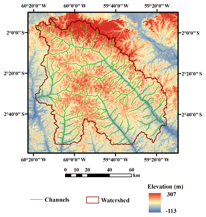
Figure 1Two-dimensional map of the watershed used in this study, showing the elevation, channels, and watershed boundary. The study area extends from 1∘57′36′′ to 2∘56′00′′ S and from 59∘14′48′′ to 60∘20′0′′ W.
The modeling tool used in this study is the PAWS model (Shen and Phanikumar, 2010; Shen et al., 2014; Niu et al., 2017). The main reason for choosing PAWS as the pilot example of PBHMs is that, compared with other PBHMs, PAWS is a comprehensive and representative large-scale hydrological model that can be applied to large catchments and long-term frames by efficiently coupling both surface and subsurface hydrological processes (Shen and Phanikumar, 2010). The complexity and parameter dimensionality of PAWS are high enough to test and demonstrate our new global sensitivity analysis method. Furthermore, PAWS was previously applied to the studied watershed, and it was capable of simulating multiple key variables of hydrological states and fluxes at different spatiotemporal scales and presented good model performance validated by various ground and satellite observation data (Niu et al., 2017). This previous model application provides a solid basis for our uncertainty identification and sensitivity analysis study.
The details of the numerical implementation and the governing equations of PAWS can be found in Appendix A. Briefly, four flow domains are simulated in PAWS, including the stream channel, overland flow, vadose zone, and saturated groundwater. The structured grid-based finite-volume method is the main numerical scheme applied to discretize the governing equations of the various hydrologic components. PAWS also simulates two land surface subdomains, i.e., infiltration and evaporation, which are depicted in the ponding subdomain, while overland flow occurs in the surface flow subdomain. PAWS considers the horizontal interaction of both surface runoff and groundwater flow between model grids, which represents the actual hydrological processes and is often ignored by other regional and global hydrologic models. The 1-D diffusive wave equation is solved to simulate channel flow, and the 2-D version is used for overland flow. The “leakance” concept is applied to explicitly simulate the exchange between the channel and groundwater. PAWS has been coupled with the CLM (Shen et al., 2014), which calculates the surface energy balance and soil and plant carbon and nitrogen cycles. Canopy interception and ET demand (both transpiration and soil evaporation) are also computed in the CLM at each time step.
For the numerical model case in this study, a 1 km× 1 km grid is used for horizontal discretization, resulting in 118 × 122 grid cells for the study site. In this model, 20 vertical layers are defined to discretize the vadose zone, and for the fully saturated groundwater, there are two layers: the unconfined aquifer at the top and the confined aquifer at the bottom. In this study, the 90 m resolution NASA Shuttle Radar Topography Mission (SRTM) (US Geological Survey; http://eros.usgs.gov, last access: 27 July 2020) data are applied as DEM input, but for the channel network and watershed boundary delineation, the Advanced Spaceborne Thermal Emission and Reflection Radiometer (ASTER) provides the 30 m resolution Global Digital Elevation Model Version 2 (GDEM V2). CLM land surface data are applied as land-use and land-cover (LULC) inputs. Details regarding these data can be found in Niu et al. (2017). More information on the governing equations of PAWS can be found in Shen and Phanikumar (2010) and Niu et al. (2014).
2.2 Hierarchical sensitivity analysis method with subdivided parametric sensitivity
The essential concept of the hierarchical sensitivity analysis method involves categorizing and quantifying different complex uncertainties of certain model systems while considering their dependence relationships. Different uncertainty sources (or uncertain inputs) are placed in different layers of a hierarchical uncertainty framework, which is then integrated with the variance-based global sensitivity analysis method to form a new set of sensitivity indices to accurately quantify the importance of different uncertainty sources.

Figure 2The framework of the hierarchical sensitivity analysis developed for PAWS and applied to the central Amazon basin. The three uncertainty source types are placed into the appropriate hierarchical level according to their dependence relationships. The left part of this figure shows the sources of these uncertainties, and the right side shows the abbreviations and the structural relationships among the various uncertainties. The number of climate scenarios (CSs) in this study is six; the number of plausible numerical models under each climate scenario is three; and the number of parameter sets under each numerical model is 600. Notably, the parameter uncertainty sources are further divided into three parts: vadose zone parameters, groundwater parameters, and the overland flow parameter.
In this study, climate scenarios, different aquifer thicknesses, and parameters are treated as random uncertain inputs, and they represent the climate scenario uncertainty, model uncertainty, and parameter uncertainty, respectively. Notably, the thicknesses of aquifers here represent the model uncertainty because the different thicknesses of distinct types of aquifers lead to different conceptual hydrological models, and a similar concept (different thicknesses were used for two underground geological formations) for the model uncertainty was used in previous work (Dai et al., 2017a). Six model parameters are included in this test case, and they are divided into three groups. The first group includes vadose zone parameters (PRVDZ): soil saturated hydraulic conductivity, Ks (m d−1); the van Genuchten equation parameters α (m−1); and N (unitless) (van Genuchten, 1980). The second group is composed of groundwater parameters (PRGW): unconfined aquifer hydraulic conductivity, K1 (m d−1), and confined aquifer hydraulic conductivity, K2 (m d−1). The third group is the overland flow parameter (PROVN): the length of the flow path for runoff contribution to the overland flow domain, L (m). Here, we consider the van Genuchten parameters α and N, because the correlation between α and N can largely affect the soil water release and infiltration processes in the vadose zone (Pan et al., 2011). In the hierarchical uncertainty framework, all these uncertainties are placed into the proper levels based on their dependence relationships. The climate scenario uncertainty is at the top layer, and the model uncertainty and parameter uncertainty are at the middle and bottom layers, respectively (Fig. 2), which is because the climate scenarios (CSs) are the driving forces of the hydrological model system, and multiple models can be built under a single scenario. Similar to the model and parameters, each model can contain a different set of parameters (Meyer et al., 2007). According to the hierarchical sensitivity analysis method, the partial variances contributed by the climate scenario uncertainty, model uncertainty, and parameter uncertainty can be expressed as Eqs. (1)–(3), respectively (see Appendix B for more details).
where Δ is the model output, CS represents the set of alternative climate scenarios, NM represents the multiple plausible models with different aquifer thicknesses, and PR represents the multiple parameter sets under a certain model. The notations of “NM|CS” and “PR|NM,CS” indicate the hierarchical relationships that models are conditioned on climate scenarios and parameters are conditioned on models and climate scenarios. The term “Δ|NM,CS” indicates that the output is calculated using the parameter sets that are conditioned on climate scenarios and models.
The sensitivity indices for the climate scenarios SCS, models SNM, and parameters SPR are expressed as Eqs. (4)–(6), following the hierarchical sensitivity analysis method:
where V(Δ) is the total variance in the model output (Eq. B5). The above equations are directly derived based on the hierarchical sensitivity analysis method. Notably, the parameter sensitivity index in Eq. (6) includes the influence of all parameters. However, to explore the detailed parameter sensitivity, the total parameter uncertainty is further decomposed into three components, representing the uncertainties contributed from vadose zone parameters (PRVDZ), groundwater parameters (PRGW), and the overland flow parameter (PROVN). Using the variance decomposition method (Eq. B1), the partial variance in the parameters can be further decomposed as follows:
where the notation PR∼VDZ refers to other uncertain parameters excluding vadose zone parameters, which are groundwater parameters and the overland flow parameter. The first term of Eq. (7) on the right-hand side is the partial variance contributed by PRVDZ, and the second term represents the partial variance in the other parameters, which are groundwater parameters and the overland flow parameter. Note that Eq. (7) is decomposed based on the vadose zone parameters; when we decompose the partial variance in parameters based on the groundwater parameters or the overland flow parameter, the partial variance in the parameters can be further decomposed as Eqs. (8) and (9):
The first terms in Eqs. (8) and (9) represent the partial variances contributed by the groundwater and overland flow parameters, respectively. Then, we can define a new set of subdivided parameter sensitivity indices for PRVDZ, PRGW, and PROVN following the first-order sensitivity index definition (Eq. B2):
2.3 Sensitivity index estimation using the LHS and binning method
The hierarchical sensitivity analysis method proposed by Dai et al. (2017a) was sampled using the conventional Monte Carlo random sampling method, which is computationally expensive for the sensitivity analysis of large-scale PBHMs. In this study, the different parameters were simultaneously sampled by the LHS method (Zhang and Pinder, 2003; Kanso et al., 2006). Compared with the conventional Monte Carlo method, the LHS method can guarantee space filling and noncollapsing of parameter samples (Grosso et al., 2009; Crombecq et al., 2011; Husslage et al., 2011; Damblin et al., 2013; Ba et al., 2015; Qian, 2012), which means that the sampling points can be evenly distributed throughout the sampling region and that there are no two sampling points with the same value. Thus, LHS is a sampling method with higher sampling efficiency (Helton and Davis, 2003). The convergence rate of the conventional Monte Carlo method is , where N is the sample size (Caflisch, 1998). However, for a system where the parameters are simply distributed (e.g., uniformly distributed), the convergence rate of LHS can reach O(N−3) (Iman and Conover, 1980). The LHS method has been one popular sampling technique used to reduce computational cost.
For the function Y=f(X), the input vector X consists of k parameters (i.e., ). By using the LHS method, the range of Xi, can be divided into n nonoverlapping intervals with equal probabilities. The n values obtained from X1 are randomly paired with n values obtained from X2; these n paired values are then combined with those n values from X3. We repeat this process until the new n×k sample matrix A is developed. This sample matrix A can be used to calculate the sensitivity index for the model output. More details regarding LHS are described in previous studies (McKay et al., 1979; Owen, 1998; Helton and Davis, 2003).
Using the variance definition, the partial variance in V(PR) can be first expressed as follows:
After applying the formula of expectation and the LHS method, the terms V(PR), V(NM) and V(CS) can be expressed as follows:
where n and j represent the total sample number of LHS and the index of LHS samples, respectively, P(NMk|CSl) represents the prior weight of model NMk under climate scenario CSl with , and P(CSl) is the prior weights of different CS satisfying . The values of the weights for alternative models or CS could be selected using prior knowledge or objective criteria, e.g., posterior probabilities of the Bayesian theorem (Neumann, 2012; Schöniger et al., 2014).
To calculate the subdivided parametric sensitivity indices, i.e., the sensitivity indices for vadose zone parameters, groundwater parameters, and overland flow parameter, a binning method was implemented in this study. This binning method was designed to estimate the partial variance terms of subdivided parameter groups with paired LHS samples of parameters. Using the sensitivity index of vadose zone parameters as an example, the range of vadose zone parameters was divided into multiple equal bins, and the partial variance term was approximated by using the model outputs calculated by those parameter sample pairs that contain vadose zone parameters in the same bin (noted as ). Then, the partial variance term in Eq. (10) can be computed as follows:
The subscript represents the vadose zone parameters in the same bins under the fixed model and fixed climate scenario. The subscript PRGW, , NM, CS represents the change in the combination of PRGW and PROVN sets belonging to a specific PRVDZ bin under a fixed model and fixed climate scenario. The term , NM, CS represents the output under the fixed vadose zone parameter, subsurface stratigraphy model, and climate scenario. refers to the weights of different bins for PRVDZ under the fixed model and fixed climate scenario.
The procedures for calculating the subdivided parametric sensitivity indices for PRVDZ using the combined LHS and binning methods are listed as follows: (1) simulate Δ for all CSs, models, and parameter realizations; (2) divide the PRVDZ realizations into bins; and (3) calculate by replacing it with . After is calculated for each bin of PRVDZ, the partial variance for PRVDZ, i.e., the numerator of Eq. (10), can be expressed as follows:
where the symbol U refers to the number of combinations of PRGW and PROVN in bin , i.e., the size of the parameter set in bin , and the symbol u is the index for these combinations. w represents the index for the bins of vadose zone parameters, and W is the total number of bins. After applying the LHS sampling method and the same binning method, the partial variance for PRGW and PROVN can be estimated as follows:
The binning method is a rigorously derived mathematical technique designed to separate and estimate the partial variances contributed from different parameters of one LHS method sampled parameter set. Because the mathematical equations are general and rigorous, this method can be applied to any modeling case with LHS parameter samplings. However, when the samplings for different parameters are totally random and unrelated, such as the conventional Monte Carlo simulation, the binning method is not applicable. Using LHS and the binning method, the number of realizations is reduced to the size of the parameter sets obtained from the LHS method. Thus, the computation cost for estimating the subdivided parametric indices can be highly reduced. Dai et al. (2017b) confirmed a similar accuracy of 36 000 000 Monte Carlo realization results with 16 000 realizations when applying only the binning method for a synthetic example. The combination of the LHS method with the binning method makes it computationally affordable to analyze the detailed parametric sensitivity for such a large-scale complex hydrologic model.
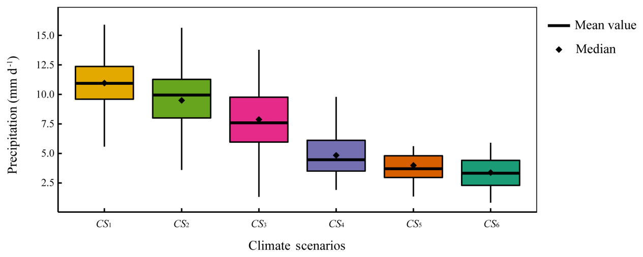
Figure 3We identified six CSs based on precipitation data for 1998–2013 from NASA's TRMM data (https://trmm.gsfc.nasa.gov/publications_dir/TRMM_Reentry_Risk_Assessment_FINAL_20150604.pdf). The first climate scenario (CS1) is the wettest one, and the sixth climate scenario (CS6) is the driest one.
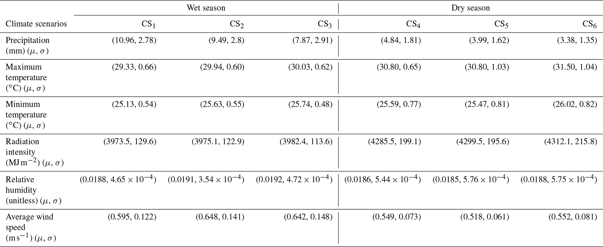
Table 1Statistical information for the daily data for the six CSs. Here, μ represents the mean value and σ represents the SD.
2.4 The generation of uncertain inputs
For the CS, we generated six typical and alternative scenarios based on NASA's Tropical Rainfall Measuring Mission (TRMM) data (https://trmm.gsfc.nasa.gov/publications_dir/TRMM_Reentry_Risk_Assessment_FINAL_20150604.pdf) and the default CLM CRU-NCEP (CRUNCEP) dataset (Piao et al., 2012) from 1998 to 2013. We considered five climate variables: daily precipitation, temperature, solar radiation, humidity, and wind speed. The precipitation data were obtained from TRMM, while the temperature, solar radiation, humidity, and wind speed data are based on the CRUNCEP, because the model fails to capture the peak stream discharges using the CRUNCEP rainfall data (Niu et al., 2017). We first divided the annual climate dataset into dry and wet seasons according to the precipitation values (6 months for each season). Then, we sorted the wet and dry seasons according to their total precipitation values during the whole season. Next, we divided these wet and dry seasons into three different groups representing six climate scenarios from wet to dry (Fig. 3). The mean and SD of the values of the different climate variables (e.g., precipitation, maximum temperature) for each group were calculated using the daily data (Table 1). Finally, we generated random daily weather data for each climate scenario based on these mean and SD data using a normal distribution. The mean and SD for each climate scenario's daily data are listed in Table 1, and Fig. 3 displays a box plot of the precipitation data for the six climate scenarios (CS1–CS6).
For the model uncertainty, the research of Brunke et al. (2016) shows that the shallow bedrock depth or deep bedrock depth has a great influence on surface runoff and base flow in CLM. Therefore, in this study, we will consider the effects of different aquifer models. Niu et al. (2017) simulated an unconfined aquifer with 100 m depth and 200 m thickness for the confined aquifer. Considering that (1) the stratification of the soil and aquifer is relatively stable (and the thickness does not change much) (do Rosário et al., 2016), (2) there is a lack of actual measurements in this area to determine the stratification of unconfined aquifers and confined aquifers, and (3) according to Pelletier et al. (2016), the thickness of the unconfined aquifer in the central Amazon is larger than 50 m (and the depth of the bedrock is very deep), three aquifer models involving different thicknesses of the unconfined and confined aquifers were generated to investigate the sensitivity of the model outputs to aquifer thickness. These three aquifer models involving different thicknesses of the unconfined and confined aquifers are (1) 100 and 200 m (NM1), (2) 50 and 250 m (NM2), and (3) 250 and 50 m (NM3), respectively. These three models represent the situations of (i) similar thickness of the unconfined and confined aquifer, with medium bedrock depth; (ii) thick confined aquifer, with low bedrock depth; and (iii) thick unconfined aquifer, with large bedrock depth.
Table 2Six chosen parameters to be included in parameter uncertainty.
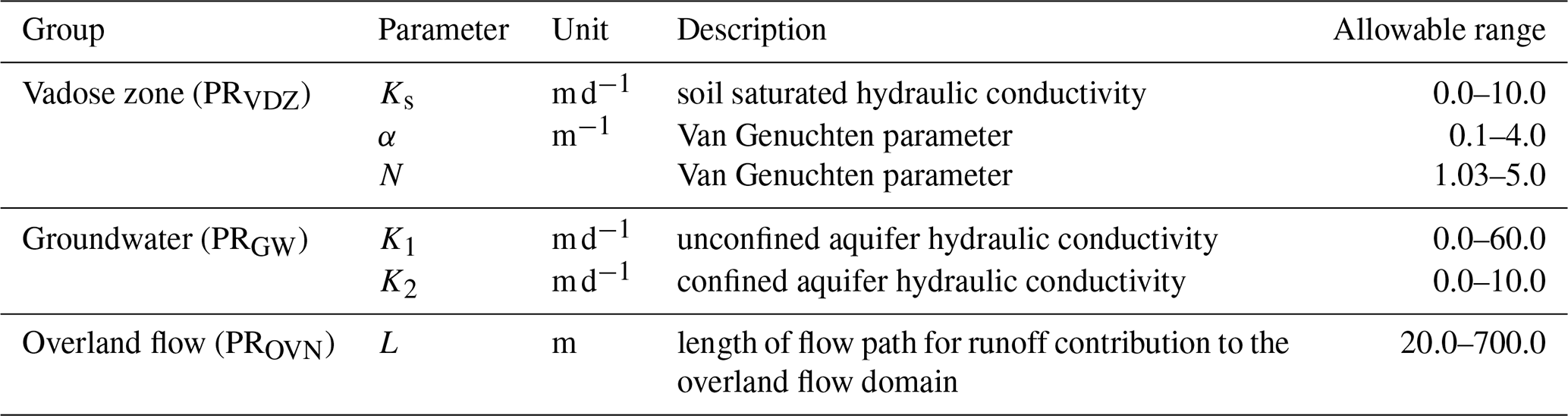
The six different model parameters were sampled by LHS within the feasible range (Table 2), and 600 samples of the parameter set were generated. The reasons for using 600 parameter samples in this study are because, first, based on the experiences of previous research cases (Emery et al., 2016; Dai et al., 2019), 600 is an adequate parameter sample size for this research considering the model domain and number of uncertain parameters and, second, considering the computational cost, 600 parameter samples is an appropriate sample size for this study. By combining model uncertainty and climate scenario uncertainty, there are 600 × 3 × 6 = 10 800 simulations in total. The pure simulation time without analyzing data is already very time consuming even when using the best high-performance computing (HPC) platform we have.
According to the study of Cuartas et al. (2012), the clay content in the northwestern part of Manaus is very high (65 %–90 %). Considering the difference in regional soil texture (Fisher et al., 2008; Teixeira et al., 2014), the allowable range of soil saturated conductivity, Ks, selected in this study is between 0 and 10 m d−1. The ranges of unconfined aquifer conductivity, K1, and confined aquifer conductivity, K2, are chosen as 0–10 and 0–60 m d−1, respectively. The results of the model calibration in Niu et al. (2017), which are related to the characteristics of the soil and groundwater layers in the watershed (Oleson et al., 2008; Christoffersen et al., 2014), are used to define the mean values of distributions used for these uncertain parameters. The soil saturated conductivity, Ks; unconfined aquifer conductivity, K1; and confined aquifer conductivity, K2, were assumed to follow lognormal distributions (log-N (1.6094, 0.42142), log-N (3.4012, 0.42142), and log-N (1.6094, 0.42142), respectively). The remaining three parameters (α, N, and L) were assumed to follow a uniform distribution: U (0.1, 4), U (1.03, 5), and U (20, 700). The allowable ranges of these six parameters are listed in Table 2.
From Sect. 3.1 to 3.4, we assumed that the different scenarios have equal probability. Moreover, three models under each climate scenario were also assumed to have equal weights, i.e., , and . However, the weights for models and scenarios may affect the output results. We investigated the variability in the results to the changing weights for NM1, CS1 (the wettest climate scenario), and CS6 (the driest climate scenario) in Sect. 3.5. This experiment is helpful for improving our understanding of sensitivity analysis results.
3.1 Model predictions
As mentioned in the above section, the total number of PAWS+CLM simulations considering all possible combinations of the three uncertain factors is 6 × 3 × 600 = 10 800, which represents six climate scenarios, three model conceptualizations of aquifer thickness, and 600 sampled parameter sets. We used the parallel computing technique for running these simulations through the HPC platform (13 cores of Xeon 2.8 GHz CPU). The average time spent on a single simulation was 2.8 min, and a total of 10 800 simulations were run for 3 weeks. The simulation time for all the simulations was 6 months (180 d, 4320 h), which is the length of the dry or wet season in the central Amazon region. The results given by PAWS were represented in two forms: (1) space-accumulative output values over the whole grid at each time step and (2) time-accumulative output values over the whole simulated period for each grid. In this study, the time step is 1 h. Figure 4 depicts the space-accumulative model predictions for the two outputs of interest, ET and QG, using different inputs of scenarios, models, and parameter sets. All prediction results are grouped into 24 groups based on local time, which represent 01:00 to 24:00 (all times are given in local time, LT, unless stated otherwise) throughout the day (Fig. 4). Each box in Fig. 4 describes the prediction results estimated using all the combinations of 600 parameter sets, three models, and six CSs at the same local times. Figure 4a shows that the ET predictions throughout a day have a time-varying pattern, and their values are significantly larger during the daytime and smaller at night. This pattern coincides with the physical fact that sunlight leads to higher temperature and more plant transpiration. The uncertainty of ET predictions during the daytime is also larger than that during the night. Figure 4b shows that the predictions of QG have no significant time-varying pattern throughout the day. However, the prediction results of ET and QG both demonstrate great variability or uncertainty for each time group. Further quantitative sensitivity analysis is necessary to identify the most important sources of uncertainty for these predictions.
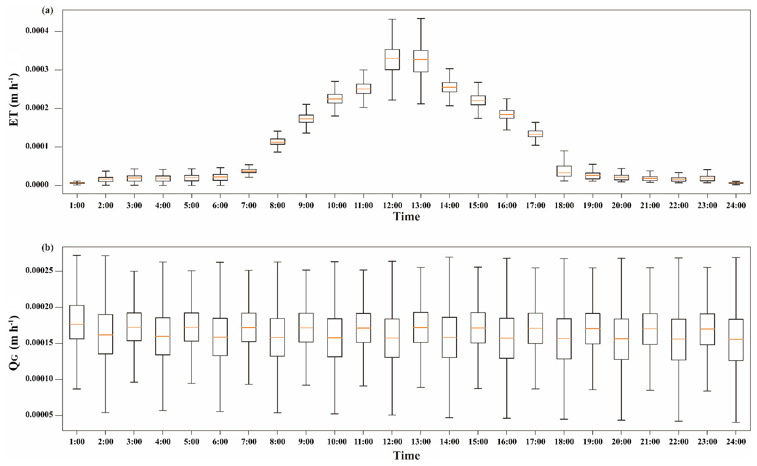
Figure 4The spatial-accumulative outputs for evapotranspiration (ET) (a) and groundwater contribution to stream flow (QG) (b) at all time steps and considering all three uncertainties. Each time step is divided into different groups based on local time. Different groups represent different hours of the day.
3.2 Sensitivity indices for evapotranspiration
First, we calculated the sensitivity indices for the space-accumulative ET over the whole watershed at all time steps using Eqs. (4)–(6). Figure 5a shows the sensitivity indices for the whole simulation period of 4320 time steps. All the sensitivity indices fluctuate strongly with time, except for the sensitivity indices of the models. The sensitivity indices for the models (SNM) are always close to zero at every time step, indicating that aquifer thickness has little influence on space-accumulative ET. Figure 5b–g plot the sensitivity indices across six periods, exhibiting the details at each time step. Every period lasts for 3 d. The patterns of the sensitivity indices have a daily cycle, but specific values of the sensitivity indices at the same wall-clock time on different days are distinguished. Figure 5 indicates that the sensitivity to various factors is strongly time dependent. Notably, at 12:00–13:00, the CSs are always the most important factors affecting the sensitivity of ET (Fig. 5b–g), which may be because ET is directly influenced by solar radiation values, and the radiation forcing used in this study reaches its maximum value at approximately 12:00. Therefore, the CSs dominate the uncertainties at 12:00–13:00. Another finding is that at 24:00–01:00 the sensitivity indices for the parameters (SPR) show absolute dominance, but the sensitivity indices for the climate scenarios (SCS) are decreased. A possible explanation for this result might be that precipitation and radiation forcing all decrease to zero during this period, leading to a decrease in the sensitivity indices for the climate scenarios (SCS). In contrast, the importance of parameters is greatly increased. Six time points (simulation times are 1428, 1440, 2868, 2880, 4308, and 4320 h) were chosen as examples to show the specific sensitivity indices (Fig. 6). Simulation times of 1428, 2868, and 4320 h belonged to different days, but all corresponded to 12:00 LT. At these time points, the climate scenario uncertainty (SCS) is the most important contributor to the total ET prediction uncertainty, accounting for 54 %–77 % of the total uncertainty, and parameters (SPR) contribute the second most to uncertainty. However, at different time points (1440, 2880, and 4320 h, corresponding to 24:00 LT), the parameters are the dominant uncertainty contributor, with SPR ranging from 89 % to 92 %.
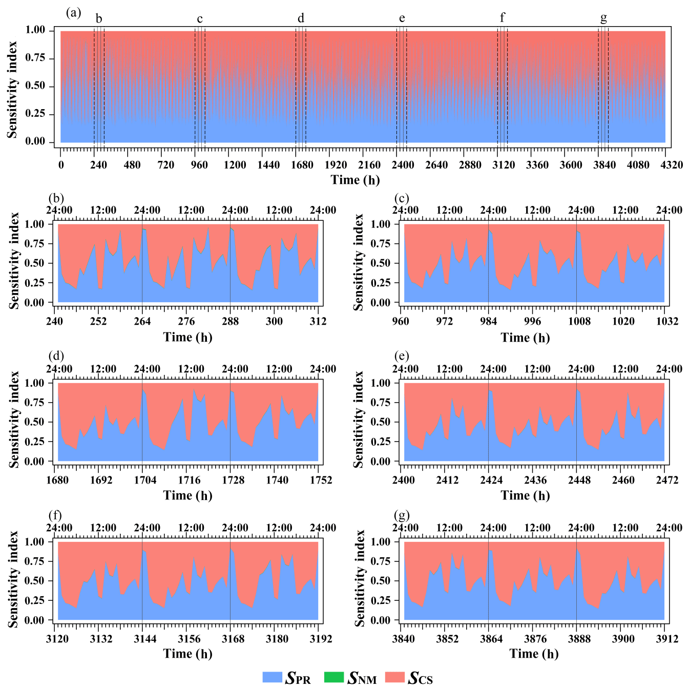
Figure 5Estimated sensitivities for the spatially averaged evapotranspiration (ET) at whole time steps (a). We chose six periods at 3 d intervals to display the sensitivity index values in detail. The bottom six figures exhibit the sensitivity index results for 241–312 h (b), 961–1032 h (c), 1681–1752 h (d), 2401–2472 h (e), 3121–3192 h (f), and 3841–3912 h (g). SPR is the sensitivity index for parameters. SNM is the sensitivity index for models and represents the influence of aquifer thickness. The SCS is the sensitivity index for climate scenarios. The bottom x axis of (b–g) represents the simulated time steps, and the upper x axis of (b–g) represents the local time.
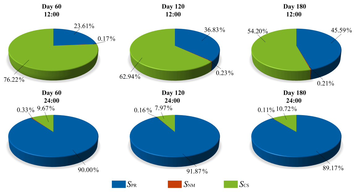
Figure 6Estimated sensitivities for the spatially averaged evapotranspiration (ET) at six time points (simulation times are 1428 h (Day 60, 12:00), 1440 h (Day 60, 24:00), 2868 h (Day 120, 12:00), 2880 h (Day 120, 24:00), 4308 h (Day 180, 12:00), and 4320 h (Day 180, 24:00)). SPR is the sensitivity index for the parameters. SNM is the sensitivity index for the numerical models, and SCS is the sensitivity index for the climate scenarios.
We also calculated the sensitivity indices for every grid cell within the model domain using the time-accumulative ET predictions over all simulation periods (4320 h). Figure 7 shows the spatial variability in the sensitivity indices for the temporal mean ET predictions. The maps demonstrate that for most grids, parameters are the most important uncertainty contributor to ET predictions (SPR > 0.50), and CS are the second most important contributor to uncertainty. However, for stream grid cells, the importance of aquifer thicknesses increases. Therefore, the parameters and aquifer thicknesses are both important. Here, aquifer thicknesses refer to the average aquifer thickness for the whole watershed. The increase in the model sensitivity indices indicates that the structure of the aquifer significantly affects the baseflow and then influences the river evaporation predictions. Figure 7 shows that the parameter uncertainty within the overall watershed is important for ET, and for river evaporation, the aquifer thicknesses are also important.
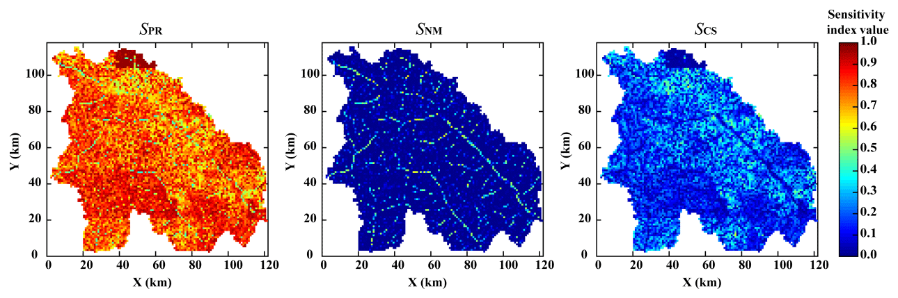
Figure 7Maps of parametric (SPR), numerical model (SNM), and climate scenario (SCS) sensitivity index values for time-averaged evapotranspiration (ET) predictions.
3.3 Sensitivity indices for groundwater contribution to streamflow
Groundwater has been demonstrated to be crucial for soil moisture in the Amazon region by previous research (Miguez-Macho and Fan, 2012b). Meanwhile, it also exerts a significant buffering effect on maintaining evapotranspiration during dry seasons (Miguez-Macho and Fan, 2012a; Pokhrel et al., 2014). The model PAWS uses the output of QG to quantify the variation in groundwater volumes and measure the interaction process between groundwater and rivers. It is essential to implement the sensitivity analysis to investigate which factor is most influential on this groundwater exchange process. The same sensitivity analysis procedures were also conducted for the model predictions of QG.
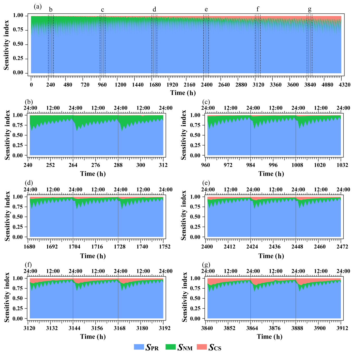
Figure 8Estimated sensitivities for the spatially averaged groundwater contribution to stream flow (QG) at whole time steps (a). We chose six periods at 3 d intervals to display the sensitivity index values in detail. The bottom six figures exhibit the sensitivity index results for 241–312 h (b), 961–1032 h (c), 1681–1752 h (d), 2401–2472 h (e), 3121–3192 h (f), and 3841–3912 h (g). SPR is the sensitivity index for parameters. SNM is the sensitivity index for models and represents the influence of aquifer thickness. The SCS is the sensitivity index for climate scenarios. The bottom x axis of (b–g) represents the simulated time steps, and the upper x axis of (b–g) represents the local time.
Figure 8a shows the sensitivity indices for the whole simulation period of 4320 time steps for QG predictions. This figure indicates that regardless of the time steps, parameters are always the dominant contributor to the total QG prediction uncertainty. This result may be explained by the fact that soil parameters strongly affect the soil water redistribution process, including infiltration into groundwater. We selected the same period as Fig. 5b–g to display the more detailed results for QG predictions in Fig. 8b–g. As shown in these figures, the sensitivity indices of the models (SNM) and climate scenarios (SCS) reach peak values at approximately 01:00. In terms of SCS, this may be because the exchange between groundwater and river flow occurs hours later than the rainfall process, and the amount of water during the exchange process always reaches its peak at night, at approximately 01:00. The SNM might be because the thickness of aquifers will greatly influence the water redistribution process in the aquifer. Another pattern demonstrated in Fig. 8 is that the values of SCS generally increase with time. This trend may be caused by the seasonality effect of CS or the long-term cumulative influence of CS on the groundwater flow.

Figure 9Maps of parametric sensitivity indices (SPR), numerical model sensitivity indices (SNM), and climate scenario sensitivity indices (SCS) for the time-averaged groundwater contribution to stream flow (QG) predictions.
Because groundwater exchange with stream flow occurs only at grid cells along the streams, the sensitivity indices only have valid values in those stream grid cells (Fig. 9). Our results indicate that considering most grid cells, the parameters are the most important contributor to the uncertainty of time-accumulative QG predictions, and the second most important factor is aquifer thickness. However, if we divide the grid cells into groundwater and stem river grid cells based on their location relative to the river and aquifer type, the sensitivity analysis results are totally different in these two types of grid cells. The model parameter uncertainty is usually the most important in stem river grid cells; in contrast, the aquifer thicknesses contribute the largest portion of the uncertainty in groundwater grid cells. This pattern of results may be caused by the unconfined aquifer and river being unconnected in the stem river grid cells, and there is an unsaturated zone between two of them. Therefore, the soil parameters affect QG predictions in stem river grid cells. Moreover, the groundwater table is relatively high, and the groundwater is directly connected with rivers in the groundwater grid cells. Thus, the aquifer thicknesses are more important under this condition.
3.4 Sensitivity indices for subdivided parameters
Based on the sensitivity analysis for ET and QG predictions, the results show that parameters are important uncertain inputs for both the space-accumulative and time-accumulative uncertainties. In this study, we used Eqs. (10)–(12) to further calculate the subdivided parametric sensitivity indices, which can provide a more detailed sensitivity analysis for model simulation. Through this investigation, the parametric sensitivity was subdivided into three groups: (1) the sensitivity for vadose zone parameters (), (2) the sensitivity for groundwater parameters (), and (3) the sensitivity for the overland flow parameter (). Using the binning method, we calculated the space-accumulative and time-accumulative subdivided parametric sensitivity indices for ET and QG. We plotted frequency histograms of the subdivided parametric sensitivity indices over 4320 h in Fig. 10.
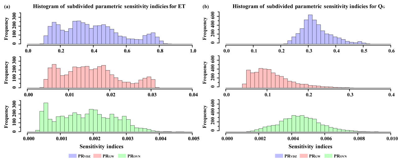
Figure 10Frequency histograms of subdivided parametric sensitivity indices for spatially averaged results over all 4320 time steps. The results for evapotranspiration (ET) as our output are depicted in (a), and the results for groundwater contribution to stream flow (QG) as our output are depicted in (b). PRVDZ represents the vadose zone parameters. PRGW represents the groundwater parameters. PROVN represents the overland flow parameter.
Figure 10a depicts the results for ET. The value of is concentrated in the range of 0.1–0.9, and is concentrated in the range of 0.003–0.032. The value of is so small that the influence of the overland flow parameter can be ignored. This indicates that vadose zone parameters (PRVDZ) dominate the total parametric uncertainties for ET. Figure 10b shows the frequency histogram of space-accumulative subdivided parametric sensitivity results for QG; is still concentrated in the larger number range (0.2–0.53), and the value of changes from 0.04 to 0.3. The number of is also the lowest, indicating that the overland flow parameter has little effect on QG. The order of importance of the uncertain inputs is the same for both ET and QG predictions. However, it is significantly different from ET in that although PRGW is the second most important parameter group, the value of in the QG results is an order of magnitude higher than that in the ET results. In the QG results, the range of is concentrated in the range of 0.05–0.2, while in the ET results, the value of is concentrated in the range of 0.003–0.032.
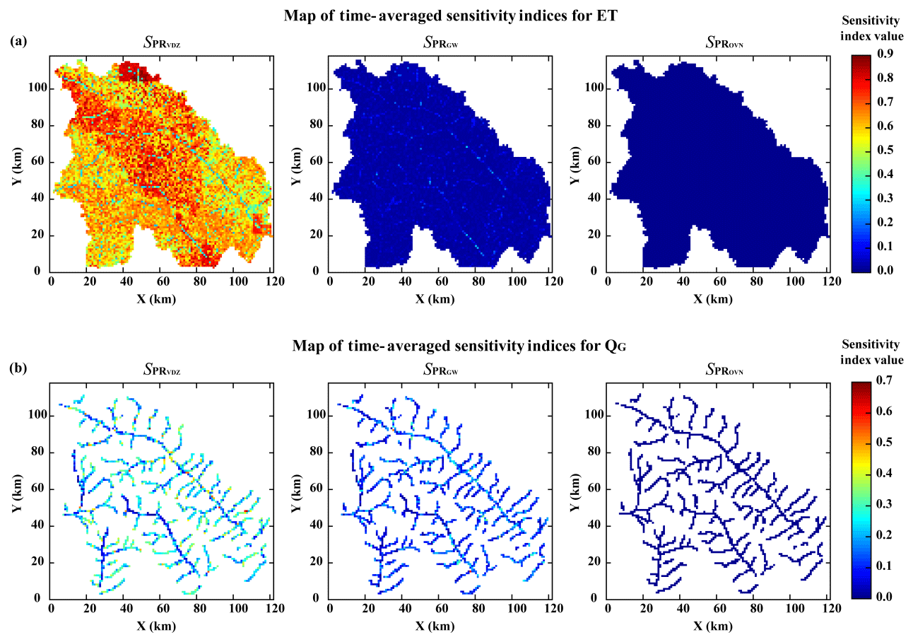
Figure 11Maps of vadose zone parameter sensitivity indices (), groundwater parameter sensitivity indices (), and overland flow parameter sensitivity indices () for time-averaged evapotranspiration (ET) (a) and groundwater contribution to stream flow (QG) (b) predictions.
We plotted the time-accumulative subdivided parametric sensitivity indices for ET in Fig. 11a and for QG in Fig. 11b. Considering ET as our output, for most grids, the vadose zone parameters are the most important contributor to parametric uncertainties. Compared with that on other grids, the influence of groundwater parameters on the river grids is more significant (Fig. 11a). For the QG results, the vadose zone parameters generally dominate the parametric sensitivities for most grids (Fig. 11b). However, if considering different types of grid cells, we find that the vadose zone parameters mainly affect the stem river grid cells and have a relatively small influence on the groundwater grid cells. This pattern coincides with our hypotheses that there is an unsaturated zone between the stem rivers and groundwater. More detailed sensitivity indices for all six parameters are demonstrated in Appendix C.
3.5 Effects of prior weights on sensitivity indices
In this section, we changed the prior weights of the CS and numerical models to investigate their influences on the space-accumulative sensitivity indices. Because the number of space-accumulative results for ET and QG is too large to be well exhibited, we chose one time step (4308 h, 12:00 wall-clock time) to show the trend. We randomly changed the values of the weights for NM1 (the thickness of the unconfined aquifer is 50 m and that of the confined aquifer is 250 m), CS1 (the wettest climate scenario), and CS6 (the driest climate scenario) to between 0 and 1. If the weight for NM1, CS1, or CS6 is p, then the weight of the remaining climate scenarios or models will be assumed to be , where n is the number of the remaining climate scenarios or models. Figure 12a indicates that when we consider ET as our output, with the increase in the prior weight of NM1, the uncertainty of the CS will decrease to 50 %, while the uncertainty of the parameters will increase to 50 %. Both parameters and CSs have important effects on ET. Different from the results for ET, with the increase in the prior weights of NM1, the sensitivity index of the numerical models for QG decreases to 0 (because only one model exists under this condition), and the scenario uncertainty changes only slightly. Moreover, the uncertainty of parameters always dominates the total uncertainty for QG (Fig. 12b) regardless of the prior weight value. In general, the different prior weight values for the numerical models only slightly change the sensitivity analysis results.
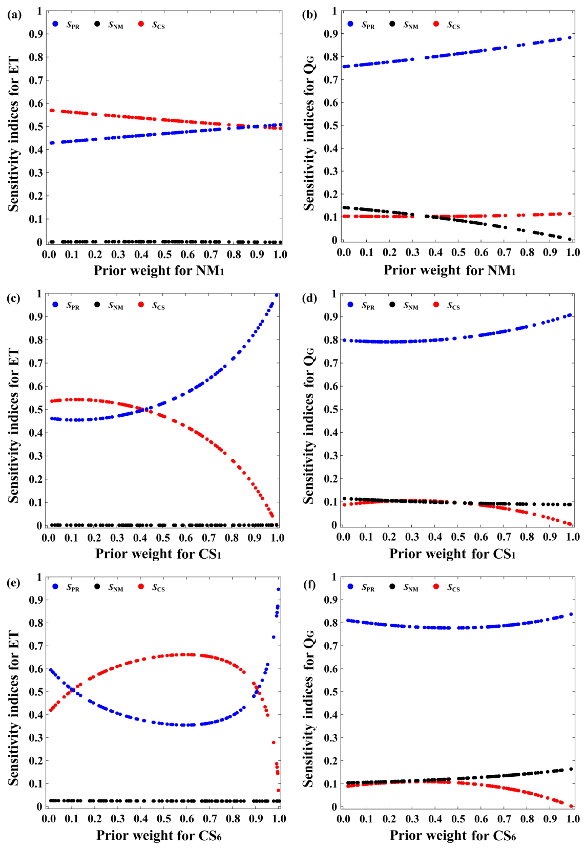
Figure 12Patterns of SPR, SNM, and SCS for space-averaged evapotranspiration (ET) and space-averaged groundwater contribution to stream flow (QG) with changes in the prior weights of numerical model NM1, climate scenario CS1, and climate scenario CS6 at the time step of 4308 h (at 12:00).
Figure 12c–f exhibits the influences of prior weights for the wettest and driest CS on ET. These figures first demonstrate that changing the values of the prior weights of CS1 and CS6 has larger impacts on ET predictions than on QG predictions. This pattern coincides with the fact that the parameter uncertainty dominates the total predictive uncertainty of QG and that the scenario uncertainty is relatively small. Therefore, the selection of prior weight values for the scenarios does not have a significant effect on the sensitivity analysis results for the QG predictions, and the parameter sensitivity index is always the largest (Fig. 12d and f). For the sensitivity analysis results pertaining to ET predictions, changing the values of the weights for CS1 and CS6 has different effects. The sensitivity index values of the climate scenarios for ET predictions monotonically decrease, while the importance of parameters continues to increase as the prior weight of CS1 is larger than 40 %, which reflects that when the probability of extreme humid seasons in the Amazon is greater than 40 %, the importance of parameters takes precedence over the importance of climate scenarios for ET. However, the value of SCS for ET predictions first increases when the prior weight of CS6 approaches 10 % and then decreases after the prior weight of CS6 approaches 90 %, and SPR shows the opposite trend (Fig. 12e). This shows that when the probability of occurrence of extreme dry seasons is between 10 % and 90 %, the climate scenario is always the most important uncertain input unless the occurrence probability of the extreme dry season is greater than 90 %.
3.6 Discussion
The results from this case study exhibit the importance of parameters, especially the vadose zone parameters, for ET and QG predictions. Furthermore, according to the space-accumulative results, the climate scenario is also an important uncertainty source for ET predictions, especially at 12:00. Meanwhile, the thickness of the aquifer has a nonignorable influence on the QG predictions on the groundwater grid cells. Moreover, according to the results of adjusting the climate scenario and model weights, the change in model (aquifer thickness) weights only has a small impact on the importance of different uncertainties. When the probability of occurrence of the extreme humid season is high, the importance of the parameters increases significantly. However, when the probability of occurrence of the extreme dry season is high, the main factors affecting ET predation are still the climate scenario unless the probability of occurrence of CS is greater than 90 %. Although these patterns of sensitivity analysis results may not be universally correct, they can still provide useful insights for other modelers with similar cases and models.
In addition to the specific results, we also have some new insights into the general patterns of sensitivity analysis for the PBHMs provided by this pilot case. For instance, first, the ranks of importance of uncertain inputs are totally different for different model outputs; e.g., CSs have a large impact on ET predictions but a small impact on QG predictions. There is no one set of results that are valid for all different model outputs. Second, the sensitivity analysis results of ET and QG predictions show that the uncertainty has high temporal and spatial variability, which reflects that for very complex hydrological models, such as PBHMs, it is incorrect to generalize the sensitivity analysis results of a grid or a time step to the entire watershed or the entire simulation cycle. Third, it is necessary to implement such a comprehensive global sensitivity analysis method that considers more than parametric uncertainty for the large-scale PBHMs since the sensitivity analysis results showed that other sources of uncertainty (e.g., climate scenario and model uncertainties) are essential as well for model predictions. Finally, evaluating the sensitivity of the parameters in detail is essential for PBHMs. For such a complex surface–subsurface coupling model, the new sensitivity analysis method can efficiently identify the uncertain inputs that have the greatest impact on the model outputs. This process can greatly improve our understanding of the complex model system and save time that is normally spent calibrating the model.
This research presented an improved hierarchical sensitivity analysis method for comprehensive global sensitivity analysis of large-scale complex PBHMs. Developed based on the previous hierarchical framework of Dai et al. (2017a), this new methodology can simultaneously consider various types of uncertainty sources and estimate the importance of different processes involved in the modeling work. A new set of sensitivity indices of subdivided parameters was defined to quantify the importance of processes that only involve partial parameters. The highly efficient sampling algorithm of the LHS and binning method were implemented for the estimation of sensitivity indices to reduce computational cost. For evaluation and demonstration purposes, we implemented the new sensitivity analysis method into a real-world case of large-scale complex PBHM (PAWS), which was applied to a large Amazon catchment. Three common groups of uncertainty sources or uncertain inputs were considered in this study, including six CSs, three plausible aquifer models, and six uncertain parameters (i.e., soil saturated conductivity, van Genuchten α and N, unconfined aquifer conductivity, confined aquifer conductivity, and the length of the flow path for runoff contribution to the overland flow domain). A new set of subdivided parametric sensitivity indices was defined for three groups of parameters (i.e., vadose zone, groundwater, and overland flow parameters).
The sensitivity analysis results in this study first demonstrate the necessity of implementing such a comprehensive global sensitivity analysis for PBHMs, because uncertainty sources other than parameters (e.g., CS and models) are also important for model predictions. Furthermore, the values of model weights have a small impact on the sensitivity analysis results, but the selections of weights for extreme CSs may change the ranks of importance for uncertain inputs. Moreover, the sensitivity analysis results are both temporally and spatially dependent and have distinct patterns for different model outputs. Therefore, there is no single conclusion for all model outputs considering different times and locations. In general, the parameter uncertainty is important for both ET and QG predictions. Among all the parameters, the vadose zone parameters are the most important, and the parameter of overland flow is negligible. The CSs are also important uncertainties for ET predictions, especially at 12:00. Along the river grid cells, the thickness of the aquifer has a significant influence on both ET and QG predictions. Although the patterns of sensitivity analysis results found in this study may not be universally valid, they can still provide useful insights for modelers with similar problems. For instance, we can suggest that when modelers apply sophisticated hydrological simulators, such as PAWS, they should pay more attention to the values of weather variables at approximately 12:00 (the daily peak values) and focus more on estimating the thicknesses of groundwater aquifers near rivers and adjusting the vadose zone parameters.
Through this pilot example of comprehensive global sensitivity analysis, this study proves that using the new improved hierarchical sensitivity analysis method is a computationally affordable and useful way to identify the most important uncertain inputs for large-scale complex PBHMs. The sensitivity analysis results can provide key information on uncertainty sources for modelers and greatly improve the model calibration and uncertainty analysis processes. The proposed method is mathematically rigorous and general and can be applied to extensive large-scale hydrological or environmental models with different sources of uncertainty.
The governing equations of PAWS are presented in detail in Shen and Phanikumar (2010) and Shen et al. (2013). Here, we will mainly introduce the equations describing the processes involved in this article.
In PAWS, the soil moisture in the vadose zone is calculated according to the Richards equation. The vertical movement of fluid between saturated and unsaturated soil is calculated based on the mixed form of the Richards equation (Celia et al., 1990; van Dam and Feddes, 2000):
where h represents the soil water pressure head, z is the elevation (positive upward), K(h) represents the soil unsaturated conductivity, and W(h) is the source or sink term, including the influence of evaporation, root extraction, and lateral flow. The differential water capacity can be described as , where h is the soil pressure head and θ is the water content. The pressure head, h, is related to the unsaturated hydraulic conductivity, K(h). According to the Mualem–van Genuchten formula (Mualem, 1976; van Genuchten, 1980), the soil saturated hydraulic conductivity, Ks, and van Genuchten parameters α and N will influence the unsaturated conductivity, K(h):
where S is the relative saturation, θs is the saturated water content, θr is the residual water content, N is related to the pore size distribution, α indicates the reciprocal of air suction, and λ is a parameter measuring pore connectivity.
The aquifers in PAWS are depicted as a series of 2-D layers (Shen et al., 2014). In each layer, the 2-D groundwater equation is used to describe the water movement:
where S is the storability and T is the transmissivity of the aquifer; T=Kb, where K is the aquifer conductivity and b is the saturated thickness of the aquifer; H is the aquifer hydraulic head; R is recharge or discharge; W is the source and sink term; and Dp is percolation into deeper aquifers.
PAWS applies one-dimensional diffusive wave equations to portray the channel flow model (Shen and Phanikumar, 2010; Shen et al., 2014). After calculating the channel flow, the exchange between groundwater and channel flow (QG) is immediately computed. The calculation of QG is based on the leakance concept (Shen and Phanikumar, 2010):
where is the river level calculated from the channel flow model, Kr is the riverbed conductivity, Zb is the elevation of the riverbed, ΔZb is the thickness of the riverbed, and H∗ is the groundwater table. Note that H∗ can also be described as Eq. (A5). By solving these two equations together, we can obtain H∗ and . Then, the value of QG can be calculated as follows (Shen and Phanikumar, 2010):
where w is the wetted perimeter. If the river width is greater than 10 m, w can be approximated as the river width.
PAWS retains its own flow scheme, but the surface processes use the CLM 4.0 model, which enables the simulation of detailed surface processes, such as surface heat flux, water vapor flux, surface radiation balance, crop growth, and plant photosynthesis. The calculation of ET demand is performed in the CLM model based on the climate data, and then, ET demand will be transferred to PAWS as a source term for the vadose zone. More details about the calculation of ET (both evaporation and transpiration information can be found in the technical note of CLM 4.0, http://www.cesm.ucar.edu/models/cesm1.1/clm/CLM4_Tech_Note.pdf, last access: 27 July 2020). The coupling with the CLM makes PAWS a more comprehensive and robust surface–subsurface hydrological model.
For the model, , where Δ is the model output and is a group of uncertainty inputs; using the law of total variance, the total variance in Δ can be decomposed as follows (Dai et al., 2017a):
where the first term of partial variance on the right-hand side is the within-Xi partial variance and represents the variance contribution by Xi, and X∼i represents all the inputs except Xi. The second term on the right-hand side represents the variance contributed by the model inputs excluding Xi as well as the interactions of all the inputs. Based on the definition of the first-order sensitivity index (Saltelli and Sobol, 1995),
The percentage of uncertainty contributed by input Xi can be accurately quantified.
For the hierarchical framework in Fig. 2, the variance-based sensitivity analysis method enables decomposition of the total variance into individual contributors as follows:
The first term of partial variance on the right-hand side of this equation represents the variance caused by multiple CSs. The second term on the right-hand side is the partial variance caused by other uncertain inputs and can be further decomposed as follows:
where the first partial variance term on the right-hand side of this equation represents the uncertainty contributed by multiple plausible models. The second term represents the within-model partial variance caused by the uncertain parameters. By substituting Eq. (B4) back into Eq. (B3), we can obtain the following equation:
The three terms on the right-hand side of Eq. (B5) represent the partial variances contributed by the parameters, models, and CSs, respectively. The equation indicates that the total variance can be decomposed into the variances contributed by the alternative climate scenarios, denoted by CS; plausible numerical models, denoted by NM; and uncertain parameters, denoted by PR. Then, following the first-order sensitivity index definition (Eq. B2), the hierarchical sensitivity analysis method defines the indices for PR, NM, and CS, respectively, as shown in Eqs. (4)–(6).
To conduct a more comprehensive analysis of all parameters and to compare the impact of two aquifers on QG, we estimated the sensitivity indices of the six parameters according to Eq. (C1). The difference between this equation and the previous ones is that Eq. (C1) no longer groups the parameters, and it calculates the sensitivity indices individually for six parameters.
In this equation, θ refers to one of the six parameters, i.e., Ks, α, N, K1, K2, or L. The subscript “θ|NM,CS” represents the change in one parameter under a fixed model and a climate scenario. The subscript “” refers to the other five uncertain parameter inputs excluding θ parameter. The term “” represents the output under the fixed θ, model, and climate scenario.
The spatial distribution of the sensitivity indices of six parameters for QG is shown in Fig. C1. According to Fig. C1, the importance of the van Genuchten parameter N in the stem grid cells is significant. The conductivity of unconfined aquifer K1 has a certain impact on QG in most river grid cells. Additionally, it can also be seen from Fig. C1 that for most grids the influence of K1 is greater than K2, which implies that the unconfined aquifer has a greater influence on baseflow.
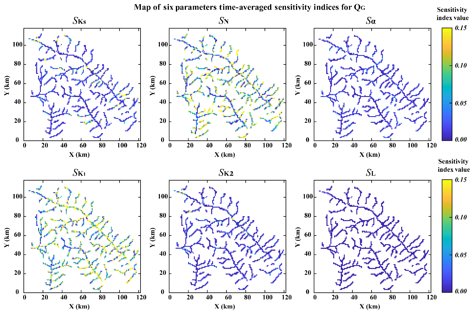
Figure C1Maps of six parameter sensitivity indices for groundwater contribution to stream flow (QG) predictions.
The weather dataset is available from the default CLM CRU–NCEP (CRUNCEP) dataset and https://disc.gsfc.nasa.gov/mirador-guide?project=TRMM&tree=project (NASA Orbital Debris Program Office, 2015). The sensitivity data and the source code used for analyzing the sensitivity data in this study are freely available upon request.
HD and JN were involved in the project conceptualization and formulating the methodology. HL performed the experiments and analyzed and visualized the data with guidance from HD and JN. HL prepared the original paper, with contributions from HD, JN, HQ, and WR. DG, BXH, MY, JZ, CW, and XC helped shape the initial ideas for this research.
The authors declare that they have no conflict of interest.
This work was supported by the National Natural Science Foundation of China (grant no. 41807182), Western Light – western region leading scientists supporting project, Chinese Academy of Sciences (2018-XBYJRC-002).
This research has been supported by the National Natural Science Foundation of China (grant no. 41807182) and the Western Light – western region leading scientists supporting project, Chinese Academy of Sciences (grant no. 2018-XBYJRC-002).
This paper was edited by Alberto Guadagnini and reviewed by three anonymous referees.
Ba, S., Myers, W. R., and Brenneman, W. A.: Optimal sliced Latin hypercube designs, Technometrics, 57, 479–487, 2015.
Baroni, G. and Tarantola, S.: A General Probabilistic Framework for uncertainty and global sensitivity analysis of deterministic models: a hydrological case study, Environ. Modell. Softw., 51, 26–34, https://doi.org/10.1016/j.envsoft.2013.09.022, 2014.
Beven, K.: Towards an alternative blueprint for a physically based digitally simulated hydrologic response modelling system, Hydrol. Process., 16, 189–206, https://doi.org/10.1002/hyp.343, 2002.
Bixio, A., Gambolati, G., Paniconi, C., Putti, M., Shestopalov, V., Bublias, V., Bohuslavsky, A., Kasteltseva, N., and Rudenko, Y.: Modeling groundwater-surface water interactions including effects of morphogenetic depressions in the Chernobyl exclusion zone, Environ. Geol., 42, 162–177, https://doi.org/10.1007/s00254-001-0486-7, 2002.
Brunke, M. A., Broxton, P., Pelletier, J., Gochis, D., Hazenberg, P., Lawrence, D. M., Leung, L. R., Niu, G.-Y., Troch, P. A., and Zeng, X.: Implementing and evaluating variable soil thickness in the community land model, Version 4.5 (CLM4.5), J. Climate, 29, 3441–3461, https://doi.org/10.1175/jcli-d-15-0307.1, 2016.
Caflisch, R. E.: Monte carlo and quasi-monte carlo methods, Acta numer., 1998, 1–49, 1998.
Celia, M. A., Bouloutas, E. T., and Zarba, R. L.: A general mass-conservative numerical solution for the unsaturated flow equation, Water Resour. Res., 26, 1483–1496, https://doi.org/10.1029/WR026i007p01483, 1990.
Chávarri, E., Crave, A., Bonnet, M.-P., Mejía, A., Santos Da Silva, J., and Guyot, J. L.: Hydrodynamic modelling of the Amazon River: factors of uncertainty, J. S. Am. Earth Sci., 44, 94–103, https://doi.org/10.1016/j.jsames.2012.10.010, 2013.
Christoffersen, B. O., Restrepo-Coupe, N., Arain, M. A., Baker, I. T., Cestaro, B. P., Ciais, P., Fisher, J. B., Galbraith, D., Guan, X., Gulden, L., van den Hurk, B., Ichii, K., Imbuzeiro, H., Jain, A., Levine, N., Miguez-Macho, G., Poulter, B., Roberti, D. R., Sakaguchi, K., Sahoo, A., Schaefer, K., Shi, M., Verbeeck, H., Yang, Z.-L., Araújo, A. C., Kruijt, B., Manzi, A. O., da Rocha, H. R., von Randow, C., Muza, M. N., Borak, J., Costa, M. H., Gonçalves de Gonçalves, L. G., Zeng, X., and Saleska, S. R.: Mechanisms of water supply and vegetation demand govern the seasonality and magnitude of evapotranspiration in Amazonia and Cerrado, Agr. Forest Meteorol., 191, 33–50, https://doi.org/10.1016/j.agrformet.2014.02.008, 2014.
Crombecq, K., Laermans, E., and Dhaene, T.: Efficient space-filling and non-collapsing sequential design strategies for simulation-based modeling, Eur. J. Oper. Res., 214, 683–696, 2011.
Cuartas, L. A., Tomasella, J., Nobre, A. D., Nobre, C. A., Hodnett, M. G., Waterloo, M. J., de Oliveira, S. M., von Randow, R. D. C., Trancoso, R., and Ferreira, M.: Distributed hydrological modeling of a micro-scale rainforest watershed in Amazonia: Model evaluation and advances in calibration using the new HAND terrain model, J. Hydrol., 462–463, 15–27, https://doi.org/10.1016/j.jhydrol.2011.12.047, 2012.
Dai, H. and Ye, M.: Variance-based global sensitivity analysis for multiple scenarios and models with implementation using sparse grid collocation, J. Hydrol., 528, 286–300, https://doi.org/10.1016/j.jhydrol.2015.06.034, 2015.
Dai, H., Chen, X., Ye, M., Song, X., and Zachara, J. M.: A geostatistics-informed hierarchical sensitivity analysis method for complex groundwater flow and transport modeling, Water Resour. Res., 53, 4327–4343, https://doi.org/10.1002/2016wr019756, 2017a.
Dai, H., Ye, M., Walker, A. P., and Chen, X.: A new process sensitivity index to identify important system processes under process model and parametric uncertainty, Water Resour. Res., 53, 3476–3490, https://doi.org/10.1002/2016wr019715, 2017b.
Dai, H., Chen, X., Ye, M., Song, X., Hammond, G., Hu, B., and Zachara, J. M.: Using Bayesian networks for sensitivity analysis of complex biogeochemical models, Water Resour. Res., 55, 3541–3555, 2019.
Damblin, G., Couplet, M., and Iooss, B.: Numerical studies of space-filling designs: optimization of Latin Hypercube Samples and subprojection properties, J. Simul, 7, 276–289, https://doi.org/10.1057/jos.2013.16, 2013.
de Paiva, R. C. D., Buarque, D. C., Collischonn, W., Bonnet, M.-P., Frappart, F., Calmant, S., and Bulhões Mendes, C. A.: Large-scale hydrologic and hydrodynamic modeling of the Amazon River basin, Water Resour. Res., 49, 1226–1243, https://doi.org/10.1002/wrcr.20067, 2013.
do Rosário, F. F., Custodio, E., and da Silva, G. C.: Hydrogeology of the Western Amazon Aquifer System (WAAS), J. S. Am. Earth Sci., 72, 375–386, https://doi.org/10.1016/j.jsames.2016.10.004, 2016.
Emery, C. M., Biancamaria, S., Boone, A., Garambois, P.-A., Ricci, S., Rochoux, M. C., and Decharme, B.: Temporal variance-based sensitivity analysis of the river-routing component of the large-scale hydrological model ISBA–TRIP: application on the Amazon Basin, J. Hydrometeorol., 17, 3007–3027, https://doi.org/10.1175/jhm-d-16-0050.1, 2016.
Fisher, R. A., Williams, M., de Lourdes Ruivo, M., de Costa, A. L., and Meir, P.: Evaluating climatic and soil water controls on evapotranspiration at two Amazonian rainforest sites, Agr. Forest Meteorol., 148, 850–861, https://doi.org/10.1016/j.agrformet.2007.12.001, 2008.
Freeze, R. A. and Harlan, R.: Blueprint for a physically-based, digitally-simulated hydrologic response model, J. Hydrol., 9, 237–258, 1969.
Gedeon, M. and Mallants, D.: Sensitivity analysis of a combined groundwater flow and solute transport model using local-grid refinement: a case study, Math. Geosci., 44, 881–899, https://doi.org/10.1007/s11004-012-9416-3, 2012.
Grosso, A., Jamali, A., and Locatelli, M.: Finding maximin latin hypercube designs by iterated local search heuristics, Eur. J. Oper. Res., 197, 541–547, 2009.
Hamby, D. M.: A review of techniques for parameter sensitivity analysis of environmental models, Environ. Monit. Assess., 32, 135–154, https://doi.org/10.1007/bf00547132, 1994.
Helton, J. C. and Davis, F. J.: Latin hypercube sampling and the propagation of uncertainty in analyses of complex systems, Reliab. Eng. Syst. Safe., 81, 23–69, https://doi.org/10.1016/s0951-8320(03)00058-9, 2003.
Husslage, B. G. M., Rennen, G., van Dam, E. R., and den Hertog, D.: Space-filling Latin hypercube designs for computer experiments, Optim. Eng., 12, 611–630, https://doi.org/10.1007/s11081-010-9129-8, 2011.
Iman, R. L. and Conover, W.: Small sample sensitivity analysis techniques for computer models. with an application to risk assessment, Commun. Stat. Theory, 9, 1749–1842, 1980.
Ji, X., Shen, C., and Riley, W. J.: Temporal evolution of soil moisture statistical fractal and controls by soil texture and regional groundwater flow, Adv. Water Resour., 86, 155–169, https://doi.org/10.1016/j.advwatres.2015.09.027, 2015.
Kanso, A., Chebbo, G., and Tassin, B.: Application of MCMC–GSA model calibration method to urban runoff quality modeling, Reliab. Eng. Syst. Safe., 91, 1398–1405, https://doi.org/10.1016/j.ress.2005.11.051, 2006.
King, D. M. and Perera, B. J. C.: Morris method of sensitivity analysis applied to assess the importance of input variables on urban water supply yield – A case study, J. Hydrol., 477, 17–32, https://doi.org/10.1016/j.jhydrol.2012.10.017, 2013.
Lu, D., Ye, M., and Hill, M. C.: Analysis of regression confidence intervals and Bayesian credible intervals for uncertainty quantification, Water Resour. Res., 48, W09521, https://doi.org/10.1029/2011wr011289, 2012.
Makler-Pick, V., Gal, G., Gorfine, M., Hipsey, M. R., and Carmel, Y.: Sensitivity analysis for complex ecological models – A new approach, Environ. Modell. Softw., 26, 124–134, https://doi.org/10.1016/j.envsoft.2010.06.010, 2011.
Maxwell, R. M., Putti, M., Meyerhoff, S., Delfs, J.-O., Ferguson, I. M., Ivanov, V., Kim, J., Kolditz, O., Kollet, S. J., Kumar, M., Lopez, S., Niu, J., Paniconi, C., Park, Y.-J., Phanikumar, M. S., Shen, C., Sudicky, E. A., and Sulis, M.: Surface-subsurface model intercomparison: a first set of benchmark results to diagnose integrated hydrology and feedbacks, Water Resour. Res., 50, 1531–1549, https://doi.org/10.1002/2013wr013725, 2014.
McKay, M. D., Beckman, R. J., and Conover, W. J.: A comparison of three methods for selecting values of input variables in the analysis of output from a computer code, Technometrics, 21, 239–245, https://doi.org/10.2307/1268522, 1979.
Meyer, P. D., Ye, M., Rockhold, M. L., Neuman, S. P., and Cantrell, K. J.: Combined Estimation of Hydrogeologic Conceptual Model, Parameter, and Scenario Uncertainty with Application to Uranium Transport at the Hanford Site 300 Area, Geosciences, Office of Scientific and Technical Information (OSTI), Richland, WA, 2007.
Miguez-Macho, G. and Fan, Y.: The role of groundwater in the Amazon water cycle: 1. Influence on seasonal streamflow, flooding and wetlands, J. Geophys. Res.-Atmos., 117, D15113, https://doi.org/10.1029/2012jd017539, 2012a.
Miguez-Macho, G. and Fan, Y.: The role of groundwater in the Amazon water cycle: 2. Influence on seasonal soil moisture and evapotranspiration, J. Geophys. Res.-Atmos., 117, D15114, https://doi.org/10.1029/2012jd017540, 2012b.
Mualem, Y.: A new model for predicting the hydraulic conductivity of unsaturated porous media, Water Resour. Res., 12, 513–522, https://doi.org/10.1029/wr012i003p00513, 1976.
NASA Orbital Debris Program Office: Re-entry and Risk Assessment for the Tropical Rainfall Measuring Mission (TRMM), available at: https://trmm.gsfc.nasa.gov/publications_dir/TRMM_Reentry_Risk_Assessment_FINAL_20150604.pdf (last access: 27 July 2020), 2015.
Neuman, S. P.: Maximum likelihood Bayesian averaging of uncertain model predictions, Stoch. Env. Res. Risk A., 17, 291–305, https://doi.org/10.1007/s00477-003-0151-7, 2003.
Neumann, M. B.: Comparison of sensitivity analysis methods for pollutant degradation modelling: a case study from drinking water treatment, Sci. Total Environ., 433, 530–537, https://doi.org/10.1016/j.scitotenv.2012.06.026, 2012.
Nijssen, B., O'Donnell, G. M., Hamlet, A. F., and Lettenmaier, D. P.: Hydrologic sensitivity of global rivers to climate change, Climatic Change, 50, 143–175, https://doi.org/10.1023/a:1010616428763, 2001.
Niu, J., Shen, C., Li, S.-G., and Phanikumar, M. S.: Quantifying storage changes in regional Great Lakes watersheds using a coupled subsurface-land surface process model and GRACE, MODIS products, Water Resour. Res., 50, 7359–7377, https://doi.org/10.1002/2014wr015589, 2014.
Niu, J., Shen, C., Chambers, J. Q., Melack, J. M., and Riley, W. J.: Interannual variation in hydrologic budgets in an amazonian watershed with a coupled subsurface–land surface process model, J. Hydrometeorol., 18, 2597–2617, https://doi.org/10.1175/jhm-d-17-0108.1, 2017.
Oleson, K. W., Niu, G. Y., Yang, Z. L., Lawrence, D. M., Thornton, P. E., Lawrence, P. J., Stöckli, R., Dickinson, R. E., Bonan, G. B., Levis, S., Dai, A., and Qian, T.: Improvements to the Community Land Model and their impact on the hydrological cycle, J. Geophys. Res.-Biogeo., 113, G01021 https://doi.org/10.1029/2007jg000563, 2008.
Oogathoo, S., Prasher, S. O., Rudra, R. P., and Patel, R. M.: Evaluation of the MIKE SHE Model in a Cold Region, Journal of Agricultural Engineering, 48, 26–37, 2011.
Owen, A. B.: Latin supercube sampling for very high-dimensional simulations, ACM T. Model. Comput. S., 8, 71–102, https://doi.org/10.1145/272991.273010, 1998.
Pan, F., Zhu, J., Ye, M., Pachepsky, Y. A., and Wu, Y.-S.: Sensitivity analysis of unsaturated flow and contaminant transport with correlated parameters, J. Hydrol., 397, 238–249, https://doi.org/10.1016/j.jhydrol.2010.11.045, 2011.
Pan, Y., Zeng, X., Xu, H., Sun, Y., Wang, D., and Wu, J.: Assessing human health risk of groundwater DNAPL contamination by quantifying the model structure uncertainty, J. Hydrol., 584, 124690, https://doi.org/10.1016/j.jhydrol.2020.124690, 2020.
Parkin, G., O'Donnell, G., Ewen, J., Bathurst, J. C., O'Connell, P. E., and Lavabre, J.: Validation of catchment models for predicting land-use and climate change impacts. 2. Case study for a Mediterranean catchment, J. Hydrol., 175, 595–613, https://doi.org/10.1016/S0022-1694(96)80027-8, 1996.
Pelletier, J. D., Broxton, P. D., Hazenberg, P., Zeng, X., Troch, P. A., Niu, G. Y., Williams, Z., Brunke, M. A., and Gochis, D.: A gridded global data set of soil, intact regolith, and sedimentary deposit thicknesses for regional and global land surface modeling, J. Adv. Model. Earth Sy., 8, 41–65, https://doi.org/10.1002/2015ms000526, 2016.
Piao, S. L., Ito, A., Li, S. G., Huang, Y., Ciais, P., Wang, X. H., Peng, S. S., Nan, H. J., Zhao, C., Ahlström, A., Andres, R. J., Chevallier, F., Fang, J. Y., Hartmann, J., Huntingford, C., Jeong, S., Levis, S., Levy, P. E., Li, J. S., Lomas, M. R., Mao, J. F., Mayorga, E., Mohammat, A., Muraoka, H., Peng, C. H., Peylin, P., Poulter, B., Shen, Z. H., Shi, X., Sitch, S., Tao, S., Tian, H. Q., Wu, X. P., Xu, M., Yu, G. R., Viovy, N., Zaehle, S., Zeng, N., and Zhu, B.: The carbon budget of terrestrial ecosystems in East Asia over the last two decades, Biogeosciences, 9, 3571–3586, https://doi.org/10.5194/bg-9-3571-2012, 2012.
Pokhrel, Y. N., Fan, Y., and Miguez-Macho, G.: Potential hydrologic changes in the Amazon by the end of the 21st century and the groundwater buffer, Environ. Res. Lett., 9, 084004, https://doi.org/10.1088/1748-9326/9/8/084004, 2014.
Qian, P. Z. G.: Sliced Latin Hypercube Designs, J. Am. Stat. Assoc., 107, 393–399, https://doi.org/10.1080/01621459.2011.644132, 2012.
Qiu, H., Niu, J., and Phanikumar, M. S.: Quantifying the space – time variability of water balance components in an agricultural basin using a process-based hydrologic model and the Budyko framework, Sci. Total Environ., 676, 176–189, https://doi.org/10.1016/j.scitotenv.2019.04.147, 2019.
Razavi, S. and Gupta, H. V.: What do we mean by sensitivity analysis? The need for comprehensive characterization of “global” sensitivity in Earth and Environmental systems models, Water Resour. Res., 51, 3070–3092, https://doi.org/10.1002/2014wr016527, 2015.
Razavi, S. and Gupta, H. V.: A new framework for comprehensive, robust, and efficient global sensitivity analysis: 1. Theory, Water Resour. Res., 52, 423–439, https://doi.org/10.1002/2015wr017559, 2016.
Refsgaard, J. C. and Knudsen, J.: Operational validation and intercomparison of different types of hydrological models, Water Resour. Res., 32, 2189–2202, 1996.
Riley, W. J. and Shen, C.: Characterizing coarse-resolution watershed soil moisture heterogeneity using fine-scale simulations, Hydrol. Earth Syst. Sci., 18, 2463–2483, https://doi.org/10.5194/hess-18-2463-2014, 2014.
Rojas, R., Kahunde, S., Peeters, L., Batelaan, O., Feyen, L., and Dassargues, A.: Application of a multimodel approach to account for conceptual model and scenario uncertainties in groundwater modelling, J. Hydrol., 394, 416–435, https://doi.org/10.1016/j.jhydrol.2010.09.016, 2010.
Saltelli, A. and Sobol, I. M.: About the use of rank transformation in sensitivity analysis of model output, Reliab. Eng. Syst. Safe., 50, 225–239, https://doi.org/10.1016/0951-8320(95)00099-2, 1995.
Saltelli, A., Chan, K., and Scott, E. M.: Sensitivity Analysis, John Wiley & Sons Ltd, Chichester, NY, 2000.
Saltelli, A., Annoni, P., Azzini, I., Campolongo, F., Ratto, M., and Tarantola, S.: Variance based sensitivity analysis of model output. Design and estimator for the total sensitivity index, Comput. Phys. Commun., 181, 259–270, https://doi.org/10.1016/j.cpc.2009.09.018, 2010.
Schöniger, A., Wöhling, T., Samaniego, L., and Nowak, W.: Model selection on solid ground: rigorous comparison of nine ways to evaluate Bayesian model evidence, Water Resour. Res., 50, 9484–9513, https://doi.org/10.1002/2014wr016062, 2014.
Shen, C. and Phanikumar, M. S.: A process-based, distributed hydrologic model based on a large-scale method for surface–subsurface coupling, Adv. Water Resour., 33, 1524–1541, https://doi.org/10.1016/j.advwatres.2010.09.002, 2010.
Shen, C., Niu, J., and Phanikumar, M. S.: Evaluating controls on coupled hydrologic and vegetation dynamics in a humid continental climate watershed using a subsurface-land surface processes model, Water Resour. Res., 49, 2552–2572, https://doi.org/10.1002/wrcr.20189, 2013.
Shen, C., Niu, J., and Fang, K.: Quantifying the effects of data integration algorithms on the outcomes of a subsurface–land surface processes model, Environ. Modell. Softw., 59, 146–161, https://doi.org/10.1016/j.envsoft.2014.05.006, 2014.
Shen, C., Riley, W. J., Smithgall, K. R., Melack, J. M., and Fang, K.: The fan of influence of streams and channel feedbacks to simulated land surface water and carbon dynamics, Water Resour. Res., 52, 880–902, https://doi.org/10.1002/2015wr018086, 2016.
Singh, V. P. and Woolhiser, D. A.: Mathematical modeling of watershed hydrology, J. Hydrol. Eng., 7, 270–292, 2002.
Song, X., Kong, F., Zhan, C., Han, J., and Zhang, X.: Parameter identification and global sensitivity analysis of Xin'anjiang model using meta-modeling approach, Water Science and Engineering, 6, 1–17, 2013.
Song, X., Zhang, J., Zhan, C., Xuan, Y., Ye, M., and Xu, C.: Global sensitivity analysis in hydrological modeling: review of concepts, methods, theoretical framework, and applications, J. Hydrol., 523, 739–757, https://doi.org/10.1016/j.jhydrol.2015.02.013, 2015.
Sulis, M., Paniconi, C., Rivard, C., Harvey, R., and Chaumont, D.: Assessment of climate change impacts at the catchment scale with a detailed hydrological model of surface-subsurface interactions and comparison with a land surface model, Water Resour. Res., 47, W01513, https://doi.org/10.1029/2010wr009167, 2011.
Teixeira, W. G., Schroth, G., Marques, J. D., and Huwe, B.: Unsaturated Soil Hydraulic Conductivity in the Central Amazon: Field Evaluations, Springer International Publishing, 283–305, https://doi.org/10.1007/978-3-319-06013-2_13, 2014.
van Dam, J. C. and Feddes, R. A.: Numerical simulation of infiltration, evaporation and shallow groundwater levels with the Richards equation, J. Hydrol., 233, 72–85, https://doi.org/10.1016/s0022-1694(00)00227-4, 2000.
van Genuchten, M. T.: A closed-form equation for predicting the hydraulic conductivity of unsaturated soils, Soil Sci. Soc. Am. J., 44, 892–898, https://doi.org/10.2136/sssaj1980.03615995004400050002x, 1980.
van Griensven, A., Meixner, T., Grunwald, S., Bishop, T., Diluzio, M., and Srinivasan, R.: A global sensitivity analysis tool for the parameters of multi-variable catchment models, J. Hydrol., 324, 10–23, https://doi.org/10.1016/j.jhydrol.2005.09.008, 2006.
Vertessy, R. A., Hatton, T. J., O'Shaughnessy, P. J., and Jayasuriya, M. D. A.: Predicting water yield from a mountain ash forest catchment using a terrain analysis based catchment model, J. Hydrol., 150, 665–700, https://doi.org/10.1016/0022-1694(93)90131-R, 1993.
Wainwright, H. M., Finsterle, S., Jung, Y., Zhou, Q., and Birkholzer, J. T.: Making sense of global sensitivity analyses, Comput. Geosci., 65, 84–94, https://doi.org/10.1016/j.cageo.2013.06.006, 2014.
Weill, S., Mazzia, A., Putti, M., and Paniconi, C.: Coupling water flow and solute transport into a physically-based surface–subsurface hydrological model, Adv. Water Resour., 34, 128–136, 2011.
Ye, M., Neuman, S. P., Meyer, P. D., and Pohlmann, K.: Sensitivity analysis and assessment of prior model probabilities in MLBMA with application to unsaturated fractured tuff, Water Resour. Res., 41, W12429, https://doi.org/10.1029/2005wr004260, 2005.
Zeng, X., Wang, D., and Wu, J.: Sensitivity analysis of the probability distribution of groundwater level series based on information entropy, Stoch. Env. Res. Risk A., 26, 345–356, 2012.
Zeng, X., Ye, M., Wu, J., Wang, D., and Zhu, X.: Improved nested sampling and surrogate-enabled comparison with other marginal likelihood estimators, Water Resour. Res., 54, 797–826, https://doi.org/10.1002/2017wr020782, 2018.
Zhang, C., Chu, J., and Fu, G.: Sobol's sensitivity analysis for a distributed hydrological model of Yichun River Basin, China, J. Hydrol., 480, 58–68, https://doi.org/10.1016/j.jhydrol.2012.12.005, 2013.
Zhang, Y. and Pinder, G.: Latin hypercube lattice sample selection strategy for correlated random hydraulic conductivity fields, Water Resour. Res., 39, 1226 https://doi.org/10.1029/2002wr001822, 2003.