the Creative Commons Attribution 4.0 License.
the Creative Commons Attribution 4.0 License.
 | 12 Oct 2020
Understanding the mass, momentum, and energy transfer in the frozen soil with three levels of model complexities
Lianyu Yu
Zhongbo Su
Frozen ground covers a vast area of the Earth's surface and it has important ecohydrological implications for cold regions under changing climate. However, it is challenging to characterize the simultaneous transfer of mass and energy in frozen soils. Within the modeling framework of Simultaneous Transfer of Mass, Momentum, and Energy in Unsaturated Soil (STEMMUS), the complexity of the soil heat and mass transfer model varies from the basic coupled model (termed BCM) to the advanced coupled heat and mass transfer model (ACM), and, furthermore, to the explicit consideration of airflow (ACM–AIR). The impact of different model complexities on understanding the mass, momentum, and energy transfer in frozen soil was investigated. The model performance in simulating water and heat transfer and surface latent heat flux was evaluated over a typical Tibetan plateau meadow site. Results indicate that the ACM considerably improved the simulation of soil moisture, temperature, and latent heat flux. The analysis of the heat budget reveals that the improvement of soil temperature simulations by ACM is attributed to its physical consideration of vapor flow and the thermal effect on water flow, with the former mainly functioning above the evaporative front and the latter dominating below the evaporative front. The contribution of airflow-induced water and heat transport (driven by the air pressure gradient) to the total mass and energy fluxes is negligible. Nevertheless, given the explicit consideration of airflow, vapor flow and its effects on heat transfer were enhanced during the freezing–thawing transition period.
- Article
(5090 KB) - Full-text XML
- BibTeX
- EndNote


Frozen soils have been reported to undergo significant changes under climate warming (Cheng and Wu, 2007; Hinzman et al., 2013; Biskaborn et al., 2019; Zhao et al., 2019). Changes in the freezing and thawing process can alter soil hydrothermal regimes and water flow pathways and, thus, affect vegetation development (Walvoord and Kurylyk, 2016). Such changes will further considerably affect the spatial pattern, the seasonal to interannual variability, and long-term trends in land surface water, energy and carbon budgets, and then the land surface–atmosphere interactions (Subin et al., 2013; Iijima et al., 2014; Schuur et al., 2015; Walvoord and Kurylyk, 2016). Understanding the soil freezing and thawing processes appears to be the necessary path for better water resources management and ecosystem protection in cold regions.
When soil experiences the freezing and thawing process, there is a dynamic thermal equilibrium system of ice, liquid water, water vapor, and dry air in soil pores. Water and heat flow are tightly coupled in frozen soils. Coupled water and heat physics, describing the concurrent flow of liquid, vapor, and heat flow was first proposed by Philip and De Vries (1957; hereafter termed PdV57), considering the enhanced vapor transport. The PdV57 theory has been widely applied for a detailed understanding of soil evaporation during the drying process (De Vries, 1958, 1987; Milly, 1982; Saito et al., 2006; Novak, 2010). The attempts to simulate the coupled water and heat transport in frozen soils started in the 1970s (e.g., Harlan, 1973; Guymon and Luthin, 1974). Since then, numerical tools for simulating 1D frozen soil were gradually developed. Flerchinger and Saxton (1989) developed the simultaneous heat and water (SHAW) model with the capacity to simulate the coupled water and heat transport process. Hansson et al. (2004) accounted for the phase changes in the HYDRUS-1D model and verified its numerical stability with rapidly changing boundary conditions. Considering the two components (water and gas) and three water phases (liquid, vapor, and solid), Painter (2011) developed a fully coupled water and heat transport model called MarsFlo. Aiming to efficiently deal with the water phase change between liquid and ice, the enthalpy-based frozen soil model (using enthalpy and total water mass instead of temperature and liquid water content as the prognostic variables) was developed and demonstrated its capability to stably and efficiently simulate the soil freezing and thawing process (Li et al., 2010; Bao et al., 2016; Wang et al., 2017). These models work together with other modifications and simplifications to generate a hierarchy of frozen soil models; see the detailed review by Li et al. (2010) and Kurylyk and Watanabe (2013).
Airflow has been reported as being important to the soil water and heat transfer process under certain conditions (Touma and Vauclin, 1986; Prunty and Bell, 2007). Zeng et al. (2011a, b) found that soil evaporation is enhanced after precipitation events, by considering airflow, and demonstrated that the air-pressure-induced advective fluxes inject the moisture into the surface soil layers and increase the hydraulic conductivity at the top layer. The diurnal variations in air pressure resulted in the vapor circulation between the atmosphere and the land surface. Wicky and Hauck (2017) reported that the temperature difference between the upper and the lower part of a permafrost talus slope was significant and attributed it to the airflow-induced convective heat flux. Yu et al. (2018) analyzed the spatial and temporal dynamics of air-pressure-induced fluxes and found an interactive effect in the presence of soil ice. The abovementioned studies demonstrate that the explicit consideration of airflow has the potential to affect the soil hydrothermal regime. However, to what extent and under what conditions airflow plays significant roles in the subsurface heat budgets have not been detailed.
Current land surface models (hereafter LSMs), however, usually adopted simplified frozen soil physics with relatively coarse vertical discretization (Koren et al., 1999; Viterbo et al., 1999; Niu et al., 2011; Swenson et al., 2012). In their parameterizations, soil water and heat interactions can only be indirectly activated by the phase change processes; the mutual dependence of liquid water, water vapor, ice, and dry air in soil pores is absent. This mostly leads to oversimplifications of physical representations of hydrothermal and ecohydrological dynamics in cold regions (Novak, 2010; Su et al., 2013; Wang et al., 2017; Cuntz and Haverd, 2018; Grenier et al., 2018; Wang and Yang, 2018; Qi et al., 2019). Specifically, Su et al. (2013) evaluated the European Centre for Medium-Range Weather Forecasts (ECMWF) soil moisture analyses over the Tibetan Plateau and found that HTESSEL cannot capture phase transitions of soil moisture (i.e., underestimation during the frozen period while overestimation during thawing). There are continuous efforts to improve parameterizations and representations of cold region dynamics, including frozen ground (Boone et al., 2000; Luo et al., 2003), vapor diffusion (Karra et al., 2014), thermal diffusion (Bao et al., 2016), coupling water and heat transfer (Wang and Yang, 2018), and three-layer snow physics (Wang et al., 2017; Qi et al., 2019). While, to our knowledge, few studies have investigated the role of increasing complexities in soil physical processes (from the basic coupled to the advanced coupled water and heat transfer processes and, then, to the explicit consideration of airflow) in simulating the thermohydrological states in cold regions. How, and to what extent, do the complex mutual dependent physics affect the soil mass and energy transfer in frozen soils? Is it necessary to consider a fully coupled physical process in the LSMs? These two questions frame the scope of this work.
In this paper, we incorporated the various complexities of soil water and heat transport mechanisms into a common modeling framework (namely, the simultaneous transfer of energy, momentum, and mass in unsaturated soils with freeze–thaw – STEMMUS–FT). With the aid of in situ measurements collected from a typical Tibetan meadow site, the pros and cons of different model complexities were investigated. Subsurface energy budgets and latent heat flux density analyses were further carried out to illustrate the underlying mechanisms of different coupled soil water–heat physics. Section 2 describes the experimental site and three different complexities of subsurface physics within the STEMMUS framework. The performance of different models is presented in Sect. 3, together with the subsurface heat budgets and latent heat flux density analyses. Section 4 discusses the effects of considering coupled soil water–heat transfer and airflow in frozen soils. The conclusion is drawn in Sect. 5.
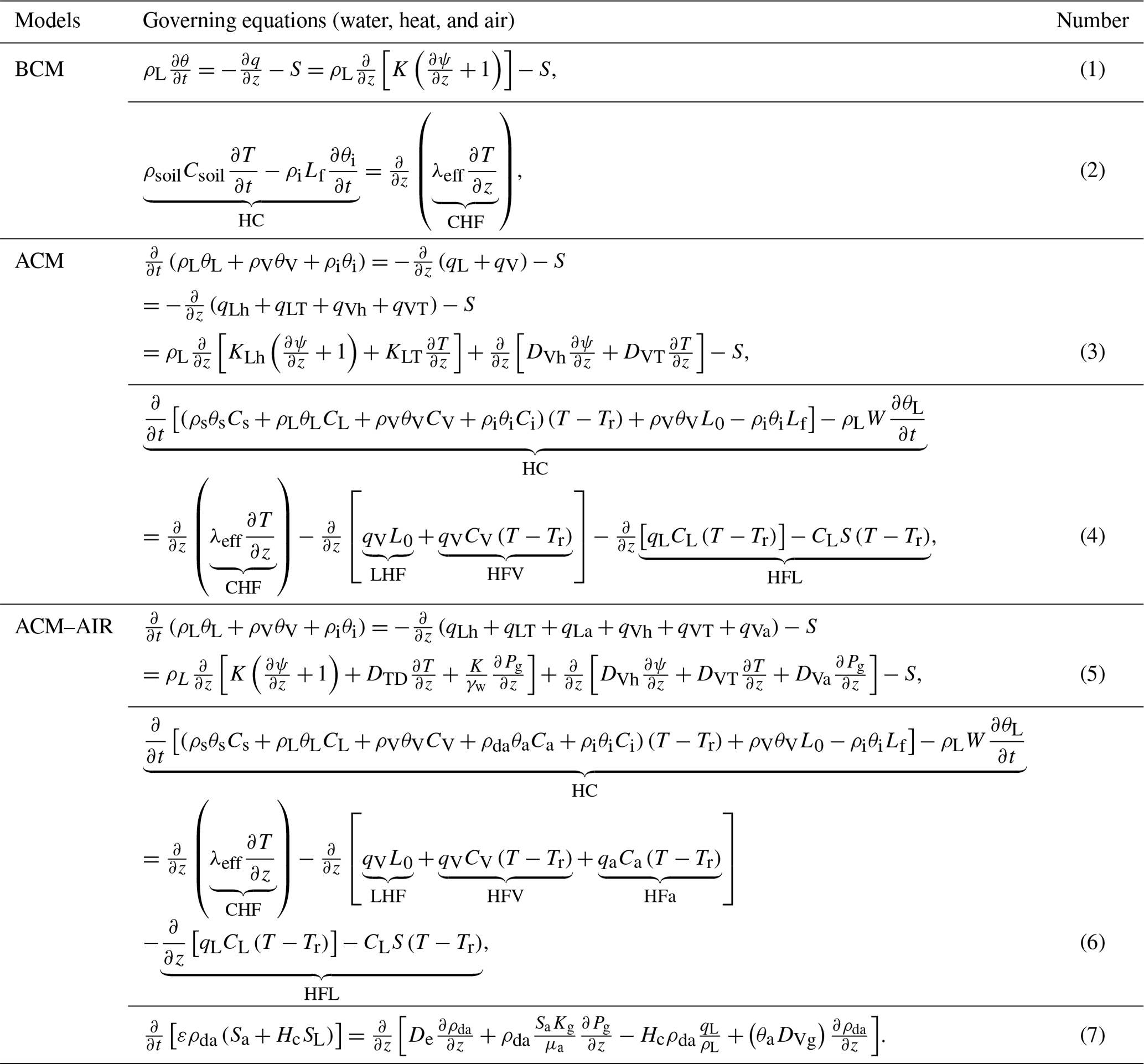
Table 1Governing equations for different complexities of water and heat coupling physics (see the Appendix for notations).
2.1 Experimental site
Maqu station, equipped with a catchment-scale soil moisture and soil temperature (SMST) monitoring network and micrometeorological observing system (Su et al., 2011; Dente et al., 2012; Zeng et al., 2016), is situated on the northeastern fringe of the Tibetan Plateau (33∘30′–34∘15′ N, 101∘38′–102∘45′ E). According to the updated Köppen–Geiger climate classification system, it can be characterized as a cold climate with a dry winter and warm summer (Dwb). The mean annual air temperature is 1.2 ∘C, and the mean air temperatures of the coldest month (January) and warmest month (July) are about −10.0 and 11.7 ∘C, respectively. Alpine meadows (e.g., Cyperaceae and Gramineae), with heights varying from 5 to 15 cm throughout the growing season, are the dominant land cover in this region. In situ soil sampling determined that the soil has a mixture of sandy loam, silt loam, and organic soil, with a maximum of 18.3 % organic matter for the upper soil layers (Dente et al., 2012; Zheng et al., 2015a; Zhao et al., 2018).
The Maqu SMST monitoring network spans an area of approximately 40 km × 80 km, with the elevation ranging from 3200 to 4200 m above sea level (a.s.l.). SMST profiles are automatically measured by 5TM ECH2O probes (Meter Group, Inc., USA) installed at the soil depths of 5, 10, 20, 40, and 80 cm. The micrometeorological observing system includes a 20 m planetary boundary layer (PBL) tower providing the meteorological measurements at five heights above ground (i.e., wind speed and direction, air temperature, and relative humidity), and an eddy covariance (EC150; Campbell Scientific, Inc., USA) system installed for measuring the turbulent, sensible, latent heat fluxes, and carbon fluxes. The four-component down and upwelling solar and thermal radiation (NR01-L; Campbell Scientific, Inc., USA) and liquid precipitation (T200B; Geonor, Inc., USA) are also monitored.
2.2 Mass and energy transport in unsaturated soils
On the basis of the STEMMUS modeling framework, the increasing complexity of vadose zone physics in frozen soils was implemented as three alternative models (Table 1). First, STEMMUS enabled isothermal water and heat transfer physics (Eqs. 1 and 2). The 1D Richards equation was utilized to solve the isothermal water transport in variably saturated soils. The heat conservation equation took into account the freezing and thawing process and the latent heat due to the water phase change. The effect of soil ice on soil hydraulic and thermal properties was considered. This is termed the basic coupled water and heat transfer model (BCM).
Second, the fully coupled water and heat physics, i.e., water vapor flow and thermal effect on water flow, was explicitly considered in STEMMUS and termed the advanced coupled model (ACM). For the ACM physics, the extended version of the Richards (1931) equation, with modifications made by Milly (1982), was used as the water conservation equation (Eq. 3). Water flow can be expressed as liquid and vapor fluxes driven by both temperature gradients and matric potential gradients. The heat transport in frozen soils mainly includes heat conduction (CHF; ), convective heat transferred by liquid flux (HFL; , ), vapor flux (HFV; ), the latent heat of vaporization (LHF; −qVL0), the latent heat of freezing or thawing (−ρiθiLf), and a source term associated with the exothermic process of the wetting of a porous medium (integral heat of wetting) (). It can be expressed as Eq. (4) (De Vries, 1958; Hansson et al., 2004).
Lastly, STEMMUS expressed the freezing soil porous medium as the mutually dependent system of liquid water, water vapor, ice water, dry air, and soil grains in which, other than airflow, all other components are kept the same as in ACM (termed the ACM–AIR model; Eqs. 5–7; Zeng et al., 2011a, b; Zeng and Su, 2013). The effect of airflow on soil water and heat transfer can be two-fold. First, the airflow-induced water and vapor fluxes (qLa, qVa) and the corresponding convective heat flow (HFa; ) were considered. Second, the presence of airflow alters the vapor transfer processes, which can considerably affect the water and heat transfer in an indirect manner.
STEMMUS utilized the adaptive time step strategy, with maximum time steps ranging from 1 to 1800 s (e.g., with 1800 s as the time step under stable conditions). The maximum desirable change in soil moisture and soil temperature within one time step was set as 0.02 cm3 cm−3 and 2 ∘C, respectively, to prevent too large a change in state variables that may cause numerical instabilities. If the changes between two adjacent soil moisture and temperature states are less than the maximum desirable change, STEMMUS continues without changing the length of current time step (e.g., 1800 s). Otherwise, STEMMUS will adjust the time step with a deduction factor, which is proportional to the difference between the changes that are too large and the maximum that are desirable in state variables. Within one single time step, the Picard iteration was used to solve the numerical problem, and the numerical convergence criteria is set as 0.001 for both soil matric potential (in centimeters) and soil temperature (in degrees Celsius).
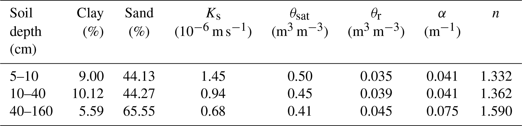
To accommodate the specific conditions of a Tibetan meadow, the total depth of the soil column was set as 1.6 m (Fig. 1). The vertical soil discretization was designed to be finer for the upper soil layers (0.1–2.5 cm for 0–40 cm; 27 layers) than for the lower soil layers (5–20 cm for 40–160 cm; 10 layers). The surface boundary for the water transport was set as the flux-type boundary controlled by the atmospheric forcing (i.e., evaporation and precipitation), while the specific soil temperature was assigned as the surface boundary of the energy conservation equation. The free drainage (zero matric potential gradient) and measured soil temperature were set as the bottom boundary conditions for the water transport and heat transport, respectively. For the airflow, the surface boundary was set as the atmospheric pressure, and soil air was allowed to escape from the bottom of the soil column. Surface evapotranspiration was calculated using the Penman–Monteith method. Soil evaporation and transpiration can be separately estimated. The available radiation energy is partitioned into the canopy and soil component via the leaf area index (LAI); the canopy minimum surface resistance and soil surface resistance are then utilized to calculate the potential transpiration and soil evaporation. Actual transpiration is calculated as the function of potential transpiration and the root-length-density-weighted available soil liquid water (which is assumed to be zero if soil temperature falls below 0 ∘C; Kroes et al., 2009; Orgogozo et al., 2019). For our simulation period, grassland stepped into the dormancy period as the soil froze. The accumulative positive temperature during the thawing period was not enough to break the dormancy of the vegetation. The contribution of plant transpiration to the land surface heat flux is negligible during the dormancy period. The effect of soil moisture on the actual soil evaporation is taken into account via the soil surface resistance (Eq. A6). All three aforementioned models adopted the same adaptive time step strategy and numerical solution and the same soil discretization, soil parameters (shown in Table 2), and boundary conditions. It indicated that the truncation errors, due to the numerical solution, among the three models were comparable. The differences among the models were mainly restricted to the various representations of soil physical processes (e.g., the inclusion of vapor flow and airflow or not).
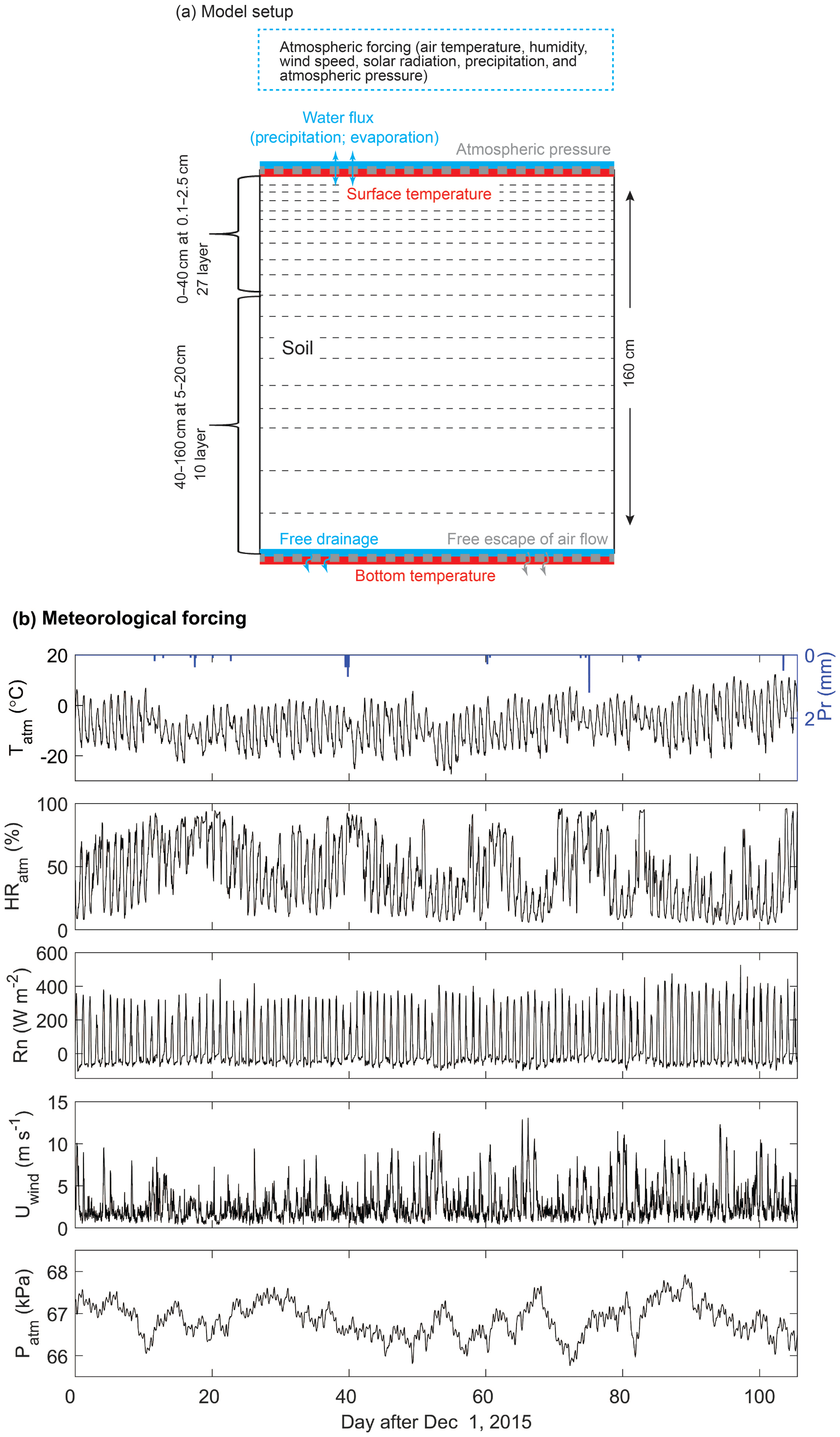
Figure 1(a) Conceptual illustration of the model setup, the surface and bottom boundary conditions, driving forces, and vertical discretization. (b) Half-hourly measurements of meteorological forcing, including air temperature (Tatm, ∘C), relative humidity (HRatm, %), net radiation (Rn, W m−2), wind speed (Uwind, m s−1), and atmospheric pressure (Patm, kPa) during the simulation period. Note that the dimensions are not drawn to scale; models were run at a 1D scale.
Table 2The adopted average values of soil texture and hydraulic properties at different depths (see the Appendix for the notations).
Given the same atmospheric forcing and the same set of parameters, the performance of models with varying complexities of soil water and heat physics was illustrated in Sect. 3.1–3.3. Section 3.4 and 3.5 further analyzed the variations in heat budgets and subsurface latent heat flux density, illustrating differences in the underlying mechanisms among various models.
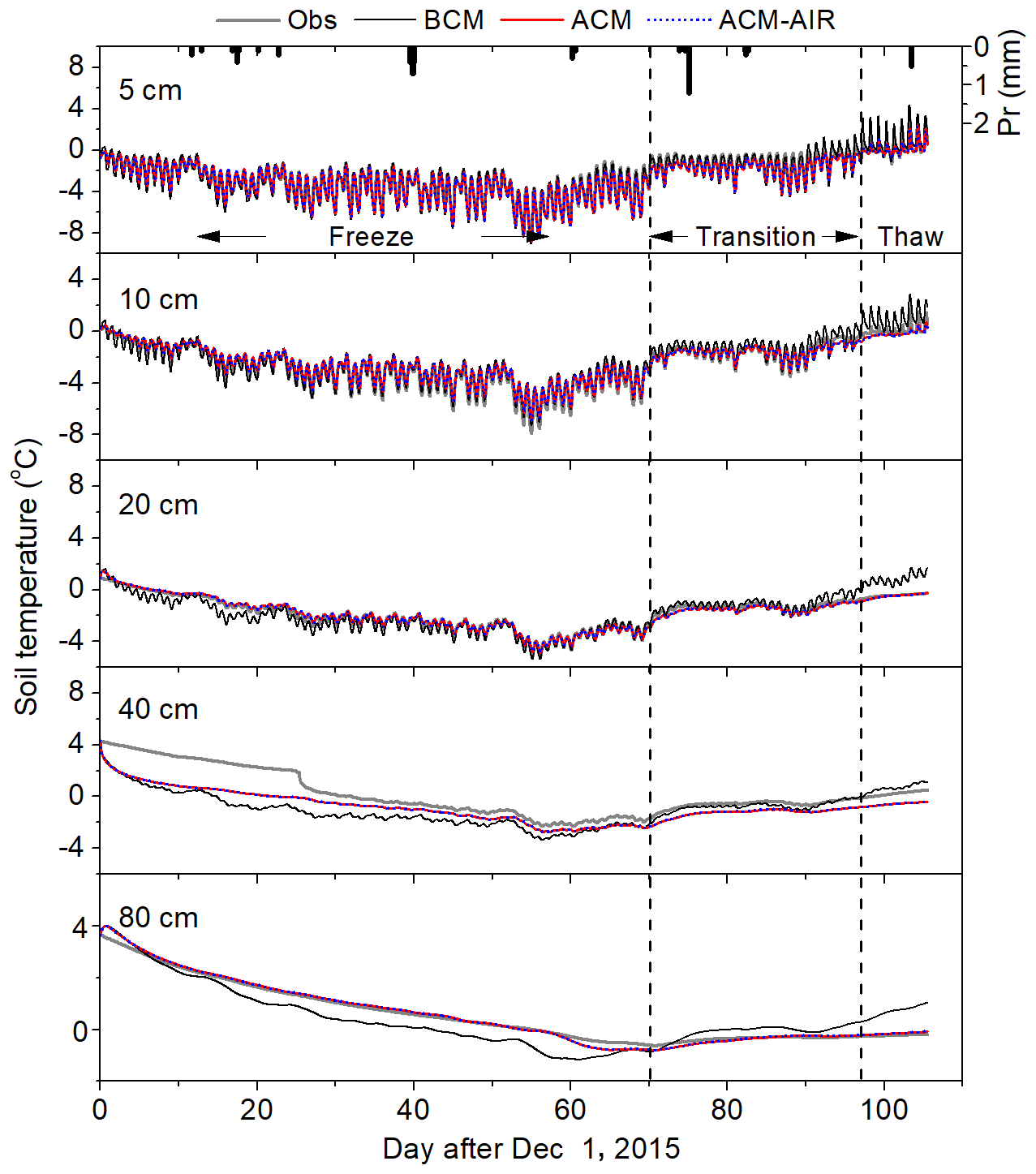
Figure 2Comparison of measured (Obs) and estimated time series of soil temperature at various soil layers using the basic coupled model (BCM), advanced coupled model (ACM), and advanced coupled model with airflow (ACM–AIR).
3.1 Soil hydrothermal profile simulations
The performance of the model, with various soil physics, simulating the soil thermal profile information is illustrated in Fig. 2. Both ACM and ACM–AIR reproduced the time series of the soil temperature at different soil depths well, except at 40 cm which is most probably due to inappropriate measurements (e.g., improper placement of sensors). However, there are significant discrepancies in soil temperature simulated by the BCM. Compared to the observations, a stronger diurnal behavior of soil temperature, in response to the fluctuating atmospheric forcing, was found, and an earlier stepping in and stepping out of the frozen period was simulated by the BCM. Such differences enlarged at deeper soil layers, with large bias and root mean square error (RMSE) values (Table 3).
Table 3Comparative statistical values of observed and simulated soil temperature and moisture with three models, with the bold font indicating the best statistical performance.
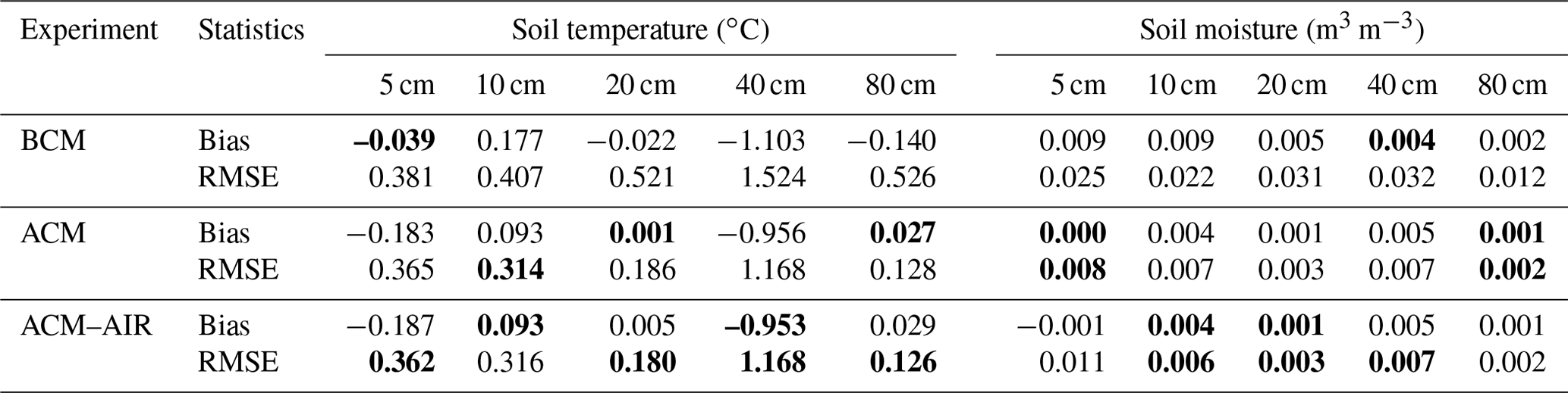
Note: , , where yi, are the measured and model-simulated soil temperature or moisture, and n is the number of data points.

Figure 3Comparison of measured (Obs) and model-simulated time series of soil moisture at various soil layers using the basic coupled model (BCM), advanced coupled model (ACM), and advanced coupled model with airflow (ACM–AIR).
Figure 3 presents the time series of observed and simulated soil liquid water content at five soil layers. During the rapid freezing period, a noticeable overestimation of the diurnal fluctuations and an early and fast decrease in soil liquid water content was simulated by BCM. Moreover, stronger diurnal fluctuations and an early increase in liquid water content were also found during the thawing period. The early thawing of soil water even led to an unrealistic refreezing process at 80 cm (from the 88th to 92nd day after December 2015), which is due to the simulated early warming of soil by BCM (Fig. 2). Such discrepancies were significantly ameliorated by ACM and ACM–AIR simulations. Nevertheless, all three models can capture the diurnal variations in and magnitude of liquid water content during the frozen period well. Note that there is an observable difference between ACM- and ACM–AIR-simulated soil liquid water content at shallower soil layers during the thawing process (e.g., Fig. 3; 5 cm).
3.2 Freezing front propagation
The time series of freezing front propagation derived from the measured and simulated soil temperature was reproduced in Fig. 4. Initialized from the soil surface, the freezing front quickly develops downwards until the maximum freezing depth is reached. The thawing process starts from both the top and bottom and is mainly driven by the atmospheric heat and bottom soil temperature, respectively. Such characteristics were captured well by both the ACM and ACM–AIR models in terms of freezing rate, maximum freezing depth, and surface thawing process, while the BCM tended to present a more fluctuating and rapidly freezing front propagation and a deeper maximum freezing depth that was reached early. The effect of atmospheric heat sources on the soil was overestimated by the BCM, as shown by the stronger diurnal early onset of the thawing process.
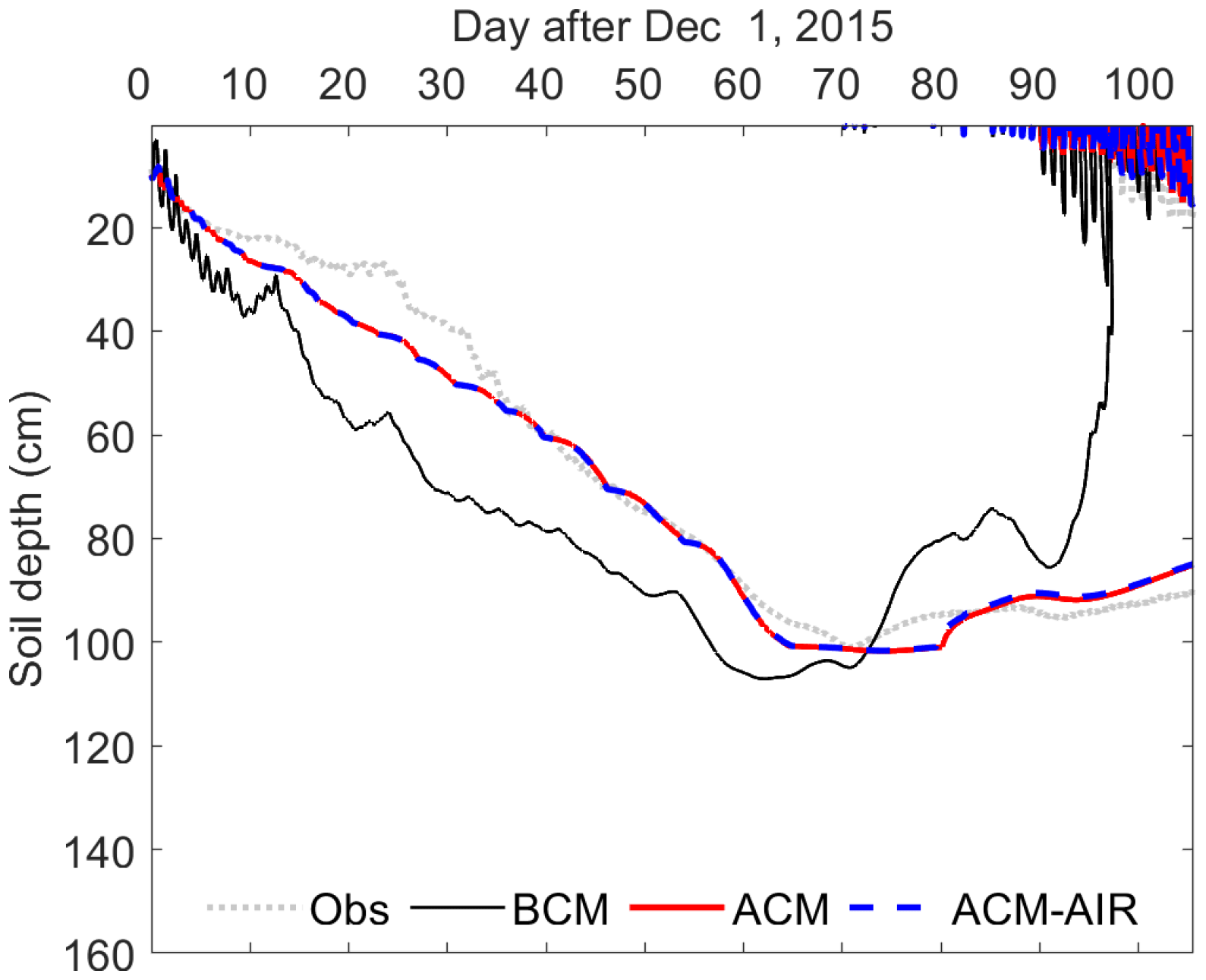
Figure 4Comparison of measured (Obs) and model-simulated freezing front propagation (FFP) using the basic coupled model (BCM), advanced coupled model (ACM), and advanced coupled model with airflow (ACM–AIR). Note that the measured FFP was seen as the development of zero degree isothermal lines from the measured soil temperature field.
3.3 Surface evapotranspiration
The performance of the model with different soil physics in reproducing the latent heat flux dynamics is shown in Fig. 5. Compared to the observed LE, there is a significant overestimation of the half-hourly latent heat flux, which significantly degraded the overall performance when using BCM. The occurrence of such an overestimation was notably reduced when using ACM and ACM–AIR. The general underestimation of the latent heat flux by the ACM and ACM–AIR was found mostly during the freezing–thawing transition period (Fig. 6b) when the soil hydrothermal states are not well captured (Figs. 2 and 3).
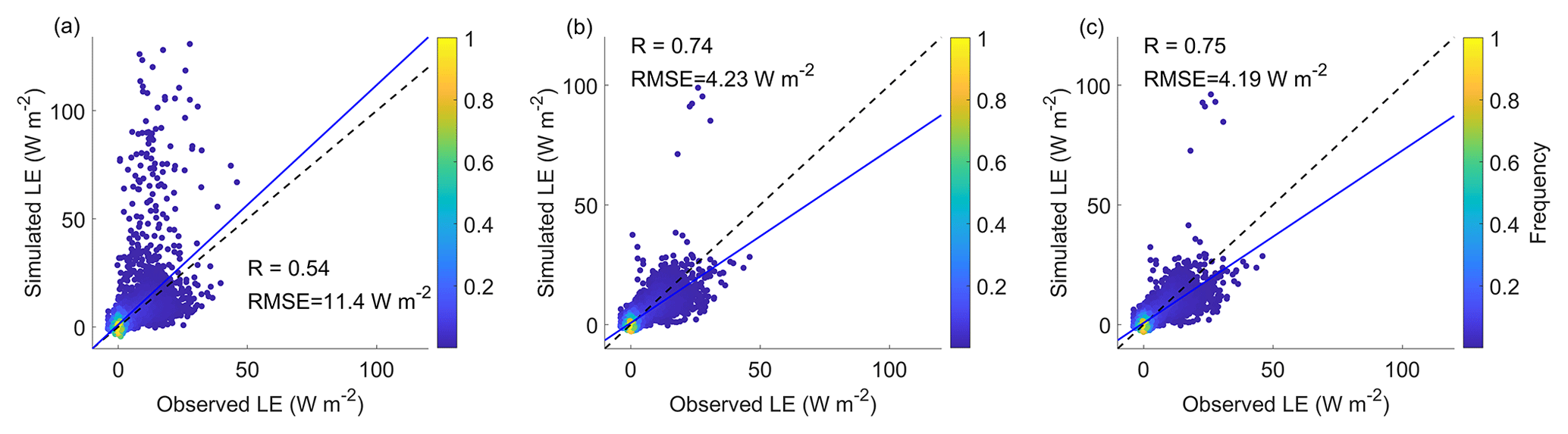
Figure 5Scatterplot of observed and model-estimated half-hourly latent heat flux using the (a) basic coupled model (BCM), (b) advanced coupled model (ACM), and (c) advanced coupled model with airflow (ACM–AIR). The color indicates the data composite of surface latent heat flux.
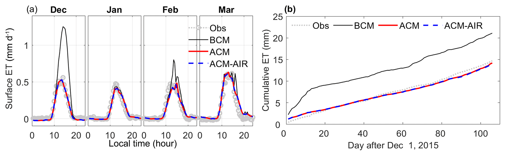
Figure 6Comparison of observed and model-simulated (a) mean diurnal variations in surface evapotranspiration and (b) cumulative evapotranspiration (ET) by the basic coupled model (BCM), advanced coupled model (ACM), and advanced coupled model with airflow (ACM–AIR).
The overestimation of surface evapotranspiration by BCM was significant during the initial freezing and transition period (Fig. 6a; December and February). During the rapid freezing period (January), BCM presented a good match in the diurnal variation as compared to the observations. The monthly average diurnal variations were found to be well captured by ACM and ACM–AIR. Figure 6b shows the comparison of observed and simulated cumulative surface evapotranspiration. The overall overestimation of surface evapotranspiration by BCM can be clearly seen in Fig. 6b. Days in the initial freezing periods, with high liquid water content simulations, accounted for more than 90 % of the overestimation. The initial stage overestimation of surface evapotranspiration was significantly reduced by ACM and ACM–AIR. A slight underestimation of cumulative surface evapotranspiration was simulated by ACM and ACM–AIR, with values of 3.98 % and 4.78 %, respectively.
3.4 Heat budgets
Figure 7 shows the time series of simulated energy budget components at 5 cm using BCM, ACM, and ACM–AIR during the freezing period (5th–11th day after 1 December) and the freezing–thawing transition period (83rd–89th day after 1 December). For the BCM, only the change rate of heat content (HC) and conductive heat flux divergence (CHF) are considered in the left-hand side (LHS) and right-hand side (RHS) of Eq. (2); see Table 1. Three additional terms, namely convective heat flux divergence of liquid flow (HFL) and vapor flow (HFV) and latent heat flux divergence, were included for the ACM, while for the ACM–AIR the convective heat flux divergence of airflow (HFa) was also added.
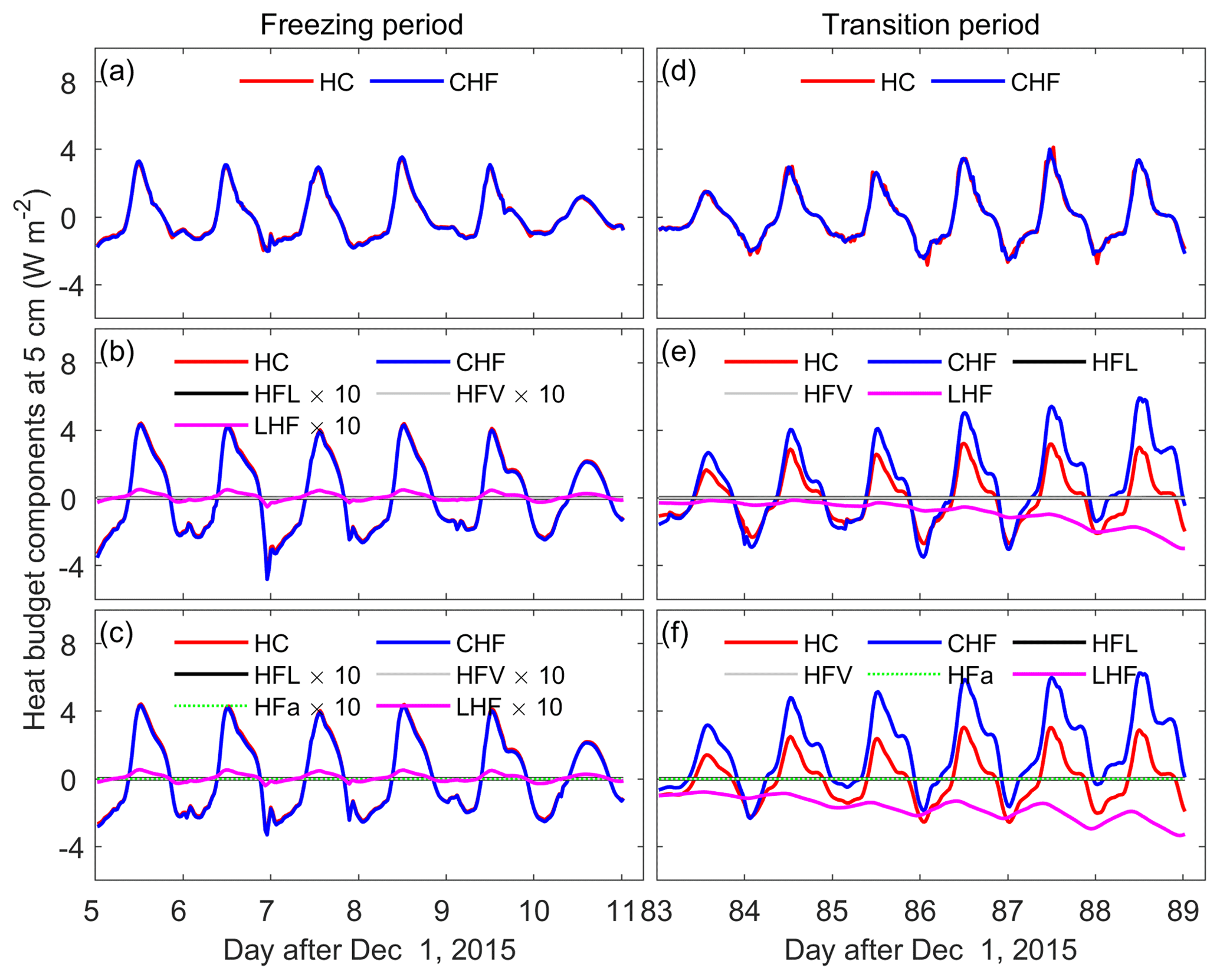
Figure 7Time series of model-simulated heat budget components at the soil depth of 5 cm, using the (a, d) basic coupled model (BCM), (b, e) advanced coupled model (ACM), and (c, f) advanced coupled model with airflow (ACM–AIR) simulations during the typical 6 d freezing (a–c) and freezing–thawing transition (d–f) periods. HC – change rate of heat content; CHF – conductive heat flux divergence; HFL – convective heat flux divergence due to liquid water flow; HFV – convective heat flux divergence due to water vapor flow; HFa – convective heat flux divergence due to airflow; and LHF – latent heat flux divergence. Note that, for graphical purposes, HFL, HFV, HFa, and LHF were enhanced by a factor of 10 during the freezing period.
There is a strong diurnal variation in heat budget components (HC, CHF, and LHF; Table 1) corresponding to the diurnal fluctuation in soil temperature. For the BCM, the change rate of the heat content was almost completely balanced by the conductive heat flux divergence (CHF; Fig. 7a). Compared to the BCM, a stronger diurnal fluctuation of HC and CHF was found in ACM results. As inferred from the results in Fig. 2, the time series of soil temperature change () simulated by BCM was larger than that simulated by ACM. This indicates that BCM produced less fluctuation in apparent heat capacity () than ACM. During the freezing period, the latent heat flux divergence (LHF) was lower than the conductive heat flux divergence (CHF) by 1–2 orders of magnitude (Fig. 7b). The positive value of the LHF term during the daytime indicates that condensation happens at 5 cm as the water vapor moves downward. The convective heat fluxes of liquid flow and vapor flow were even smaller compared to conductive heat flux (Fig. 7b). There is no significant difference in heat budget components between ACM and ACM–AIR in terms of diurnal variation and magnitude. The convective heat flux divergence of airflow played a negligible role in the change in the thermal state (HC) (Fig. 7c).
The dynamics of heat balance components at the 5 cm soil layer were simulated for the freezing–thawing transition period (Fig. 7d–f). Both HC and CHF underwent strong diurnal variations with increasing fluctuation magnitude, indicating soil warming at 5 cm. For the ACM, CHF outnumbered HC during daytime, and the difference increased with time. Negative values were found for LHF and developed further over time. The sum of CHF and LHF nearly balanced the HC term. Such behavior was similarly reproduced by ACM–AIR, with a slightly larger difference between the HC and CHF terms. This means a larger amount of water vapor was evaporated from the 5 cm soil layer (with a more negative LHF term) from ACM–AIR simulations than that from ACM simulations, which explains the lower liquid water content for ACM–AIR (Fig. 3; 5 cm).
3.5 Subsurface latent heat flux density
To give more context to the results, the spatial and temporal distributions of the simulated latent heat flux density (Sh), namely , during the freezing and freezing–thawing transition period are shown in Fig. 8. For the BCM, the latent heat flux density (Sh) is not available as it neglects the vapor flow.

Figure 8The spatial and temporal distributions of model-estimated soil latent heat flux density using the (a, d) advanced coupled model (ACM), (b, e) advanced coupled model with airflow (ACM–AIR), and (c, f) the difference between ACM and ACM–AIR simulations () during the typical 6 d freezing and freezing–thawing transition periods. The left (a–c) and right (d–f) columns are for the freezing and freezing–thawing transition periods, respectively. Note that figures for the basic coupled model (BCM) are absent as the model cannot simulate the subsurface soil latent heat flux density.
Figure 8a shows that there is a strong diurnal variation of Sh in the upper 0.1 cm soil layers. Such diurnal behavior along the soil profile was interrupted at 1 cm, at which point the water vapor consistently moved upwards as an evaporation source (termed as evaporative front). The path of this upward water vapor was disrupted at 20 cm from 6 December onward when the freezing front developed. Compared to the upper 0.1 cm soil, a weaker diurnal fluctuation of Sh was found at lower soil layers. For ACM–AIR, the vapor transfer patterns were similar to those of ACM (Fig. 8b). There were isolated connections of condensed water vapor between the upper 1 cm of soil and the lower soil layers (Sh>0; e.g., 6, 7, 9, and 10 December), possibly associated with the downward airflow (see Fig. 12 in Yu et al., 2018). The large difference in magnitude of latent heat flux density between ACM and ACM–AIR appeared to be mainly isolated in the upper soil layers (Fig. 8c). At soil layers between 1 and 20 cm, ACM–AIR simulated less in the condensation vapor area (Sh>0) and more in the evaporation area (Sh<0), indicating that ACM–AIR produced an additional amount of condensation and evaporation water vapor compared with ACM (Fig. 8c).
Similar to during the freezing period, the Sh during the transition period can be characterized as having strong diurnal variations at upper soil layers, interrupting diurnal patterns with the constant upward evaporation of intermediate soil layers, and having weak diurnal variations at lower soil layers (Fig. 8d and e). While the maximum evaporation rate was less than that during the freezing period, the consistent evaporation zone developed to a depth of 5 cm. The path for the upward-moving water vapor tended to develop deeper than 30 cm with the absence of soil ice. The simulation by ACM–AIR produced more condensation and less evaporative water vapor than that of ACM (Fig. 8f). In addition, steadily more evaporative water vapor from 5 cm was simulated by ACM–AIR compared to ACM. This confirms the aforementioned point that, during the freezing–thawing transition period, large LHF values were simulated by ACM–AIR (Fig. 7).
4.1 Coupled water and heat transfer processes
Vapor flow, which is dependent on soil matric potential and temperature, links soil water and heat transfer processes. The mutual dependence of soil water in different phases (liquid, water vapor, and ice) and heat transport on vapor flow enables the facilitation of our better understanding of the complex soil physical processes (e.g., Figs. 7–8). Specifically, the interdependence of soil moisture and soil temperature (SMST) profiles simulated by ACM was closer to the observation than that by BCM. In addition, a significant enhancement in the portrayal of the monthly average diurnal variations in surface evapotranspiration and cumulative evapotranspiration can be found in ACM simulations which constrain the hydrothermal regimes, especially during the freezing–thawing transition periods (Figs. 2, 3, and 6).
During the freezing period, liquid water in the soil freezes, which is analogous to the soil drying process, and water vapor fluxes instead of liquid fluxes dominate the mass transfer process (Zhang et al., 2016). Neglecting such an important water flux component unavoidably results in different or unrealistic simulations of surface evapotranspiration and SMST profiles (Li et al., 2010; Karra et al., 2014; Wang and Yang, 2018). Li et al. (2010) reported that vapor fluxes were comparable to the liquid water fluxes and affected the freezing and melting processes. On the basis of long-term 1D soil column simulations, Karra et al. (2014) reported that the inclusion of the vapor diffusion effect significantly increased the thickness of the ice layer, as explained by the positive vapor cold trapping–thermal conductivity feedback mechanism. From the energy budget perspective, latent heat fluxes contribute more, due to the vapor phase change (LHF), to the heat balance budget at soil layers above the evaporative front than that below it (see LHF in Fig. 7e vs. Fig. 7b; corresponding evaporative front shown in Fig. 8d vs. Fig. 8a). This is consistent with findings by Zhang et al. (2016), who concluded that the latent heat of vapor, due to phase change, is 2 orders of magnitude less than the heat fluxes, due to conduction during wintertime. This corresponds to our results in Fig. 7b and c during the freezing period, while our results further showed that the latent heat fluxes, due to vapor phase change, can be considerable during the transition period (Fig. 7e and f). The downward latent heat flux from ACM makes the subsurface soil warmer, which reduces the temperature gradient () (Wang and Yang, 2018). This further results in weaker diurnal fluctuations of the HC term in ACM than in BCM (see HC in Fig. 7e vs. Fig. 7d). At the soil layers below the evaporative front, the heat flux source from the vapor transfer process (LHF) is negligible (e.g., Fig. 7b). The thermal retard effect occurs as the presence of soil ice, expressed as the apparent heat capacity term (Capp), dominates the heat transfer process in frozen soils. By considering the thermal effect on water flow, ACM usually has a larger water capacity value than BCM does. As such, the intense thermal impedance effect leads to the result that ACM produced a weaker diurnal fluctuation of soil temperature than BCM at subsurface soil layers (e.g., Fig. 2; 20 cm).
4.2 Airflow in the soil
Since soil pores are filled with liquid water, vapor, and dry air, taking dry air as an independent state variable can facilitate a better understanding of the relative contribution of each component to the mass and heat transfer in soils. The results show that the dry-air-induced water and heat flow is negligible in relation to the total mass and energy transfer (Zeng et al., 2011b; Yu et al., 2018). Nevertheless, dry air can affect soil hydrothermal regimes significantly under certain circumstances. Wicky and Hauck (2017) reported that the airflow-induced convective heat transfer resulted in a considerable temperature difference between the upper and lower part of a permafrost talus slope and, thus, had a remarkable effect on the thermal regime of the talus slope. Zeng et al. (2011b) demonstrated that the airflow-induced surface evaporation enhanced after precipitation events, since the hydraulic conductivity of topsoil layers increased tremendously due to the increased topsoil moisture by the injected airflow from the moist atmosphere. In this study, we found that the explicit consideration of airflow introduced an additional amount of subsurface condensation and evaporative water vapor in the condensation region and evaporation region, respectively (Fig. 8c and f). The effect of latent heat flux on heat transfer was enhanced by airflow during the freezing–thawing transition period (Fig. 7), which further affected the subsurface hydrothermal simulations (e.g., Fig. 3).
On the basis of the STEMMUS modeling framework, with various representations of water and heat transfer physics (BCM, ACM, and ACM–AIR), the performance of each model in simulating water and heat transfer and surface evapotranspiration was evaluated over a typical Tibetan meadow ecosystem. Results indicated that, compared to in situ observations, the BCM tended to present earlier freezing and thawing dates, with a stronger diurnal variation in soil temperature and liquid water in response to the atmospheric forcing. Such discrepancies were considerably reduced by the model with the advanced coupled water–heat physics. Surface evapotranspiration was overestimated by BCM, mainly due to the mismatches during the initial freezing and freezing–thawing transition period. ACM models, with the coupled constraints from the perspective of water and energy conservation, significantly improve the model performance in mimicking the surface evapotranspiration dynamics during the frozen period. The analysis of the heat budget components and latent heat flux density revealed that the improvement in soil temperature simulations by ACM is ascribed to its physical consideration of vapor flow and the thermal effect on water flow, with the former mainly functioning at regions above the evaporative front and the latter dominating below the evaporative front. The nonconductive heat process (liquid or vapor or air-induced heat convection flux) contributed very minimally to the total energy fluxes during the frozen period, except for the latent heat flux divergence at the topsoil layers. The contribution of airflow-induced water and heat flow to the total mass and energy fluxes is negligible. However, given the explicit consideration of airflow, the latent heat flux and its effect on heat transfer were enhanced during the freezing–thawing transition period. This work highlighted the role of considering the vapor flow and the thermal effect on water flow and airflow in portraying the subsurface soil hydrothermal dynamics, especially during freezing–thawing transition periods. To sum up, this study can contribute to a better understanding of the freeze–thaw mechanisms of frozen soils, which will subsequently contribute to the quantification of permafrost carbon feedback (Burke et al., 2013; Kevin et al., 2014; Schuur et al., 2015) if the STEMMUS–FT model is coupled with a biogeochemical model, as has been implemented lately (Yu et al., 2020a).
The one-step calculation of actual soil evaporation (Es) and potential transpiration (Tp) is achieved by incorporating canopy minimum surface resistance and actual soil resistance into the Penman–Monteith model (i.e., the ETdir method in Yu et al., 2016). LAI is implicitly used to partition available radiation energy into the radiation reaching the canopy and soil surface.
where and (MJ m−2 d−1) are the net radiation at the canopy surface and soil surface, respectively; ρa (kg m−3) is the air density; cp (J kg−1 K−1) is the specific heat capacity of air; and (s m−1) are the aerodynamic resistance for canopy surface and soil surface, respectively; rc,min (s m−1) is the minimum canopy surface resistance; and rs (s m−1) is the soil surface resistance.
The net radiation reaching the soil surface can be calculated using Beer's law as follows:
And the net radiation intercepted by the canopy surface is the residual part of total net radiation, as follows:
The minimum canopy surface resistance rc,min is given by the following:
where rl,min is the minimum leaf stomatal resistance and LAIeff is the effective leaf area index, which considers that, generally, the upper and sunlit leaves in the canopy actively contribute to the heat and vapor transfer.
The soil surface resistance can be estimated following van de Griend and Owe (1994):
where rsl (10 s m−1) is the resistance to molecular diffusion of the water surface, a (0.3565) is the fitted parameter, θ1 is the topsoil water content, and θmin is the minimum water content above which soil is able to deliver vapor at a potential rate.
The root water uptake term described by Feddes et al. (1978) is as follows:
where α(h) (dimensionless) is the reduction coefficient related to soil water potential h, and Sp (s−1) is the potential water uptake rate.
where b(z) is the normalized water uptake distribution, which describes the vertical variation of the potential extraction term, Sp, over the root zone. Here the asymptotic function was used to characterize the root distribution as described in Gale and Grigal (1987), Jackson et al. (1996), Yang et al. (2009), and Zheng et al. (2015b). Tp is the potential transpiration in Eq. (A1).
The soil hydraulic and thermal property data can be freely downloaded from the 4TU. Center for Research Data (https://doi.org/10.4121/uuid:61db65b1-b2aa-4ada-b41e-61ef70e57e4a; Zhao et al., 2020). Some relevant data are made available from the 4TU. Center for Research Data (https://doi.org/10.4121/uuid:cc69b7f2-2448-4379-b638-09327012ce9b; Yu et al., 2020b).
ZS and YZ conceptualized the study, while LY and YZ developed the methodology and prepared the original draft of the paper. LY, YZ, and ZS all contributed to the reviewing and editing of the final paper.
The authors declare that they have no conflict of interest.
This article is part of the special issue “Data acquisition and modeling of hydrological, hydrogeological and ecohydrological processes in arid and semi-arid regions”. It is not associated with a conference.
The authors thank the editor and referees very much for their constructive comments, which improved the paper.
This research has been supported by the National Natural Science Foundation of China (grant no. 41971033) and the Fundamental Research Funds for the Central Universities (CHD; grant no. 300102298307).
This paper was edited by Philip Brunner and reviewed by Orgogozo Laurent and one anonymous referee.
Bao, H., Koike, T., Yang, K., Wang, L., Shrestha, M., and Lawford, P.: Development of an enthalpy-based frozen soil model and its validation in a cold region in China, J. Geophys. Res.-Atmos., 121, 5259–5280, https://doi.org/10.1002/2015jd024451, 2016.
Biskaborn, B. K., Smith, S. L., Noetzli, J., Matthes, H., Vieira, G., Streletskiy, D. A., Schoeneich, P., Romanovsky, V. E., Lewkowicz, A. G., Abramov, A., Allard, M., Boike, J., Cable, W. L., Christiansen, H. H., Delaloye, R., Diekmann, B., Drozdov, D., Etzelmüller, B., Grosse, G., Guglielmin, M., Ingeman-Nielsen, T., Isaksen, K., Ishikawa, M., Johansson, M., Johannsson, H., Joo, A., Kaverin, D., Kholodov, A., Konstantinov, P., Kröger, T., Lambiel, C., Lanckman, J.-P., Luo, D., Malkova, G., Meiklejohn, I., Moskalenko, N., Oliva, M., Phillips, M., Ramos, M., Sannel, A. B. K., Sergeev, D., Seybold, C., Skryabin, P., Vasiliev, A., Wu, Q., Yoshikawa, K., Zheleznyak, M., and Lantuit, H.: Permafrost is warming at a global scale, Nat. Commun., 10, 264, https://doi.org/10.1038/s41467-018-08240-4, 2019.
Boone, A., Masson, V., Meyers, T., and Noilhan, J.: The Influence of the Inclusion of Soil Freezing on Simulations by a Soil–Vegetation–Atmosphere Transfer Scheme, J. Appl. Meteorol., 39, 1544–1569, https://doi.org/10.1175/1520-0450(2000)039<1544:TIOTIO>2.0.CO;2, 2000.
Burke, E. J., Jones, C. D., and Koven, C. D.: Estimating the Permafrost-Carbon Climate Response in the CMIP5 Climate Models Using a Simplified Approach, J. Climate, 26, 4897–4909, https://doi.org/10.1175/jcli-d-12-00550.1, 2013.
Cheng, G. and Wu, T.: Responses of permafrost to climate change and their environmental significance, Qinghai-Tibet Plateau, J. Geophys. Res.-Earth, 112, F02S03, https://doi.org/10.1029/2006JF000631, 2007.
Cuntz, M. and Haverd, V.: Physically Accurate Soil Freeze-Thaw Processes in a Global Land Surface Scheme, J. Adv. Model. Earth Syst., 10, 54–77, https://doi.org/10.1002/2017MS001100, 2018.
Dente, L., Vekerdy, Z., Wen, J., and Su, Z.: Maqu network for validation of satellite-derived soil moisture products, Int. J. Appl. Earth Obs. Geoinf., 17, 55–65, https://doi.org/10.1016/j.jag.2011.11.004, 2012.
De Vries, D. A.: Simultaneous transfer of heat and moisture in porous media, Eos Trans. AGU, 39, 909–916, https://doi.org/10.1029/TR039i005p00909, 1958.
De Vries, D. A.: The theory of heat and moisture transfer in porous media revisited, Int. J. Heat Mass Tran., 30, 1343–1350, https://doi.org/10.1016/0017-9310(87)90166-9, 1987.
Feddes, R. A., Kowalik, P. J., and Zaradny, H.: Simulation of field water use and crop yield, Centre for Agricultural Publishing and Documentation, Wageningen, the Netherlands, 189 pp., 1978.
Flerchinger, G. N. and Saxton, K. E.: Simultaneous heat and water model of a freezing snow-residue-soil system. I. Theory and development, T. ASABE, 32, 565–571, https://doi.org/10.13031/2013.31040, 1989.
Gale, M. R. and Grigal, D. F.: Vertical root distributions of northern tree species in relation to successional status, Can. J. Forest Res., 17, 829–834, https://doi.org/10.1139/x87-131, 1987.
Grenier, C., Anbergen, H., Bense, V., Chanzy, Q., Coon, E., Collier, N., Costard, F., Ferry, M., Frampton, A., Frederick, J., Gonçalvès, J., Holmén, J., Jost, A., Kokh, S., Kurylyk, B., McKenzie, J., Molson, J., Mouche, E., Orgogozo, L., Pannetier, R., Rivière, A., Roux, N., Rühaak, W., Scheidegger, J., Selroos, J. O., Therrien, R., Vidstrand, P., and Voss, C.: Groundwater flow and heat transport for systems undergoing freeze-thaw: Intercomparison of numerical simulators for 2D test cases, Adv. Water Resour., 114, 196–218, https://doi.org/10.1016/j.advwatres.2018.02.001, 2018.
Guymon, G. L. and Luthin, J. N.: A coupled heat and moisture transport model for Arctic soils, Water Resour. Res., 10, 995–1001, https://doi.org/10.1029/WR010i005p00995, 1974.
Hansson, K., Šimůnek, J., Mizoguchi, M., Lundin, L. C., and van Genuchten, M. T.: Water flow and heat transport in frozen soil: Numerical solution and freeze-thaw applications, Vadose Zone J., 3, 693–704, https://doi.org/10.2136/vzj2004.0693, 2004.
Harlan, R. L.: Analysis of coupled heat-fluid transport in partially frozen soil, Water Resour. Res., 9, 1314–1323, https://doi.org/10.1029/WR009i005p01314, 1973.
Hinzman, L. D., Deal, C. J., McGuire, A. D., Mernild, S. H., Polyakov, I. V., and Walsh, J. E.: Trajectory of the Arctic as an integrated system, Ecol. Appl., 23, 1837–1868, https://doi.org/10.1890/11-1498.1, 2013.
Iijima, Y., Ohta, T., Kotani, A., Fedorov, A. N., Kodama, Y., and Maximov, T. C.: Sap flow changes in relation to permafrost degradation under increasing precipitation in an eastern Siberian larch forest, Ecohydrology, 7, 177–187, https://doi.org/10.1002/eco.1366, 2014.
Jackson, R. B., Canadell, J., Ehleringer, J. R., Mooney, H. A., Sala, O. E., and Schulze, E. D.: A Global Analysis of Root Distributions for Terrestrial Biomes, Oecologia, 108, 389–411, https://doi.org/10.1007/BF00333714, 1996.
Karra, S., Painter, S. L., and Lichtner, P. C.: Three-phase numerical model for subsurface hydrology in permafrost-affected regions (PFLOTRAN-ICE v1.0), The Cryosphere, 8, 1935–1950, https://doi.org/10.5194/tc-8-1935-2014, 2014.
Kevin, S., Hugues, L., Vladimir, E. R., Edward, A. G. S., and Ronald, W.: The impact of the permafrost carbon feedback on global climate, Environ. Res. Lett., 9, 085003, https://doi.org/10.1088/1748-9326/9/8/085003, 2014.
Koren, V., Schaake, J., Mitchell, K., Duan, Q. Y., Chen, F., and Baker, J. M.: A parameterization of snowpack and frozen ground intended for NCEP weather and climate models, J. Geophys. Res.-Atmos., 104, 19569–19585, https://doi.org/10.1029/1999JD900232, 1999.
Kroes, J., Van Dam, J., Groenendijk, P., Hendriks, R., and Jacobs, C.: SWAP version 3.2. Theory description and user manual, Alterra, Wageningen, the Netherlands, 195 pp., 2009.
Kurylyk, B. L. and Watanabe, K.: The mathematical representation of freezing and thawing processes in variably-saturated, non-deformable soils, Adv. Water Resour., 60, 160–177, https://doi.org/10.1016/j.advwatres.2013.07.016, 2013.
Li, Q., Sun, S., and Xue, Y.: Analyses and development of a hierarchy of frozen soil models for cold region study, J. Geophys. Res.-Atmos., 115, D03107, https://doi.org/10.1029/2009JD012530, 2010.
Luo, L., Robock, A., Vinnikov, K. Y., Schlosser, C. A., Slater, A. G., Boone, A., Braden, H., Cox, P., de Rosnay, P., Dickinson, R. E., Dai, Y., Duan, Q., Etchevers, P., Henderson-Sellers, A., Gedney, N., Gusev, Y. M., Habets, F., Kim, J., Kowalczyk, E., Mitchell, K., Nasonova, O. N., Noilhan, J., Pitman, A. J., Schaake, J., Shmakin, A. B., Smirnova, T. G., Wetzel, P., Xue, Y., Yang, Z. L., and Zeng, Q. C.: Effects of frozen soil on soil temperature, spring infiltration, and runoff: Results from the PILPS 2(d) experiment at Valdai, Russia, J. Hydrometeorol., 4, 334–351, https://doi.org/10.1175/1525-7541(2003)4<334:EOFSOS>2.0.CO;2, 2003.
Milly, P. C. D.: Moisture and heat transport in hysteretic, inhomogeneous porous media: A matric head-based formulation and a numerical model, Water Resour. Res., 18, 489–498, https://doi.org/10.1029/WR018i003p00489, 1982.
Niu, G. Y., Yang, Z. L., Mitchell, K. E., Chen, F., Ek, M. B., Barlage, M., Kumar, A., Manning, K., Niyogi, D., and Rosero, E.: The community Noah land surface model with multiparameterization options (Noah-MP): 1. Model description and evaluation with local-scale measurements, J. Geophys. Res.-Atmos., 116, D12109, https://doi.org/10.1029/2010JD015139, 2011.
Novak, M. D.: Dynamics of the near-surface evaporation zone and corresponding effects on the surface energy balance of a drying bare soil, Agr. Forest Meteorol., 150, 1358–1365, https://doi.org/10.1016/j.agrformet.2010.06.005, 2010.
Orgogozo, L., Prokushkin, A. S., Pokrovsky, O. S., Grenier, C., Quintard, M., Viers, J., and Audry, S.: Water and energy transfer modeling in a permafrost-dominated, forested catchment of Central Siberia: The key role of rooting depth, Permafrost Periglac. Proc., 30, 75–89, https://doi.org/10.1002/ppp.1995, 2019.
Painter, S. L.: Three-phase numerical model of water migration in partially frozen geological media: Model formulation, validation, and applications, Comput. Geosci., 15, 69–85, https://doi.org/10.1007/s10596-010-9197-z, 2011.
Philip, J. R. and Vries, D. A. D.: Moisture movement in porous materials under temperature gradients, Eos Trans. AGU, 38, 222–232, https://doi.org/10.1029/TR038i002p00222, 1957.
Prunty, L. and Bell, J.: Infiltration Rate vs. Gas Composition and Pressure in Soil Columns, Soil Sci. Soc. Am. J., 71, 1473–1475, https://doi.org/10.2136/sssaj2007.0072N, 2007.
Qi, J., Wang, L., Zhou, J., Song, L., Li, X., and Zeng, T.: Coupled Snow and Frozen Ground Physics Improves Cold Region Hydrological Simulations: An Evaluation at the upper Yangtze River Basin (Tibetan Plateau), J. Geophys. Res.-Atmos., 124, 12985–13004, https://doi.org/10.1029/2019jd031622, 2019.
Richards, L. A.: Capillary Conduction of Liquids Through Porous Mediums, Physics, 1, 318–333, https://doi.org/10.1063/1.1745010, 1931.
Saito, H., Šimůnek, J., and Mohanty, B. P.: Numerical Analysis of Coupled Water, Vapor, and Heat Transport in the Vadose Zone, Vadose Zone J., 5, 784–800, https://doi.org/10.2136/vzj2006.0007, 2006.
Schuur, E. A. G., McGuire, A. D., Schädel, C., Grosse, G., Harden, J. W., Hayes, D. J., Hugelius, G., Koven, C. D., Kuhry, P., Lawrence, D. M., Natali, S. M., Olefeldt, D., Romanovsky, V. E., Schaefer, K., Turetsky, M. R., Treat, C. C., and Vonk, J. E.: Climate change and the permafrost carbon feedback, Nature, 520, 171–179, https://doi.org/10.1038/nature14338, 2015.
Su, Z., Wen, J., Dente, L., van der Velde, R., Wang, L., Ma, Y., Yang, K., and Hu, Z.: The Tibetan Plateau observatory of plateau scale soil moisture and soil temperature (Tibet-Obs) for quantifying uncertainties in coarse resolution satellite and model products, Hydrol. Earth Syst. Sci., 15, 2303–2316, https://doi.org/10.5194/hess-15-2303-2011, 2011.
Su, Z., de Rosnay, P., Wen, J., Wang, L., and Zeng, Y.: Evaluation of ECMWF's soil moisture analyses using observations on the Tibetan Plateau, J. Geophys. Res.-Atmos., 118, 5304–5318, https://doi.org/10.1002/jgrd.50468, 2013.
Subin, Z. M., Koven, C. D., Riley, W. J., Torn, M. S., Lawrence, D. M., and Swenson, S. C.: Effects of Soil Moisture on the Responses of Soil Temperatures to Climate Change in Cold Regions, J. Climate, 26, 3139–3158, https://doi.org/10.1175/jcli-d-12-00305.1, 2013.
Swenson, S. C., Lawrence, D. M., and Lee, H.: Improved simulation of the terrestrial hydrological cycle in permafrost regions by the Community Land Model, J. Adv. Model. Earth Syst., 4, M08002, https://doi.org/10.1029/2012MS000165, 2012.
Touma, J. and Vauclin, M.: Experimental and numerical analysis of two-phase infiltration in a partially saturated soil, Transp. Porous Med., 1, 27–55, https://doi.org/10.1007/bf01036524, 1986.
van de Griend, A. A. and Owe, M.: Bare soil surface resistance to evaporation by vapor diffusion under semiarid conditions, Water Resour. Res., 30, 181–188, https://doi.org/10.1029/93wr02747, 1994.
Viterbo, P., Beljaars, A., Mahfouf, J. F., and Teixeira, J.: The representation of soil moisture freezing and its impact on the stable boundary layer, Q. J. Roy. Meteorol. Soc., 125, 2401–2426, https://doi.org/10.1002/qj.49712555904, 1999.
Walvoord, M. A. and Kurylyk, B. L.: Hydrologic Impacts of Thawing Permafrost – A Review, Vadose Zone J., 15, 1–20, https://doi.org/10.2136/vzj2016.01.0010, 2016.
Wang, C. and Yang, K.: A New Scheme for Considering Soil Water–Heat Transport Coupling Based on Community Land Model: Model Description and Preliminary Validation, J. Adv. Model. Earth Syst., 10, 927–950, https://doi.org/10.1002/2017ms001148, 2018.
Wang, L., Zhou, J., Qi, J., Sun, L., Yang, K., Tian, L., Lin, Y., Liu, W., Shrestha, M., Xue, Y., Koike, T., Ma, Y., Li, X., Chen, Y., Chen, D., Piao, S., and Lu, H.: Development of a land surface model with coupled snow and frozen soil physics, Water Resour. Res., 53, 5085–5103, https://doi.org/10.1002/2017WR020451, 2017.
Wicky, J. and Hauck, C.: Numerical modelling of convective heat transport by air flow in permafrost talus slopes, The Cryosphere, 11, 1311–1325, https://doi.org/10.5194/tc-11-1311-2017, 2017.
Yang, K., Chen, Y.-Y., and Qin, J.: Some practical notes on the land surface modeling in the Tibetan Plateau, Hydrol. Earth Syst. Sci., 13, 687–701, https://doi.org/10.5194/hess-13-687-2009, 2009.
Yu, L., Zeng, Y., Su, Z., Cai, H., and Zheng, Z.: The effect of different evapotranspiration methods on portraying soil water dynamics and ET partitioning in a semi-arid environment in Northwest China, Hydrol. Earth Syst. Sci., 20, 975–990, https://doi.org/10.5194/hess-20-975-2016, 2016.
Yu, L., Zeng, Y., Wen, J., and Su, Z.: Liquid-Vapor-Air Flow in the Frozen Soil, J. Geoohys. Res.-Atmos., 123, 7393–7415, https://doi.org/10.1029/2018jd028502, 2018.
Yu, L., Zeng, Y., Fatichi, S., and Su, Z.: How vadose zone mass and energy transfer physics affects the ecohydrological dynamics of a Tibetan meadow?, The Cryosphere Discuss., https://doi.org/10.5194/tc-2020-88, in review, 2020a.
Yu, L., Zeng, Y., Su, Z., and Wen, J.: HydroThermal Dynamics of Frozen Soils on the Tibetan Plateau during 2015–2016, 4TU.ResearchData, https://doi.org/10.4121/uuid:cc69b7f2-2448-4379-b638-09327012ce9b, 2020b.
Zeng, Y., Su, Z., Wan, L., and Wen, J.: Numerical analysis of air–water–heat flow in unsaturated soil: Is it necessary to consider airflow in land surface models?, J. Geophys. Res.-Atmos., 116, D20107, https://doi.org/10.1029/2011JD015835, 2011a.
Zeng, Y., Su, Z., Wan, L., and Wen, J.: A simulation analysis of the advective effect on evaporation using a two-phase heat and mass flow model, Water Resour. Res., 47, W10529, https://doi.org/10.1029/2011WR010701, 2011b.
Zeng, Y., Su, Z., van der Velde, R., Wang, L., Xu, K., Wang, X., and Wen, J.: Blending Satellite Observed, Model Simulated, and in Situ Measured Soil Moisture over Tibetan Plateau, Remote Sens., 8, 268, https://doi.org/10.3390/rs8030268, 2016.
Zeng, Y. J. and Su, Z. B.: STEMMUS: Simultaneous Transfer of Engery, Mass and Momentum in Unsaturated Soil, University of Twente, Faculty of Geo-Information and Earth Observation (ITC), Enschede, 69 pp., 2013.
Zhang, M., Wen, Z., Xue, K., Chen, L., and Li, D.: A coupled model for liquid water, water vapor and heat transport of saturated–unsaturated soil in cold regions: model formulation and verification, Environ. Earth Sci., 75, 701, https://doi.org/10.1007/s12665-016-5499-3, 2016.
Zhao, H., Zeng, Y., Lv, S., and Su, Z.: Analysis of soil hydraulic and thermal properties for land surface modeling over the Tibetan Plateau, Earth Syst. Sci. Data, 10, 1031–1061, https://doi.org/10.5194/essd-10-1031-2018, 2018.
Zhao, H., Zeng, Y., and Su, Z.: Soil Hydraulic and Thermal Properties for Land Surface Modelling over the Tibetan Plateau, 4TU.ResearchData, https://doi.org/10.4121/uuid:61db65b1-b2aa-4ada-b41e-61ef70e57e4a, 2020.
Zhao, L., Hu, G., Zou, D., Wu, X., Ma, L., Sun, Z., Yuan, L., Zhou, H., and Liu, S.: Permafrost Changes and Its Effects on Hydrological Processes on Qinghai-Tibet Plateau, Chinese Sci. Bull., 34, 1233–1246, 2019.
Zheng, D., Van der Velde, R., Su, Z., Wang, X., Wen, J., Booij, M. J., Hoekstra, A. Y., and Chen, Y.: Augmentations to the Noah Model Physics for Application to the Yellow River Source Area. Part I: Soil Water Flow, J. Hydrometeorol., 16, 2659–2676, https://doi.org/10.1175/JHM-D-14-0198.1, 2015a.
Zheng, D., Van der Velde, R., Su, Z., Wen, J., Booij, M. J., Hoekstra, A. Y., and Wang, X.: Under-canopy turbulence and root water uptake of a Tibetan meadow ecosystem modeled by Noah-MP, Water Resour. Res., 51, 5735–5755, https://doi.org/10.1002/2015wr017115, 2015b.