Global distribution of hydrologic controls on forest growth

Vegetation provides key ecosystem services and is an important component in the hydrological cycle. Traditionally, the global distribution of vegetation is explained through climatic water availability. Locally, however, groundwater can aid growth by providing an extra water source (e.g. oases) or hinder growth by presenting a barrier to root expansion (e.g. swamps). In this study we analyse the global correlation between humidity (expressing climate-driven water and energy availability), groundwater and forest growth, approximated by the fraction of absorbed photosynthetically active radiation, and link this to climate and landscape position. The results show that at the continental scale, climate is the main driver of forest productivity; climates with higher water availability support higher energy absorption and consequentially more growth. Within all climate zones, however, landscape position substantially alters the growth patterns, both positively and negatively. The influence of the landscape on vegetation growth varies over climate, displaying the importance of analysing vegetation growth in a climate–landscape continuum.

1 Introduction

Vegetation, key for many ecosystem services such as food production and climate stabilisation by absorbing CO₂ (Keenan and Williams, 2018), is an important component in the hydrological cycle. Water availability is a prerequisite for vegetation growth, while plants influence the local hydrological situation through interception of precipitation and transpiration of water absorbed in the root zone. Especially trees can impact the water fluxes substantially, returning significant amounts of water back into the atmosphere (Ellison et al., 2017; Kunert et al., 2017; Brauer et al., 2018). As a result, large-scale changes in forest cover can influence continental-scale patterns of water availability and streamflow (Teuling et al., 2019). Because they can take up water from considerable depth with their extensive root systems (Canadell et al., 1996), trees are highly adapted to the local climate and hydrologic regime (Wang-Erlandsson et al., 2016; Gao et al., 2014), making them more resilient to weather anomalies such as prolonged periods of drought (Nepstad et al., 1994; Kleidon and Heimann, 1998; Bowman and Prior, 2005; Walther et al., 2019).

Plant-available water, and with that vegetation growth, has traditionally been approximated by atmospheric states and fluxes. A prime example is the Köppen–Geiger climate classification, which links ecosystems to the global distribution of precipitation and temperature (Beck et al., 2018). In line with this idea, Scheffer et al. (2018) recently showed that huge trees only occur in a climate niche with extensive amounts of rainfall. Local constraints on vegetation growth have, with a similar reasoning, been approximated by the Budyko framework (Helman et al., 2017; Xu et al., 2013), which evaluates climate average precipitation, reference evapotranspiration and actual evapotranspiration to separate ecosystems into energy- or water-limited systems (Gunkel and Lange, 2017). Similarly, a recent study by Tao et al. (2016) showed a strong relation between tree growth and water yield (P–ET).

The distribution of climatic drivers alone, however, cannot fully explain vegetation growth worldwide (Fan, 2015). For example, oases appear as green islands in the middle of extensive arid regions, and gallery forests exist along the rivers in otherwise dry grassland areas under seasonally arid climates. In both cases lush vegetation can grow because the plant roots can tap into the groundwater to complement their water availability from local precipitation. The water table in these ecosystems is shallow in comparison with its surroundings due to topographic redistribution of precipitation surplus. Groundwater converges towards these niches, yielding relatively high water availability, decoupled from the local precipitation (Fan, 2015). If the water table is shallow, precipitation can even become a hindrance to plant growth because it causes root-zone water logging, limiting root oxygen uptake and hence limiting growth (Bartholomeus et al., 2008; Nosetto et al., 2009; Rodríguez-González et al., 2010; Florio et al., 2014). As such, land drainage conditions can alter the relation between precipitation and plant growth substantially, both positively and negatively.

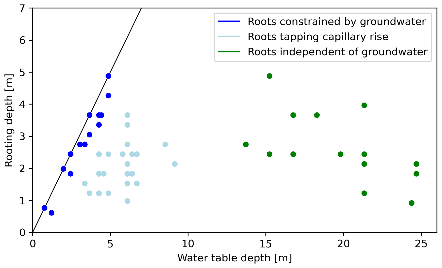
Figure 1 Illustration of the effect of water table depth on plant water uptake strategies, showing the rooting depth of 47 trees in eastern Nebraska plotted against water table depth measured at their specific sites. Soil and climate properties are relatively constant in the region. The roots can be divided into three distinct categories: (1) root growth is restricted by the groundwater, (2) roots are tapping the capillary rise, and (3) roots are independent of the groundwater. Data from Sprackling and Read (1979) and interpretation adapted from Fan et al. (2017).

At the local scale, the effect of the water table on plant growth has been studied extensively. In a large case study, in an area with similar soil and climate properties (Sprackling and Read, 1979), roots were found to fall into three categories (see Fig. 1): (1) roots terminating at or constrained by the groundwater, (2) roots tapping capillary rise and/or the groundwater in the wet periods and (3) roots completely detached from the groundwater (Fan et al., 2017). At the farm scale, these patterns were also observed (Zipper et al., 2015), with the conclusion that optimal plant growth occurs at the interface between the groundwater, limiting root respiration and roots being completely decoupled from the groundwater. In other words: the local optimum in vegetation growth lies where the best balance between water availability and (thermally controlled) evaporative demand is found.

Site-based studies suggest that, at the landscape scale, rooting depth depends on the climate in the uplands but on the water table depth in the lowlands (exceptions occur for various reasons, such as slope instability, insufficient soil depth and the presence of hardpans in the soil), presenting an optimal position where growth is aided by the groundwater while not suffering from rooting space limitation (Zipper et al., 2015; Fan et al., 2017). In global-scale analyses a similar picture arises, with vegetation growth being energy limited in high-altitude (Körner and Paulsen, 2004) and high-latitude regions (Keenan and Riley, 2018). Koirala et al. (2017) recently presented the first global study on the influence of the water table depth on vegetation growth. They found that both mechanisms, plant growth aided by groundwater in water-limited areas and plant growth hindered by groundwater due to oxygen stress, were reflected in the global satellite imagery analysis. The questions that remain are what the interplay is between climate-driven water and energy availability and groundwater for vegetation growth, how landscape position determines this interplay over different climates, and how extensive the area is in which vegetation growth is influenced by the groundwater.

Therefore, the purpose of this study is to understand and evaluate the global distribution of the effect of both climate-driven water and energy availability (reflected by humidity) and land drainage (reflected by water table depth) on vegetation growth and to assess the control of climate and landscape on these processes. To do this, we make use of global high-resolution (30 arcsec) datasets of water table depth, precipitation, potential evapotranspiration and tree growth, approximated by the fraction of absorbed photosynthetically active radiation (fAPAR). The relatively high resolution for a global study allows us to account for landscape-scale features within computational limits (Fan et al., 2017). We focus on trees, rather than vegetation in general, because they better represent the long-term local hydrologic regime. At the same time this lets us avoid confounding signals such as irrigation of annual crops, the response of annual vegetation to seasonal availability of soil water and inter-annual variation. In this way we aim to evaluate plant productivity over a climate gradient at the global scale and quantify the global extent of vegetation growth influenced by the water table.

2 Materials and methods

2.1 Input data

To approximate tree growth we used two different datasets. The first one is the MODIS fAPAR product, which is used as an approximation of plant primary production (Wu et al., 2010). The data have a 15 arcsec spatial and an 8 d temporal resolution (Myneni et al., 2015). For this study, we averaged the data over the period 2003 to 2018 and subsequently downsampled them to a spatial resolution of 30 arcsec using bilinear interpolation (see Fig. S1 in the Supplement). The second dataset is a global map of tree height, created from space-borne LIDAR images and validated against field measurements at different FLUXNET sites (see Fig. S2) (Simard et al., 2011). To solely focus on trees (to largely avoid the distorted signal of irrigated croplands), the fAPAR dataset was filtered with the tree height data, using a height threshold of 3 m. The resulting pixels are subsequently referred to as forest but might not in all regions be consistent with the classical understanding of forested ecosystems. For water table depth (WTD), the dataset by Fan et al. (2017) is used (updated version of the original dataset in Fan et al., 2013). This dataset was produced by an integrated groundwater, soil water and plant root uptake model at 30 arcsec resolution and at hourly time steps (see Fig. S3). The precipitation data (WorldClim V2) were created by interpolating station observations using ancillary information under MODIS land surface temperature and a digital elevation model (Fick and Hijmans, 2017) (see Fig. S4). As described in the introduction, temperature plays a major role in vegetation growth, both by reducing plant-available water with evaporative demand as well as by direct thermal control on growth. Here we focus on the hydrologic control on growth and account for the effect of temperature on water availability by normalising precipitation by (Penman–Monteith) potential evapotranspiration (PET), often referred to as humidity (the inverse of aridity). The data on potential evapotranspiration were produced from the data available in the WorldClim V2 database (see Figs. S5 and S6 for a global representation of PET and P∕PET respectively) (Zomer et al., 2008; Trabucco and Zomer, 2018). Although we focus on the hydrologic drivers, the direct control on growth exerted by temperature will be implicitly represented in one of the ecohydrological classes presented below. A summary of the datasets is provided in Table 1. It should be noted that both the WTD and fAPAR datasets were created using the MODIS MCD15A2H data and are therefore not completely independent. The MODIS data were used in the WTD model to describe the vegetation characteristics and to calculate the evapotranspiration and groundwater recharge fluxes. We believe this dependence to reflect the natural relation between vegetation and groundwater. Also, the impact on pixel-to-pixel correlations (between the fAPAR and WTD data) will be limited because of spatial exchange of information in the WTD dataset, which causes the WTD to mainly reflect topography rather than local vegetation conditions.

Myneni et al. (2015)Simard et al. (2011)Fan et al. (2017)Fick and Hijmans (2017)Trabucco and Zomer (2018)Beck et al. (2018)

Table 1 Summary of the datasets used in this study. The time period column describes the time frame of the input data of the specific studies to generate the datasets used here.

2.2 Analysis procedure

To understand and visualise the relation between the hydrologic gradients and forest growth, the local Pearson correlation was calculated between (1) WTD and fAPAR and between (2) P∕PET and fAPAR. This was done by applying a moving window (15×15 grid cells) to both datasets and correlating the values within that window. Windows containing less than 25 % of the data were discarded. This approach was chosen over catchment binning, as used in previous studies (Koirala et al., 2017), to minimise compensation of contrasting relations (rooting space limitation in lowlands and groundwater convergence-driven vegetation growth in uplands, both occurring in a single catchment and resulting in a net neutral relation between the water table and vegetation growth). Finally, each pixel contains a correlation value between the hydrologic gradient (WTD, P∕PET) and vegetation growth. With this approach it is assumed that within each window, ecosystems (e.g. forest age), soils (e.g. nutrient availability), management parameters (e.g. fertilisation), uncertainty in the input data and translation from fAPAR values to photosynthetic activity are homogeneous. The resulting correlation values are subsequently tested for significance, resulting in a negative, neutral or positive category in each pixel. The threshold of significance was calculated by casting the correlation values into the t-distribution with Eq. (1), in which r corresponds to the correlation, t to the t-value and df to the degrees of freedom.

$$\begin{array}{}\text{(1)}& t=r\sqrt{{\displaystyle \frac{\text{df}}{\mathrm{1}-r^{\mathrm{2}}}}}\end{array}$$

This can be rewritten to calculate the critical correlation value based on the t-value.

$$\begin{array}{}\text{(2)}& r={\displaystyle \frac{t}{\sqrt{\text{df}+t^{\mathrm{2}}}}}\end{array}$$

The degrees of freedom are determined with the following formula, in which n represents the number of samples.

$$\begin{array}{}\text{(3)}& \text{df}=(\mathrm{1}-{\text{df}}_{\text{offset}})n-\mathrm{2}\end{array}$$

The df_offset parameter is introduced to compensate for the spatial dependence of the samples due to the spatial organisation of the landscape. If the data were not auto-correlated, the df_offset parameter would be 0, in which case the traditional formula for calculating the confidence boundaries for correlation values appears. This additional parameter is determined by matching the significance boundaries of the t-test with boundaries determined by applying a permutation test and a bootstrap analysis (as described in Rahman and Zhang, 2016) to all windows with exactly 225 data points. The exact procedure and results, including a visual comparison of all three methods, are presented in Sect. S1 in the Supplement (see Figs. S7 and S8 for the results of the permutation test and bootstrapping analysis and the effect of the chosen metric on the final classification as described below). Subsequently, using the percent point function of the t-distribution with a significance level of p<0.05 (using a one-tailed approach), the significant t-value can be calculated. Feeding this value into Eq. (2), the t-value can be translated into the threshold correlation value. With 225 sample points (15×15-pixel moving window approach, assuming all pixels contain values), this yields significant correlation values above 0.121 for the correlations between P∕PET and fAPAR and 0.130 for the correlations between WTD and fAPAR (see Fig. S7). In windows containing fewer data points, this threshold increases accordingly. If an absolute correlation value exceeds the respective threshold, it is interpreted as significantly positive or negative, depending on the sign of the value.

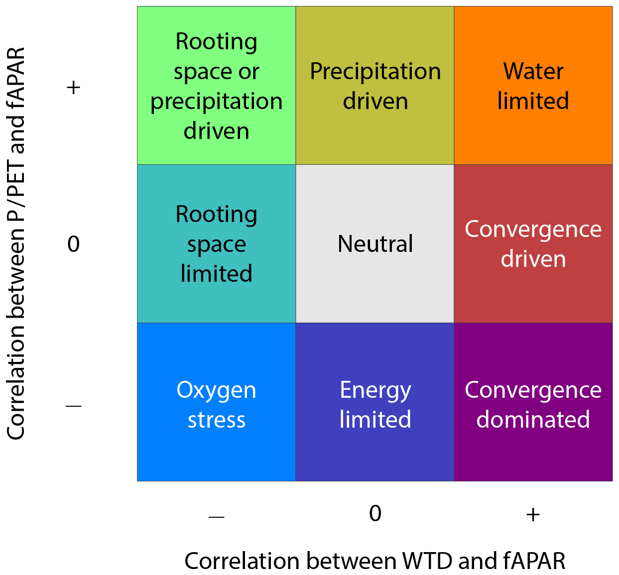
To investigate the interplay between P∕PET and WTD on forest growth, we combined the two significance maps, yielding nine distinctive classes (see Fig. 2), henceforth called ecohydrological classes. This combination is visualised using a bivariate colour scheme (Teuling et al., 2011; Speich et al., 2015). For the interpretation of the classes it needs to be considered that WTD is defined negatively; a higher value (less negative) corresponds to a shallower water table. Consequently a positive correlation between WTD and fAPAR means higher plant productivity with a shallower water table. A negative correlation signifies an increase in productivity for a deeper water table. A positive correlation between P∕PET and fAPAR means higher plant productivity with higher climate-driven water availability. To interpret the different classes, the key shown in Fig. 2 is proposed, which is discussed in the next section. The classes have been interpreted and named a priori, based on a review of the literature (see Introduction) and the current state of understanding.

The effect of landscape and climate on the hydrologic controls of vegetation growth was characterised by analysing the obtained ecohydrological classes in different climate zones and landscape positions. A recent, high-resolution Köppen–Geiger climate classification was used based on the same precipitation data as used for this study (Beck et al., 2018) (Fig. S9). To assess landscape positions, we used a landscape classification based on the moving window mean and standard deviation of WTD (5×5 pixels). Subsequently, the result was binned into seven landscape classes: wetland and open water, lowland, undulating, hilly, low mountainous, mountainous, high mountainous (see Sect. S2). The classification scheme is depicted in Fig. S10 and the resulting map is presented in Fig. S13. The resulting classification has been visually validated against several sample regions (Fig. S11 and S12).

All maps are downsampled to a resolution of 5 arcmin by applying a majority kernel on categorical and a mean kernel on continuous data. This was done to ease calculation and to be able to focus on the global patterns. Some figures are displayed at their full resolution to discern finer patterns in the maps, in which case this is stated in the caption.

2.3 Ecohydrological classes

Based on the significance of the correlation analysis between WTD and fAPAR and between P∕PET and fAPAR, we distinguish nine ecohydrological classes. These are depicted in Fig. 2. Below we provide a description of each class, discussing processes that might play a role in the vegetation–hydrologic gradient relation, starting from the bottom left.

Figure 2 Ecohydrological classes and their interpretation of the combined spatial correlation maps between respectively WTD, P∕PET and fAPAR. The figure is used as the legend of Figs. 3–7.

• Oxygen stress: in this class, negative correlations with both hydrologic gradients suggest that plant growth is limited by higher precipitation and shallower groundwater, indicating an excess of water with poor drainage conditions. This combination causes root-zone water logging, which limits root respiration (oxygen stress) and hence growth (Nosetto et al., 2009; Rodríguez-González et al., 2010; Florio et al., 2014; Zipper et al., 2015).

• Rooting space limited: here, plant growth is limited by shallower groundwater. In humid climates this indicates an excess of water in combination with poor drainage conditions. This class is largely similar to Oxygen stress except that there is no clear relation between precipitation and vegetation growth, which might be caused by the absence of a clear precipitation gradient. In arid and seasonally arid climates, the negative influence of the vicinity of the water table might be explained by high salt concentrations of the water in low landscape positions. Due to groundwater convergence, salts are transported to the lowest positions in the landscape, and high evapotranspiration increases the salt concentration dramatically, hindering plant growth (Jolly et al., 2008).

• Rooting space or precipitation driven: this class is a transitional class between Rooting space limited and Precipitation driven. Either the negative correlation between WTD and fAPAR (rooting space limitation) or the positive correlation between P∕PET and fAPAR (water limitation) explains the local tree growth gradients, while the other correlation is caused by a negative relation between WTD and precipitation. Often this negative relation can be explained by orography. Since WTD is roughly the inverse of altitude, locations with orographic precipitation (Fick and Hijmans, 2017) have a clear negative gradient between WTD and P. This negative correlation can sometimes also be explained by micro-climatic phenomena. This class can be interpreted as Rooting space limited if roots reach the groundwater and Precipitation driven if roots do not reach the groundwater. Alternatively, in the drier parts of the world, this class can also be interpreted directly as forests growing on the edges of basins where both a deeper water table and higher (orographic) precipitation help to counter growth limitation by high salt concentrations. In the centre of these basins the salt concentration is very high due to groundwater convergence transporting the salts and strong evapotranspiration. Higher rainfall in combination with well-drained soils can flush away the salt, creating more favourable conditions. This explains both the negative correlation between WTD and fAPAR and the positive correlation between P∕PET and fAPAR.

• Precipitation driven: plant growth is enhanced by increasing precipitation and is decoupled from the groundwater table. This likely occurs in well-drained, upland positions, where roots cannot reach the groundwater, under climatic conditions where plant growth is slightly to severely limited by water availability. Here, precipitation is the main driver of productivity.

• Water limited: plant growth is stimulated by a shallower water table and higher precipitation, indicating a general lack of water. This likely occurs on mountain slopes where the water table is within root reach and in (semi-)arid climates where plants depend on deeper groundwater.

• Convergence driven: plant growth is stimulated by a shallower water table. This represents areas that receive water from surrounding, higher areas by lateral redistribution of the groundwater, as described in Fan (2015). This likely occurs in arid or seasonally arid climates where precipitation is low and irregular but where the groundwater is within the reach of roots. These circumstances occur, for example, in desert oases and gallery forests (Fan, 2015). In mountainous regions this class can also be related to different processes that are linked to higher altitudes (further from the water table generally means higher in the landscape), like lower temperatures (Leal et al., 2007), a shorter growing season (Fan et al., 2009) and lower nutrient availability (Leuschner et al., 2007), that hamper tree growth.

• Convergence dominated: plant growth is stimulated by a shallower water table but is limited by an increase in precipitation. This class is a transition between Convergence driven and Energy limited. In water-limited climates this corresponds to similar environments as described in Convergence driven: vegetation growth is mainly determined by the gradient in water table depth. In energy-limited environments this class expresses higher vegetation growth in lower landscape positions (thus a positive correlation between WTD and fAPAR) as the energy availability is higher and the growing season longer. In both cases the negative correlation between precipitation and fAPAR mainly occurs because of the orographic link between the water table depth and precipitation.

• Energy limited: this class displays no significant relation between the proximity of the groundwater and plant growth, while plant growth is negatively influenced by humidity. The negative correlation with humidity indicates that vegetation growth is constrained by energy availability (here approximated by temperature), which is traditionally described as energy-limited systems. In lowland positions, this is caused by an imbalance in water availability and evaporative demand. A relative excess in plant-available water, as explained in Oxygen stress, limits root respiration and hence growth. In mountainous regions the negative relation between humidity and growth is directly caused by the temperature gradient as the highest landscape positions are colder and have a shorter growing season, reducing the growth potential. As the highest positions generally receive more precipitation and have lower potential evapotranspiration, the correlation between humidity and fAPAR is negative. The neutral correlation between WTD and fAPAR can be explained by vegetation being completely detached from the groundwater in mountainous areas and by the absence of a gradient in the water table in lowland positions.

• Neutral: this class contains the locations that show no significant correlation between either water table depth or precipitation and fAPAR.

Overall, there can be several process drivers in each ecohydrological class, dependent on climate and landscape position. In the next section, we will explore the global spatial distribution of the discussed ecoyhdrological classes.

3 Results

3.1 Global distribution of ecohydrological classes

Figure 3 displays the global distribution of the ecohydrological classes that were described in the previous section. In more than half of the pixels, forest growth is significantly influenced by the water table depth, and in more than 75 % by (normalised) precipitation, confirming the hypothesis that climate is an important but not the only driver of forest growth. All different classes are present in this global analysis to a varying degree on all continents and in all climate zones. Clear cases of water limitation (both correlations positive) are relatively under-represented as most water-limited areas were filtered out by applying a tree height threshold of 3 m. The results show that the water table depth plays a major role in determining forest growth, even in regions that are traditionally seen as energy-limited environments. WTD clearly shows a different signal than P∕PET, since the correlation between the two gradients can both be strongly positive (more precipitation with a shallower water table) or negative (more precipitation with a deeper water table, likely caused by orography) (see Fig. S16).

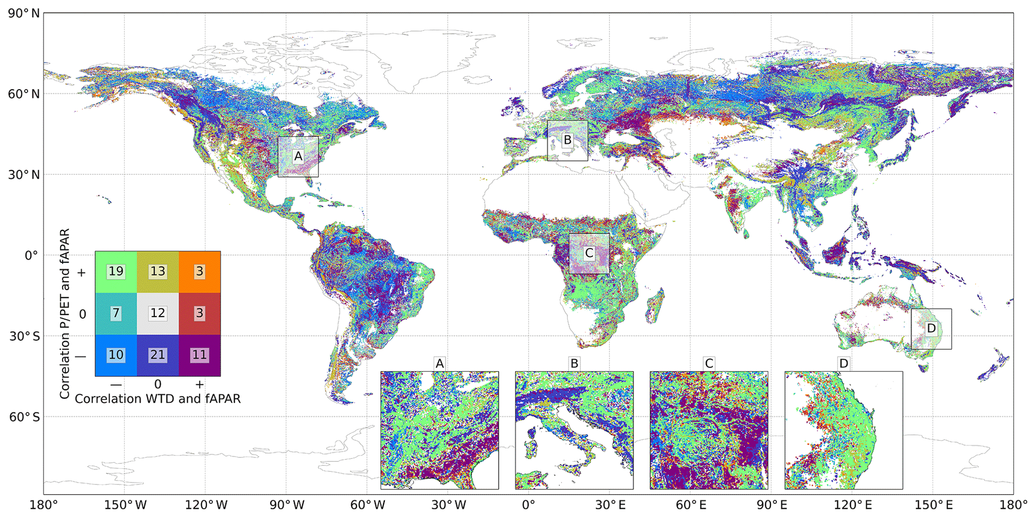
Figure 3 Global distribution of ecohydrological classes. The legend indicates the percentage of grid cells in the different classes. The map is downsampled to a resolution of 5 arcmin. For a bigger version of the map, see Fig. S17. Note that the percentages add up to 99, which is caused by rounding.

Four insets (15^∘) are displayed in Fig. 3. The same insets are displayed in Figs. S18 to S21 together with the input and individual correlation data. Inset A (Fig. S18) shows the Mississippi River valley on the left and the southern part of the American eastern coast on the right. The river valley itself shows a neutral or negative correlation between both WTD and P∕PET with fAPAR, representing an environment where too much water leads to over-saturation and water logging, which hampers tree growth. This corresponds to the ecohydrological classes Oxygen stress and Rooting space limited. Further away from the river, the relation between humidity and fAPAR changes to positive, leading to a classification of Rooting space or precipitation driven, which links a higher position in the landscape to more precipitation and more vegetation growth. Towards the coast, on the border between Georgia, Alabama and Florida, forest growth is Convergence dominated and in some places Water limited and Convergence driven.

Inset B (Fig. S19) shows south-eastern Europe with the Alps. In this mountainous region, plant growth is predominantly detached from groundwater influences (hardly any significant correlations between WTD and fAPAR). In the southern part of the Alps, forest growth is precipitation driven, while the northern part falls into the Energy limited class, featuring a negative correlation between P∕PET and fAPAR. In mountainous regions this class corresponds to an ecosystem that is detached from the groundwater and grows best in the lower- or mid-landscape positions. Higher up in the mountains, vegetation growth is disturbed by factors such as low temperatures, shallow soils and a reduced growing season. The hilly regions around the Alps are predominantly classified as Rooting space or precipitation driven, as in inset A. This corresponds to enhanced tree growth in the higher locations, associated with more rain and more rooting space. Another interesting feature in this inset is the Pannonian Basin (north-east in the inset), showing a similar pattern to the Mississippi valley of Rooting space limited vegetation growth. Groundwater convergence from the surrounding higher regions causes very shallow water table depths in this area, hampering forest growth.

Inset C (Fig. S20) depicts the Congo River basin. The Congo River and its side channels show similar patterns of increased vegetation growth on levees, leading to a Rooting space or precipitation driven classification. The regions to the south and east of the Congo River basin are dominated by savannas. These savannas receive a substantial amount of precipitation yearly, but rainfall is not evenly distributed over the year and makes water relatively scarce in comparison with the energy input at these latitudes (Verhegghen et al., 2012), leading to a classification of Convergence dominated. Areas at high altitude in this closeup show an Energy limited class; most forest growth occurs at the foot of mountains or on the slopes, while higher locations are less suitable due to lower temperatures and a shorter growing season.

Inset D (Fig. S21) shows an orographic region in eastern Australia, where vegetation growth is driven by the precipitation gradient. The lowland, west of the mountain range (Great Dividing Range), is classified as Rooting space limited and Rooting space or precipitation driven. Converging water from the mountain range causes a shallow water table depth in this region, hampering forest growth. The most western part of this inset that still contains trees receives between 250 and 500 mm precipitation per year. This region is Convergence driven, where vegetation depends on water from the higher areas.

All four insets display a high spatial variability in ecohydrological classes, demonstrating that the local interplay in climate and landscape position highly influence which hydrologic driver stimulates or hampers forest growth.

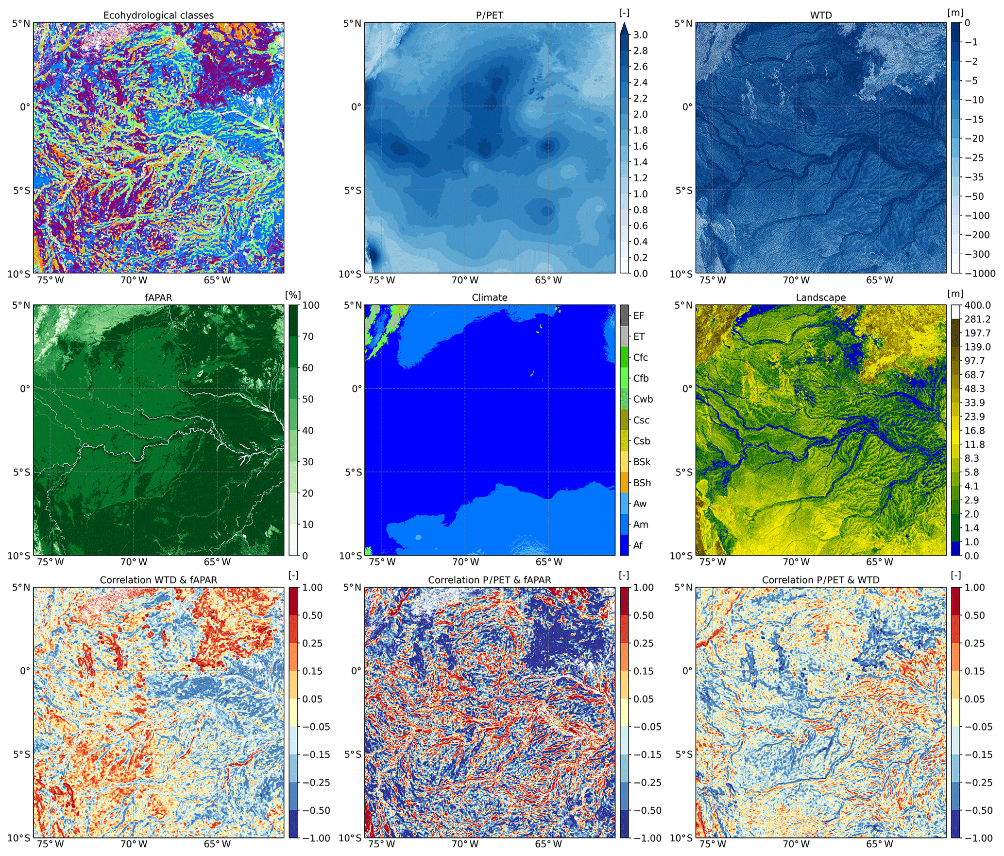
Figure 4 High-resolution illustration of ecohydrological classification in the Amazon. Input and correlation maps are shown at the full resolution of 30 arcsec. The white pixels in the upper left map (ecohydrological classes) represent the locations where the correlations were not calculated due to the tree height falling below the threshold value of 3 m.

3.2 Local examples at high resolution

To better visualise and understand the patterns of ecohydrological classes, detailed maps of the input, correlation and output maps are displayed in Figs. 4 and 5. Landscape position is approximated and displayed based on the standard deviation of the WTD map (which is the main constituent of the landscape classification procedure). This representation was chosen over the landscape classes, used throughout the rest of the paper, to obtained a more detailed visualisation.

The presented patterns in Fig. 4, displaying the western Amazon, show a clear overlap with ecosystem functioning as described in Ferreira-Ferreira et al. (2014). The river and its major contributing streams display the Rooting space or precipitation driven class. Considering the (slightly) negative correlation between WTD and P∕PET, this can be attributed to rooting space limited growth: the vegetation on the natural levees next to the channels is known for the highest and most diverse forests of the Amazon (High Varzea in Ferreira-Ferreira et al., 2014). On these levees the trees have more rooting space, receive more precipitation and suffer comparatively little from the inundation that characterises these rivers, leading to optimal growth conditions. In the depressions between streams (especially on the eastern side of these maps), forest growth is classified as Oxygen stress. Here forests suffer from the very frequent inundations that hamper their respiration. These same areas feature a positive relation between P∕PET and WTD, linking precipitation to percolation and a higher groundwater table.

The western parts of the maps show Convergence dominated forest growth. This area is higher than the eastern part, presenting fewer streams, and has a (slightly) higher relief, making inundation much rarer. This area agrees with the mapping of the white-sand ecosystems as published by Adeney et al. (2016). These ecosystems have sandy, very well-draining soils. Even slightly elevated surfaces know temporary periods of drought with lower vegetation growth. Tree growth in the lowest positions in these landscapes is higher, causing the Convergence dominated classification. In the hilly, north-eastern parts of the maps forest growth is also classified as Convergence dominated as well as Water limited, which is in stark contrast to the general perception of water abundance for vegetation growth in the Amazon region. This can be explained by the high amount of available energy, even with respect to such extensive amounts of rainfall. At the foot of these hilly regions vegetation can reach the groundwater and consequentially grow faster, thus causing a Convergence dominated classification. If the vegetation in a whole window cannot reach the groundwater anymore, this turns into the Water limited class.

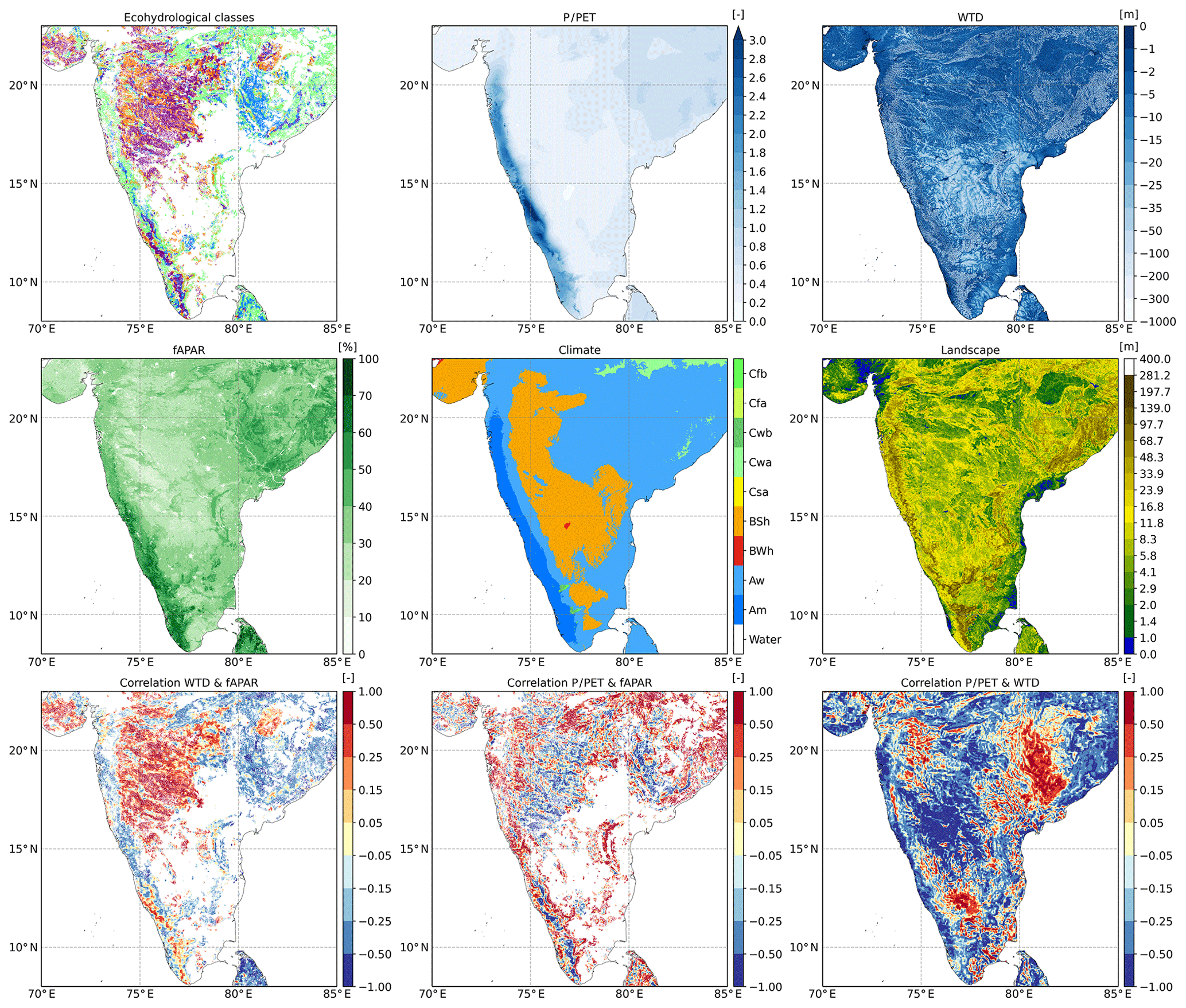
Figure 5 High-resolution illustration of ecohydrological classification over the Indian peninsula. Input and correlation maps are shown at the full resolution of 30 arcsec. The white pixels in the upper left map (ecohydrological classes) represent the locations where the correlations were not calculated due to the tree height falling below the threshold value of 3 m.

The second high-resolution example (Fig. 5) shows the Indian peninsula. The western part of India features a mountain range (Western Ghats), which is a strong orographic zone, receiving moisture from the Arabian Sea (especially during the monsoon season). This zone is predominantly classified as Rooting space or precipitation driven. In contrast to the Amazon example, this class is caused here by the precipitation-driven vegetation (positive correlation P∕PET and fAPAR), as the groundwater is too deep to be reached by the vegetation. The negative correlation between the WTD and fAPAR is caused by the strong orographic gradient, with higher precipitation in higher areas (with a lower water table). This negative gradient can be seen in the lower right subplot of Fig. 5.

The mountain range taps most of the precipitable water from the atmosphere, creating a vast rain shadow to the east (climate classes BWh and BSh). This area can be subdivided into two different zones: a southern zone and a northern zone. Although they receive similar yearly amounts of precipitation, the northern zone contains many more forests than the southern zone (which is mainly filtered out in this analysis since vegetation height is mostly under the threshold value of 3 m). This stark difference can be attributed to the distance of the water table to the surface. As can be seen in the upper right subplot of Fig. 5, the southern zone has much deeper groundwater than the northern zone. The forest growth classification in the northern zone, following the same rationale, is Convergence driven, Convergence dominated and Water limited; forest growth is highest in the lowest landscape positions, with the easiest access to the groundwater as an additional water source. Further east the amount of precipitation rises again (around 81^∘ E and 18^∘ N). This area features higher topography but a relatively shallow water table (plateau). This combination causes tree roots to be constrained, leading to the Oxygen stress classification. In contrast, the Eastern Ghats (first mountain range of India seen from the Bay of Bengal) show ecohydrological classes Rooting space or precipitation driven and Energy limited, which are linked to the orographic effect and decrease in temperature and growing season at higher altitudes.

When zooming in even further on the Amazon basin (Fig. S22) and India (Fig. S23), the potential of this high-resolution analysis becomes apparent. In Fig. S22 individual levees and gullies can be identified based on the ecohydrological classes, demonstrating local differences in water availability for forest growth. In Fig. S23 the strong gradients of the orographic effect and the driving effect of groundwater proximity as an alternative water source can be observed.

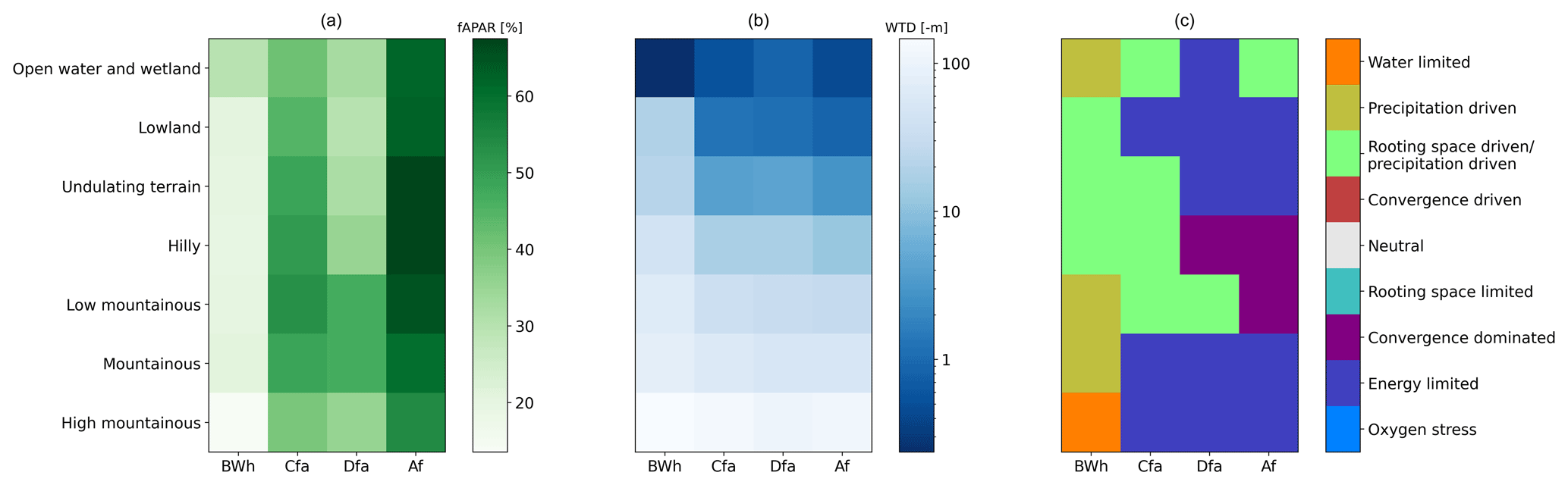
Figure 6 Distribution of average ecohydrological class as a function of landscape position and climate. This figure shows a subset of the Köppen–Geiger climates for clarity, namely arid (BWh), temperate (Cfa), continental (Dfa), and tropical (Af). For an extended version containing all the climates, see Figs. S24, S25 and S26. (a) Mean fAPAR, (b) mean water table depth and (c) prevalent ecohydrological class (after removing the cells in the neutral class). In Fig. S27 the full distribution of the ecohydrological classes within the selected climates is presented.

3.3 Landscape and climate as drivers of the hydrological controls

To characterise the influence of landscape and climate on the governing processes, the data have been segregated into Köppen–Geiger climate classes and landscape position classes. The results for four major climates are shown in Fig. 6. Figure 6a shows clear patterns in both landscape positions and climates. The arid climate (BWh) has much lower fAPAR values than the tropical climate (Af) and the intermediate temperate (Cfa) and continental (Dfa) climates fall in between, confirming the hypothesis that tree growth, at climate scale, follows the gradient of precipitation. Both extremes in the landscape (high mountainous and wetland) display lower fAPAR, except for the arid climate in which the lowest position in the landscape corresponds to the highest fAPAR. The highest fAPAR in the other climates falls in the intermediate landscape positions. Figure 6b shows mean water table depth in the different climate and landscape positions. As expected, the water table is generally deeper in arid climates compared to wetter climates in similar landscape positions, except for the lowest landscape position.

The ecohydrological classes (Fig. 6c) show some interesting patterns. In the lowest positions in the landscape, vegetation growth is limited by rooting space (in the arid class this becomes apparent in the full distribution of classes, as can be seen in Fig. S27 and can be linked to oases). Higher in the landscape we find a region where vegetation growth is driven by the precipitation gradient (Rooting space or precipitation driven and Precipitation driven). Rooting space or precipitation driven displays a negative correlation between WTD and fAPAR here as a consequence of more (orographic) precipitation at higher locations in the landscape. This process is similar in most climate zones (see Figs. 6c and S26), but the threshold within the landscape is lower in arid environments, following a general lower water table depth at similar landscape positions (Fig. 6b). Exceptions are the tropical climates (Af and Am), in which vegetation growth in mid-landscape positions is driven by groundwater convergence, hinting at a relative scarcity of water in comparison to the energy availability.

In the temperate, continental and tropical climates, where precipitation is generally high, limited rooting space in the lowest landscape positions suppresses growth. Consequentially, the optimum in fAPAR occurs higher up in the landscape, where rooting space is no longer a limitation. In the arid regions the lowest position in the landscape is favourable. This is associated with groundwater convergence from large areas, as water availability from precipitation is generally low. The highest landscape positions are classified as Energy limited in all but the arid climate, reflecting a strong thermal control on growth in mountainous regions. In the arid climate the mountainous regions are classified as Precipitation driven and Water limited, as water is scarce and vegetation is completely decoupled from the groundwater. Not surprisingly, the highest position in the arid climate has the lowest fAPAR of all landscape positions and climate regions. The continental climate (and even more strongly the boreal and arctic climates Dfc, Dsc and ET as can be seen in Fig. S26) is predominantly energy limited, as reflected by the Energy limited classification. In the low landscape positions this is linked to an excess in water availability with respect to the thermally controlled evaporative demand, while in the highest landscape positions vegetation growth is reduced by a low energy availability and a shorter growing season.

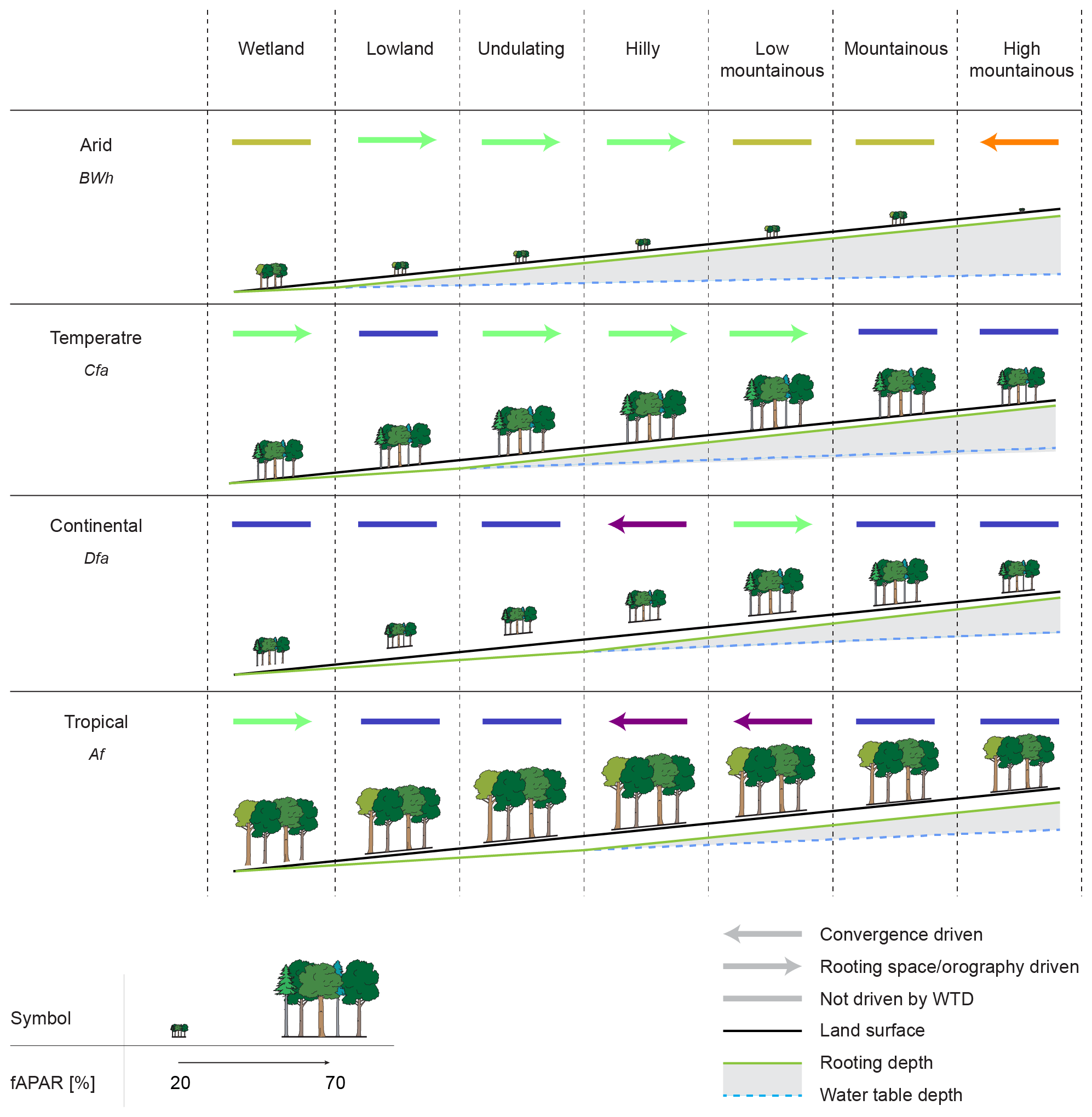
Figure 7 Conceptual framework summarising the links between fAPAR, water table depth, the correlations and implications for the patterns of rooting depth across climate and landscape classes. Different percentages of fAPAR are depicted as tree symbols, the ecohydrological classes are shown as arrows, where the colours represent the classes, and the point of the arrow indicates the sign of the correlation between WTD and fAPAR.

3.4 A novel framework to link forest growth to the hydrologic gradients in a climate–landscape continuum

Based on our results, we propose a framework for tree growth in different landscape positions and climates, displayed in Fig. 7. In arid regions the vegetation is concentrated in the lowest landscape positions, where roots can access the groundwater, which corresponds to the notion that vegetation in deserts predominantly thrives in oases, which are driven by groundwater convergence of extended areas. Another optimum, though with lower tree growth, exists higher up in the landscape, where the mountains are wetter, cooler and greener than the surrounding desert basins (better visible in Fig. 6a).

In the temperate and tropical climate, only one growth optimum is discernible. In the tropical climate this optimum corresponds to the region driven by local groundwater convergence (see Fig. 6a and c). This optimum lies exactly on the point where the correlation between water table depth and fAPAR switches from neutral/positive (see Fig. S27) to negative, implying the existence of a distance to the groundwater that is shallow enough to be accessible to roots and deep enough for it not to negatively influence root growth. In the temperate climate the optimum of vegetation growth lies in the zone classified as Rooting space or precipitation driven, with a negative correlation between WTD and fAPAR. In contrast to lower positions in the landscape, this zone displays a positive correlation with humidity, hinting at precipitation-driven vegetation, only displaying a negative correlation between WTD and fAPAR because higher precipitation falls at higher locations. This suggests that vegetation is detached from the groundwater in these mid-landscape positions, with vegetation growth being limited by water availability. In the lowest landscape positions even more water is available but, because the shallow groundwater confines the root zone, plants cannot take optimal advantage of the resource.

The continental climate shows a very similar pattern to the temperate and tropical climates, although fAPAR values are lower. This climate does show a second optimum in fAPAR in the lowest landscape position (better visible in Fig. 6a), similar to the arid climate. In most landscape positions in the continental climate vegetation is Energy limited, indicating a relative excess in plant-available water in the lowlands and thermally controlled growth in the highlands.

4 Discussion

4.1 Correlation in hydrologic gradients

The presented results show that global gradients of humidity and water table depth have a substantial effect on forest growth. These gradients, however, are not independent, which needs to be considered when interpreting the results. The correlation between P∕PET and WTD is shown in Fig. S16 and shows clear spatial patterns of both positive and negative values. A negative correlation corresponds to higher precipitation with a deeper water table, while a positive correlation indicates lower precipitation with a deeper water table. In terms of processes, these relations can best be explained when considering that water table depth is roughly the inverse of altitude (especially in hilly and mountainous terrain). A negative correlation between WTD and P∕PET would correspond to more precipitation higher in the landscape, which is linked to orographic precipitation. Positive correlation values between WTD and P seem to often occur in either low-lying areas, where more precipitation yields more percolation and a shallower water table, or in mountainous areas, which could correspond to a decrease in precipitation with altitude due to a loss of atmospheric moisture due to orographic precipitation in lower-lying areas. These processes are clearly present in the class Rooting space or precipitation driven, but a correlation between P∕PET and WTD should be considered in all other classes as well.

4.2 Variation over time

In this study we analysed forest growth under long-term average gradients of water table depth and normalised precipitation, even though both hydrologic gradients can show considerable seasonality. We acknowledge that seasonality in precipitation and water table depth can influence the local vegetation type, but we believe that by focusing on forests only, long-term averages in hydrologic gradients can provide useful insights. It can be assumed that forests are strongly adapted to the local hydrological regime and therefore mainly respond to long-term changes in these regimes. This approach was chosen to understand the global patterns of long-term ecosystem behaviour and water resources. By using the long-term average gradients, we focus on the question of whether and where forests are driven by the groundwater, precipitation, or both.

4.3 A start for a more sophisticated forest growth representation in global modelling studies

Many global Earth system modelling studies do not account for water table depth as a driver of forest growth. Our results suggest that landscape-scale interaction between vegetation and groundwater, including lateral convergence, moisture and oxygen stress, is important in most parts of the world and should be better represented in these Earth system models. Groundwater can either be an extra water source for vegetation growth but also a constraint on root growth and, with that, vegetation growth. The presented framework can serve as a first approach to account for both forest growth stimulation and growth limitation based on precipitation and water table depth in a climate–landscape continuum. Local examples, such as the Amazon River and the mainland of India, show a consistent overlap between the presented patterns and expected tree growth, based on the understanding of the ecosystems. It needs to be considered that seasonality and inter-annual variability of both precipitation and the water table can change the presented patterns substantially, but the understanding of average ecosystem behaviour on a climate–landscape continuum can be used as a baseline in further studies. The global importance of the landscape-scale water table variability for forest growth proves that it needs to be considered in global environmental modelling.

5 Conclusions

The goal of this study was to relate climate- and groundwater-driven water availability to forest growth on a global scale. The presented results show that across most of Earth's surface, water is an important control on plant productivity, determining the presence of vegetation and constraining its growth. Water table depth, an often ignored parameter in global Earth system modelling, displays a significant influence on vegetation growth in more than 50 % of the forested pixels, both positively (e.g. tree growth stimulation in oases) and negatively (e.g. tree growth hindrance in swamps). In a substantial part of the globe, this influence does not overlap with an influence of precipitation, although both gradients generally show a strong spatial correlation.

Inter-climate analysis demonstrates that, at the continental scale, vegetation growth is strongly driven by humidity; vegetation in wetter climates shows higher energy absorption. Within these climate zones, vegetation growth can substantially change over the landscape gradient. The effect of landscape is, however, not constant in all climate zones. As hypothesised, vegetation growth in arid regions is mainly driven by groundwater convergence, showing the highest energy absorption in the lowest landscape positions. In more humid climate zones, tree growth presents an optimum in mid-landscape positions. Below this optimum a shallow groundwater table limits root growth and vegetation development, while at and above this optimum vegetation is detached from the groundwater and tree growth mainly follows the precipitation gradient. At high altitude and in colder climates vegetation is mainly driven by energy availability. The proposed framework illustrates the importance of coupling landscape and climate together to describe vegetation patterns worldwide, tying root growth and water availability from precipitation and groundwater together. In the light of global changes in hydrologic gradients and land use, the water cycle will substantially change in the future. To predict the changes and mitigate the effects, water availability and root growth should be considered in global environmental modelling.