the Creative Commons Attribution 4.0 License.
the Creative Commons Attribution 4.0 License.
 | 24 Jan 2020
Inter-annual variability of the global terrestrial water cycle
Dongqin Yin
Michael L. Roderick
Variability of the terrestrial water cycle, i.e. precipitation (P), evapotranspiration (E), runoff (Q) and water storage change (ΔS) is the key to understanding hydro-climate extremes. However, a comprehensive global assessment for the partitioning of variability in P between E, Q and ΔS is still not available. In this study, we use the recently released global monthly hydrologic reanalysis product known as the Climate Data Record (CDR) to conduct an initial investigation of the inter-annual variability of the global terrestrial water cycle. We first examine global patterns in partitioning the long-term mean between the various sinks , and and confirm the well-known patterns with partitioned between and according to the aridity index. In a new analysis based on the concept of variability source and sinks we then examine how variability in the precipitation (the source) is partitioned between the three variability sinks , and along with the three relevant covariance terms, and how that partitioning varies with the aridity index. We find that the partitioning of inter-annual variability does not simply follow the mean state partitioning. Instead we find that is mostly partitioned between , and the associated covariances with limited partitioning to . We also find that the magnitude of the covariance components can be large and often negative, indicating that variability in the sinks (e.g. , ) can, and regularly does, exceed variability in the source (). Further investigations under extreme conditions revealed that in extremely dry environments the variance partitioning is closely related to the water storage capacity. With limited storage capacity the partitioning of is mostly to , but as the storage capacity increases the partitioning of is increasingly shared between , and the covariance between those variables. In other environments (i.e. extremely wet and semi-arid–semi-humid) the variance partitioning proved to be extremely complex and a synthesis has not been developed. We anticipate that a major scientific effort will be needed to develop a synthesis of hydrologic variability.
- Article
(5335 KB) - Full-text XML
-
Supplement
(4216 KB) - BibTeX
- EndNote


In describing the terrestrial branch of the water cycle, the precipitation (P) is partitioned into evapotranspiration (E), runoff (Q) and change in water storage (ΔS). With averages taken over many years, is usually assumed to be zero and it has long been recognized that the partitioning of the long-term mean annual precipitation () between and was jointly determined by the availability of both water () and energy (represented by the net radiation expressed as an equivalent depth of water and denoted ). Using data from a large number of watersheds, Budyko (1974) developed an empirical relation relating the evapotranspiration ratio () to the aridity index (). The resultant empirical relation and other Budyko-type forms (e.g. Fu, 1981; Choudhury, 1999; Yang et al., 2008; Roderick and Farquhar, 2011; Sposito, 2017) that partition P between E and Q have proven to be extremely useful in both understanding and characterizing the long-term mean annual hydrological conditions in a given region.
However, the long-term mean annual hydrologic fluxes rarely occur in any given year. Instead, society must (routinely) deal with variability around the long-term mean. The classic hydro-climate extremes are droughts and floods but the key point here is that hydrologic variability is expressed on a full spectrum of time and space scales. To accommodate that perspective, we need to extend our thinking beyond the long-term mean to ask how the variability of P is partitioned into the variability of E, Q and ΔS (e.g. Orth and Destouni, 2018).
Early research on hydrologic variability focussed on extending the Budyko curve. In particular, Koster and Suarez (1999) used the Budyko curve to investigate inter-annual variability in the water cycle. In their framework, the evapotranspiration standard deviation ratio (defined as the ratio of standard deviation for E to P, σE∕σP) was (also) estimated using the aridity index (). The classic Koster and Suarez framework has been widely applied and extended in subsequent investigations of the variability in both E and Q, using catchment observations, reanalysis data and model outputs (e.g. McMahon et al., 2011; Wang and Alimohammadi, 2012; Sankarasubramanian and Vogel, 2002; Zeng and Cai, 2015). However, typical applications of the Koster and Suarez framework have previously been at regional scales and there is still no comprehensive global assessment for partitioning the variability of P into the variability of E, Q and ΔS. One reason for the lack of a global comprehensive assessment is the absence of gridded global hydrologic data. Interestingly, the atmospheric science community have long used a combination of observations and model outputs to construct gridded global-scale atmospheric re-analyses and such products have become central to atmospheric research. Those atmospheric products also contain estimates of some of the key water cycle variables (e.g. P, E), such as in the widely used interim ECMWF Re-Analysis (ERA-Interim; Dee et al. 2011). Though efforts have been taken to develop land-based products from atmospheric reanalyses, e.g. ERA-Land (Balsamo et al., 2015) and MERRA-Land (Reichle et al., 2011) databases, the central aim of atmospheric re-analysis is to estimate atmospheric variables. That atmospheric-centric aim, understandably, ignores many of the nuances of soil water infiltration, vegetation water uptake, runoff generation and many other processes of central importance in hydrology.
Hydrologists have only recently accepted the challenge of developing their own re-analysis-type products with perhaps the first serious hydrologic re-analysis being published as recently as a few years ago (Rodell et al., 2015). More recently, the Princeton University group has extended this early work by making available a gridded global terrestrial hydrologic re-analysis product known as the Climate Data Record (CDR) (Zhang et al., 2018). Briefly, the CDR was constructed by synthesizing multiple in situ observations, satellite remote sensing products and land surface model outputs to provide gridded estimates of global land precipitation P, evapotranspiration E, runoff Q and total water storage change ΔS (, monthly, 1984–2010). In developing the CDR, the authors adopted local water budget closure as the fundamental hydrologic principle. That approach presented one important difficulty. Global observations of ΔS start with the GRACE satellite mission from 2002. Hence before 2002 there is no direct observational constraint on ΔS and the authors made the further assumption that the mean annual ΔS over the full 1984–2010 period was zero at every grid box. That is incorrect in some regions (e.g. Scanlon et al., 2018) and represents an observational problem that cannot be overcome. However, our interest is in the year-to-year variability and for that application, the assumption of no change in the mean annual ΔS over the full 1984–2010 period is unlikely to lead to major problems since we are not looking for subtle changes over time. With that caveat in mind, the aim of this study is to use this new 27-year gridded hydrologic re-analysis product to conduct an initial investigation of the inter-annual variability of the terrestrial branch of the global water cycle.
The paper is structured as follows. We begin in Sect. 2 by describing the various climate and hydrologic databases used in this study and also include a further assessment of the suitability of the CDR database for this initial variability study. In Sect. 3, we examine relationships between the mean and variability in the four water cycle variables (P, E, Q and ΔS). In Sect. 4, we first relate the variabilities to the classical aridity index and then use those results to evaluate the theory of Koster and Suarez (1999). Subsequently we examine how the variance of P is partitioned into the variances (and relevant covariances) of E, Q and ΔS and undertake an initial survey that investigates some of the factors controlling the variance partitioning. We conclude the paper with a discussion summarizing what we have learnt about water cycle variability over land by using the CDR database.
2.1 Methods
The water balance is defined by
with P the precipitation, E the evapotranspiration, Q the runoff and ΔS the total water storage change in time step t (annual in this study). By the usual variance law, we have
which includes all relevant variances (denoted σ2) and covariances (denoted cov). Equation (2) can be thought of as the hydrologic variance balance equation.
2.2 Hydrologic and climatic data
We use the CDR database (Zhang et al., 2018), which is a recently released global land hydrologic re-analysis. This product includes global precipitation P, evapotranspiration E, runoff Q and water storage change ΔS (, monthly, 1984–2010). In this study we focus on the inter-annual variability and the monthly water cycle variables (P, E, Q and ΔS) are aggregated to annual totals. The CDR does not report additional radiation variables and we use the NASA/GEWEX Surface Radiation Budget (SRB) Release-3.0 (monthly, 1984–2007, ) database (Stackhouse et al., 2011) to calculate Eo (defined as the net radiation expressed as an equivalent depth of liquid water, Budyko, 1974). We then calculate the aridity index () using P from the CDR and Eo from the SRB databases (see Fig. S1a in the Supplement).
In general, we anticipate two important factors, i.e. the water storage capacity and the presence of ice/snow at the surface, which are most likely to have influence on the partitioning of hydrologic variability. For the storage, the active range of the monthly water storage variation was used to approximate the water storage capacity (Smax). In more detail, the water storage S(t) at each time step t (monthly here) was first calculated from the accumulation of ΔS(t), i.e. , where we assumed zero storage at the beginning of the study period (i.e. S(0)=0). With the resulting time series available, Smax was estimated as the difference between the maximum and minimum S(t) during the study period at each grid box (see Fig. S1b in the Supplement). The estimated Smax shows a large range from 0 to 1000 mm with the majority of values from 50 to 600 mm (Fig. S1b), which generally agrees with global rooting depth estimates assuming that water occupies from 10 % to 30 % of the soil volume at field capacity (Jackson et al., 1996; Wang-Erlandsson et al., 2016; Yang et al., 2016). To characterize snow/ice cover, and to distinguish extremely hot and cold regions, we also make use of a gridded global land air temperature dataset from the Climatic Research Unit (CRU TS4.01 database, monthly, 1901–2016, ) (Harris et al., 2014) (see Fig. S1c in the Supplement).
2.3 Spatial mask to define study extent
The CDR database provides an estimate of the uncertainty (±1σ) for each of the hydrologic variables (P, E, Q, ΔS) in each month. We use those uncertainty estimates to identify and remove regions with high relative uncertainty in the CDR data. The relative uncertainty is calculated as the ratio of root mean square of the uncertainty (±1σ) to the mean annual P, E and Q at each grid box following the procedure used by Milly and Dunne (2002). Note that the long-term mean ΔS is zero by construction in the CDR database, and for that reason we did not use ΔS to calculate the relative uncertainty. Grid boxes with a relative uncertainty (in P, E and Q) of more than 10 % are deemed to have high relative uncertainty (Milly and Dunne, 2002) and were excluded from the study extent. The excluded grid boxes were mostly in the Himalayan region, the Sahara Desert and in Greenland. The final spatial mask is shown in Fig. S2 and this has been applied throughout this study.
2.4 Further evaluation of CDR data for variability analysis
In the original work, the CDR database was validated by comparison with independent observations including (i) mean seasonal cycle of Q from 26 large basins (see Fig. 8 in Zhang et al., 2018), (ii) mean seasonal cycle of ΔS from 12 large basins (Fig. 10 in Zhang et al., 2018), (iii) monthly runoff from 165 medium size basins and a further 862 small basins (Fig. 14 in Zhang et al., 2018), and (iv) summer E from 47 flux towers (Fig. 16 in Zhang et al., 2018). Those evaluations did not directly address variability in various water cycle elements. With our focus on the variability we decided to conduct further validations of the CDR database beyond those described in the original work. In particular, we focussed on further independent assessments of E and we use monthly (as opposed to summer) observations of E from FLUXNET to evaluate the variability in E. We also compare the evapotranspiration E in the CDR with two other gridded global E products that were not used to develop the CDR including the LandFluxEval database (, monthly, 1989–2005) (Mueller et al., 2013) and the Max Planck Institute database (MPI, , monthly, 1982–2011) (Jung et al., 2010). The runoff Q in the CDR is further compared with the gridded European Q product E-RUN (, monthly, 1951–2015) (Gudmundsson and Seneviratne, 2016a).
For the comparison to FLUXNET observations (Baldocchi et al., 2001; Agarwal et al., 2010) we identified 32 flux tower sites (site locations are shown in Fig. S3 and details are shown in Table S1) with at least 3 years of continuous (monthly) measurements using the FluxnetLSM R package (v1.0) (Ukkola et al., 2017). The monthly totals and annual climatology of P and E from CDR generally follow FLUXNET observations, with high correlations and reasonable root mean square error (Figs. S4–S5, Table S1). Comparison of the point-based FLUXNET (∼100 m–1 km scale) with the grid-based CDR (∼50 km scale) is problematic since the CDR represents an area that is at least 2500 times larger than the area represented by the individual FLUXNET towers and we anticipate that the CDR record would be “smoothed” relative to the FLUXNET record. With that in mind, we chose to compare the ratio of the standard deviation of E to P between the CDR and FLUXNET databases and this normalized comparison of the hydrologic variability proved encouraging (Fig. S6).
The comparison of E between the CDR and the LandFluxEval and MPI databases also proved encouraging. We found that the monthly mean E from the CDR database is slightly underestimated compared with the LandFluxEVAL database (Fig. S7a) but agrees closely with the MPI database (Fig. S8a). In terms of variability, the standard deviations of monthly E from the CDR are in very close agreement with the LandFluxEVAL database (Fig. S7c), but there is a bias and scaling offset for the comparison with the MPI database, particularly for the grid cells with low standard deviation of E (Fig. S8c). The comparison of runoff Q between the E-RUN and CDR databases shows that the two databases have very similar spatial patterns of both the long-term mean () and standard deviation (σQ) of the monthly Q (Fig. S10). The grid-by-grid comparison results are also encouraging, showing slight bias of both the long-term mean and standard deviation of monthly Q in the CDR database compared with the E-RUN database (Fig. S11).
We concluded that while the CDR database was unlikely to be perfect, it was nevertheless suitable for an initial exploratory survey of inter-annual variability in the terrestrial branch of the global water cycle.
3.1 Mean annual P, E and Q and the Budyko curve
The global pattern of mean annual P, E and Q using the CDR data (1984–2007) is shown in Fig. 1. The mean annual P () is prominent in tropical regions, southern China, and eastern and western North America (Fig. 1a). The magnitude of mean annual E () more or less follows the pattern of in the tropics (Fig. 1b) while the mean annual Q () is particularly prominent in the Amazon, South and Southeast Asia, tropical parts of western Africa, and in some other coastal regions at higher latitudes (Fig. 1c).

Figure 1Mean annual (1984–2010) (a) P, (b) E and (c) Q. Note that the mean annual ΔS in the CDR database is zero by construction and is not shown.
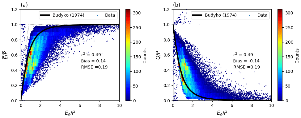
Figure 2Relationship of mean annual (a) evapotranspiration () and (b) runoff () ratios to the aridity index () from the CDR and SRB databases. For comparison, the Budyko (1974) curve is shown on panel (a). The curve on panel (b) is calculated assuming a steady state ().
We relate the grid-box level ratio of to in the CDR database to the classical Budyko (1974) curve using the aridity index () (Fig. 2a). As noted previously, in the CDR database, is forced to be zero and this enforced steady state (i.e. ) allowed us to also predict the ratio of to using the same Budyko curve (Fig. 2b). The Budyko curves follow the overall pattern in the CDR data, which agrees with previous studies showing that the aridity index can be used to predict water availability (e.g. Gudmundsson et al., 2016). However, there is substantial scatter due to, for example, regional variations related to seasonality, water storage change and the landscape characteristics (Milly, 1994a, b; Padrón et al., 2017). With that caveat in mind, the overall patterns are as expected, with following in dry environments () while follows in wet environments () (Fig. 2).
3.2 Inter-annual variability in P, E, Q and ΔS
We use the variance balance equation (Eq. 2) to partition the inter-annual into separate components due to , , along with the three covariance components [2cov(EQ), 2cov(E,ΔS), 2cov(Q,ΔS)] (Fig. 3). The spatial pattern of (Fig. 3a) is very similar to that of (Fig. 1a), which implies that the is positively correlated with . In contrast the partitioning of to the various components is very different from the partitioning of (cf. Figs. 1 and 3). First we note that while the overall spatial pattern of more or less follows , the overall magnitude of is much smaller than and in most regions, and in fact is also generally smaller than . The prominence of (compared to ) surprised us. The three covariance components [cov(E,Q), cov(E,ΔS), cov(Q,ΔS)] are also important in some regions. In more detail, the cov(E,Q) term is prominent in regions where is large and is mostly negative in those regions (Fig. 3e), indicating that years with lower E are associated with higher Q and vice versa. There are also a few regions with prominent positive values for cov(EQ) (e.g. the seasonal hydroclimates of northern Australia) indicating that in those regions, years with a higher E are associated with higher Q. The cov(E,ΔS) term (Fig. 3f) has a similar spatial pattern to the cov(E,Q) term (Fig. 3e) but with a smaller overall magnitude. Finally, the cov(Q,ΔS) term shows a more complex spatial pattern, with both prominent positive and negative values (Fig. 3g) in regions where (Fig. 3c) and (Fig. 3d) are both large.
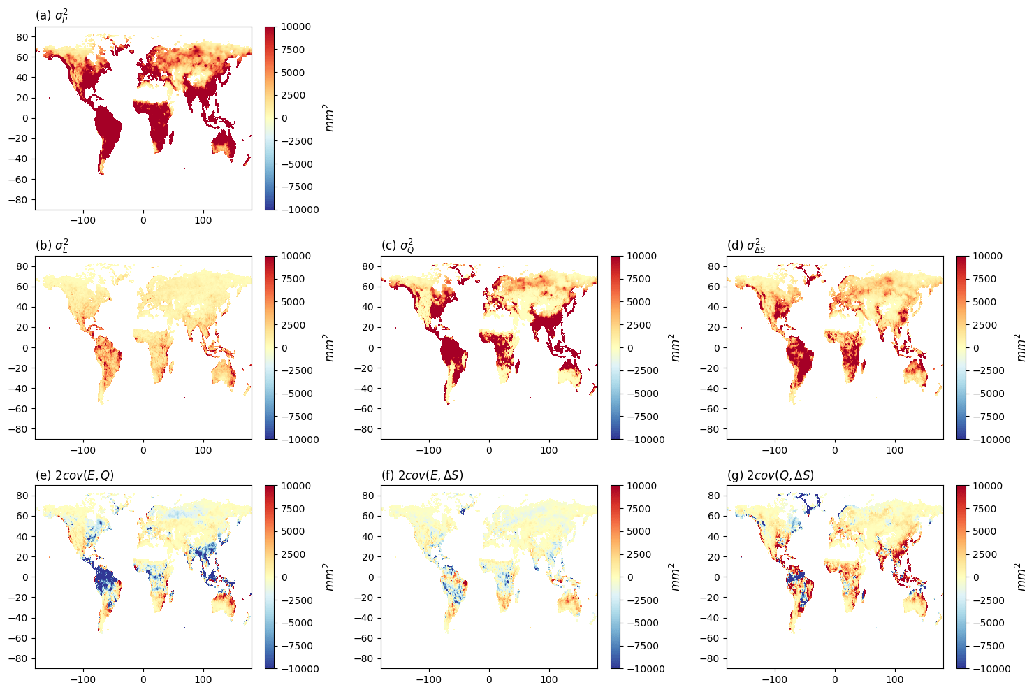
Figure 3Water cycle variances (, , , ) and covariances [cov(EQ), cov(E,ΔS), cov(Q,ΔS)]. Note that we have multiplied the covariances by two (see Eq. 2).
These results show that the spatial patterns in variability are not simply a reflection of patterns in the long-term mean state. On the contrary, we find that of the three primary variance terms, the overall magnitude of (inter-annual) is the smallest, implying the least (inter-annual) variability in E. This is very different from the conclusions based on spatial patterns in the mean P, E and Q (see Sect. 3.1). Further, while more or less follows as expected, we were surprised by the magnitude of which, in general, substantially exceeds the magnitude of . Further, the magnitude of the covariance terms can be important, especially in regions with high . However, unlike the variances, the covariance can be both positive and negative and this introduces additional complexity. For example, with a negative covariance it is possible for the variance in Q () to exceed the variance in P (). To examine that in more detail we calculated the equivalent frequency distribution for each of the plots in Fig. 3. The results (Fig. S9) further emphasize that in general, is the smallest of the variances (Fig. S9b). We also note that the frequency distributions for the covariances (Fig. S9e, f, g) are not symmetrical. In summary, it is clear that spatial patterns in the inter-annual variability of the water cycle (Fig. 3) do not simply follow the spatial patterns for the inter-annual mean (Fig. 1).
3.3 Relation between variability and the mean state for P, E, Q
Differences in the spatial patterns of the mean (Fig. 1) and inter-annual variability (Fig. 3) in the global water cycle led us to further investigate the relation between the mean and the variability for each separate component. Here we relate the standard deviation (σP, σE, σQ) instead of the variance to the mean of each water balance flux (Fig. 4) since the standard deviation has the same physical units as the mean, making the results more comparable. As inferred previously, we find σP to be positively correlated with but with substantial scatter (Fig. 4a). The same result more or less holds for the relation between σQ and (Fig. 4c). In contrast the relation between σE and is very different (Fig. 4b). In particular, σE is a small fraction of and this complements the earlier finding (Fig. 4b) that the inter-annual variability for E is generally smaller than for the other physical variables (P, Q and ΔS). (The same result was also found using both LandFluxEVAL and MPI databases; see Fig. S12 in the Supplement.) Importantly, unlike P and Q, E is constrained by both water and energy availability (Budyko, 1974) and the limited inter-annual variability in E presumably reflects limited inter-annual variability in the available (radiant) energy (Eo). This is something that could be investigated in a future study.
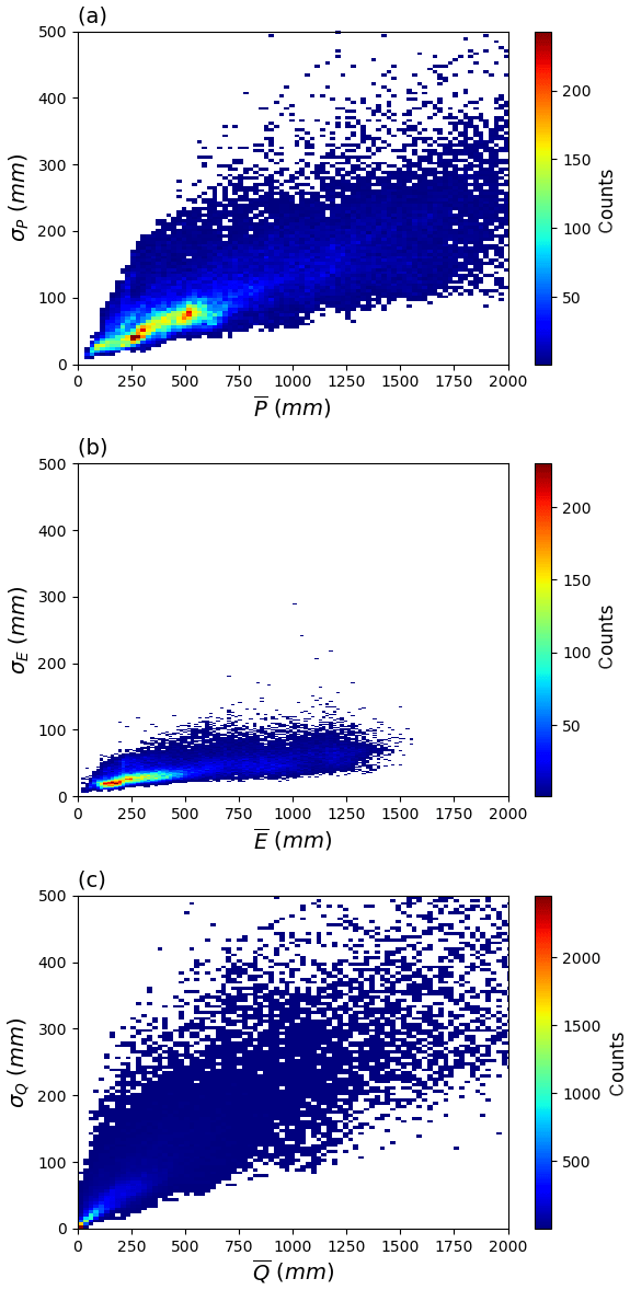
Figure 4Relation between inter-annual mean and standard deviation for (a) P, (b) E and (c) Q from the CDR database. Note that the mean annual ΔS is zero by construction and is not shown.
In the previous section, we investigated spatial patterns of the mean and the variability in the global water cycle. In this section, we extend that by investigating the partitioning of to the three primary physical terms (, , ) along with the three relevant covariances. For that, we begin by comparing the Koster and Suarez (1999) theory against the CDR data and then investigate how the partitioning of the variance is related to the aridity index (see Fig. S1a in the Supplement). Following that, we investigate variance partitioning in relation to both our estimate of the storage capacity Smax (see Fig. S1b in the Supplement) as well as the mean annual air temperature (see Fig. S1c in the Supplement) that we use as a surrogate for snow/ice cover. We finish this section by examining the partitioning of variance at three selected study sites that represent extremely dry/wet, high/low water storage capacity and the hot/cold spectrums.
4.1 Comparison with the Koster and Suarez (1999) theory
We first evaluate the classical empirical curve of Koster and Suarez (1999) by relating ratios σE∕σP and σQ∕σP to the aridity index (Fig. 5). The ratio σE∕σP in the CDR database is generally overestimated by the empirical Koster and Suarez curve, especially in dry environments (e.g. ) (Fig. 5a). The inference here is that the Koster and Suarez theory predicts σE∕σP to approach unity in dry environments while the equivalent value in the CDR data is occasionally unity but is generally smaller. With σE∕σP generally overestimated by the Koster and Suarez theory we expect, and find, that σQ∕σP is generally underestimated by the same theory (Fig. 5b). The same overestimation was found based on the other two independent databases for E (LandFluxEVAL and MPI) (Fig. S13). This overestimation is discussed further in Sect. 5.
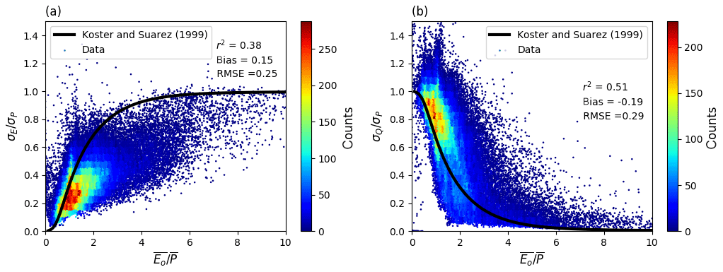
Figure 5Relationship of inter-annual standard deviation of (a) evapotranspiration (σE∕σP) and (b) runoff (σQ∕σP) ratios to aridity (). The curves represent the semi-empirical relations from Koster and Suarez (1999).
4.2 Relating inter-annual variability to aridity
Here we examine how the fraction of the total variance in precipitation accounted for by the three primary variance terms along with the three covariance terms varies with the aridity index () (Fig. 6). (Also see Fig. S14 for the spatial maps.) The ratio is close to zero in extremely wet regions and has an upper limit noted previously (Fig. 5a) that approaches unity in extremely dry regions (Fig. 6a). The ratio is close to zero in extremely dry regions but approaches unity in extremely wet regions but with substantial scatter (Fig. 6b). The ratio is close to zero in both extremely dry/wet regions (Fig. 6c) and shows the largest range at an intermediate aridity index ().
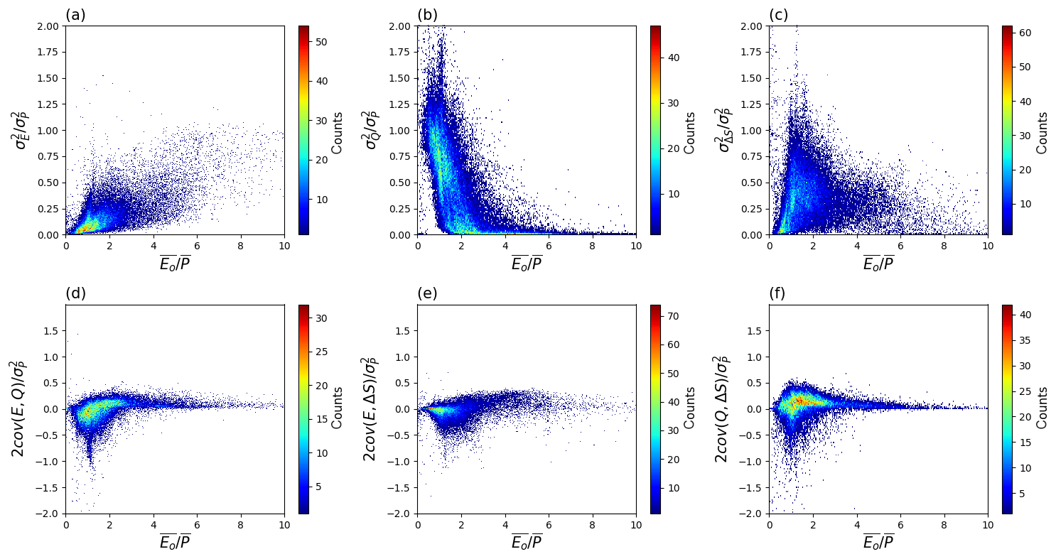
Figure 6Relation between water cycle variances and covariances (see Fig. 3b–g) as a fraction of the variance of P () and the aridity index () coloured by density. Note that we have multiplied the covariance components by two (see Eq. 2).
The covariance ratios are all small in extremely dry (e.g. ) environments and generally show the largest range in semi-arid and semi-humid environments. The peak magnitudes for the three covariance components consistently occur when is close to 1.0, which is the threshold often used to separate wet and dry environments.
4.3 Further investigations on the factors controlling partitioning of the variance
Results in the previous section demonstrated that spatial variation in the partitioning of into , , and the three covariance components is complex (Fig. 6). To help further understand inter-annual variability of the terrestrial water cycle, we conduct further investigations in this section using two factors likely to have a major influence on the variance partitioning of . The first is the storage capacity Smax (see Fig. S1b in the Supplement). The second is the mean annual air temperature (see Fig. S1c in the Supplement), which is used here as a surrogate for snow/ice presence.
4.3.1 Relating inter-annual variability to storage capacity
We first relate the partitioning of to water storage capacity (Smax) by repeating Fig. 6 but instead we use a logarithmic scale for the x axis and we distinguish Smax via the background colour (Fig. 7). To eliminate the possible overlap of grid cells in the colouring process, all the grid cells over land are further separated using different latitude ranges (as shown in the four columns of Fig. 7), i.e. 90–60∘ N, 60–30∘ N, 30–0∘ N and 0–90∘ S. We find that Smax is relatively high in wet environments (, Fig. 7a) but shows no obvious relation to the partitioning of . However, in dry environments () the ratio apparently decreases with the increase in Smax (Fig. 7a–d). That relation is particularly obvious in extremely dry environments () at equatorial latitudes where there is an upper limit of close to 1.0 when Smax is small (blue grid cells in Fig. 7c). The interpretation for those extremely dry environments is that when Smax is small, is almost completely partitioned into (Fig. 7b, c) with the other variance and covariance components close to zero. While for those same extremely dry environments, as Smax increases, the partitioning of is shared between and and their covariance (Fig. 7c, k, s), while and its covariance components remain close to zero (Fig. 7g, o, w). However, at polar latitudes in the Northern Hemisphere (panels in the first and second columns of Fig. 7) there are variations that could not be easily associated with variations in Smax, which led us to further investigate the role of snow/ice on the variance partitioning in the following section.
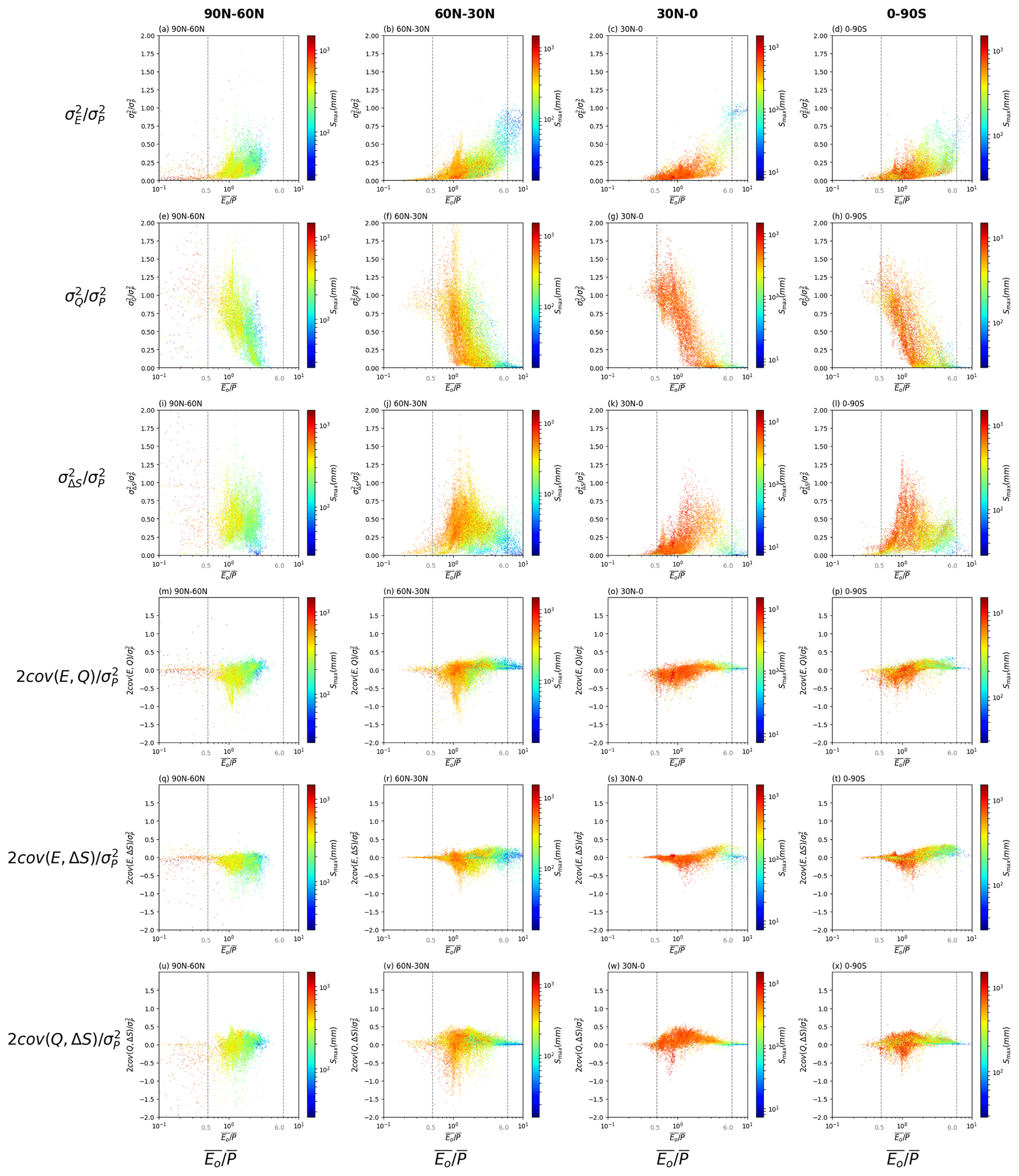
Figure 7Relation between water cycle variances and covariances (see Fig. 3b–g) as a fraction of the variance for P () and the aridity index () for grid cells over different latitude ranges (i.e. 90–60∘ N, 60–30∘ N, 30–0∘ N and 0–90∘ S). The colours relate to the water storage capacity Smax. Note that we have multiplied the covariances by two (see Eq. 2). The vertical grey dashed lines represent thresholds used to separate extremely dry () and wet () environments. Note the use of a logarithmic x axis and scale bar for Smax.
4.3.2 Relating inter-annual variability to mean air temperature
To understand the potential role of snow/ice in modifying the variance partitioning, we repeat the previous analysis (Fig. 7) but here we use the mean annual air temperature () to colour the grid cells to (crudely) indicate the presence of snow/ice (Fig. 8). The results are complex and not easy to simply understand. The most important difference revealed by this analysis is in the hydrologic partitioning between cold (first column) and hot (third column) conditions in wet environments (). In particular, when is high, is almost completely partitioned into in wet environments (e.g. , Fig. 8g). In contrast, when is low in a wet environment ( in first column of Fig. 8), there are substantial variations in the hydrologic partitioning. That result reinforces the complexity of variance partitioning in the presence of snow/ice.

Figure 8Relation between water cycle variances and covariances (see Fig. 3b–g) as a fraction of the variance for P () and the aridity index () for grid cells over different latitude ranges (i.e. 90–60∘ N, 60–30∘ N, 30–0∘ N and 0–90∘ S). The colours relate to the mean air temperature (). Note that we have multiplied the covariances by two (see Eq. 2). The vertical grey dashed lines represent thresholds used to separate extremely dry () and wet () environments.
4.4 Case studies
The previous results (Sect. 4.3) have demonstrated that the partitioning of is influenced by the water storage capacity (Smax) in extremely dry environments () and that the presence of snow/ice is important (as indicated by mean air temperature, ) in extremely wet environments (). In this section, we examine, in greater detail, several sites to gain deeper understanding of the partitioning of . For that purpose, we selected three sites based on extreme values for the three explanatory parameters, i.e. (Fig. S1a), Smax (Fig. S1b) and (Fig. S1c). The criteria to select three climate sites are as follows – Site 1: dry () and small Smax (), Site 2: dry () and relatively large Smax () and Site 3: wet () and hot ( ∘C). For each of the three classes, we use a representative grid cell (Fig. 9) to show the original time series (Fig. 10) and the partitioning of the variability (Fig. 11).
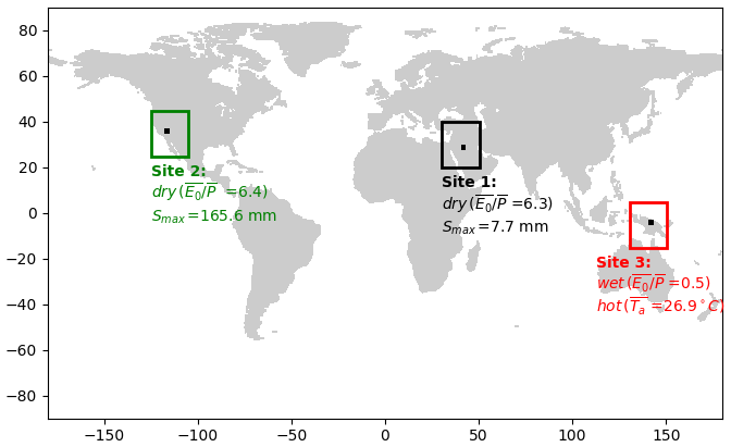
Figure 9Locations of three representative grid cells used as case study sites.
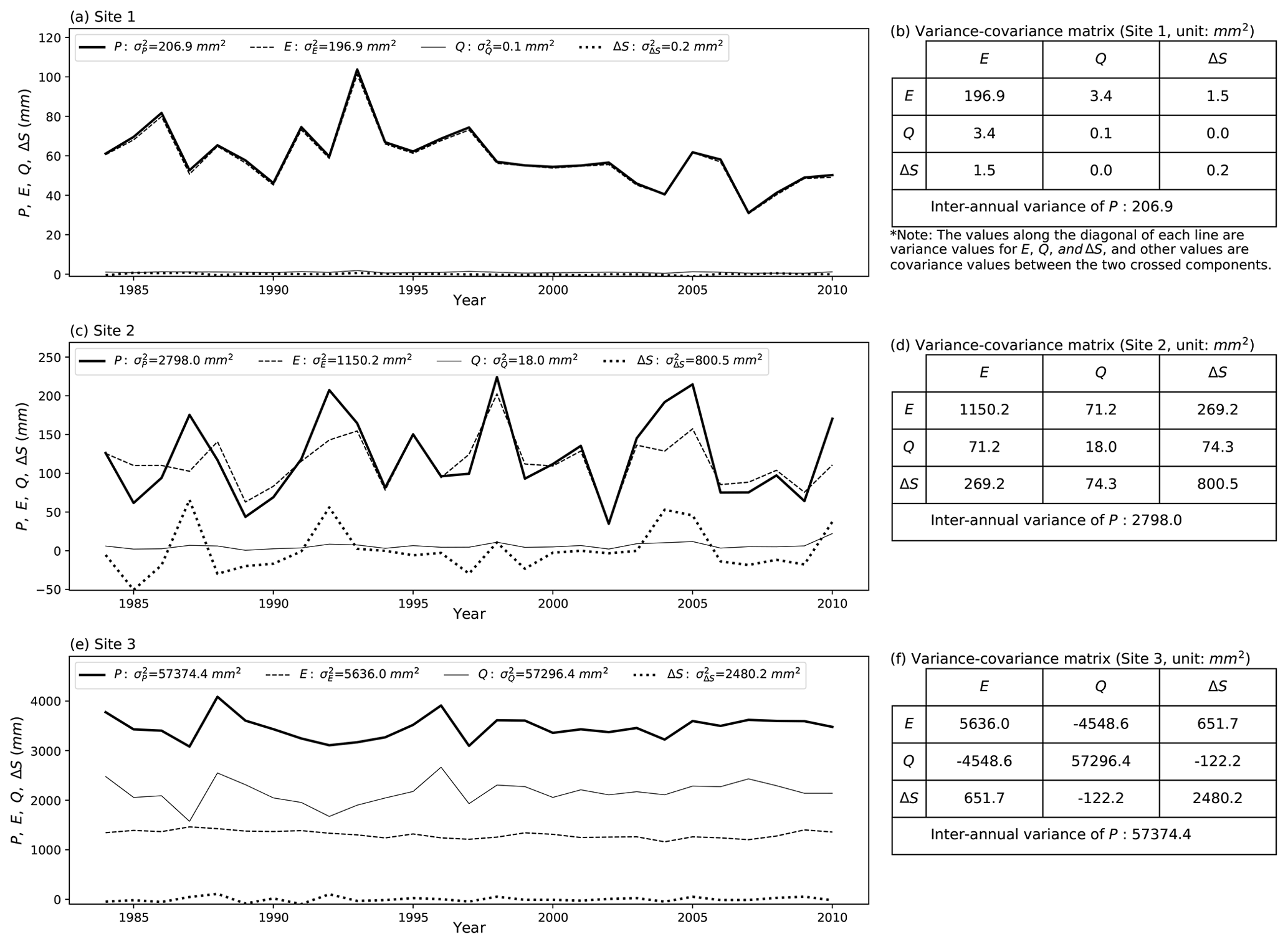
Figure 10Inter-annual time series (P, E, Q and ΔS) and the associated variance-covariance matrix (E, Q and ΔS) for case study Sites 1–3. Left column shows time series for (a) Site 1, (c) Site 2 and (e) Site 3, with right column, i.e. panels (b), (d) and (f), the associated variance–covariance matrix for three sites. Note that the covariance values in the tables should be multiplied by two to agree with the variance–covariance balance in Eq. (2).
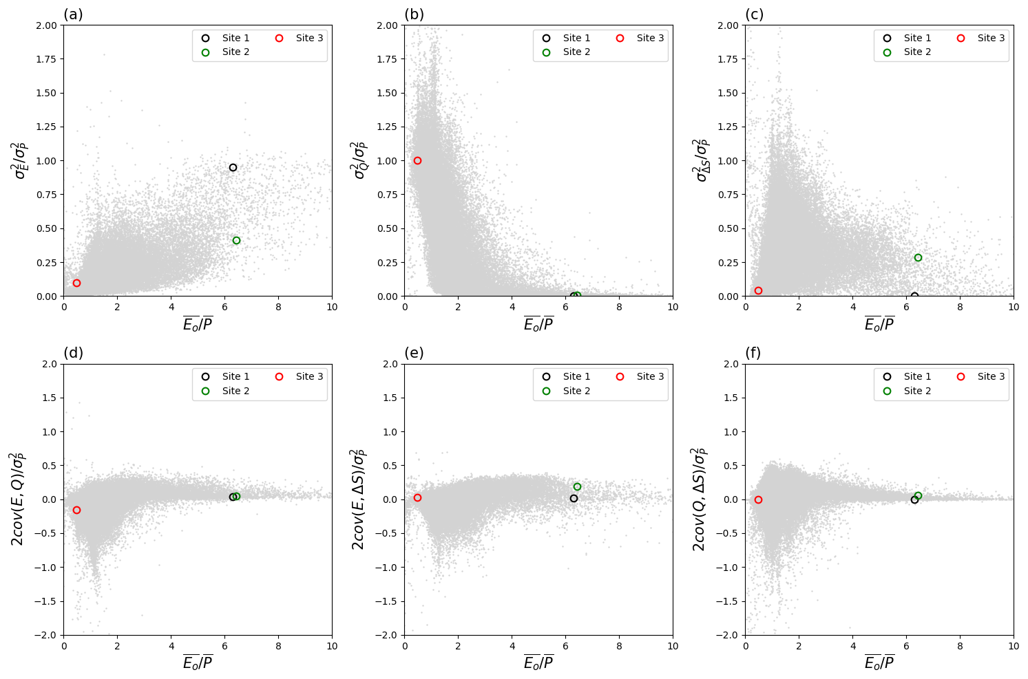
Figure 11Location of three case study sites in the water cycle variability space. The grey background dots are from Fig. 6.
We show the P, E, Q and ΔS time series along with the relevant variances and covariances in Fig. 10. Starting with the two dry sites, at the site with low storage capacity (Site 1), the time series shows that E closely follows P, leaving annual Q and ΔS close to zero (Fig. 10a). The variance of P ( mm2) is small and almost completely partitioned into the variance of E ( mm2), leaving very limited variance for Q, ΔS and all three covariance components (Fig. 10b). At the dry site with larger storage capacity (Site 2), E, Q and ΔS do not simply follow P (Fig. 10c). As a consequence, the variance of P ( mm2) is shared between E ( mm2), ΔS ( mm2) and their covariance component ( mm2, Fig. 10d). Switching now to the remaining wet and hot site (Site 3), we note that Q closely follows P, with ΔS close to zero and E showing little inter-annual variation (Fig. 10e). The variance of P ( mm2) is relatively large and almost completely partitioned into the variance of Q ( mm2), leaving very limited variance for E and ΔS and the three covariance components (Fig. 10f). We also examined numerous other sites with similar extreme conditions as the three case study sites and found the same basic patterns as reported above.
To put the data from the three case study sites into a broader variability context we position the site data onto a backdrop of Fig. 6. As noted previously, at Site 1, the ratio is very close to unity (Fig. 11a), and under this extreme condition, we have the following approximation:
In contrast, for Site 2 with the same aridity index but higher Smax, we have
Finally, at Site 3, we have
4.5 Synthesis
The above simple examples demonstrate that aridity , storage capacity Smax and, to a lesser extent, air temperature , all play some role in the partitioning of to the various components. Our synthesis of the results for the partitioning of is summarized in Fig. 12. In dry environments with low storage capacity () we have minimal runoff and expect that is more or less completely partitioned into (Fig. 12a). In those environments, (inter-annual) variations in storage play a limited role in setting the overall variability. However, in dry environments with larger storage capacity (), is only a small fraction of (Fig. 12a), leaving most of the overall variance in to be partitioned to and the covariance between E and ΔS (Fig. 12c and e). This emphasizes the hydrological importance of water storage capacity in buffering variations of the water cycle under dry conditions.
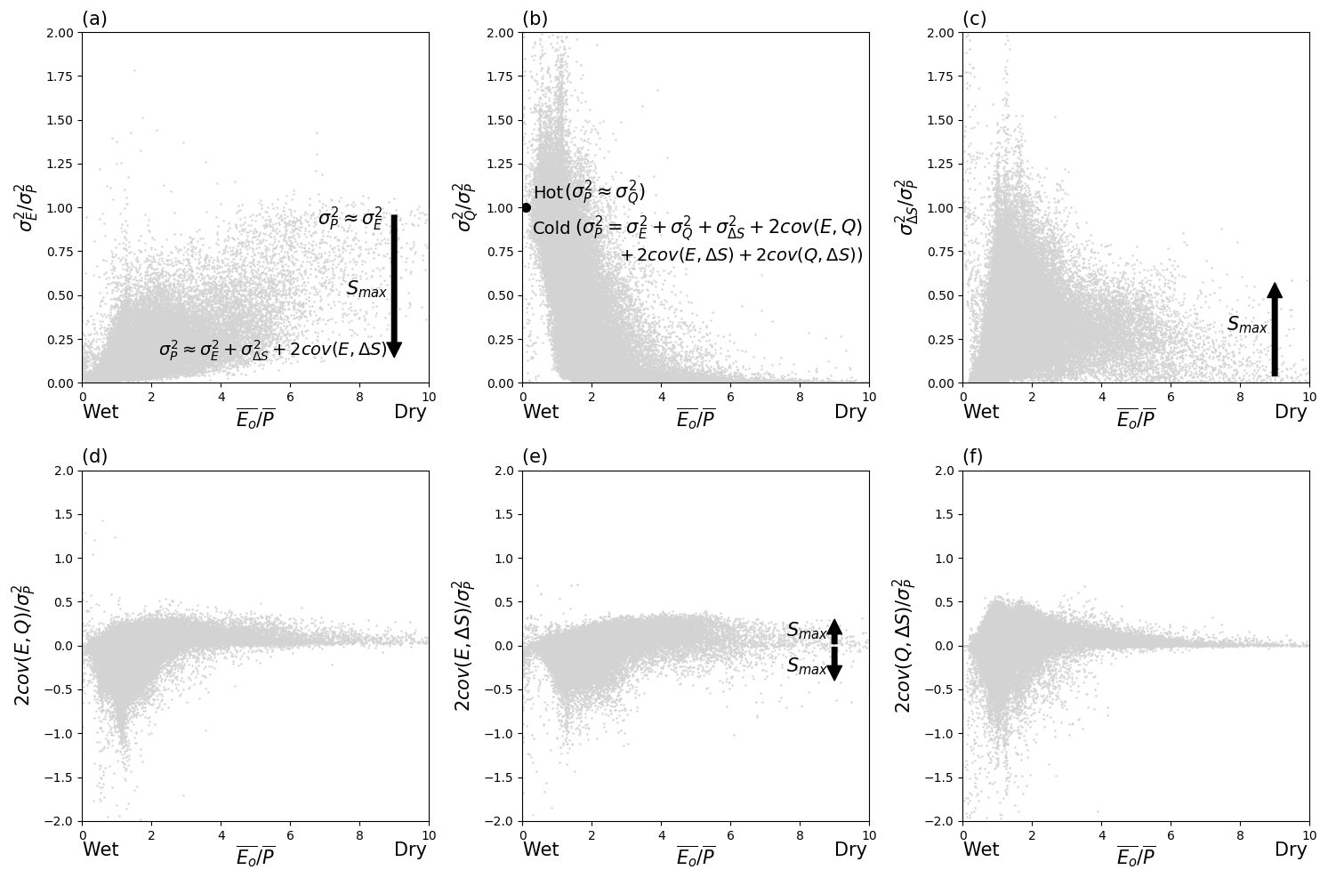
Figure 12Synthesis of factors controlling variance partitioning. The arrows denote trends with increasing Smax. The grey background dots are from Fig. 6.
Under extremely wet conditions, the largest difference in variance partitioning is not due to differences in storage capacity but is instead related to differences in mean air temperature. In wet and hot environments, we have maximum runoff and find that is more or less completely partitioned into (Fig. 12b) while the partitioning to and is small. However, in wet and cold environments, the variance partitioning shows great complexity, with being partitioned into all possible components. We suggest that this emphasizes the hydrological importance of thermal processes (melting/freezing) under extremely cold conditions.
However, the most complex patterns to interpret are those for semi-arid to semi-humid environments (i.e. ∼ 1.0). Despite a multitude of attempts over an extended period we were unable to develop a simple useful synthesis to summarize the partitioning of variability in those environments. We found that the three covariance terms all play important roles and we also found that simple environmental gradients (e.g. dry/wet, high/low storage capacity, hot/cold) could not easily explain the observed patterns. We anticipate that vegetation-related processes (e.g. phenology, rooting depth, gas exchange characteristics, disturbance) may prove to be important in explaining hydrologic variability in these biologically productive regions that support most of the human population. This result implies that a major scientific effort will be needed to develop a synthesis of the controlling factors for variability of the water cycle in these environments.
Importantly, hydrologists have long been interested in hydrologic variability, but without readily available databases it has been difficult to quantify water cycle variability. For example, we are not aware of maps showing global spatial patterns in variance for any terms of the water balance (except for P). In this study, we describe an initial investigation of the inter-annual variability of the terrestrial branch in the global water cycle that uses the recently released global monthly Climate Data Record (CDR) database for P, E, Q and ΔS. The CDR is one of the first dedicated hydrologic reanalysis databases and includes data for a 27-year period. Accordingly, we could only examine hydrologic variability over this relatively short period. Further, we expect future improvements and modifications as the hydrologic community seeks to further develop and refine these new reanalysis databases. With those caveats in mind, we started this analysis by first investigating the partitioning of P in the water cycle in terms of long-term mean and then extended that to the inter-annual variability using a theoretical variance balance equation (Eq. 2). Despite the initial nature of this investigation we have been able to establish some useful general principles.
The mean annual P is mostly partitioned into mean annual E and Q, as is well known, and the results using the CDR were generally consistent with the earlier Budyko framework (Fig. 2). Having established that, the first general finding is that the spatial pattern in the partitioning of inter-annual variability in the water cycle is not simply a reflection of the spatial pattern in the partitioning of the long-term mean. In particular, with the variance calculations, the annual anomalies are squared and hence the storage anomalies do not cancel out like they do when calculating the mean. With that in mind, we were surprised that the inter-annual variability of water storage change () is typically larger than the inter-annual variability of evapotranspiration () (cf. Fig. 3b and d). The consequence is that is more important than for understanding inter-annual variability of the global water cycle. A second important generalization is that unlike the variance components which are all positive, the three covariance components in the theory (Eq. 2) can be both positive and negative. We report results here showing both large positive and negative values for the three covariance terms (Fig. 3e, f, g). This was especially prevalent in biologically productive regions (, Fig. 3e, g). When examining the mean state, we are accustomed to think that P sets a limit to E, Q and ΔS, as per the mass balance (Eq. 1). But the same thinking does not extend to the variance balance since the covariance terms on the right-hand side of Eq. (2) can be both large and negative, leading to circumstances where the variability in the sinks (, , ) could actually exceed variability in the source (). These general principles of variance partitioning in the water cycle above may vary at different timescales (e.g. monthly, daily), and we expect more details of the variability partitioning across various temporal scales to be investigated in future studies.
Our initial attempt to develop deeper understanding of variance partitioning was based on a series of case studies located in extreme environments (wet/dry vs. hot/cold vs. high/low water storage capacity). The results offered some further insights about hydrologic variability. For example, under extremely dry (water-limited) environments, with limited storage capacity (Smax), we found that E follows P and follows , with and both approaching zero. However, as Smax increases, the partitioning of progressively shifts to a balance between , and cov(E,ΔS) (Figs. 10–12). This result explains the overestimation of σE∕σP by the empirical theory of Koster and Suarez (1999) which implicitly assumed no inter-annual change in storage. The Koster and Suarez empirical theory is perhaps better described as an upper limit that is based on minimal storage capacity, and that any increase in storage capacity would promote the partitioning of to , particularly under dry conditions (Figs. 10–12).
In extremely wet/hot environments (i.e. no snow/ice presence) we found to be mostly partitioned to (with both and approaching zero, Fig. 10). In contrast, in extremely wet/cold environments, the partitioning of was highly (spatially) variable, presumably because of spatial variability in the all-important thermal processes (freeze/melt).
The most complex results were found in mesic biologically productive environments (), where all three covariance terms (Eq. 2) were found to be relatively large and therefore they all played critical roles in the overall partitioning of variability (Fig. 6). As noted above, in many of these regions, the (absolute) magnitudes of the covariances were actually larger than the variances of the water balance components E, Q and ΔS (e.g. Fig. 3). That result demonstrates that deeper understanding of the process-level interactions that are embedded within each of the three covariance terms (e.g. the role of seasonal vegetation variation) will be needed to develop process-based understanding of variability in the water cycle in these biologically productive regions ().
The syntheses of the long-term mean water cycle originated in 1970s (Budyko, 1974), and it took several decades for those general principles to become widely adopted in the hydrologic community. The hydrologic data needed to understand hydrologic variability are only now becoming available. With those data we can begin to develop a process-based understanding of hydrologic variability that can be used for a variety of purposes; e.g. deeper understanding of hydro-climatic behaviour, hydrologic risk analysis, climate change assessments and hydrologic sensitivity studies are just a few applications that spring to mind. The initial results presented here show that a major intellectual effort will be needed to develop a general understanding of hydrologic variability.
The global terrestrial water budget used in this study can be accessed at http://stream.princeton.edu:8080/opendap/MEaSUREs/WC_MULTISOURCES_WB_050/ (Zhang et al., 2018). The NASA/GEWEX Surface Radiation Budget (SRB) is available at https://eosweb.larc.nasa.gov/project/srb/srb_table (last access: 10 August 2018; Stackhouse et al., 2011). The global land air temperature dataset from the Climatic Research Unit (CRU TS4.01 database) can be downloaded from http://data.ceda.ac.uk/badc/cru/data/cru_ts/cru_ts_4.01 (Harris et al., 2014). The FLUXNET data are available at https://fluxnet.fluxdata.org/ (last access: 8 March 2018). The LandFluxEval, MPI and E-RUN databases used for further validation are published by Mueller et al. (2013), Jung et al. (2010) and Gudmundsson and Seneviratne (2016b), respectively.
The supplement related to this article is available online at: https://doi.org/10.5194/hess-24-381-2020-supplement.
DY and MLR designed the study and are both responsible for the integrity of the manuscript. DY performed the calculations and analyses, and prepared the original manuscript, and MLR contributed to the interpretation, discussion and writing of the manuscript.
The authors declare that they have no conflict of interest.
We thank Anna Ukkola for help in accessing the FLUXNET database. We thank the reviewers (including René Orth and two anonymous reviewers) for helpful comments that improved the manuscript.
This research has been supported by the Australian Research Council (grant nos. CE11E0098 and CE170100023) and the National Natural Science Foundation of China (grant no. 51609122).
This paper was edited by Anke Hildebrandt and reviewed by Rene Orth and two anonymous referees.
Agarwal, D. A., Humphrey, M., Beekwilder, N. F., Jackson, K. R., Goode, M. M., and van Ingen, C.: A data-centered collaboration portal to support global carbon-flux analysis, Concurr. Comp-Pract. E., 22, 2323–2334, https://doi.org/10.1002/cpe.1600, 2010.
Baldocchi, D., Falge, E., Gu, L., Olson, R., Hollinger, D., Running, S., Anthoni, P., Bernhofer, C., Davis, K., Evans, R., Fuentes, J., Goldstein, A., Katul, G., Law, B., Lee, X., Malhi, Y., Meyers, T., Munger, W., Oechel, W., Paw U, K. T., Pilegaard, K., Schmid, H. P., Valentini, R., Verma, S., Vesala, T., Wilson, K., and Wofsy, S.: FLUXNET: A New Tool to Study the Temporal and Spatial Variability of Ecosystem-Scale Carbon Dioxide, Water Vapor, and Energy Flux Densities, B. Am. Meteorol. Soc., 82, 2415–2434, https://doi.org/10.1175/1520-0477(2001)082<2415:FANTTS>2.3.CO;2, 2001.
Balsamo, G., Albergel, C., Beljaars, A., Boussetta, S., Brun, E., Cloke, H., Dee, D., Dutra, E., Muñoz-Sabater, J., Pappenberger, F., de Rosnay, P., Stockdale, T., and Vitart, F.: ERA-Interim/Land: a global land surface reanalysis data set, Hydrol. Earth Syst. Sci., 19, 389–407, https://doi.org/10.5194/hess-19-389-2015, 2015.
Budyko, M. L.: Climate and Life. Academic Press, London, UK, 1974.
Choudhury, B. J.: Evaluation of an empirical equation for annual evaporation using field observations and results from a biophysical model, J. Hydrol., 216, 99–110, https://doi.org/10.1016/S0022-1694(98)00293-5, 1999.
Dee, D. P., Uppala, S. M., Simmons, A. J., Berrisford, P., Poli, P., Kobayashi, S., Andrae, U., Balmaseda, M. A., Balsamo, G., Bauer, P., Bechtold, P., Beljaars, A. C. M., van de Berg, L., Bidlot, J., Bormann, N., Delsol, C., Dragani, R., Fuentes, M., Geer, A. J., Haimberger, L., Healy, S. B., Hersbach, H., Hólm, E. V., Isaksen, L., Kållberg, P., Köhler, M., Matricardi, M., McNally, A. P., Monge-Sanz, B. M., Morcrette, J. J., Park, B. K., Peubey, C., de Rosnay, P., Tavolato, C., Thépaut, J. N., and Vitart, F.: The ERA-Interim reanalysis: configuration and performance of the data assimilation system, Q. J. Roy. Meteor. Soc., 137, 553–597, https://doi.org/10.1002/qj.828, 2011.
Fu, B. P.: On the Calculation of the Evaporation from Land Surface, Sci. Atmos. Sin., 5, 23–31, 1981.
Gudmundsson, L. and Seneviratne, S. I.: Observation-based gridded runoff estimates for Europe (E-RUN version 1.1), Earth Syst. Sci. Data, 8, 279–295, https://doi.org/10.5194/essd-8-279-2016, 2016a.
Gudmundsson, L. and Seneviratne, S. I.: E-RUN version 1.1: Observational gridded runoff estimates for Europe, link to data in NetCDF format (69 MB). PANGAEA, https://doi.org/10.1594/PANGAEA.861371, 2016b.
Gudmundsson, L., Greve, P., and Seneviratne, S. I.: The sensitivity of water availability to changes in the aridity index and other factors – A probabilistic analysis in the Budyko space, Geophys. Res. Lett., 43, 6985–6994, https://doi.org/10.1002/2016GL069763, 2016.
Harris, I., Jones, P. D., Osborn, T. J., and Lister, D. H.: Updated high-grids of monthly climatic observations – the CRU TS3. 10 Dataset, Int. J. Climatol., 34, 623–642, https://doi.org/10.1002/joc.3711, 2014 (data available at: http://data.ceda.ac.uk/badc/cru/data/cru_ts/cru_ts_4.01, last access: 8 March 2018).
Jackson, R. B., Canadell, J., Ehleringer, J. R., Mooney, H. A., Sala, O. E., and Schulze, E. D.: A Global Analysis of Root Distributions for Terrestrial Biomes, Oecologia, 108, 389–411, https://doi.org/10.1007/BF00333714, 1996.
Jung, M., Reichstein, M., Ciais, P., Seneviratne, S. I., Sheffield, J., Goulden, M. L., Bonan, G., Cescatti, A., Chen, J., de Jeu, R., Dolman, A. J., Eugster, W., Gerten, D., Gianelle, D., Gobron, N., Heinke, J., Kimball, J., Law, B. E., Montagnani, L., Mu, Q., Mueller, B., Oleson, K., Papale, D., Richardson, A. D., Roupsard, O., Running, S., Tomelleri, E., Viovy, N., Weber, U., Williams, C., Wood, E., Zaehle, S., and Zhang, K.: Recent decline in the global land evapotranspiration trend due to limited moisture supply, Nature, 467, 951–954, https://doi.org/10.1038/nature09396, 2010 (data available at: https://www.bgc-jena.mpg.de/geodb/projects/Data.php, last access: 7 March 2018).
Koster, R. D. and Suarez, M. J.: A Simple Framework for Examining the Interannual Variability of Land Surface Moisture Fluxes, J. Climate, 12, 1911–1917, https://doi.org/10.1175/1520-0442(1999)012<1911:ASFFET>2.0.CO;2, 1999.
McMahon, T. A., Peel, M. C., Pegram, G. G. S., and Smith, I. N.: A Simple Methodology for Estimating Mean and Variability of Annual Runoff and Reservoir Yield under Present and Future Climates, J. Hydrometeorol., 12, 135–146, https://doi.org/10.1175/2010jhm1288.1, 2011.
Milly, P. C. D.: Climate, soil water storage, and the average annual water balance, Water Resour. Res., 30, 2143–2156, https://doi.org/10.1029/94WR00586, 1994a.
Milly, P. C. D.: Climate, interseasonal storage of soil water, and the annual water balance, Adv. Water Resour., 17, 19–24, https://doi.org/10.1016/0309-1708(94)90020-5, 1994b.
Milly, P. C. D. and Dunne, K. A.: Macroscale water fluxes 1. Quantifying errors in the estimation of basin mean precipitation, Water Resour. Res., 38, 1205, https://doi.org/10.1029/2001WR000759, 2002.
Mueller, B., Hirschi, M., Jimenez, C., Ciais, P., Dirmeyer, P. A., Dolman, A. J., Fisher, J. B., Jung, M., Ludwig, F., Maignan, F., Miralles, D. G., McCabe, M. F., Reichstein, M., Sheffield, J., Wang, K., Wood, E. F., Zhang, Y., and Seneviratne, S. I.: Benchmark products for land evapotranspiration: LandFlux-EVAL multi-data set synthesis, Hydrol. Earth Syst. Sci., 17, 3707–3720, https://doi.org/10.5194/hess-17-3707-2013, 2013 (data available at: https://iac.ethz.ch/group/land-climate-dynamics/research/landflux-eval.html, last access: 7 March 2018).
Orth, R. and Destouni, G.: Drought reduces blue-water fluxes more strongly than green-water fluxes in Europe, Nat. Commun., 9, 3602, https://doi.org/10.1038/s41467-018-06013-7, 2018.
Padrón, R. S., Gudmundsson, L., Greve, P., and Seneviratne, S. I.: Large-Scale Controls of the Surface Water Balance Over Land: Insights From a Systematic Review and Meta-Analysis, Water Resour. Res., 53, 9659–9678, https://doi.org/10.1002/2017WR021215, 2017.
Reichle, R. H., Koster, R. D., De Lannoy, G. J. M., Forman, B. A., Liu, Q., Mahanama, S. P. P., and Touré, A.: Assessment and Enhancement of MERRA Land Surface Hydrology Estimates, J, Climate, 24, 6322–6338, https://doi.org/10.1175/JCLI-D-10-05033.1, 2011.
Rodell, M., Beaudoing, H. K., L'Ecuyer, T. S., Olson, W. S., Famiglietti, J. S., Houser, P. R., Adler, R., Bosilovich, M. G., Clayson, C. A., Chambers, D., Clark, E., Fetzer, E. J., Gao, X., Gu, G., Hilburn, K., Huffman, G. J., Lettenmaier, D. P., Liu, W. T., Robertson, F. R., Schlosser, C. A., Sheffield, J., and Wood, E. F.: The Observed State of the Water Cycle in the Early Twenty-First Century, J. Climate, 28, 8289–8318, https://doi.org/10.1175/JCLI-D-14-00555.1, 2015.
Roderick, M. L. and Farquhar, G. D.: A simple framework for relating variations in runoff to variations in climatic conditions and catchment properties, Water Resour. Res., 47, W00G07, https://doi.org/10.1029/2010WR009826, 2011.
Sankarasubramanian, A. and Vogel, R. M.: Annual hydroclimatology of the United States, Water Resour. Res., 38, 19-11–19-12, https://doi.org/10.1029/2001WR000619, 2002.
Scanlon, B. R., Zhang, Z., Save, H., Sun, A. Y., Müller Schmied, H., van Beek, L. P. H., Wiese, D. N., Wada, Y., Long, D., Reedy, R. C., Longuevergne, L., Döll, P., and Bierkens, M. F. P.: Global models underestimate large decadal declining and rising water storage trends relative to GRACE satellite data, P. Natl. Acad. Sci. USA, 115, E1080–E1089, https://doi.org/10.1073/pnas.1704665115, 2018.
Sposito, G.: Understanding the Budyko Equation, Water, 9, 236, https://doi.org/10.3390/w9040236, 2017.
Stackhouse, P. W., Gupta, S. K., Cox, S. J., Zhang, T., and Mikovitz, J. C.: NASA GEWEX Surface Radiation Budget, https://doi.org/10.17616/R37R42, 2011.
Ukkola, A. M., Haughton, N., De Kauwe, M. G., Abramowitz, G., and Pitman, A. J.: FluxnetLSM R package (v1.0): a community tool for processing FLUXNET data for use in land surface modelling, Geosci. Model Dev., 10, 3379–3390, https://doi.org/10.5194/gmd-10-3379-2017, 2017.
Wang, D. and Alimohammadi, N.: Responses of annual runoff, evaporation, and storage change to climate variability at the watershed scale, Water Resour. Res., 48, W05546, https://doi.org/10.1029/2011WR011444, 2012.
Wang-Erlandsson, L., Bastiaanssen, W. G. M., Gao, H., Jägermeyr, J., Senay, G. B., van Dijk, A. I. J. M., Guerschman, J. P., Keys, P. W., Gordon, L. J., and Savenije, H. H. G.: Global root zone storage capacity from satellite-based evaporation, Hydrol. Earth Syst. Sci., 20, 1459–1481, https://doi.org/10.5194/hess-20-1459-2016, 2016.
Yang, H., Yang, D., Lei, Z., and Sun, F.: New analytical derivation of the mean annual water-energy balance equation, Water Resour. Res., 44, W03410, https://doi.org/10.1029/2007WR006135, 2008.
Yang, Y., Donohue, R. J., and McVicar, T. R.: Global estimation of effective plant rooting depth: Implications for hydrological modeling, Water Resour. Res., 52, 8260–8276, https://doi.org/10.1002/2016WR019392, 2016.
Zeng, R. and Cai, X.: Assessing the temporal variance of evapotranspiration considering climate and catchment storage factors, Adv. Water Resour., 79, 51–60, https://doi.org/10.1016/j.advwatres.2015.02.008, 2015.
Zhang, Y., Pan, M., Sheffield, J., Siemann, A. L., Fisher, C. K., Liang, M., Beck, H. E., Wanders, N., MacCracken, R. F., Houser, P. R., Zhou, T., Lettenmaier, D. P., Pinker, R. T., Bytheway, J., Kummerow, C. D., and Wood, E. F.: A Climate Data Record (CDR) for the global terrestrial water budget: 1984–2010, Hydrol. Earth Syst. Sci., 22, 241–263, https://doi.org/10.5194/hess-22-241-2018, 2018 (data available at: http://stream.princeton.edu:8080/opendap/MEaSUREs/WC_MULTISOURCES_WB_050/, last access: 22 February 2018).
- Abstract
- Introduction
- Methods and data
- Mean and variability of water cycle components
- Relating the variability of water cycle components to aridity
- Discussion and conclusions
- Data availability
- Author contributions
- Competing interests
- Acknowledgements
- Financial support
- Review statement
- References
- Supplement