Rainfall estimation from a German-wide commercial microwave link network: optimized processing and validation for 1 year of data

Rainfall is one of the most important environmental variables. However, it is a challenge to measure it accurately over space and time. During the last decade, commercial microwave links (CMLs), operated by mobile network providers, have proven to be an additional source of rainfall information to complement traditional rainfall measurements. In this study, we present the processing and evaluation of a German-wide data set of CMLs. This data set was acquired from around 4000 CMLs distributed across Germany with a temporal resolution of 1 min. The analysis period of 1 year spans from September 2017 to August 2018. We compare and adjust existing processing schemes on this large CML data set. For the crucial step of detecting rain events in the raw attenuation time series, we are able to reduce the amount of misclassification. This was achieved by using a new approach to determine the threshold, which separates a rolling window standard deviation of the CMLs' signal into wet and dry periods. For the compensation for wet antenna attenuation, we compare a time-dependent model with a rain-rate-dependent model and show that the rain-rate-dependent model performs better for our data set. We use RADOLAN-RW, a gridded gauge-adjusted hourly radar product from the German Meteorological Service (DWD) as a precipitation reference, from which we derive the path-averaged rain rates along each CML path. Our data processing is able to handle CML data across different landscapes and seasons very well. For hourly, monthly, and seasonal rainfall sums, we found good agreement between CML-derived rainfall and the reference, except for the winter season due to non-liquid precipitation. We discuss performance measures for different subset criteria, and we show that CML-derived rainfall maps are comparable to the reference. This analysis shows that opportunistic sensing with CMLs yields rainfall information with good agreement with gauge-adjusted radar data during periods without non-liquid precipitation.

1 Introduction

Measuring precipitation accurately over space and time is challenging due to its high spatiotemporal variability. It is a crucial component of the water cycle, and knowledge of the spatiotemporal distribution of precipitation is an important quantity in many applications across meteorology, hydrology, agriculture, and climate research.

Typically, precipitation is measured by rain gauges, ground-based weather radars, or spaceborne microwave sensors. Rain gauges measure precipitation at the point scale. Errors can be caused, for example, by wind, solid precipitation, or evaporation losses (Sevruk, 2005). The main disadvantage of rain gauges is their lack of spatial representativeness.

Weather radars overcome this spatial constraint, but they are affected by other error sources. They do not directly measure rainfall but rather estimate it from related observed quantities, typically via the Z−R relation, which links the radar reflectivity “Z” to the rain rate “R”. This relation, however, depends on the rain drop size distribution (DSD), resulting in significant uncertainties. Dual-polarization weather radars reduce these uncertainties, but they still struggle with the DSD-dependence of the rain rate estimation (Berne and Krajewski, 2013). Additional error sources can stem from the measurement high above ground, from beam blockage, or from ground clutter effects.

Satellites can observe large parts of the Earth, but their spatial and temporal coverage also has limits. Geostationary satellites can provide a high temporal sampling rate of a specific part of the Earth; however, rain rate estimates show large uncertainties because they have to be derived from measurements of visible and infrared channels, which were not meant for this purpose. Satellites in low Earth orbits typically use dedicated sensors for rainfall estimation (microwave radiometers and radars), but their revisiting times are constrained by their orbits. Typical revisit times are in the order of hours to days. As a result, even merged multi-satellite products have a latency of several hours; for example, the Integrated Multi-satellite Retrievals (IMERG) early run of the Global Precipitation Measurement (GPM) mission has a latency of 6 h, while it is limited to a spatial resolution of 0.1^∘. The retrieval algorithms employed are highly sophisticated, and several calibration and correction stages are potential error sources (Maggioni et al., 2016).

Additional rainfall information, such as that derived from commercial microwave links (CMLs) maintained by cellular network providers, can be used to compare and complement existing rainfall data sets (Messer et al., 2006). In regions with sparse observation networks, they might even provide unique rainfall information.

The idea of deriving rainfall estimates from the opportunistic usage of attenuation data from CML networks emerged over a decade ago, independently in Israel (Messer et al., 2006) and the Netherlands (Leijnse et al., 2007). The main research foci in the first decade of dedicated CML research were the development of processing schemes for the rainfall retrieval and the reconstruction of rainfall fields. The first challenge for rainfall estimation from CML data is to distinguish between fluctuations of the raw attenuation data during rainy and dry periods. This was addressed by different approaches which either compared neighboring CMLs using the spatial correlation of rainfall (Overeem et al., 2016a) or focused on analyzing the time series of individual CMLs (Chwala et al., 2012; Polz et al., 2019; Schleiss and Berne, 2010; Wang et al., 2012). Another challenge is to estimate and correct the effect of wet antenna attenuation. This effect stems from the attenuation caused by water droplets on the covers of CML antennas, which leads to rainfall overestimation (Fencl et al., 2019; Leijnse et al., 2008; Schleiss et al., 2013).

As many hydrological applications require spatial rainfall information, several approaches have been developed for the generation of rainfall maps from the path-integrated CML measurements. Kriging was successfully applied to produce countrywide rainfall maps for the Netherlands (Overeem et al., 2016b), representing CML rainfall estimates as synthetic point observations at the center of each CML's path. More sophisticated methods can account for the path-integrated nature of the CML observations, using an iterative inverse distance weighting approach (Goldshtein et al., 2009), stochastic reconstruction (Haese et al., 2017), or tomographic algorithms (D'Amico et al., 2016; Zinevich et al., 2010).

CML-derived rainfall products have also been used to derive combined rainfall products from various sources (Fencl et al., 2017; Liberman et al., 2014; Trömel et al., 2014). In parallel, the first hydrological applications were tested. CML-derived rainfall was used as model input for hydrologic modeling studies for urban drainage modeling with synthetic (Fencl et al., 2013) and real-world data (Stransky et al., 2018) or on runoff modeling in natural catchments (Brauer et al., 2016; Smiatek et al., 2017).

With the exception of the research carried out in the Netherlands, where more than 2 years of data from a countrywide CML network were analyzed (Overeem et al., 2016b), CML processing methods have only been tested on small data sets. We advance the state of the art by performing an analysis of rainfall estimates derived from a German-wide network of close to 4000 CMLs. In this study, one CML is counted as the link along one path, typically with two sub-links, for communication in both directions. The temporal resolution of the data set is 1 min, and the analysis period is 1 year (from September 2017 to August 2018). The network covers various landscapes from the North German Plain to the Alps in the south, which feature individual precipitation regimes.

The objectives of this study are (1) to compare and adjust selected existing CML data processing schemes for the classification of wet and dry periods and for the compensation of wet antenna attenuation and (2) to validate the derived rain rates with an established rainfall product, namely RADOLAN-RW, both on the countrywide scale of Germany.

2 Data

2.1 Reference data set

The Radar-Online-Aneichung data set (RADOLAN-RW) from the German Weather Service (DWD) is a radar-based and gauge-adjusted precipitation data set. We use data from the archived real-time RADOLAN-RW product as a reference data set throughout this work (DWD, 2019). It is a compiled radar composite from 17 dual-polarization weather radars operated by DWD and adjusted by more than 1000 rain gauges in Germany and 200 rain gauges from surrounding countries. However, RADOLAN-RW does not use dual-pol information. It is based on the reflectivity observations in horizontal polarization from each radar site, which are available in real time every 5 min. These data are then used to compile a national composite of reflectivities, from which rain rates are derived. For the hourly rainfall information of the RADOLAN-RW product, the national composite of 5 min radar rain rates is then aggregated and adjusted with the hourly rain gauge observations. A weighted mixture of additive and multiplicative corrections is applied. The rain gauges used for the adjustment have a spatial density of approximately one gauge per 300 km².

The gridded RADOLAN-RW data set has a spatial resolution of 1 km, covering Germany with 900 × 900 grid cells. The temporal resolution is 1 h, and the rainfall values are given with a quantization of 0.1 mm. RADOLAN-RW is available with a lag time of around 15 min. Detailed information on the RADOLAN processing and products is available from DWD (Bartels et al., 2004; Winterrath et al., 2012).

Kneis and Heistermann (2009) and Meissner et al. (2012) compared RADOLAN-RW products to gauge-based data sets for small catchments and found differences in daily, area-averaged precipitation sums of up to 50 %, especially for the winter season. Nevertheless, no data set with comparable temporal and spatial resolution, as well as extensive quality control, is available.

In order to compare the path-integrated rainfall estimates from CMLs and the gridded RADOLAN-RW product, RADOLAN-RW rain rates are resampled along the individual CML paths. For each CML, the weighted average of all intersecting RADOLAN-RW grid cells is calculated, with the weights being the lengths of the intersecting CML path in each cell. As a result, one time series of the hourly rain rate is generated from RADOLAN-RW for each CML. The temporal availability of this reference is 100 %; however, we excluded the CML and RADOLAN-RW pairs for which CML data were unavailable from the evaluation. We chose the RADOLAN-RW product because it provides both a high temporal and spatial resolution throughout Germany. This resolution is the basis for the evaluation of the path-averaged rain rates derived from CMLs. The rain gauge adjustment, while not perfect, assures that the RADOLAN-RW rainfall estimates have an increased accuracy compared with a radar-only data set.

2.2 Commercial microwave link data

We present data from 3904 CMLs operated by Ericsson in Germany. Their distribution throughout Germany is shown in Fig. 1. The CMLs are distributed countrywide and cover all landscapes, ranging from the North German Plain to the Alps in the south. The uneven distribution, with large gaps in the northeast can be explained by the fact that we only access one subset of all CMLs installed, the Ericsson MINI-LINK Traffic Node systems operated for one cell phone provider.

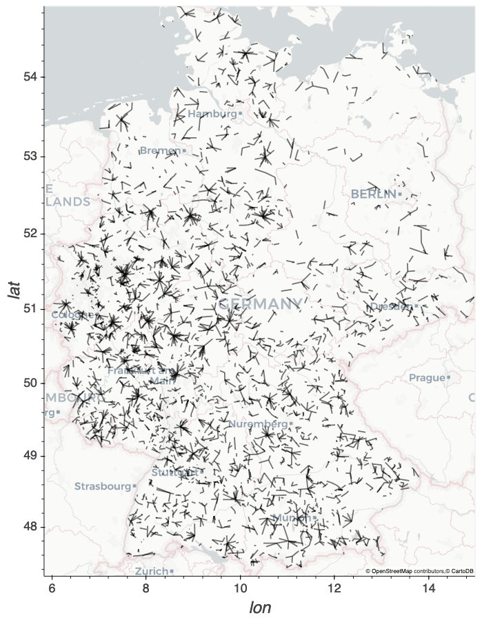
Figure 1 Map of the distribution of 3904 CMLs throughout Germany. © OpenStreetMap contributors 2019. Distributed under a Creative Commons BY-SA license.

CML data are retrieved with a real-time data acquisition system that we operate in cooperation with Ericsson (Chwala et al., 2016). Every minute, the current transmitted signal level (TSL) and received signal level (RSL) are requested from more than 4000 CMLs for both ends of each CML. The data are then immediately sent to and stored at our server. For the complete processing chain presented in this work, we used this 1 min instantaneous TSL and RSL data for the period from September 2017 to August 2018 for 3904 CMLs to derive rain rates with a temporal resolution of 1 min. For comparison with the reference data, the 1 min data are then aggregated. Due to missing, unclear, or corrupted metadata, we could not use all CML data. Furthermore, we only used data from one sub-link per CML. There was no specific criterion for selecting the sub-link. We simply used the pair of TSL and RSL that came first in our listing.

The available power resolution is 1 dB for TSL and 0.3 dB (with occasional jumps of 0.4 dB) for RSL. The TSL is constant for 25 % of the CMLs. An automatic transmit power control (ATPC), which is able to increase TSL by several decibels to prevent blackouts due to heavy attenuation, is active at 75 % of the CMLs. While the length of the CMLs ranges from a few hundred meters to almost 30 km, most CMLs have a length of 5 to 10 km. They are operated at frequencies ranging from 10 to 40 GHz, depending on their length. Figure 2 shows the distributions of path lengths and frequencies. For shorter CMLs, higher frequencies are used.

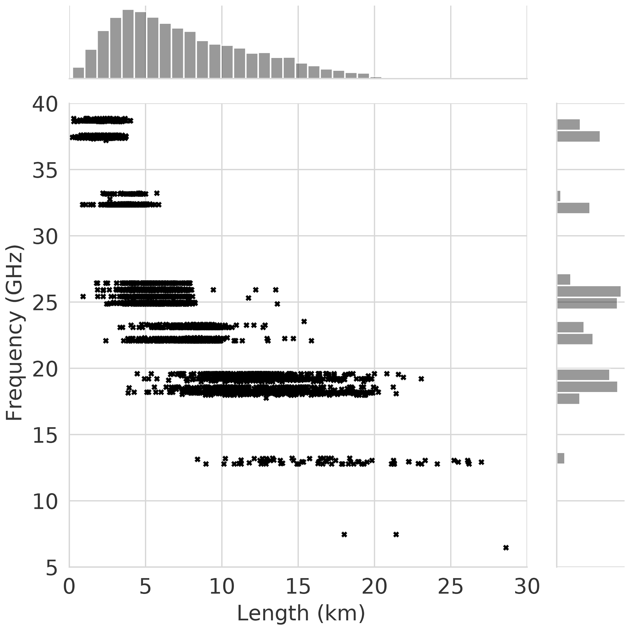
Figure 2 Scatterplot of the length against the microwave frequency of 3904 CMLs, including the distribution of length and frequency.

To derive rainfall from CMLs, we used the difference between TSL and RSL (the transmitted minus received signal level, TRSL). An example of a TRSL time series is shown in Fig. 3a. To compare the rain rate derived from CMLs with the reference rain rate, we resampled the temporal resolution from 1 min to 1 h after the processing.

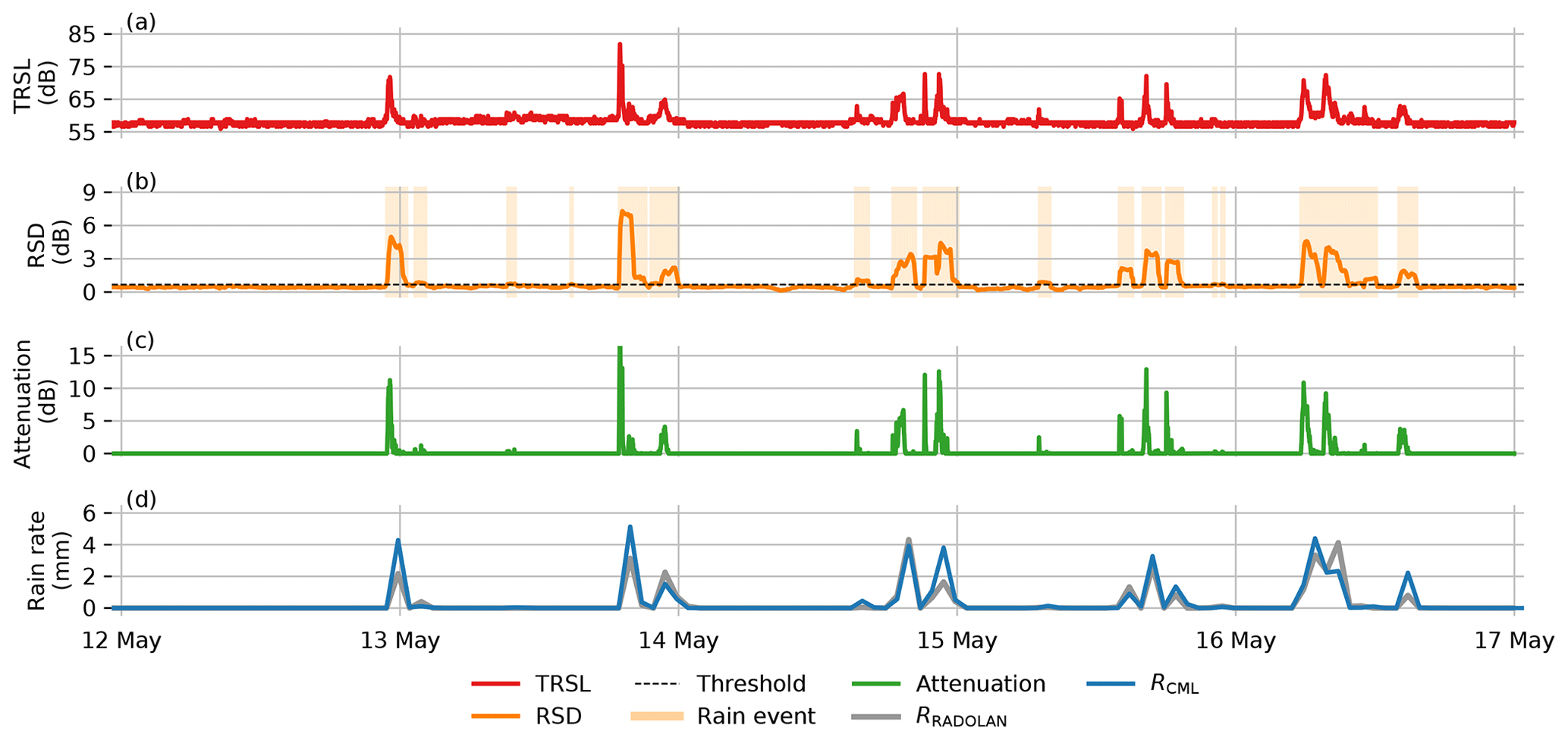
Figure 3 Processing steps from the TRSL to rain rate. (a) The TRSL is the difference between TSL and RSL (TSL minus RSL) – the raw transmitted and received signal level of a CML. (b) The RSD (rolling standard deviation) of the TRSL with an exemplary threshold shows the resulting wet and dry periods. (c) The attenuation is the difference between the baseline and the TRSL during wet periods. (d) The derived rain rate is resampled to an hourly scale in order to compare it to the reference (RADOLAN-RW).

In our CML data set, 2.2 % of the data are missing time steps due to outages of the data acquisition systems. Additionally 1.2 % of the raw data show missing values (Nan) and 0.1 % show default fill values (e.g., −99.9 or 255.0) of the CML hardware, which we excluded from the analysis. In order to increase the data availability, we linearly interpolated gaps in the raw TRSL time series that were up to 5 min long. This increased the data availability by 0.5 %. These gaps could have been the result of missing time steps and missing values, but we also found cases where we suspect very high rainfall to be the reason for short blackouts of a CML.

The size of the complete CML data set is approximately 100 GB (in memory). The data set is continuously extended by the operational data acquisition, also allowing for the possibility of near-real-time rainfall estimation.

3 Methods

3.1 Performance measures

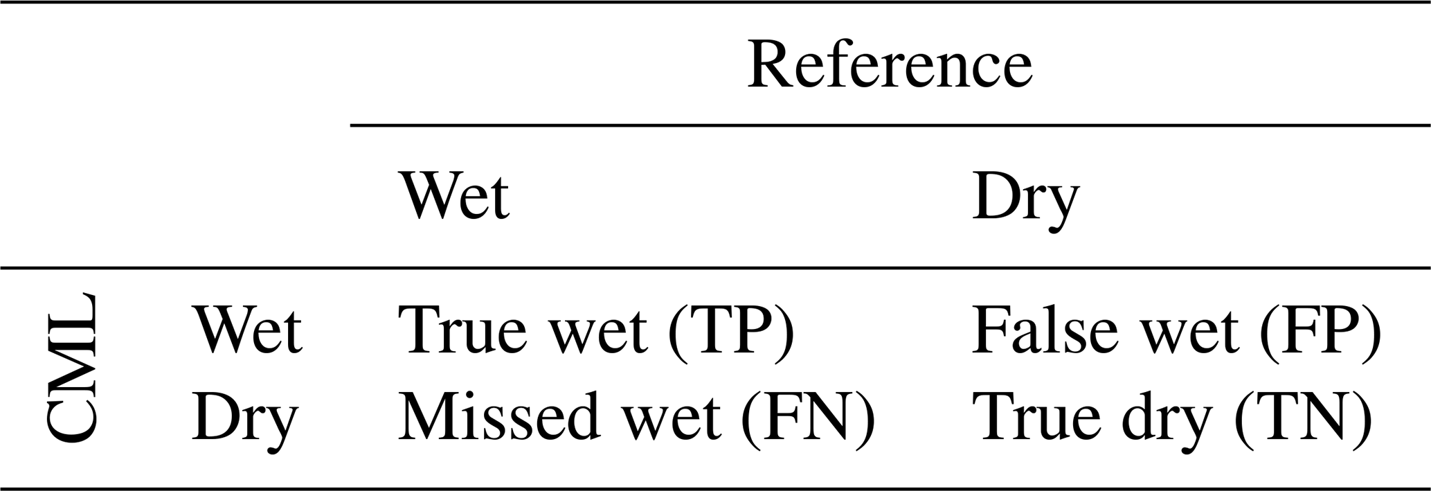
To evaluate the performance of the CML-derived rain rates against the reference data set, we used several measures which we calculated on an hourly basis. We defined a confusion matrix according to Table 1 where “Wet” and “Dry” refer to hours with and without rain, respectively.

Table 1 Confusion matrix of CML and reference data.

The Matthews correlation coefficient (MCC) summarizes the four values of the confusion matrix in a single measure (Eq. 1) and is typically used as measure of binary classification in machine learning. This measure accounts for the skewed ratio of wet and dry events. It is only high if the classifier performs well on both classes.

$$\begin{array}{}\text{(1)}& \mathrm{MCC}={\displaystyle \frac{\mathrm{TP}\times \mathrm{TN}-\mathrm{FP}\times \mathrm{FN}}{\sqrt{(\mathrm{TP}+\mathrm{FP})(\mathrm{TP}+\mathrm{FN})(\mathrm{TN}+\mathrm{FP})(\mathrm{TN}+\mathrm{FN})}}}\end{array}$$

The mean detection error (MDE; Eq. 2) is introduced as a further binary measure, focusing on the misclassification of rain events.

$$\begin{array}{}\text{(2)}& \mathrm{MDE}={\displaystyle \frac{\frac{\mathrm{FN}}{n\left(\mathrm{wet}\right)}+\frac{\mathrm{FP}}{n\left(\mathrm{dry}\right)}}{\mathrm{2}}}\end{array}$$

It is calculated as the average of missed wet and false wet rates of the confusion matrix (Table 1).

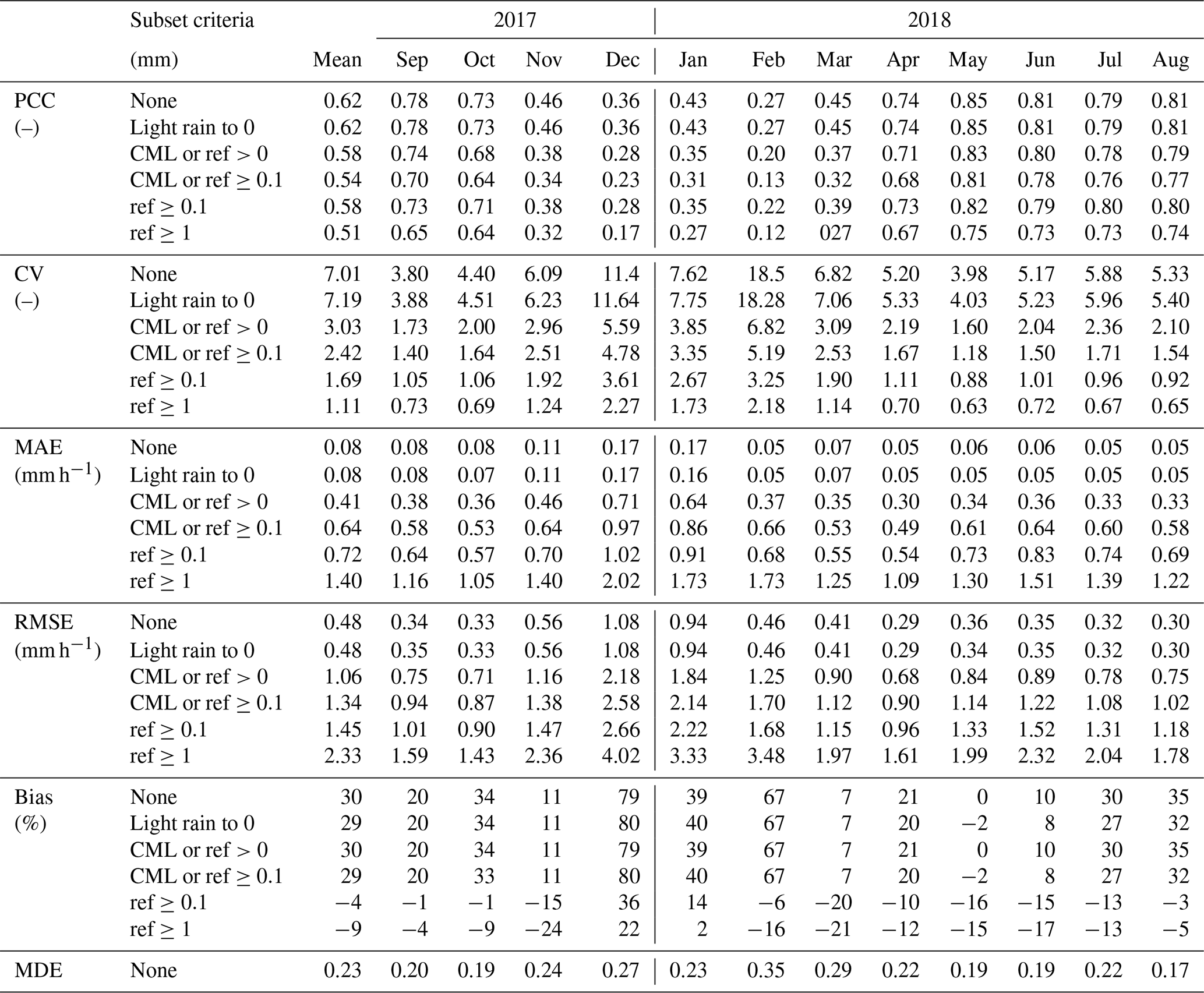
Table 2 Monthly performance measures between path-averaged, hourly CML-derived rainfall (R_CML) and RADOLAN-RW as a reference (R_reference, shortened here to “ref”) for subset criteria and thresholds.

The linear correlation between CML-derived rainfall and the reference is expressed by the Pearson correlation coefficient (PCC). The coefficient of variation (CV) in Eq. (3) gives the distribution of CML rainfall around the reference expressed by the ratio of the residual standard deviation to the mean reference rainfall:

$$\begin{array}{}\text{(3)}& \mathrm{CV}={\displaystyle \frac{\mathrm{SD}\sum \left(R_{\mathrm{CML}}-R_{\mathrm{reference}}\right)}{\stackrel{\mathrm{‾}}{R_{\mathrm{reference}}}}},\end{array}$$

where R_CML and R_reference are hourly rain rates of the respective data set. Furthermore, we computed the mean absolute error (MAE) and the root-mean-squared error (RMSE) to measure the accuracy of the CML rainfall estimates. The relative bias is given as follows:

$$\begin{array}{}\text{(4)}& \mathrm{bias}={\displaystyle \frac{\stackrel{\mathrm{‾}}{\left(R_{\mathrm{CML}}-R_{\mathrm{reference}}\right)}}{\stackrel{\mathrm{‾}}{R_{\mathrm{reference}}}}}\end{array}$$

Often, in studies comparing CML-derived rainfall and radar data, a threshold is used as a lower boundary for rainfall. The performance measures, summarized in Table 2, were calculated with different subset criteria or thresholds. This gives insight into how CML-derived rainfall compares to the reference for different rain rates and on how the large number of data points without rain influences the performance measures. Another reason for listing the performance measures with several thresholds is the increased comparability with other studies on CML rainfall estimation, which do not uniformly use the same threshold (see, e.g., Table A1 in de Vos et al., 2019). Therefore, we defined a selection of subset criteria and thresholds and show performance measures for data without any thresholds (“None”), for the data set with R_CML and R_reference<0.1 mm h⁻¹ set to 0 mm h⁻¹, for two thresholds where at least R_CML or R_reference must be >0 and ≥0.1 mm h⁻¹, and two thresholds where R_reference must be ≥0.1 and ≥1 mm.

3.2 From raw signal to rain rate

As CMLs are an opportunistic sensing system rather than part of a dedicated measurement system, data processing has to be done with care. Most of the CML research groups have developed their own methods that are tailored to their needs and data sets. Overviews of these methods are summarized by Chwala and Kunstmann (2019), Messer and Sendik (2015), and Uijlenhoet et al. (2018).

The size of our data set is a challenge in itself. As TRSL can be attenuated by rain or other sources, as described in Sect. 3.2.1, and only raw TSL and RSL data are provided, the large size of the data set is advantageous but also challenging. Developing and evaluating methods was significantly sped up by the use of an automated processing workflow, which we implemented as a parallelized workflow on a high-performance computing (HPC) system using the “xarray” and “Dask” Python packages for data processing and visual exploration. The major challenges that arose from the processing of raw TRSL data into rain rates and the selected methods from the literature are described in the following sections. We used parameters in this processing that are either based on the literature, modified from the literature, or which we developed in this study. An overview of all of the parameters used is given in Appendix A1.

3.2.1 Erratic behavior

Rainfall is not the only source of microwave radio attenuation along a CML path. Additional attenuation can be caused by atmospheric constituents like water vapor or oxygen and also by refraction, reflection, or multipath propagation of the beam (Upton et al., 2005). In particular, refraction, reflection, and multipath propagation can lead to strong attenuation that is of the same magnitude as that from rain. CMLs that exhibit such behavior have to be omitted due to their noisiness.

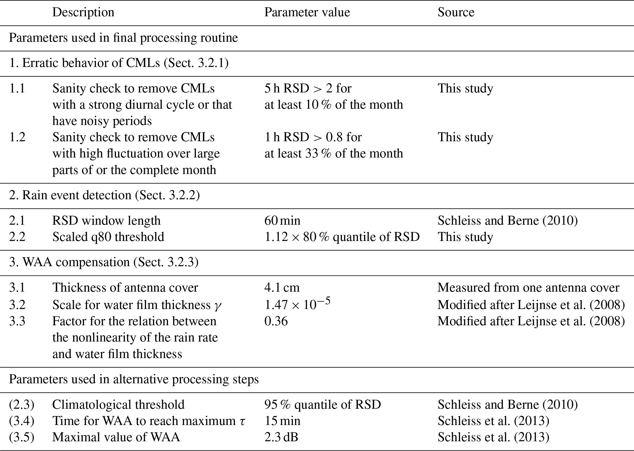
We excluded erratic CML data that were extremely noisy or that showed drifts and jumps from our analysis on a monthly basis. To deal with these erratic data, we applied the following sanity checks: we excluded individual CMLs if (1) the 5 h moving window standard deviation exceeded the threshold of 2.0 for more then 10 % of a month, which is typically the case for CMLs with either a strong diurnal cycle or very noisy periods during a month, or if (2) a 1 h moving window standard deviation exceeded the threshold of 0.8 more than 33 % of the time in a month. This filter was based on the approach for detecting rain events in TRSL time series from Schleiss and Berne (2010), which we also use later on in our processing. For the filter, a fairly high threshold was used, which should only be exceeded for fluctuations stemming from real rain events. The reasoning for our filter is that if the threshold is exceeded too often, here 33 % of the time per month, the CML data show an unreasonably high amount of strong fluctuation. In total, the two sanity checks removed 1.1 % of the data from our CML data set. In combination with the missing values that remain after interpolating data gaps of a maximum of 5 min in the TRSL time series, 4.2 % of our data set is unavailable or not used for processing.

Jumps in data are mainly caused by single default values in the TSL, which are described in Sect. 2.2. When we removed these default values, we are able to remove the jumps. TRSL can drift and fluctuate on a daily and yearly scale (Chwala and Kunstmann, 2019). We could neglect the influence of these drifts in our analysis, because we dynamically derived a baseline for each rain event (as explained in Sect. 3.2.2). We also excluded CMLs with a constant TRSL over a whole month.

3.2.2 Rain event detection and baseline estimation

The TRSL during dry periods can fluctuate over time due to ambient conditions, as mentioned in the previous section. Rainfall produces additional attenuation on top of the dry fluctuation. In order to calculate the attenuation from rainfall, a baseline level of TRSL during each rain event has to be determined. We derived the baseline from the precedent dry period. During the rain event, this baseline was held constant as no additional information on the evolution of the baseline level was available. The crucial step for deriving the baseline is to separate the TRSL time series into wet and dry periods, because then only the correct reference level before a rain event is used. By subtracting the baseline from TRSL, we derived the attenuation caused by rainfall, which is shown in Fig. 3c.

The separation of wet and dry periods is essential, because the errors made in this step will impact the performance of the rainfall estimation: missing rain events will result in rainfall underestimation, and the false detection of rain events will lead to overestimation. The task of detecting rain events in the TRSL time series is simple for strong rain events, but it is challenging when the attenuation from rain approaches the same order of magnitude as the fluctuation of TRSL data during dry conditions.

There are two essential concepts to detect rain events: one compares the TRSL of a certain CML to neighboring CMLs (Overeem et al., 2016a), and the other investigates the time series of each CML separately (Chwala et al., 2012; Schleiss and Berne, 2010; Wang et al., 2012). We chose the latter and used a rolling standard deviation (RSD) with a centered moving window of 60 min as a measure for the fluctuation of TRSL, as proposed by Schleiss and Berne (2010).

It is assumed that RSD is high during wet periods and low during dry periods. Therefore, an adequate threshold can be defined that differentiates the RSD time series into wet and dry periods. An example of an RSD time series and a threshold is shown in Fig. 3b, and all data points with RSD values above the threshold are considered to be wet.

Schleiss and Berne (2010) proposed the use of a RSD threshold derived from rainfall climatology (e.g., from nearby rain gauges). For our data set, we assumed that it was raining for 5 % of all minutes in Germany, as proposed by Schleiss and Berne (2010) for their CMLs in France. Therefore, we used the 95 % quantile of the RSD as a threshold, assuming that the 5 % of data with the highest fluctuation of the TRSL time series refer to the 5 % of rainy periods. We refer to this threshold as the climatological threshold. We compared it to two new definitions of thresholds. We are aware that this threshold does not reflect the real climatology at each CML location; nevertheless, this method is a rather robust and a simple approach that provides a first rain event detection.

For the first new definition, we derived the optimal threshold for each CML based on our reference data for the month of May 2018. We used the same approach as for the climatological threshold, but we tested a range of possible thresholds for each CML and calculated the binary measure MCC for each threshold. For each CML, we picked the threshold that produced the highest MCC in May 2018 and used it over the whole analysis period.

The second new definition to derive a threshold is based on the quantiles of the RSD, similarly to the climatological threshold described above. However, we propose not focusing on the fraction of rainy periods to find the optimal threshold, as a rainfall climatology is likely not valid for individual years and is not easily transferable to different locations. We took the 80th quantile of the RSD of each CML, which can be interpreted as a measure of the strength of the TRSL fluctuation during dry periods, and multiplied it by a constant factor to derive the individual threshold. The 80th quantile can be assumed to be more robust than the climatological threshold with respect to misclassification, because this quantile represents the general tendency of each TRSL time series to fluctuate rather than the percentage of time in which it is raining. We chose the 80th quantile as it is very unlikely that it is raining more than 20 % of the time in a month in Germany.

To find the right factor, we selected the month of May in 2018 and fitted a linear regression between the optimal threshold for each CML and the 80th quantile. The optimal threshold was derived beforehand using a MCC optimization from the reference. We then used this factor for all other months in our analysis. We found it to be similar for all months in the analysis period.

3.2.3 Wet antenna attenuation

Wet antenna attenuation (WAA) is the attenuation caused by water on the cover of a CML antenna. With this additional attenuation, the derived rain rate overestimates the true rain rate (Schleiss et al., 2013; Zinevich et al., 2010). The estimation of WAA is complex, as it is influenced by partially unknown factors, such as the material of the antenna cover. A study by van Leth et al. (2018) found differences in the WAA magnitude and temporal dynamics due to different sizes and shapes of the water droplets on hydrophobic and normal antenna cover materials. Another unknown factor regarding the determination of WAA is whether both, one, or none of the antennas of a CML are wetted during a rain event. We selected and compared two parametric WAA correction schemes that do not rely on the use of auxiliary data, such as nearby rain gauges.

Schleiss et al. (2013) measured the magnitude and dynamics of WAA with one CML in Switzerland and derived a time-dependent WAA model. In this model, WAA increases at the beginning of a rain event to a defined maximum over a defined amount of time. From the end of the rain event on, WAA decreases again, as the wetted antenna dries off. We ran this scheme with the proposed 2.3 dB of maximal WAA for both antennas together. This value is similar to the WAA correction value of 2.15 dB, which Overeem et al. (2016b) derived over a 12 d period in their data set. For τ, which determines the increase rate with time, we chose 15 min. The decrease in WAA after a rain event is not explicitly modeled, because this WAA scheme is only applied for time steps that are considered wet from the previous processing step of detecting rain events.

Leijnse et al. (2008) proposed a physical approach where the WAA depends on the microwave frequency, the antenna cover properties (thickness and refractive index), and the rain rate. A homogeneous water film is assumed to exist on the antenna, with a thickness that has a power law dependence on the rain rate. Higher rain rates cause a thicker water film and, hence, higher WAA. A factor γ scales the thickness of the water film on the cover, and a factor δ determines the nonlinearity of the relation between the rain rate and water film thickness. We adjusted the thickness of the antenna cover to 4.1 mm, which we measured from one antenna provided by Ericsson. We are aware of the fact that antenna covers have different thicknesses; however, as we do not have this information for the actual antennas that are used by the CMLs producing our data, we use this value as it is the best estimate available. We further adjusted γ to $\mathrm{1.47}\times {\mathrm{10}}^{-\mathrm{5}}$ and δ to 0.36 in such a way that the increase in WAA with rain rates is less steep for lower rain rates compared with the originally proposed parameters. The original set of parameters suppressed small rain events too much because the WAA compensation attributed all attenuation in the TRSL to WAA. For strong rain events (>10 mm h⁻¹), the maximum WAA that is reached with our set of parameters is in the same range as the 2.3 dB used as a maximum in the approach of Schleiss et al. (2013).

We want to note that several recent methods quantifying the WAA were developed using auxiliary information, such as rain gauge data. This is the reason we did not consider these approaches, as we wanted our CML data processing to be as applicable to new regions as possible. However, the transferability of WAA estimation methods remains an open scientific question. Fencl et al. (2019) quantified the influence of WAA for eight very short (length <500 m) CMLs using cumulative distribution functions from attenuation and rain gauge data. Their approach is not applicable to new CMLs, as it requires calibration for each individual CML based on the local rainfall and attenuation statistics. Ostrometzky et al. (2018) used a rain gauge to estimate the WAA of an E-band CML. They calculated both the (dry, constant during rain events) baseline and the theoretical attenuation using rain gauge data and attributed the residual attenuation to WAA. Moroder et al. (2020) developed a model involving the dynamic antenna parameters of reflectivity, efficiency, and directivity based on a full-wave simulation and applied it to a dedicated experimental setup with CML antennas (Moroder et al., 2019). To apply this method, one must continuously collect the individual properties of the CML antennas, which might only be possible in future CML hardware generations.

3.2.4 Derivation of rain rates

The estimation technique of rainfall from the WAA-corrected attenuation is based on the well-known relation between specific path attenuation k (in dB km⁻¹) and rain rate R (in mm h⁻¹):

$$\begin{array}{}\text{(5)}& k=a{R}^b,\end{array}$$

where a and b are constants that depend on the frequency and polarization of the microwave radiation (Atlas and Ulbrich, 1977). In the currently most commonly used CML frequency range of 15 to 40 GHz, the constants only show a low dependence on the rain drop size distribution. Using the k−R relation, rain rates can be derived from the path-integrated attenuation measurements that CMLs provide, as shown in Fig. 3d. We used values of a and b according to ITU-R (2005), which show good agreement with calculations from disdrometer data in southern Germany (Chwala and Kunstmann, 2019, Fig. 3).

4 Results and discussion

4.1 Comparison of rain event detection schemes

The separation of wet and dry periods has a crucial impact on the accuracy of the rainfall estimation. We compared an approach from Schleiss and Berne (2010) to three modifications on their success in classifying wet and dry events, as explained in Sect. 3.2.2.

The climatological approach by Schleiss and Berne (2010) worked well for CMLs with moderate noise and when the fraction of times with rainfall over the analysis periods corresponded to the climatological value. The median MDE was 0.33, and the median MCC was 0.43. The distribution of the MDE and MCC values from all CMLs of this climatological threshold were compared with the performance of the two extensions, displayed in Fig. 4.

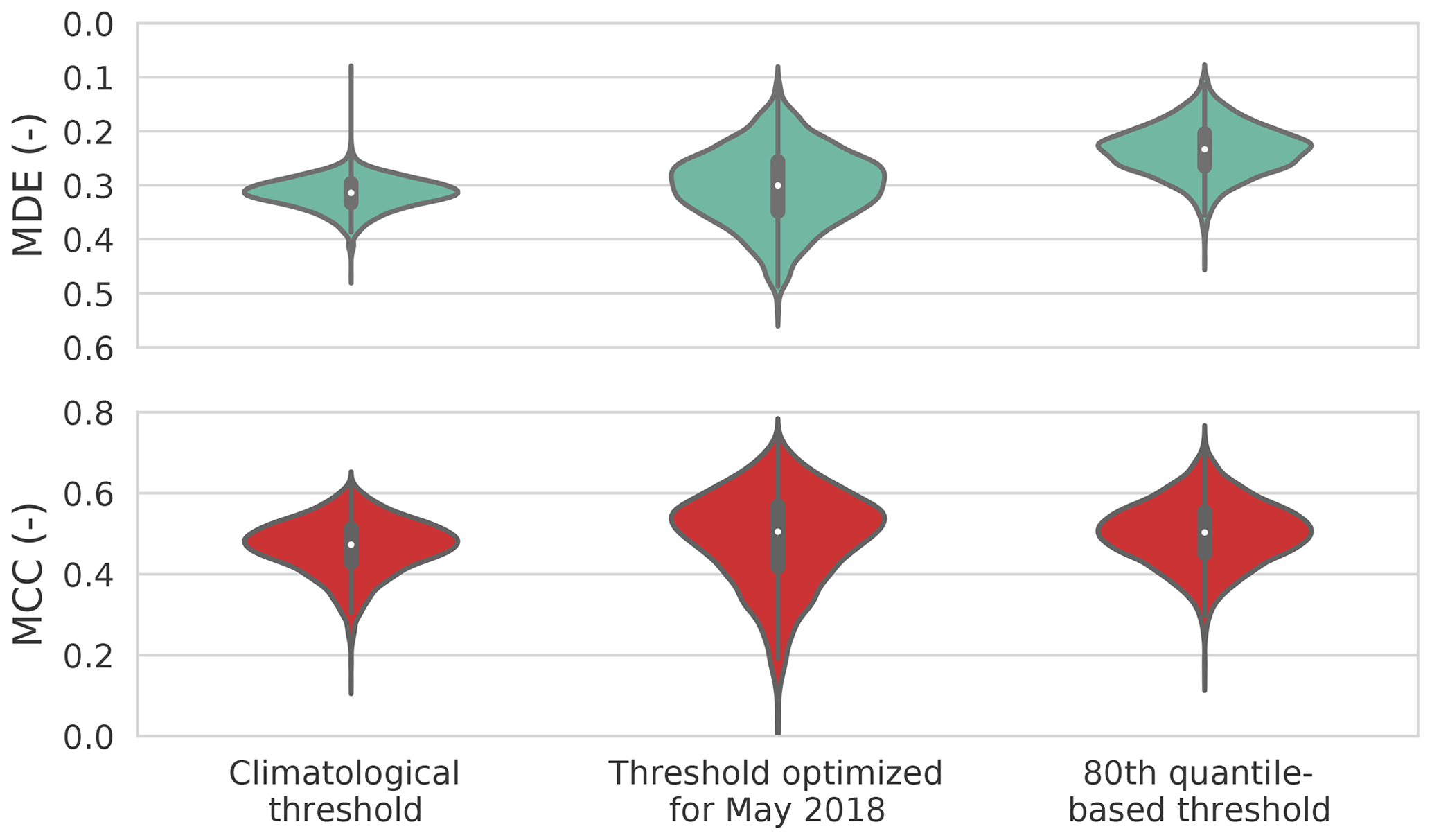
Figure 4 Mean detection error (MDE) and the Matthews correlation coefficient (MCC) for three rain event detection schemes for the whole analysis period.

When we optimized the threshold for each CML for May 2018 and then applied these thresholds for the whole period, the performance increased with a median MDE of 0.32 and a median MCC of 0.46. The better performance of the MDE and MCC values highlights the importance of a specific threshold for each individual CML, accounting for their individual tendency to fluctuate. Nevertheless, the range of MDE and MCC values is wider than with the climatological threshold. The wider range of MDE and MCC values, however, indicates that there is also a need to adjust the individual thresholds over the course of the year.

The 80th quantile-based method had the lowest median MDE (0.27) and highest median MCC (0.47). Therefore, it misclassified the least wet and dry periods compared with the other methods.

The threshold, which is based on the 80th quantile, is independent of climatology and depends on the individual tendency of a CML to fluctuate. Although the factor used to scale the threshold was derived from comparison with the reference data set, as described in Sect. 3.2.2, it was stable over all seasons and for CMLs in different regions of Germany. Validating the scaling factor with other CML data sets could be a promising method for data-scarce regions, as no external information is needed.

For single months, the MDE was below 0.20, as shown in Table 2, which still leaves room for an improvement of this rain event detection method. Enhancements could be achieved by adding information from nearby CMLs, if available. Moreover, data from geostationary satellite could be used. Schip et al. (2017) found improvements of the rain event detection when using rainfall information from the Meteosat Second Generation (MSG) satellite, which carries the Spinning Enhanced Visible and InfraRed Imager (SEVIRI) instrument.

All further processing, presented in the next sections, uses the method based on the 80th quantile.

4.2 Performance of wet antenna attenuation schemes

Two WAA schemes are tested and adopted for the present CML data set. Both are compared with the uncorrected CML data and the reference in Fig. 5. Without a correction scheme, the CML-derived rainfall overestimated the reference rainfall by a factor of 2 when considering mean hourly rain rates, as displayed in Fig. 5a. The correction by Schleiss et al. (2013) produced comparable mean hourly rain rates with respect to the reference data set. Despite its apparent usefulness in compensating for WAA, this scheme only worked well for stronger rain events. The mean detection error is higher than for the uncorrected data set, because small rain events are suppressed completely throughout the year. The discrepancy can also be a result of the average path length of 7.6 km in our data set which is 4 times the length of the CML Schleiss et al. (2013) used. This might have an impact, as shorter CMLs have a higher likeliness that both antennas get wet. Furthermore, the type of antenna and antenna cover impacts the wetting during rain, as discussed in section Sect. 3.2.3.

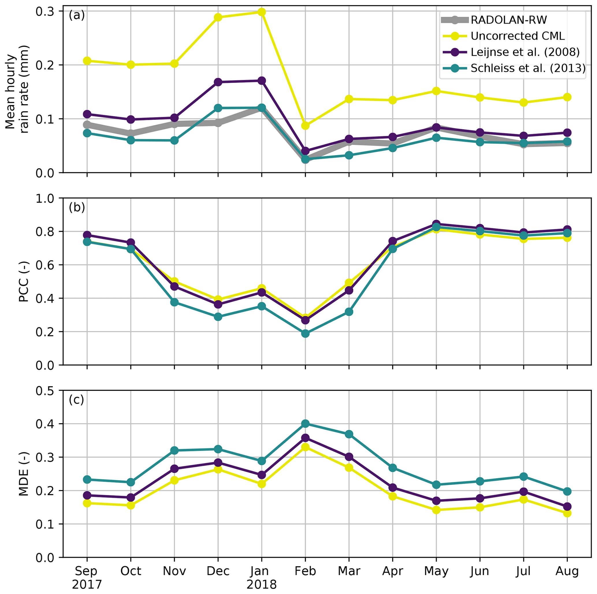
Figure 5 Wet antenna attenuation compensation schemes compared with respect to their influence on the (a) mean hourly rain rate, (b) the correlation between the derived rain rates and the reference, and (c) the mean detection error between the derived rain rates and the reference.

Using the method of Leijnse et al. (2008), the overestimation of the rain rates was also well compensated for. It incorporates physical antenna characteristics and, more importantly, depends on the rain rate. The higher the rain rate, the higher the WAA compensation. This leads to less suppression of small events. The MDE is close to the uncorrected data sets, and the PCC is higher, as displayed in Fig. 5b and c. Recent results from Fencl et al. (2019) also favor a dynamic, rain-intensity-dependent WAA model instead of a constant value for WAA compensation. Therefore, the scheme from Leijnse et al. (2008) is used for the evaluation of the CML-derived rain rates in the following sections.

Both methods are parameterized, neglecting known and unknown interactions between WAA and external factors like temperature, humidity, radiation, and wind. Current research aims to close this knowledge gap, but the feasibility for large-scale networks such as the one presented in this study is going to be a challenge as only TSL and RSL are available. A possible solution is the WAA model based on the reflectivity, efficiency, and directivity of the antenna proposed by Moroder et al. (2020), which would have to be measured by future CML hardware. Another approach could be to extend the analysis using meteorological model reanalysis products in order to better understand WAA behavior in relation to meteorologic parameters like wind, air temperature, humidity, and solar radiation.

4.3 Evaluation of CML-derived rainfall

Path-averaged rainfall information obtained from almost 4000 CMLs is evaluated against a reference data set, RADOLAN-RW. In Fig. 6, we show scatter density plots of path-averaged hourly rain rates, daily rainfall sums, and seasonal sums of each CML with the respective performance measures. Furthermore, scatter density plots of hourly, path-averaged rain rates and rain rates from interpolated rainfall maps are compared for each month in Figs. 8 and 9.

Looking at the differences between the seasons in Fig. 6, it is evident that CMLs are prone to producing a significant rainfall overestimation during the cold season (December–January–February; DJF). This can be attributed to precipitation events with melting snow that mainly occur from November to March. Melting snow can potentially cause as much as 4 times higher attenuation than a comparable amount of liquid precipitation (Paulson and Al‐Mreri, 2011). Snow, ice, and their melt water on the covers of the antennas can also cause additional attenuation. A decrease in the seasonal performance measures also reflects this effect, as the lowest values for PCC and highest values for CV, MAE, RMSE, bias, and MDE are found for DJF. The largest overestimation occurs at low reference rain rates. At higher reference rain rates, which are most likely those stemming from liquid precipitation, there is far less overestimation. In spring (March–April–May; MAM) and fall (September–October–November; SON), overestimation by CML rainfall is still visible, but it is less frequent. This can be explained by the fact that snowfall can occur from October to April in the Central German Upland and the Alps. The best agreement between CML-derived rainfall and RADOLAN-RW is found for the summer months (June–July–August; JJA).

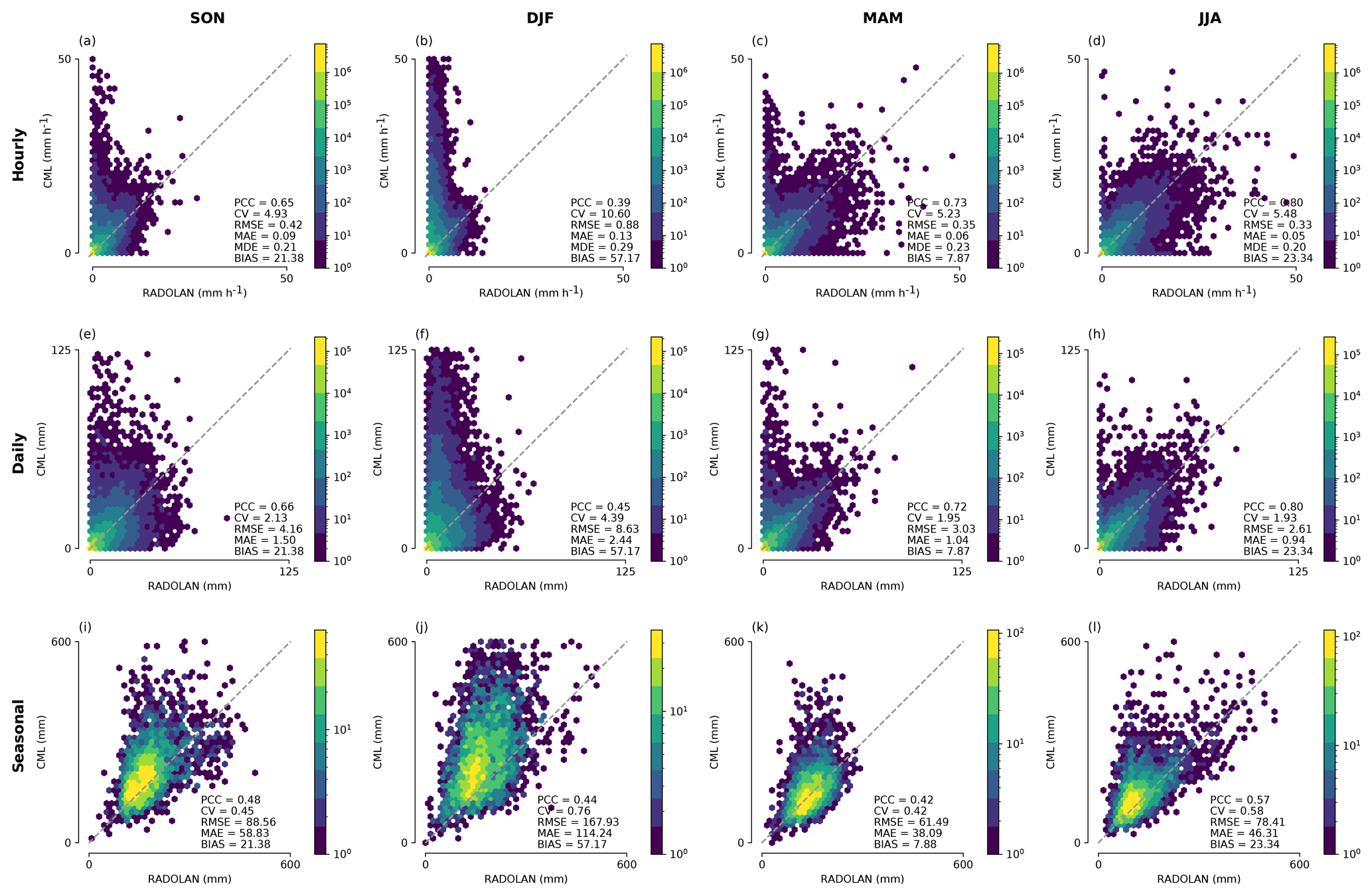
Figure 6 Seasonal scatter density plots of CML-derived rainfall and path-averaged RADOLAN-RW data for hourly (a–d), daily (e–h), and seasonal (i–l) aggregations with the respective performance metrics calculated from all available data pairs.

The temporal aggregation to daily rainfall sums and the respective performance measures are shown in Fig. 6e–h. The general relation between CML-derived rainfall and the reference is similar on both the hourly and daily scales. The bias is identical for the daily aggregation. The RMSE and MAE are higher due to the higher rain sums. The overestimation during the winter month is unchanged.

The accumulated rainfall sums of individual CMLs are compared against the reference rainfall accumulation for each season in Fig. 6i–l. The overestimation of the CML-derived rainfall sums in DJF, and partly SON and MAM, can again be attributed to the presence of non-liquid precipitation. This overestimation is larger for higher rainfall sums. This could be the result of more extensive snowfall in the mountainous parts of Germany, which are also the areas with the highest precipitation year round. Rainfall sums close to zero could be the result of the quality control that we applied, because periods with missing data in CML time series are consequently not counted in the reference rainfall data set. Therefore, the rainfall sums in Fig. 6 are not representative of the rainfall sum over Germany for the period shown. The PCC values for the four seasons shown in Fig. 6i–l range from 0.42 in MAM to 0.57 in JJA.

4.4 Performance measures for different subset criteria

Table 2 gives an overview of the monthly performance measures for different subsets of CML-derived and path-averaged reference rainfall. In the following, we will discuss the effects of the different subset criteria and then compare our results to previous CML rainfall estimation studies.

For all subset criteria, the best performance measures are found during late spring, summer, and early fall. The highest PCC values are reached when all data pairs, including true dry events, are used to calculate the measures. When very light rain (<0.1 mm h⁻¹) is set to zero on an hourly basis, the performance measures stay very similar, with the exception of the CV and bias, which show a slight increase in performance. This means that even when very small rain rates <0.1 mm are produced, they do not change rainfall sums too much.

When either R_CML or R_reference exceed 0 mm h⁻¹, the performance measures are worse than with all data because all 0 mm h⁻¹ pairs are removed. When the same subset criterion is set to 0.1 mm h⁻¹, good agreement in the range of very small rain rates below 0.1 mm h⁻¹ between both data becomes apparent because the performance measures get worse without them.

To examine the performance of the CML-derived rainfall during rain events detected by the reference, two thresholds are selected, where the reference must be above 0.1 and 1 mm h⁻¹, respectively, for the period to be considered rainy. Using these thresholds, all false wet classifications are removed before the calculation of the performance measures. The PCC values with these thresholds are still high for the non-winter months. The CV is reduced, whereas the MAE and RMSE are higher due to higher mean rain rates. The biggest differences can be observed in the bias, where the influence of false wet detection and the overestimation of CMLs over 0.1 and 1 mm h⁻¹ reduce the bias.

de Vos et al. (2019)Rios Gaona et al. (2015)

Table 3 Comparison of the performance measures to similar CML validation studies (only link-based comparisons) with respective thresholds.

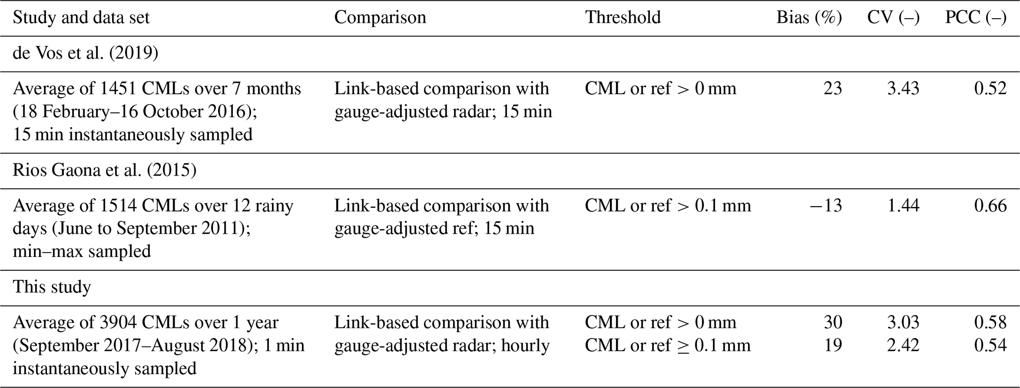
Therefore, when discussing these performance measures in relation to previous studies on CML rainfall estimation, the selection of the threshold is of great importance. A study by de Vos et al. (2019) shows a collection of Dutch CML-studies (their Table A1). In Table 3, we compare our performance measures to those of studies shown in de Vos et al. (2019) that are similar to our study. “Similar” in this context means considering the size and temporal aggregation of the CML data set as well as the use of radar data as a reference for path-averaged (link-based) rain rates from CMLs. The performance measures from our results with the respective thresholds are in the same range as the performance measures from de Vos et al. (2019) and Rios Gaona et al. (2015). Nevertheless, the results should not be compared in a purely quantitative way, because both use different sampling strategies and span different time periods.

4.5 Rainfall maps

Interpolated rainfall maps of CML-derived rainfall compared to RADOLAN-RW are shown in Figs. 7, 8, and 9. The respective CML maps have been derived using inverse distance weighting (IDW) with the RADOLAN-RW grid as the target grid and on an hourly basis. Each CML rainfall value is represented as one synthetic point observation at the center of the CML path. For each pixel of the interpolated rainfall field, the nearest 12 synthetic CML observation points are taken into account. Weights decrease with the distance d (in km), according to d⁻². After the interpolation, we masked out grid cells more than 30 km from a CML path for each individual time step. Hence, hourly rainfall maps derived from CMLs are only produced for areas with data coverage. We applied the same mask to the reference data set on an hourly basis to increase the comparability between both data sets. For the aggregated rainfall maps, we summed up the interpolated, individually masked, hourly rainfall fields. As an example, Fig. 7 shows 48 h of accumulated rainfall in May 2018. The general distribution of CML-derived rainfall reproduces the pattern of the reference very well, and the rainfall sums of both data sets are similar. However, individual features of the RADOLAN-RW rainfall field are missed due to the limited coverage of CMLs in certain regions. A video of this 48 h showcase with hourly time steps is published alongside this study (Graf et al., 2020).

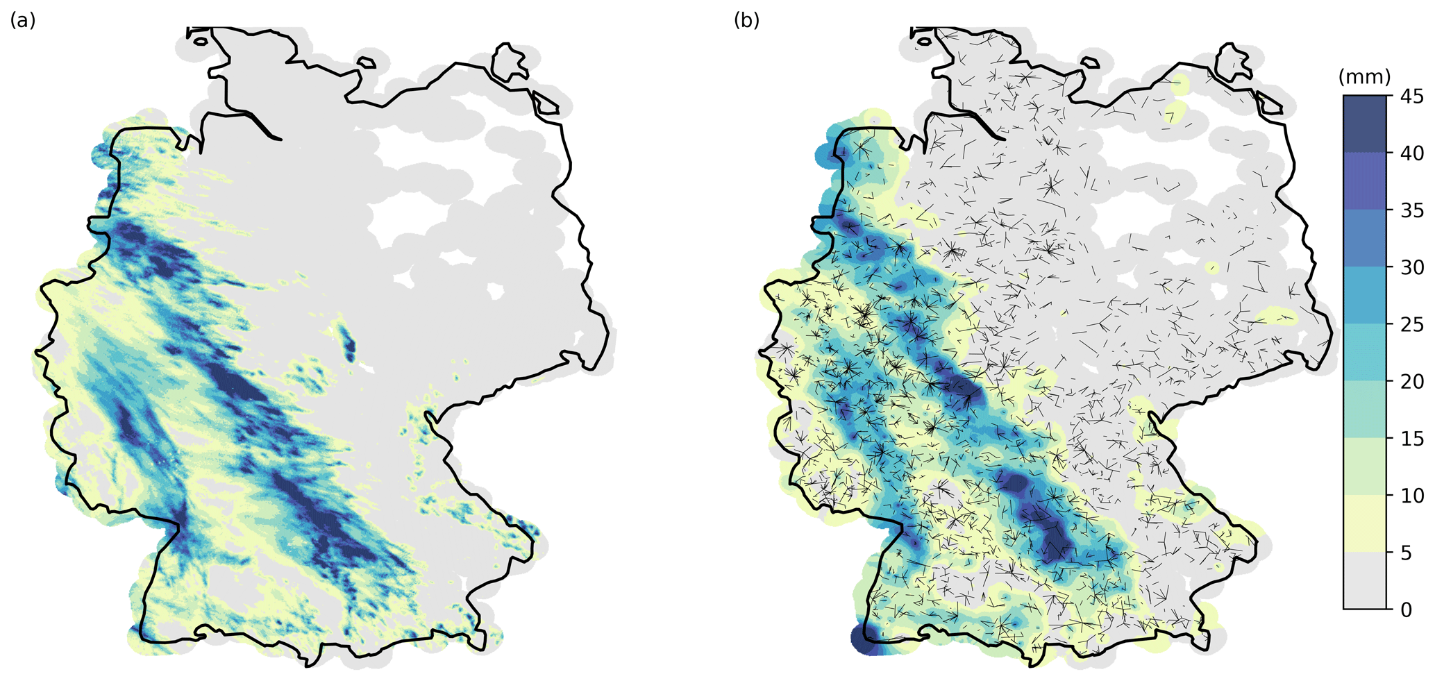
Figure 7 Accumulated rainfall for a 48 h showcase from 12 to 14 May 2018 for (a) RADOLAN-RW and (b) CML-derived rainfall. CML-derived rainfall is interpolated using a simple inverse distance weighting interpolation. A coverage mask of 30 km around CMLs is used. This showcase is visualized in a video supplement with an hourly resolution (Graf et al., 2020).

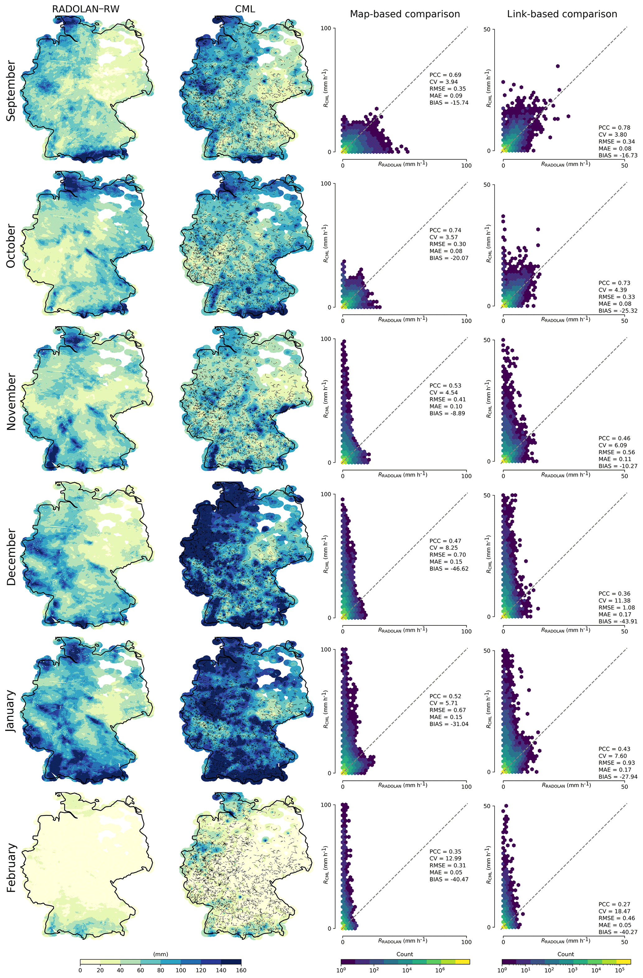
Figure 8 Monthly aggregations of hourly rainfall maps from CMLs compared to RADOLAN-RW from September 2017 to February 2018. For each month, two scatter density plots are shown: one for pixel-by-pixel comparison of the hourly maps (map-based comparison), and one for the comparison of the hourly path-averaged rainfall along the individual CMLs (link-based comparison).

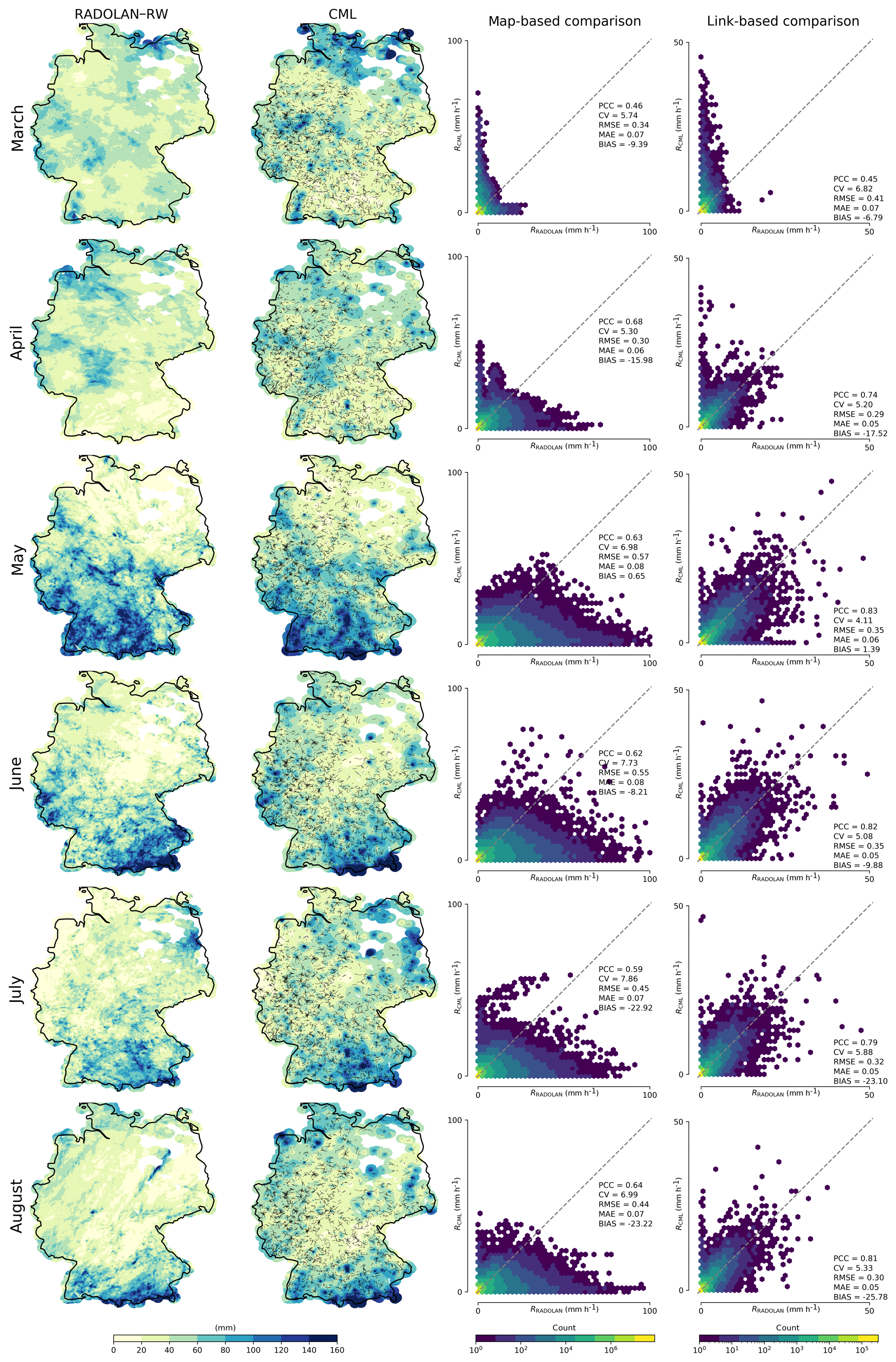
Figure 9 Monthly aggregations of hourly rainfall maps from CMLs compared to RADOLAN-RW from March to August 2018. For each month, two scatter density plots are shown: one for pixel-by-pixel comparison of the hourly maps (map-based comparison), and one for the comparison of the hourly path-averaged rainfall along the individual CMLs (link-based comparison).

A qualitative comparison of monthly aggregation of the hourly rainfall maps is shown in Figs. 8 and 9. The CML-derived rainfall fields resemble the general patterns of the RADOLAN-RW rainfall fields. Summer months show better agreement than winter months. This is a direct result of the decreased performance of CML-derived rain rates during the winter season, as explained in Sect. 4.3. Strong overestimation is also visible year round for a few individual CMLs, for which the filtering of erratic behavior was not successful.

A quantitative comparison of the CML-derived rainfall maps to the reference is shown in the third column of Figs. 8 and 9. For these scatter density plots, we used all hourly pixel values of the respective month within the 30 km coverage mask. During the winter month, CMLs show strong overestimation. This is a direct result of non-liquid precipitation, as described in Sect. 4.3. From May to August 2018, the reference shows very high rain intensities between 50 and 100 mm h⁻¹, which are not produced by the CML rainfall maps.

This can be attributed to several reasons. First, CML-derived rainfall, which serves as a basis for the interpolation, is path-averaged, with a typical path length from 3 to 15 km. This means that the rainfall estimation of a single CML represents an average of several RADOLAN-RW grid cells which smoothes out the extremes. Second, due to the interpolation, rainfall maxima in the CML rainfall maps can only occur at the synthetic observation points at the center of each CML. Third, rainfall is only observed along the path of CMLs, and, even with almost 4000 CMLs across Germany, the spatial variation of rainfall cannot be fully resolved. In particular in summer, small convective rainfall events might not intersect with CML paths and, hence, cannot appear in the CML-derived IDW interpolated rainfall fields.

Considering this, the effect of different coverage ranges around the CMLs has to be taken into account. For the map-based comparison in Figs. 8 and 9, we tested several distances from 10 to 50 km. For the results presented, we choose 30 km as a trade-off between minimizing the uncertainty of the spatial interpolation and the goal of reaching countrywide coverage with the produced rainfall maps. The study by van de Beek et al. (2012) found an averaged range of around 30 km for summer semivariograms of 30 years of hourly rain gauge data in the Netherlands, which can be used to justify and enforce our choice.

With a 10 km coverage range, the performance measures are better than those for 30 km, which are shown in Figs. 8 and 9. Monthly PCC values show an increase of around 0.05, and the bias is reduced by 3 % to 5 %. Nevertheless, with a coverage of 10 km around the CMLs, coverage gaps emerge not only in the northeastern part of Germany but also in the southeastern part. In contrast, with a 50 km coverage range, the countrywide coverage is almost given, although the performance measures are worse compared with 30 km (PCC shows a decrease of between 0.03 and 0.05). Overall, the difference in the performance measures of the 10 and 50 km coverage masks is limited by the high density of CMLs in most parts of Germany, which already led to an almost full coverage with the 10 km mask.

In order to highlight the differences between a map-based and link-based comparison, Figs. 8 and 9 also show hourly link-based scatter density plots for each month. The differences in the performances measures for the warm months support the qualitative impression that the map-based comparison does not perform as well. The interpolation is prone to introducing an underestimation for areas that are more distant from the CML observations. During the winter months, this underestimation compensates for the overestimation of the individual CMLs due to wet snow and ice-covered antennas. Hence, because the two errors compensate for each other by chance, this results in slightly better map-based performance measures compared with the link-based measures for the winter months. Nevertheless, rainfall estimation using CMLs for months with non-liquid precipitation is considerably worse than for summer months in all spatial and temporal aggregations.

The derivation of spatial information from the estimated path-averaged rain rates could be improved by applying more sophisticated techniques, as described in Sect. 1. We have already carried out several experiments using kriging in order to test one of these potential improvements over IDW. We followed the approach of Overeem et al. (2016b) and adjusted the semivariogram parameters on a monthly basis based on the values from van de Beek et al. (2012). We also tried fixed semivariogram parameters and parameters estimated from the individual CML rainfall estimates for each hour. However, in conclusion, we only found marginal improvements or no improvement of the performance metrics of the CML rainfall maps. This, combined with the drawback of kriging that the required computation time is significantly increased (approximately 10 to 100 times slower than IDW, depending on factors such as the number of neighboring points used by a moving kriging window), meant that we decided to keep using the simple – yet robust and fast – IDW interpolation. Furthermore, it is important to note that the errors in rain rate estimation for each CML contribute most to the uncertainty of CML-derived rainfall maps (Rios Gaona et al., 2015). Hence, within the scope of this work, we focused on improving the rainfall estimation at the individual CMLs.

Considering that we use a reference data set derived from 17 C-band weather radars combined with more than 1000 rain gauges for our comparison, the similarity with the CML-derived maps, which solely stem from the opportunistic usage of attenuation data, is remarkable.

5 Conclusions

German-wide rainfall estimates derived from CML data compared well with RADOLAN-RW, a hourly gridded gauge-adjusted radar product from the DWD. The methods used to process the CML data showed promising results over 1 year and several thousand CMLs across all landscapes in Germany, except for the winter season.

We presented the data processing of almost 4000 CMLs with a temporal resolution of 1 min from September 2017 to August 2018. We developed a parallelized processing work flow that could handle the size of this large data set. This workflow enabled us to test and compare different processing methods over a large spatiotemporal scale.

A crucial processing step is the rain event detection from the TRSL, which is the raw attenuation data recorded for each CML. We used a scheme from Schleiss and Berne (2010) that utilizes the 60 min rolling standard deviation (RSD) and a threshold. We derived this threshold from a fixed multiple of the 80th quantile of the RSD distribution of each TRSL. Compared with the original threshold using the 95th quantile, which is based on rainfall climatology, the 80th quantile reflects the general tendency of each CML's TRSL to fluctuate. We were able to reduce the amount of misclassification of wet and dry events, reaching a yearly average MDE of 0.27, with a MDE for the summer months below 0.20. A potential approach to further decrease the amount of misclassifications could be the use of additional data sets. For example, cloud cover information from geostationary satellites could be employed to reduce false wet classification, by (as a first simple approach) defining periods without clouds as dry. Another opportunity might be additionally implementing algorithms exploiting information from neighboring CMLs.

To compensate for WAA (the attenuation caused by water droplets on the cover of CML antennas), we compared and adjusted two approaches from the literature. In order to evaluate WAA compensation approaches, we used the reference data set. We were able to reduce the overestimation caused by WAA, while maintaining the detection of small rain events, using an adjustment of the approach introduced by Leijnse et al. (2008). The compensation for WAA without evaluation against a reference data set is not feasible with the CML data set we use.

Compared to the reference data set (RADOLAN-RW), the CML-derived rainfall performs well for periods with liquid precipitation alone. For winter months, the performance of CML-derived rainfall is limited. Melting snow and snowy or icy antenna covers can cause additional attenuation, resulting in the overestimation of precipitation, whereas dry snow cannot be measured at the frequencies and the TRSL quantizations that the CMLs in our data set use. We found high correlations for hourly, monthly, and seasonal rainfall sums between CML-derived rainfall and the reference. To increase the comparability of our analysis with existing and future studies on CML rainfall estimation, we calculated all performance metrics for different subset criteria (e.g., requiring that either CML or reference rainfall is larger than 0 mm).

We found the performance measures of this study to be in accordance with similar CML studies, although the comparability is limited due to differences in the CML and reference data sets. CML-derived rainfall maps calculated with a simple yet robust IDW interpolation showed the plausibility of CMLs as a stand-alone rainfall measurement system.

With the analysis presented in this study, the need for reference data sets in the processing routine of CML data is reduced; thus, the opportunistic sensing of countrywide rainfall with CMLs is at a point, where it should be transferable to (reference) data-scarce regions. Especially in Africa, where water availability and management are critical, this task should be challenged, as in Doumounia et al. (2014). The high temporal resolution of the data set presented can be used in future studies, such as those focusing on urban water management. In addition, CML-derived rainfall can also be used to complement other rainfall data sets; for example, it can be utilized to improve the radar data adjustment in RADOLAN-RW in regions with high CML density and regions, like mountain ranges, where radar data are often compromised. Thus, CMLs can contribute substantially to improving the spatiotemporal estimations of rainfall.

Appendix A

Schleiss and Berne (2010)Leijnse et al. (2008)Leijnse et al. (2008)Schleiss and Berne (2010)Schleiss et al. (2013)Schleiss et al. (2013)

Table A1 A comprehensive overview of the parameters used, a short description, and their reference from the literature (if applicable). Parameters with enumeration in parentheses were not used in the final processing.