the Creative Commons Attribution 4.0 License.
the Creative Commons Attribution 4.0 License.
 | 26 May 2020
Uncovering the shortcomings of a weather typing method
Els Van Uytven
Jan De Niel
Patrick Willems
In recent years many methods for statistical downscaling of the precipitation climate model outputs have been developed. Statistical downscaling is performed under general and method-specific (structural) assumptions but those are rarely evaluated simultaneously. This paper illustrates the verification and evaluation of the downscaling assumptions for a weather typing method. Using the observations and outputs of a global climate model ensemble, the skill of the method is evaluated for precipitation downscaling in central Belgium during the winter season (December to February). Shortcomings of the studied method have been uncovered and are identified as biases and a time-variant predictor–predictand relationship. The predictor–predictand relationship is found to be informative for historical observations but becomes inaccurate for the projected climate model output. The latter inaccuracy is explained by the increased importance of the thermodynamic processes in the precipitation changes. The results therefore question the applicability of the weather typing method for the case study location. Besides the shortcomings, the results also demonstrate the added value of the Clausius–Clapeyron relationship for precipitation amount scaling. The verification and evaluation of the downscaling assumptions are a tool to design a statistical downscaling ensemble tailored to end-user needs.
- Article
(1908 KB) - Full-text XML
- BibTeX
- EndNote


For a 1.5 ∘C temperature rise, the worldwide direct flood damage is estimated to increase by 160 %–240 % (Dottori et al., 2018). To minimise that potential impact, our society opts for two complementary strategies, namely climate mitigation and climate adaptation (Stocker et al., 2013). Consequently, vulnerability, impact and adaptation studies find ground in our society (Alfieri et al., 2016; Åström et al., 2016; Brekke et al., 2009; Termonia et al., 2018; Vansteenkiste et al., 2014; Willems, 2013b). These studies require projected hydrometeorological time series and use the output of global climate models as primary information. However, the direct application of this output for impact modelling is hindered by climate model biases (Kotlarski et al., 2014; Tabari et al., 2016), the mismatch in temporal and spatial resolutions between the climate model output, and the time series required for impact modelling (Cristiano et al., 2018; Salvadore et al., 2015). Therefore, statistical downscaling or dynamical downscaling is applied. The statistical downscaling approach bridges the resolution gap through statistical relationships between the predictors and predictand, whereas in the dynamical downscaling approach regional climate models (RCMs) and limited area climate models (LAMs) are developed. Despite the refined resolution of RCMs and LAMs, their climate model output remains biased and requires bias correction (Ehret et al., 2012; Maraun, 2016; Teutschbein and Seibert, 2012). Both downscaling approaches have strengths and shortcomings arising from their underlying assumptions (Casanueva et al., 2016; Flaounas et al., 2013; Le Roux et al., 2018; Maraun et al., 2010; Vaittinada Ayar et al., 2016).
The statistical downscaling approach builds on four general assumptions (Benestad et al., 2008; Maraun et al., 2010; Maraun and Widmann, 2018; Schoof, 2013) as follows:
-
The relationship between the predictors and the predictand is relevant (referred to as the informative assumption). This is of importance in the development of new statistical downscaling methods (SDMs), which requires the selection of predictors (Fu et al., 2018; Sachindra et al., 2018; Wilby and Wigley, 2000; Yang et al., 2017). The selected predictors should relate to the physical processes explaining the predictand changes. Precipitation, more specially, responds to large-scale atmospheric circulation and thermodynamic laws (Emori and Brown, 2005; Kröner et al., 2017; Santos et al., 2016) and, hence, sea level pressure, geopotential height, relative humidity, and/or (dew point) temperature are common predictors (Maraun and Widmann, 2018).
-
The predictors are adequately and accurately simulated by the climate model runs (referred to as the perfect prognosis assumption). The evaluation of this assumption is foremost performed under the name bias analysis. The bias in the predictors depends on, among others, the model resolution, parameterisation schemes, internal variability, and the choice of the reference period (Anstey et al., 2013; Arakawa, 2004; Davini et al., 2017; Deser et al., 2012; Fadhel et al., 2017; Hartung et al., 2017; Prein et al., 2015; Rybka and Tost, 2014; Tabari et al., 2016; Vanden Broucke et al., 2018; Watterson et al., 2014).
-
The relationship between the predictors and the predictand remains time-invariant (referred to as the the stationarity assumption). This means that the relationship between the predictors and the predictand, which has been established by using historical observations, remains applicable under climatic changes. Of all the assumptions, this assumption is the most difficult one to validate as no future observations are available yet (Dixon et al., 2016; Lanzante et al., 2018; Salvi et al., 2016; Wang et al., 2018).
-
The predictand is sensitive to the greenhouse gas scenarios. Schoof (2013) has pointed out that one predictor variable could strongly respond to the greenhouse gas scenarios while another variable would not. This observation is, for instance, applicable to changes in temperature and mean sea level pressure respectively. Moreover, due to the internal variability of the climate system and the climate-model-related uncertainties, the response of the predictor to the greenhouse gas scenarios is often masked (Van Uytven and Willems, 2018). Hence, the response of the predictand to the greenhouse gas scenarios is governed by a smart choice of predictors.
Alongside the general statistical downscaling assumptions, each SDM has method specific or structural assumptions. They are encapsulated in the downscaling methodology, create the method strengths and limitations, and are responsible for the statistical downscaling uncertainty contribution. An overview of commonly applied SDMs for precipitation downscaling and their strengths and limitations is provided by Hewitson et al. (2014), Maraun et al. (2010), Maraun and Widmann (2018), and Sunyer et al. (2015).
The main objective of this paper is to simultaneously verify and evaluate the general and structural statistical downscaling assumptions. Most studies address the general and structural statistical downscaling assumptions independently. Hence, there are studies addressing one or some of the general statistical downscaling assumptions (Dixon et al., 2016; Fu et al., 2018; Haberlandt et al., 2015; Hertig et al., 2017; Mendoza et al., 2016; Merkenschlager et al., 2017; Salvi et al., 2016; Tabari et al., 2016), and there are other studies addressing the structural assumptions by the statistical downscaling of surrogate climate model runs (Bürger et al., 2012; Gutmann et al., 2014; Hertig et al., 2018; Maraun et al., 2018; Roberts et al., 2019; Werner and Cannon, 2016; Widmann et al., 2019; Yang et al., 2019), or by the statistical downscaling of the projected climate model output (Li et al., 2017; Sørup et al., 2018; Sunyer et al., 2015; Vaittinada Ayar et al., 2016; Wang et al., 2016; Wootten et al., 2017). To objectively identify the shortcomings of statistical downscaling methods, the verification and evaluation of the general and structural assumptions should, however, be performed simultaneously. To the authors' knowledge, there are no papers yet which simultaneously address the verification of both types of assumptions.
In this paper, the verification and evaluation of the general and structural assumptions are illustrated for a weather typing (WT) SDM for the purpose of climate change impact modelling on precipitation in Belgium during winter (December to February). The studied WT SDM is the method labelled SD-B-7 by Willems and Vrac (2011). Downscaling is performed in three steps. In the first step, weather types are identified based on the mean sea level pressure patterns. In the second step, the relationship between the predictors (weather types) and predictand (point precipitation) is established by using analogues. In the last step, the precipitation amounts are scaled following the Clausius–Clapeyron (CC) relationship. Overall strengths emerge from the physical background of the SDM (Shepherd et al., 2018).
This paper is organised into the following sections. Section 2 introduces the studied SDM and the hydrometeorological data. Section 3 outlines the verification of the downscaling assumptions, and the corresponding results and discussions are included in Sect. 4. Section 5 summarises the main findings and makes suggestions for future research.
2.1 The weather typing method
The considered WT method is the method referred to as SD-B-7 by Willems and Vrac (2011). This method has been selected over the other WT methods as it accounts for both the changes in atmospheric circulation and the potential intensification of extreme precipitation due to temperature rise. The method downscales the daily gridded climate model output to a point time series with a time step equal to the observed time series by using a three-step approach. In the first step, the Jenkinson–Collison automated Lamb WT classification system is applied and the WTs are identified. In the second step, downscaled precipitation time series are produced by using WT analogues. In the last step, the precipitation amounts are scaled by using the Clausius–Clapeyron (CC) relationship.
2.1.1 Step 1: Jenkinson–Collison automated Lamb WT classification scheme
As shown in Fig. 1, a 16-point grid is centred around the study area. Assuming pi is the mean sea level pressure (MSLP) in point i of the 16-point grid and ψ the latitude of the study area, then the southerly flow (SF), westerly flow (WF), total flow (F), southerly shear vorticity (ZS), westerly shear vorticity (ZW), and total shear vorticity (Z) are calculated as follows (Jenkinson and Collison, 1977; Jones et al., 1993; Philipp et al., 2016):

Figure 1Spacing and numbering in the 16-point grid for the Jenkinson–Collison automated Lamb weather typing classification scheme.
The flow direction is based on an eight-direction compass (N – north; NE – northeast; E – east; SE – southeast; S – south; SW – southwest; W – west; and NW – northwest) and is calculated as follows:
If the outcome of Eq. (2) is positive, then 180∘ is added.
Based on a comparison of the flow indices and the flow direction, 27 different WTs are identified. The comparison of the flow indices considers the following criteria:
-
: pure directional WTs (W, NW, N, NE, E, SE, S, SW);
-
and Z>0: pure cyclonic WT (C);
-
and Z<0: pure anticyclonic WT (A);
-
and Z>0: hybrid cyclonic WTs (HCW, HCNW, HCN, HCNE, HCE, HCSE, HCS, HCSW);
-
and Z<0: hybrid anticyclonic WTs (HAW, HANW, HAN, HANE, HAE, HASE, HAS, HASW);
-
F<6 and Z<6: undefined WT (U).
These 27 WTs are regrouped to 11 WTs by equally dividing the hybrid WTs over the corresponding non-directional WTs (cyclonic or anticyclonic) and directional WTs. Although this might lead to information loss (Schiemann and Frei, 2010), it leads to larger sample sizes per WT and thus more accurate SDM relationships. The use of a reduced number of WTs is also in line with previous case studies for Belgium (Brisson et al., 2011; De Niel et al., 2017; Demuzere et al., 2009; Willems and Vrac, 2011).
2.1.2 Step 2: statistical downscaling by analogues
Downscaled time series are produced by finding analogues for the projected climate model output. In the first step, the bias in the number of wet days is removed by using a climate-model-dependent and a seasonally dependent wet-day threshold. In the next step, the downscaled precipitation time series are constructed by WT analogues.
The first criteria for defining an analogue wet day are the season and WT. Consider the day d of the projected climate model output, corresponding with the season s, WT wt and a daily precipitation amount p. Then, the search for an analogue day is conducted among the observed wet days in season s for which the WT equals wt. Besides the season and the WT, the exceedance probability of the daily precipitation amount p is considered. More precisely, the exceedance probability is calculated by using the total daily precipitation amounts of the wet days occurring in the season s and corresponding with the WT wt. As such, the analogue precipitation amount for day d equals the daily precipitation amount of the observed time series with the closest exceedance probability.
In case the observed precipitation time series has a sub-daily time step, the sub-daily precipitation amounts are aggregated to daily precipitation amounts. Next, for each season and WT, the exceedance probabilities for the observed daily precipitation amounts of wet days are calculated based on the total daily precipitation amount. After determining the analogue day, the sub-daily precipitation amounts of the analogue day are resampled to produce the downscaled time series.
2.1.3 Step 3: precipitation scaling by the Clausius–Clapeyron relationship
Besides large-scale circulation patterns, precipitation also responds to thermodynamic processes. The latter processes are accounted for by precipitation scaling following the CC relationship. The CC relationship describes the water-holding capacity in air masses, which more specifically increases by 7 % per degree of warming. Application of this scaling rate to precipitation intensities is valid assuming that extreme precipitation amounts are controlled by the local moisture availability and are not influenced by the large-scale atmospheric circulation patterns. In reality, however, physical processes interact and higher scaling rates are also found (Barbero et al., 2018; Blenkinsop et al., 2018; Manola et al., 2018; Lenderink et al., 2017; Zhang et al., 2017). The CC relationship is determined by the annual timescale. The temperature rise, to be applied for the CC scaling, is computed by using a seasonal quantile-based approach.
Although several studies have pointed out that dew point temperature is a better predictor for extreme precipitation amounts than the average daily temperature (Van de Vyver et al., 2019; Wasko et al., 2018), average daily temperatures were considered in this study due to their availability.
2.2 Meteorological data
For the main station of the Royal Meteorological Institute of Belgium (RMI) in Uccle, the precipitation and average temperature time series are available for the period 1901–2000 with a 10 min and daily time step respectively. The historical WTs are identified by using the daily gridded MSLP output for the EMULATE, ERA40 and NCEP/NCAR reanalysis data sets (Table 1). Hence, this study accounts for the recent findings of Horton and Brönnimann (2018) and Stryhal and Huth (2017). Both studies indicate that reanalysis data sets introduce uncertainties in the classification of WTs and the statistical downscaling step. By using daily WTs, rapidly occurring changes in the large-scale atmospheric circulation might be neglected (Åström et al., 2016). However, the winter season is of interest and for this season no rapidly evolving circulation changes, i.e. within 1 d, are expected.
Ansell et al. (2006)Uppala et al. (2005)Kalnay et al. (1996)Table 1Overview of the reanalysis data set ensemble employed in this study.
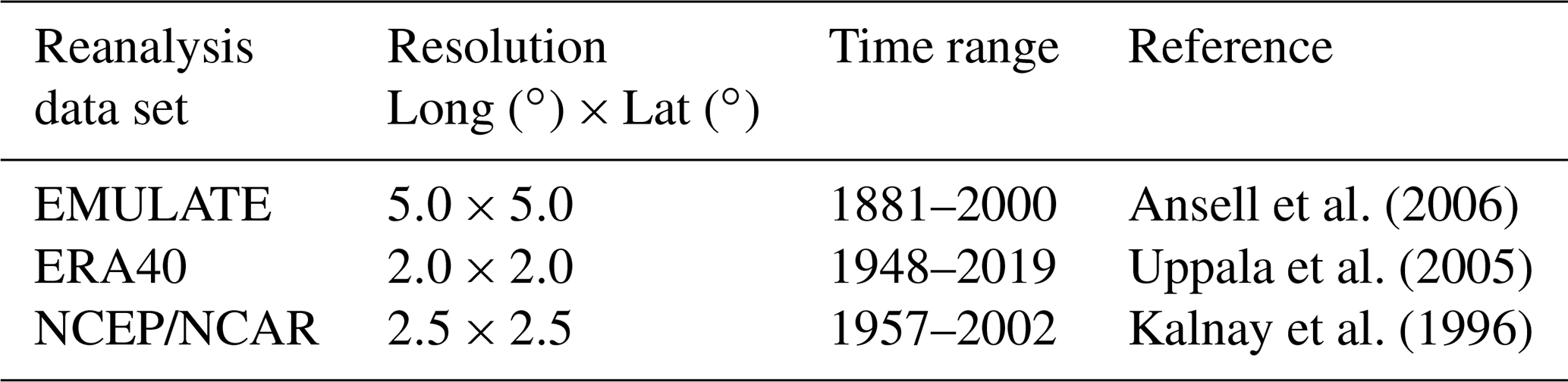
Table 2Overview of the climate model ensemble employed in this study.
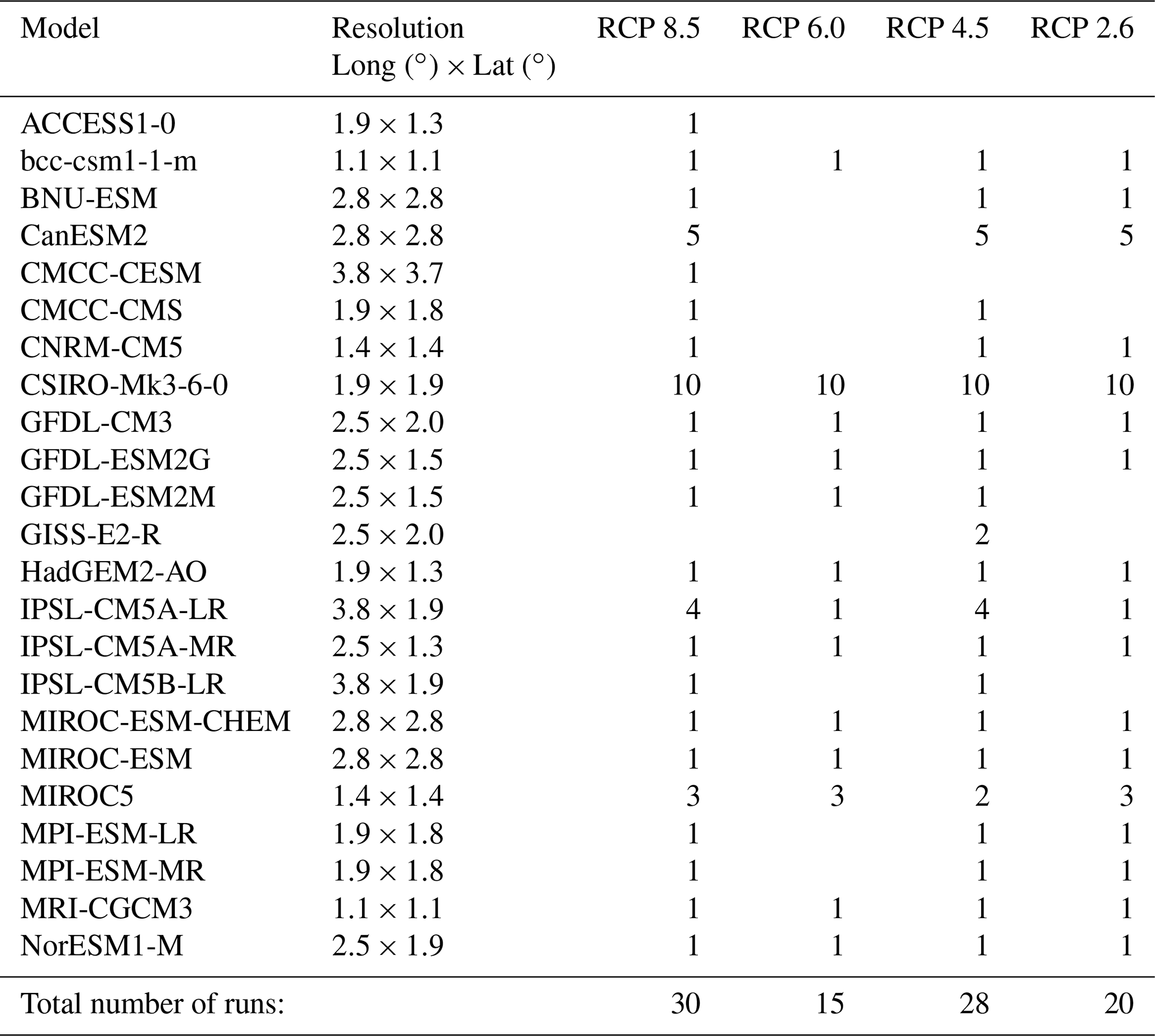
The climate model ensemble, presented in Table 2, includes 93 CMIP5 climate model runs of which 33 are control runs. For the climate change impact analysis, all four representative concentration pathways (RCPs) are considered, where the RCP 2.6, 4.5, 6.0, and 8.5 sub-ensembles include 20, 28, 15, and 30 climate model runs respectively. For each climate model run, daily MSLP, precipitation and average temperature output are extracted for 1961–1990 (control period) and 2071–2100 (scenario period). The precipitation and temperature data are extracted for the grid cell covering Uccle, whereas MSLP, required for the WT identification, is extracted for a larger area covering Uccle by using the 16-point grid of the WT classification system (Fig. 1).
The verifications of following assumptions are performed for the winter season, including the months of December, January and February.
3.1 Informative assumption
The informative assumption defines the existence of an informative and physically based relationship between the predictors and predictand. The predictors of the WT method are the average daily temperatures and WTs.
In order to examine the informative assumption for the WTs, the WT occurrences and the precipitation statistics related to the individual WTs are determined for the period 1961–1990. The studied precipitation statistics involve the precipitation accumulation, the number of wet days and the empirical distribution of independent extreme precipitation amounts. The independent 10 min, hourly and daily precipitation amounts are determined by using a peak-over-threshold method, setting the threshold at 0.1 mm h−1, and defining at least 12 h between successive events (Willems, 2000).
In order to examine the informative assumption for the average daily temperatures, the existence of the CC relationship is verified. The independent precipitation amounts are determined by using the 10 min precipitation amount time series and the daily average temperature time series between 1901 and 2000. First, the 10 min precipitation events in the time series are identified by using a peak-over-threshold method (threshold =0.1 mm h−1 and time between successive events >12 h). Next, the precipitation events and corresponding temperatures are classified in moving temperature bins and each bin is sorted from low to high (Manola et al., 2018). Finally, the magnification of the 90th, 95th and 99th percentile precipitation amount for increasing temperature bins is investigated.
3.2 Perfect prognosis assumption
The verification of the perfect prognosis assumption is especially of importance for the WT method. More specifically, the application of the WT analogues follows the principle of perfect prognosis methods. This means that a statistical relationship is first defined between observed predictors and observed predictand. Thereafter, the statistical relationship is applied to the projected climate model output. Consequently, the calibrated statistical relationship is not tailored to biases in the climate model output. The scaling of the precipitation amounts by the CC relationship, on the contrary, follows the principles of model output statistical methods. Those methods implicitly assume that the climate model biases are time-invariant and that through the application of changes the biases in the projected climate model output are cancelled by the biases in the historical climate model output.
The verification of the perfect prognosis assumption involves a comparison between the observed and simulated climate model WT occurrences. The verification is conducted over the period 1961–1990 by using the historical output of 33 global climate model runs (Table 2).
3.3 Stationarity assumption
To verify the stationarity assumption, the contributions of the dynamical and thermodynamic processes governing precipitation changes are studied over time. To this end, the observed period (1901–2000) is split into different sub-periods. The sub-periods are 20 years long and range between 1901 and 1920, 1921 and 1940, 1941 and 1960, 1961 and 1981, and 1981 and 2000. Each sub-period is thereafter considered as the scenario period for surrogate climate model runs. For instance, when 1901–1920 is selected as the scenario period, then the periods 1921–1940, 1941–1960, 1961–1981, and 1981–2000 act as control periods. When 1981–2000 is selected as the scenario period, then the periods 1901–1920, 1921–1940, 1941–1960, and 1961–1980 act as control periods. The combination of the different sub-periods yields an ensemble of 20 surrogate climate model runs. For each surrogate climate model run, the change in the average daily precipitation amounts of wet days is decomposed. More specifically, the precipitation amount changes ΔP are governed by the changes in the WT occurrence changes, i.e. the contribution by the dynamical processes ΔPdynamical, and thermodynamic, local, and/or mesoscale feedback changes, i.e. ΔPother (Souverijns et al., 2016). The contributions are calculated as follows:
with
-
Nj,contr the absolute occurrence frequency of wet days with WT j in the climate model output for the control period,
-
Nj,scen the absolute occurrence frequency of wet days with WT j in the climate model output for the scenario period,
-
Pj,contr the average daily precipitation amount of the wet days with WT j in the climate model output for the control period, and
-
Pj,scen the average daily precipitation amount of the wet days with WT j in the climate model output for the scenario period.
The decomposition is also performed by using the historical and projected output of the 93-member global climate model ensemble (Table 2).
3.4 Response to greenhouse gas scenarios
In order to verify the response of the predictand to the greenhouse gas scenarios, the WT method is applied to the output of 93 global climate model runs (Table 2). Next, the daily precipitation amounts for the downscaled time series are compared against the observed precipitation amounts and the intensification of the extreme precipitation amounts for increasing greenhouse gas scenarios is investigated. The intensification is visually inspected, and the focus is put on the magnification of the changes for increasing greenhouse gas scenarios. Furthermore, a comparison is made between the coarse global climate model changes and the changes for the downscaled time series. For sake of brevity, the changes in the 30-year return period and the average winter precipitation accumulation are investigated.
3.5 Structural downscaling assumptions
To investigate the added value of the CC relationship, the original SDM (with CC scaling) and the SDM without CC scaling are applied to the projected output of 93 global climate models (Table 2). The control period and the range of observations are defined as 1961–1990, and the scenario period is defined as 2071–2100. A comparison is made between the projected changes for the SDM with CC scaling and the SDM without CC scaling. The added value of the CC relationship is discussed in combination with the predictand response.
4.1 The informative assumption
Figure 2 presents the relative WT occurrence frequencies during the winter season. The results show that the A WTs occur most frequently and represent approximately 30 % of the winter days. Also the W, SW, and C WTs are identified as frequently occurring. The occurrence frequency of each of these WTs is approximately 12 %. Despite some details, there are no differences between the different reanalysis data sets. The WT occurrence patterns are generally in agreement with the recent findings of Otero et al. (2018). They identified the A WTs as the overall dominant winter WT in Europe. The A WTs, more specifically, represent on average 25 % of the winter days. The average occurrence frequency of the C WTs in Europe is estimated at approximately 15 %, the W WTs at approximately 8 %, and the SW at approximately 5 %. Note that the WT occurrences presented by Otero et al. (2018) have been averaged out over the European domain.
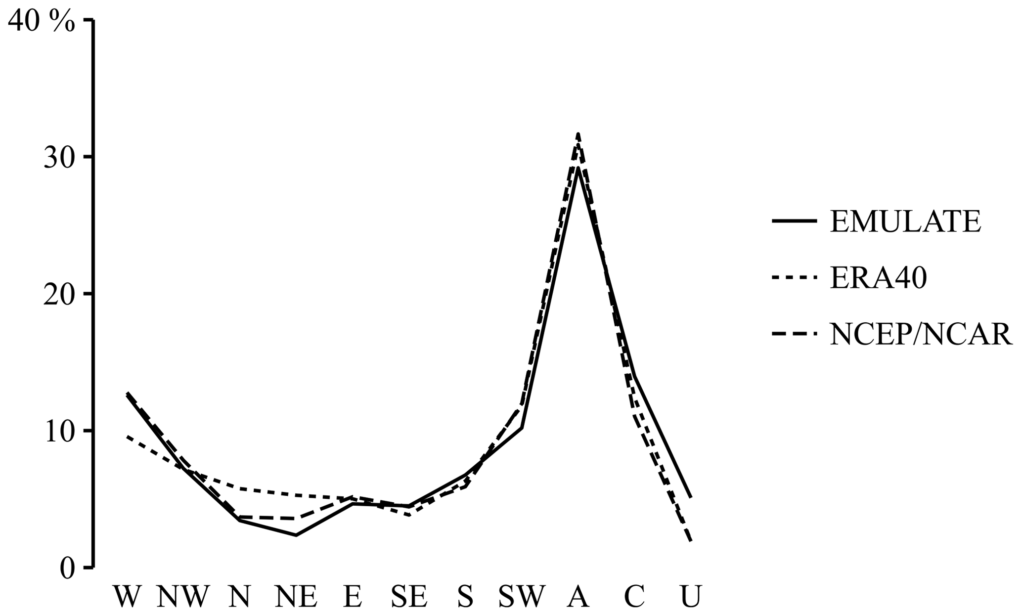
Figure 2Relative WT occurrence in the winter season for different reanalysis data sets. The results are obtained for the reference period 1961–1990.
Apart from the A WTs, the W, SW, and C WTs are associated with a high precipitation accumulation and together explain up to 71 % of the total winter precipitation accumulation (Appendix, Figs. A1 and A2). Additionally, these WTs are associated with higher precipitation amounts, as for instance shown for the NCEP∕NCAR reanalysis data set in Fig. 3. More specifically, the 1-year daily precipitation amount for the W WTs measures 0.51 mm h−1 and is twice as large as the corresponding amount for the A WTs, which measures 0.19 mm h−1. Also the NW WTs are characterised by higher precipitation amounts and a higher wet-day frequency. However, compared to the W, SW, and C WTs, their occurrence is rather low and contributes less to the precipitation accumulation.
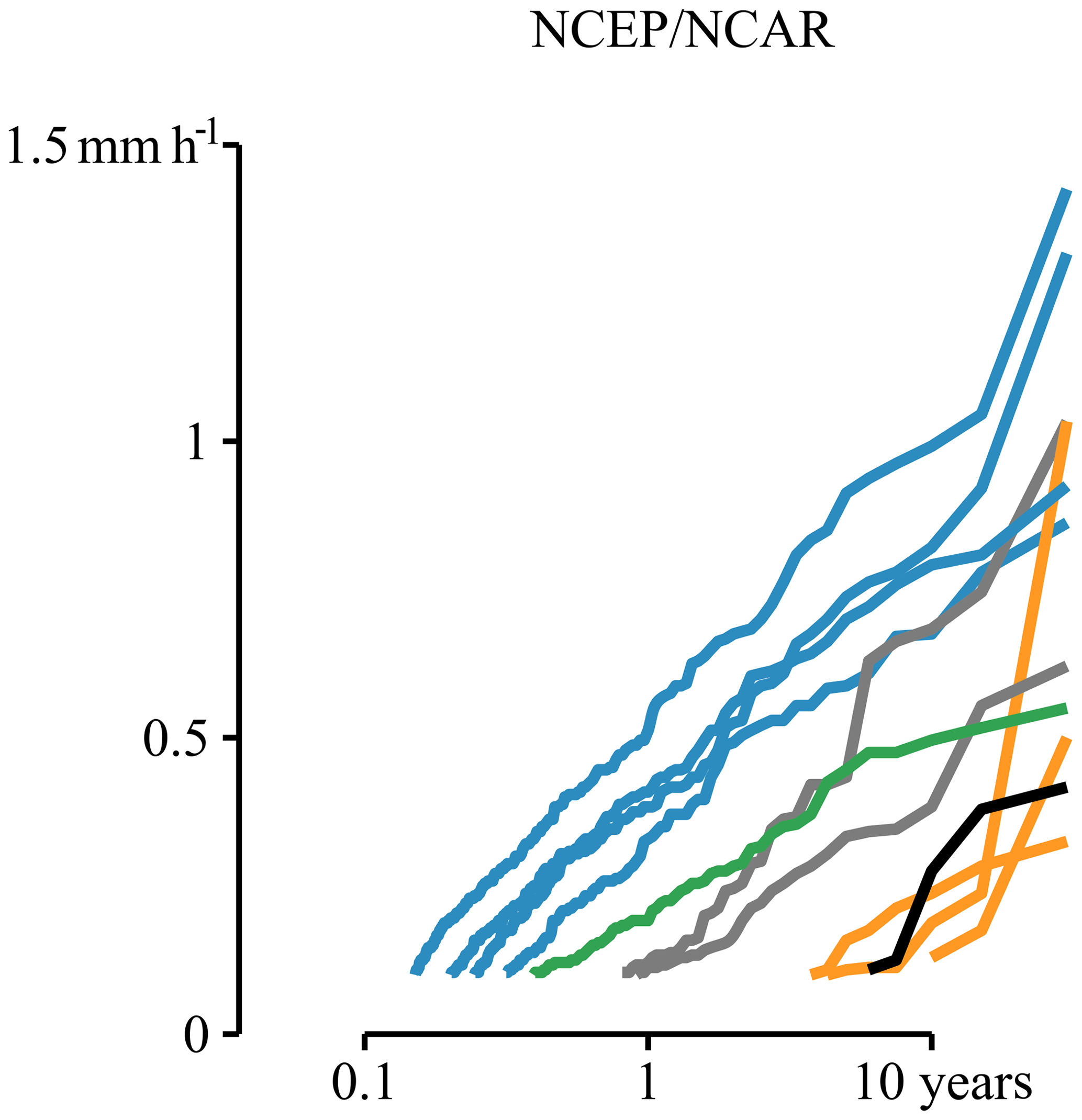
Figure 3Daily winter precipitation amounts per weather type for the NCEP/NCAR reanalysis data set. The blue lines indicate the results for the W, NW, SW, and C WTs, the green line for the A WT, the grey lines for the N and S WTs, the orange lines for the NE, E, SE WTs, and the black line for the U WTs. The results are obtained for the reference period 1961–1990.
The relationship between precipitation and temperature is presented in Fig. 4. This figure demonstrates the intensification of the independent precipitation amounts with increasing temperature. For instance, the 90th percentile precipitation amount increases by 7 % (1 ∘C)−1, and this increase follows the CC relationship. For temperatures higher than 10 ∘C, the scaling rate increases up to 14 % (1 ∘C)−1. Similar scaling rates are obtained for the higher precipitation percentiles. For percentiles smaller than 90 %, the scaling rate of 7 % (1 ∘C)−1 is not identified. The identified CC relationship is similar to other studies for Belgium (De Troch, 2016; Van de Vyver et al., 2019) and for neighbouring regions (Lenderink and van Meijgaard, 2008). Although the CC relationship in those other studies has been established by using the dew point temperature, similar scaling rates are obtained. Considering the findings of recent studies, the application of dew point temperature is expected to better estimate the increases in the atmospheric moisture capacity and, thus, the precipitation changes (Van de Vyver et al., 2019; Wasko et al., 2018).
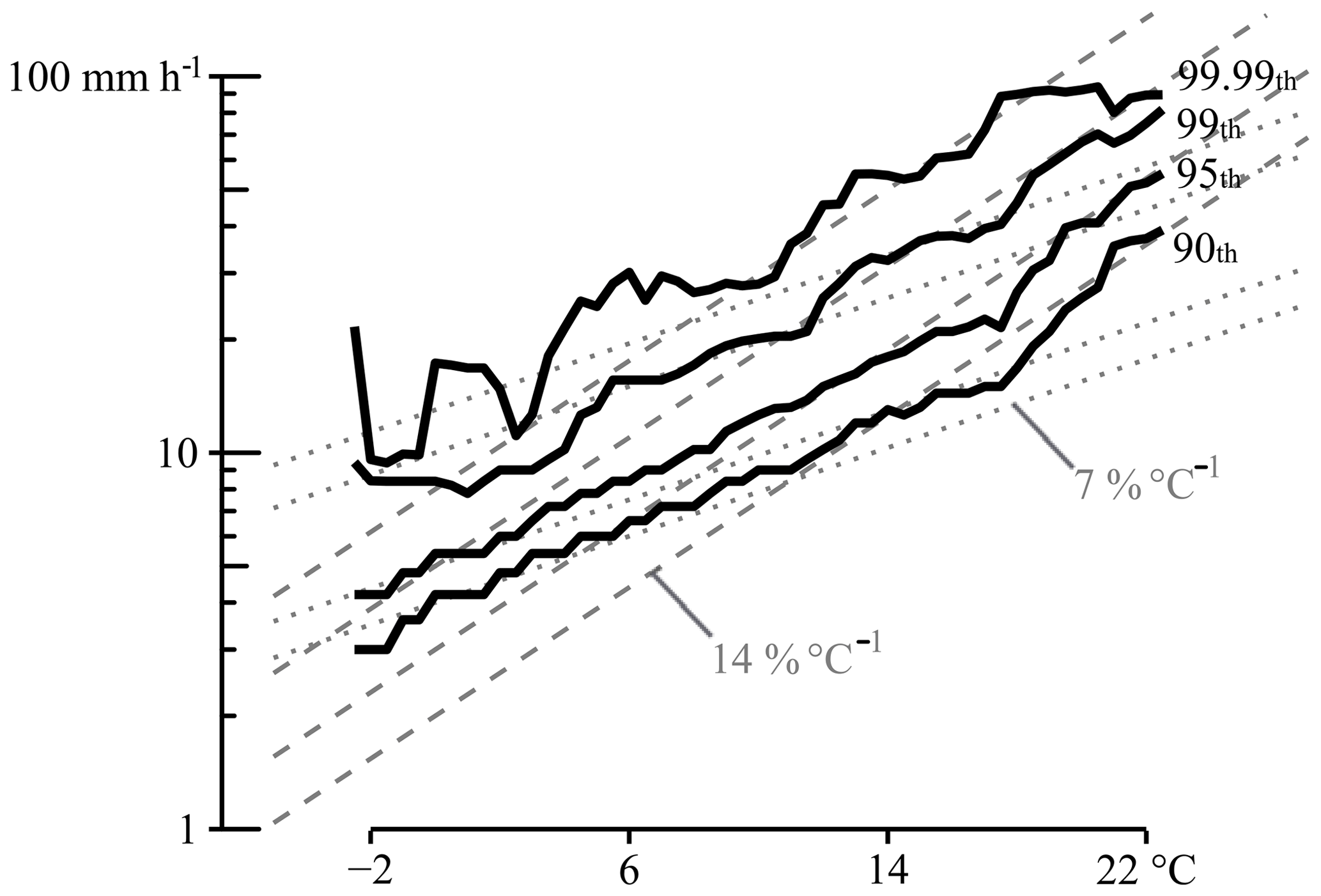
Figure 4The relationship between daily average temperature and independent 10 min precipitation amounts. The relationship is defined by annual timescale, and this is done by using the entire Uccle time series (1901–2000). The CC relationship (+7 % ∘C−1) is indicated by the grey dotted lines, whereas the 2× CC relationship (+14 % ∘C−1) is indicated by the grey dashed lines. The black lines show the magnification of the 90th, 95th, 99th and 99.9th percentile precipitation amount for increasing temperatures.
4.2 The perfect prognosis assumption
Figure 5 compares the WT occurrences for the historical climate model outputs with those for the reanalysis data sets. The comparison reveals large biases, particularly for the W and A WTs. More precisely, the climate models overestimate the occurrence of W WTs by approximately 11 %, whereas the A WTs are underestimated by 14 %. Moreover, in contrast to the reanalysis data sets, the W WTs are the most prominently occurring WTs in the climate model outputs. These findings are in agreement with the recent study by Stryhal and Huth (2018). Using different atmospheric classification patterns, they found an overall overestimation of the westerly circulation, which is estimated to be approximately 7 % for the British Isles and increases towards central Europe by up to 21 %. Otero et al. (2018) and Stryhal and Huth (2018) also indicate that climate models have a poor performance in reproducing the occurrence of A WTs.
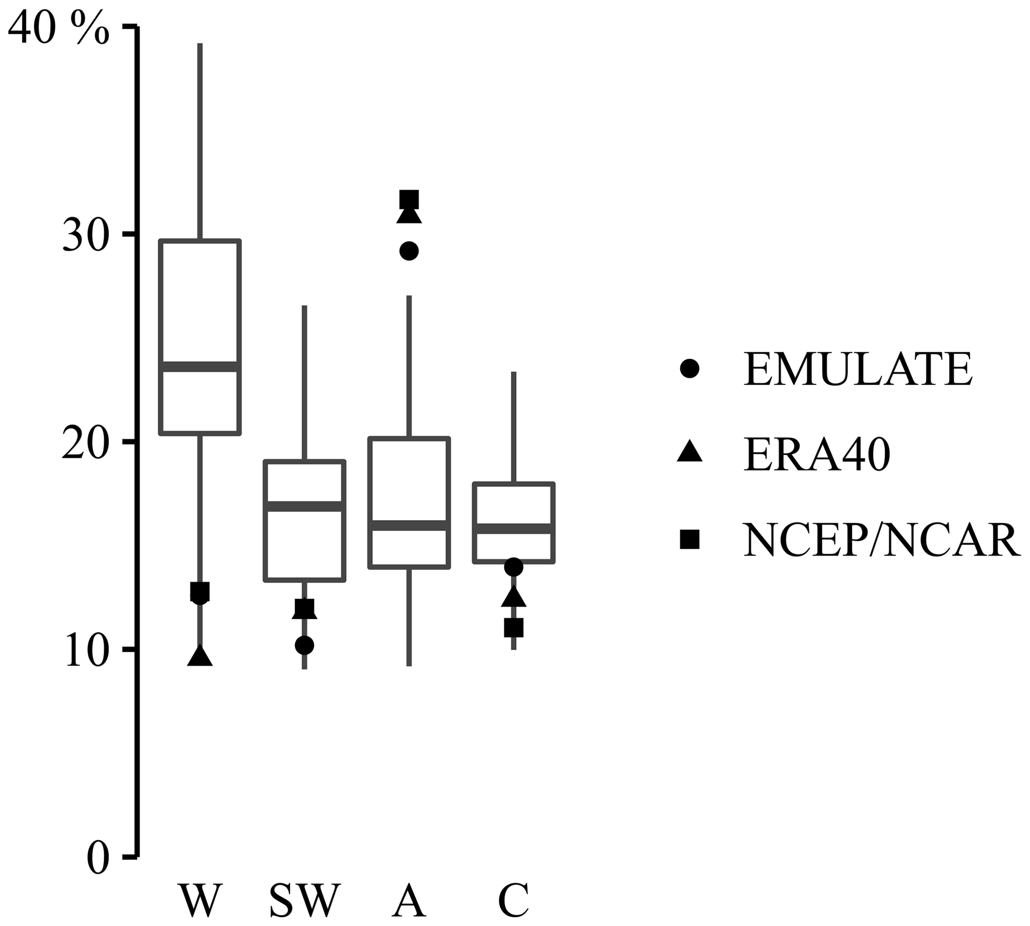
Figure 5Relative WT occurrence in the winter season for different reanalysis data sets (dots) and climate model runs (box plots). The results are obtained for the reference period 1961–1990.
The overestimation of the W WTs is explained by the orientation of the North Atlantic storm track in the climate models. It has, more specifically, a zonal orientation instead of a SW–NE tilt (Pithan et al., 2016; Zappa et al., 2014). The zonal orientation results in a pronounced meridional pressure gradient, creating zonal westerly flows, which in turn impede the occurrences of anticyclones (Stryhal and Huth, 2019). Biases in the blocking frequency are also arising from the climate model resolution (Anstey et al., 2013; Scaife et al., 2011; Woollings et al., 2018).
Although it would be possible to remove the bias in WT occurrences, for instance through resampling (Mehrotra and Sharma, 2019), the studied WT method does not do that. Note that such bias correction would require a technique that simultaneously accounts for the bias in the WT occurrences, the WT persistence, and the relationship between the WTs and other hydrometeorological variables.
4.3 The stationarity assumption
The contribution of the dynamical processes to the precipitation amount changes for the surrogate climate model runs is presented in Fig. 6. Based on the median results, the dynamical processes are responsible for 35 % to 55 % of the changes. The high contributions are most likely explained by the findings of Ntegeka and Willems (2008) and Willems (2013a). These authors identified multidecadal oscillations in the 100-year precipitation time series for Uccle. Some periods are characterised by higher precipitation amounts and are referred to as positive anomalies. The periods characterised by smaller precipitation amounts are referred to as negative anomalies. Willems (2013a) observed that the precipitation anomalies coincide with anomalies in the number of W WTs and with anomalies in the pressure difference between the Azores and Scandinavia. The coincidence of large-scale atmospheric circulation patterns and precipitation amounts has also been studied for other locations in Europe. In this context, Tabari and Willems (2018) identified the North Atlantic Oscillation (NAO) and the El Niño–Southern Oscillation (ENSO) signal as dominant drivers for the extreme winter precipitation amounts. Hence, the findings of Tabari and Willems (2018) and Willems (2013a) imply that large-scale atmospheric circulation influences winter precipitation in Europe. At the end of the 20th century, the dynamical processes explained only 20 % of the precipitation amount changes. This lower contribution is compensated for by a higher contribution from the thermodynamic processes. More specifically, Ntegeka and Willems (2008) point out that the higher precipitation amounts are governed by an intensification of the positive anomaly. The intensification arises from the increasing temperatures, which are in turn attributed to climatic changes.
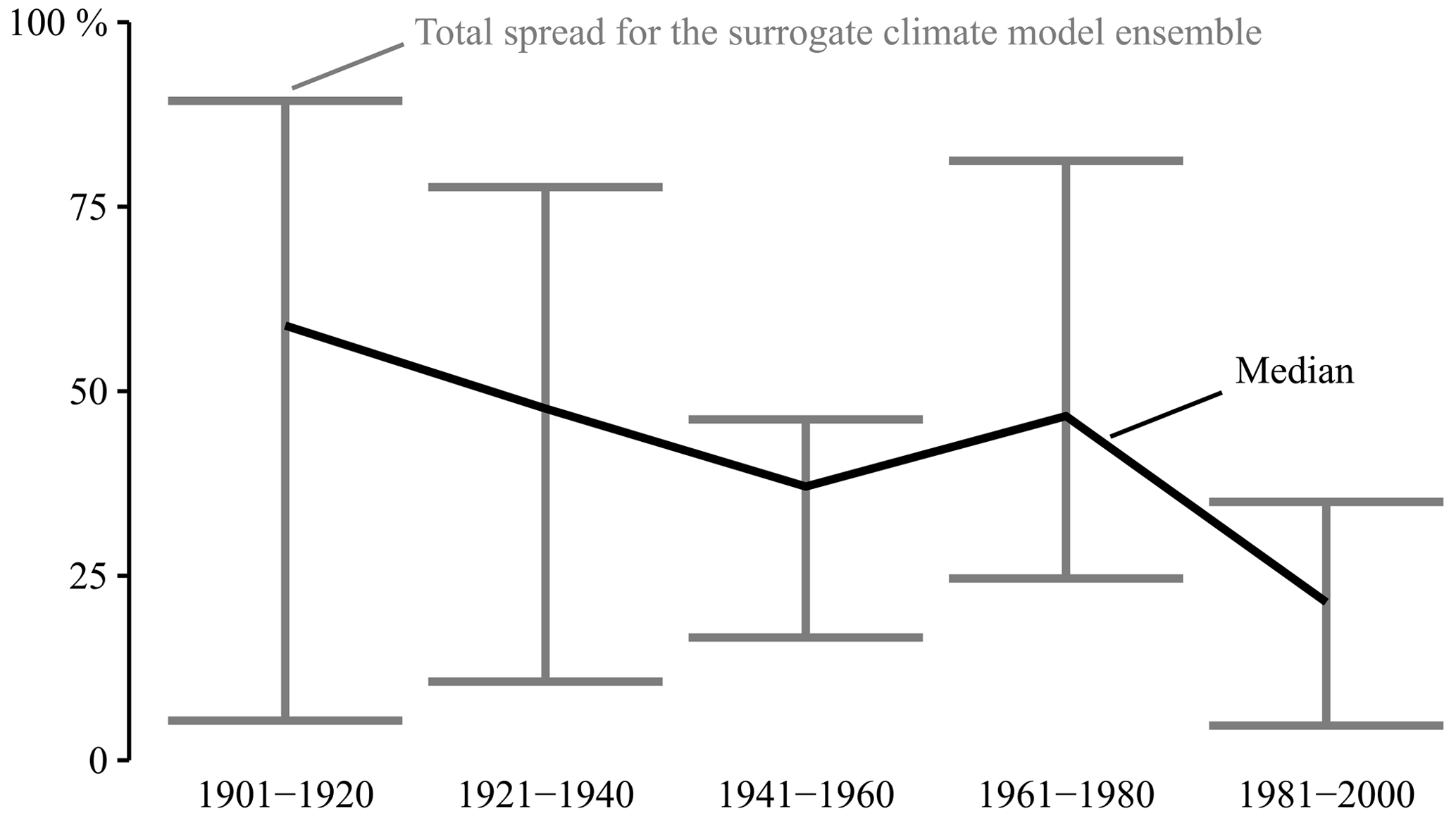
Figure 6Contribution of the dynamical processes to the change in the average precipitation amount of wet days in the function of the choice of the scenario period.
Figure 7 shows the contributions by the dynamical and the thermodynamical processes to the long-term projected changes. The changes in the WTs account for 18 % of the total change and, hence, they are primarily driven by the thermodynamic processes. This is in agreement with the findings of Kröner (2016), who investigated the drivers for precipitation changes in Europe. As the thermodynamic processes are only included to some extent in the downscaling methodology, the applicability of the SDM is questioned. Note that the application of the CC relationship is limited to the extreme precipitation amounts, while the thermodynamic processes also influence the average precipitation amounts.
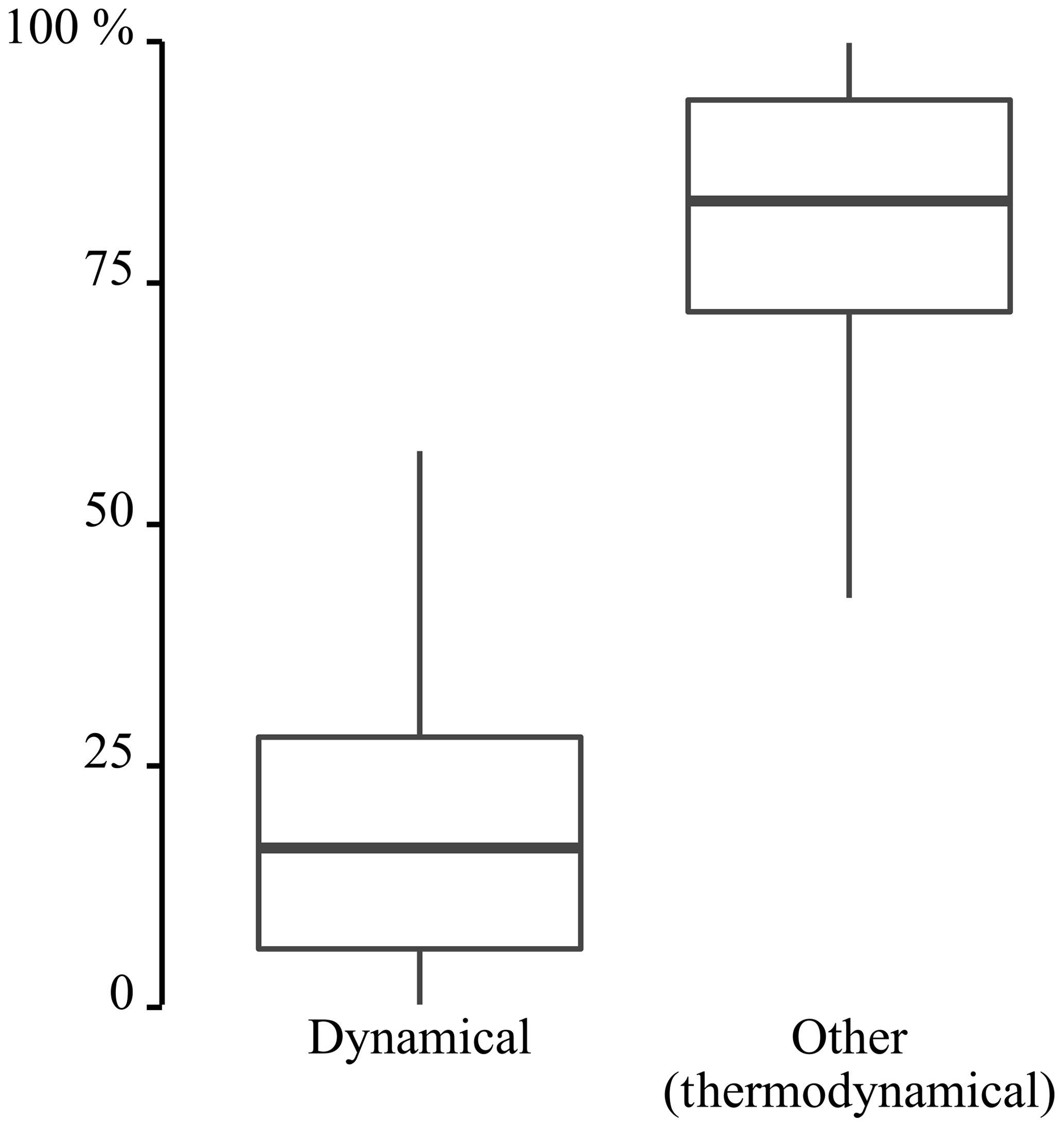
Figure 7Contribution of the dynamical processes, i.e. changes in the WT occurrence frequencies and other effects, for instance, due to the thermodynamic processes, to the change in the average daily precipitation amount of wet winter days. The results are based on the climate model output for the scenario (2071–2100) and control period (1961–1990).
4.4 Response to the greenhouse gas scenarios and the added value of the CC relationship
Climate models project a poleward shift of the Northern Hemisphere jet streams and storm tracks, resulting in the increased occurrence of zonal flows and fewer blocking occurrences (Barnes and Screen, 2015; Santos et al., 2016; Stryhal and Huth, 2019; Woollings et al., 2018). As a consequence, an increasing occurrence of W and SW WTs and a decreasing occurrence of A WTs are projected (Appendix, Fig. A3). More specifically, under the total uncertainty range, i.e. all RCPs combined, the occurrence of W WTs is projected to increase by 7 %. For the RCP sub-ensembles, the increase in W WTs is magnified from 6 % for RCP 4.5 to 11 % for RCP 8.5. The A WTs, on the contrary, decrease in 10 % for RCP 4.5 and 12 % for RCP 8.5. Using the same climate model ensemble, the median change in the average temperature is estimated at 1.6 ∘C for RCP 2.6, 2.1 ∘C for RCP 4.5, 2.6 ∘C for RCP 6.0, and 3.7 ∘C for RCP 8.5 (Termonia et al., 2018).
The changes in the 30-year daily winter precipitation amounts are shown in Fig. 8. While the studied SDM without CC scaling does not project any changes in the 30-year daily precipitation amount, the coarse global climate model (GCM) projections do. This indicates that the reliance of the projections on analogues involves significant shortcomings. Those shortcomings can, however, be overcome by the application of the CC relationship. As a result, an intensification of the extreme precipitation amounts is obtained for the studied SDM. The intensification is, moreover, in agreement with the theoretical estimations. The projected changes for RCP 8.5 are, for instance, estimated at 25.8 % and equal the theoretical change values (3.7 ∘C × 7 %). Note that the CC relationship is applied at the daily timescale and that at the daily timescale the super CC scaling rate (14 % (1 ∘C)−1) is not observed. To some extent, the estimated median change values for the studied SDM differ from the coarse climate model projections. More specifically, the differences in the median change values range between 3 % and 5 %. Besides differences in the change values, there are differences in the monotonicity of the change intensification for increasing greenhouse gas scenarios (GHSs). For the statistically downscaled changes, the intensification of the change values is monotonic due the monotonic increase in the temperature predictor. For the coarse global climate model changes, on the contrary, the monotonicity is masked by random uncertainties, climate model uncertainties and the stochastic uncertainty arising from the internal variability of the climate system (Van Uytven and Willems, 2018).
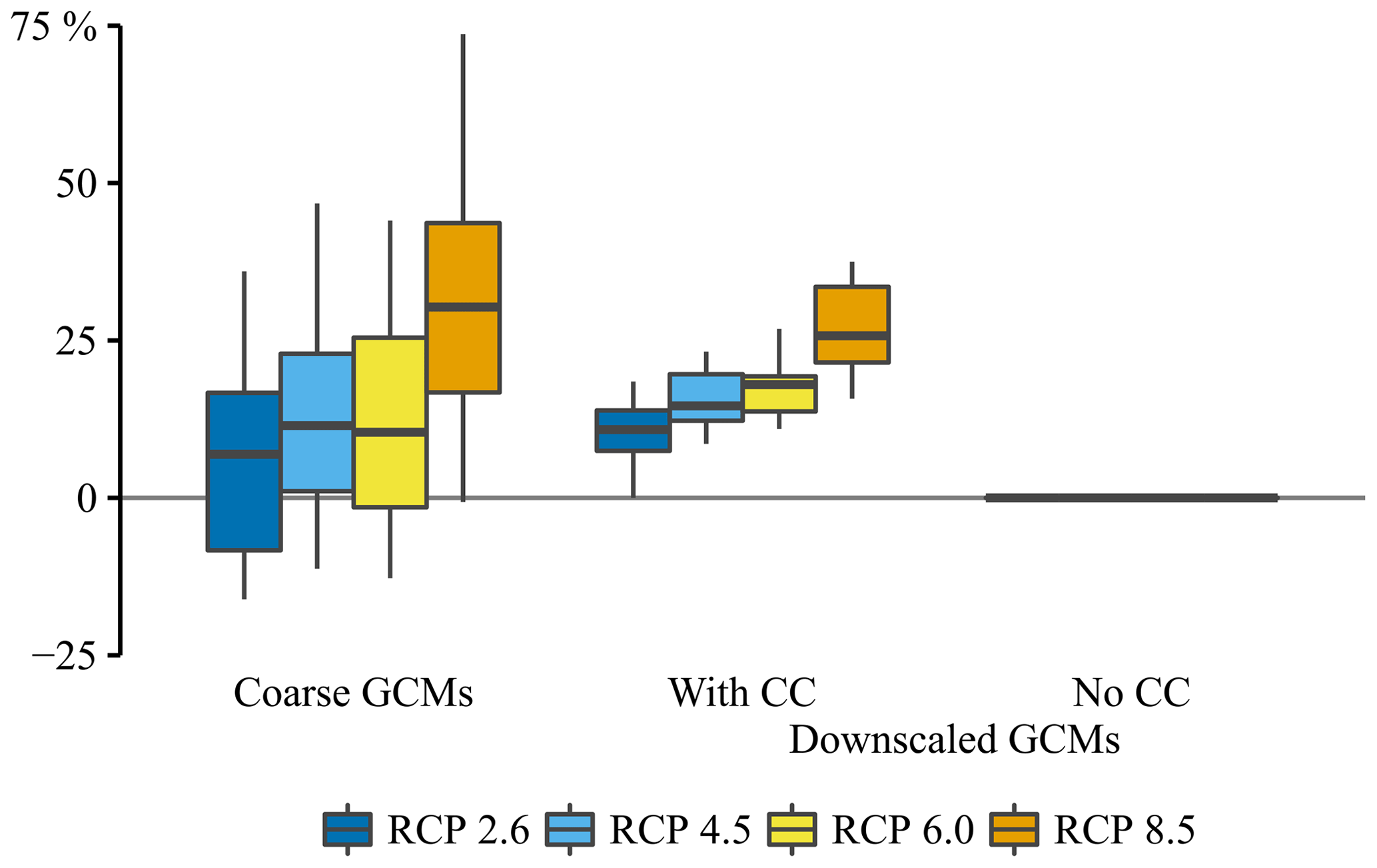
Figure 8Changes in the 30-year daily precipitation winter amount in the function of the different RCPs. The changes are obtained by using the climate model output for 2071–2100 with respect to the output for 1961–1990.
The changes in average winter precipitation accumulation are shown in Fig. 9. The comparison between the coarse climate model changes and the statistically downscaled changes indicates that the statistical downscaling step increases the changes. More specifically, under the total uncertainty range, the statistically downscaled changes are approximately 15 % larger. The latter is explained by the absence of bias correction schemes, the overestimation of the W WTs (Fig. 5), which have been identified as one of the wetter WTs (Sect. 4.1), and the projected increase in these WTs (Fig. A3). Figure 9 furthermore shows that the statistically downscaled changes for the winter precipitation accumulation are not monotonic for increasing greenhouse gas scenarios. The latter is due to the applicability of the CC relationship to extreme precipitation only. For that reason, the monotonicity of the temperature changes is not transferred to the changes in the average winter precipitation accumulation.
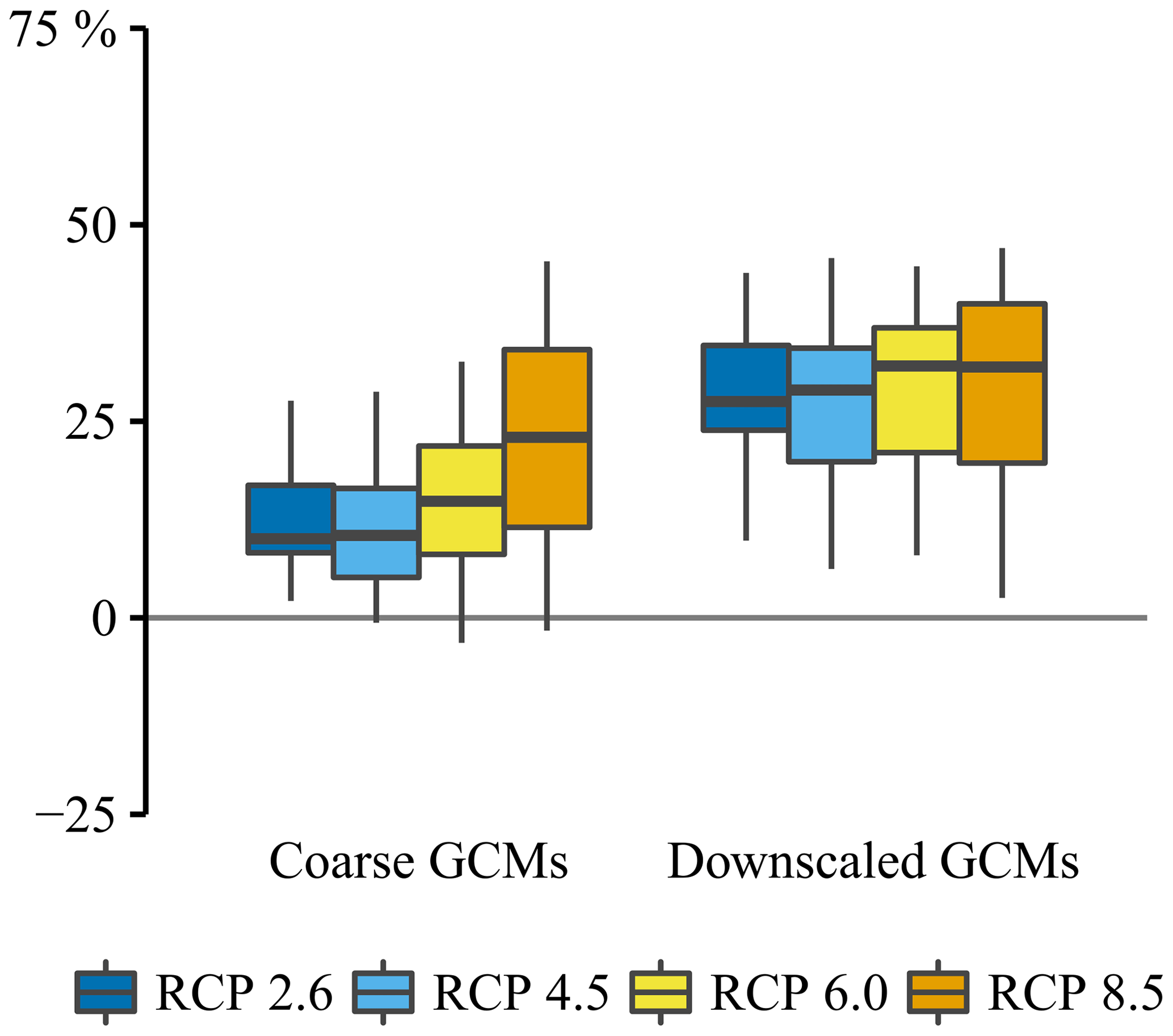
Figure 9Changes in the average winter precipitation accumulation in function of the different RCPs. The changes are obtained by using the climate model output for 2071–2100 with respect to the output for 1961–1990.
The studied SDM does not meet all assumptions. It is shown that the SDM has limitations and its skill could be improved. The WT method fails, among other assumptions, the perfect prognosis assumption. As the method is applied in a perfect prognosis context, improvements should involve the bias correction of the WT occurrences. Since the simulation of large-scale atmospheric circulation patterns remains biased in RCMs (Addor et al., 2016; Jury et al., 2018), the application of a statistical bias correction method is suggested. A potential method would be the recently developed resampling approach of Mehrotra and Sharma (2019). Further extensions to the latter approach are, however, required to also address the biases in the WT persistence and the biases in the relationship between WTs and other hydrometeorological variables. Although the implementation of bias correction methods is possible, it remains questionable whether the WT method may lead to accurate precipitation downscaling. The observations in this study confirm an informative relationship between the predictors and the predictand, but this relationship is time-variant. The WT occurrences explain between 35 % and 55 % of the historical precipitation amount changes, but their contribution decreases to less than 20 % at the end of the 21st century. This means that the precipitation changes for the case study location are controlled by thermodynamic processes rather than dynamical processes (i.e. changes in WT occurrences). As the extreme precipitation amounts are scaled following the CC relationship, the thermodynamic processes are accounted for to some extent in the downscaling methodology but it is not done sufficiently. The CC relationship produces extreme precipitation amounts outside the range of historical observations and thus anticipates the intensification of extreme events. The latter indicates the potential of the CC relationship for improving non-parametric precipitation models. The stand-alone application of the CC relationship as an SDM has recently been demonstrated by Manola et al. (2018) and Van de Vyver et al. (2019), but those SDMs also involve shortcomings (Zhang et al., 2017).
Uncovering the shortcomings of SDMs does not mean that their use is discouraged. One should not forget that other SDMs may also fail assumptions and, thus, also have shortcomings. By considering an ensemble of SDMs, the uncertainties introduced by those shortcomings can be taken into account. When SDM ensembles are considered, ensemble members could be weighted based on their skill. The latter would be similar to the existing climate model weighing techniques (Sanderson et al., 2017). The first step towards a weighted SDM ensemble is still to be made by the statistical downscaling community.
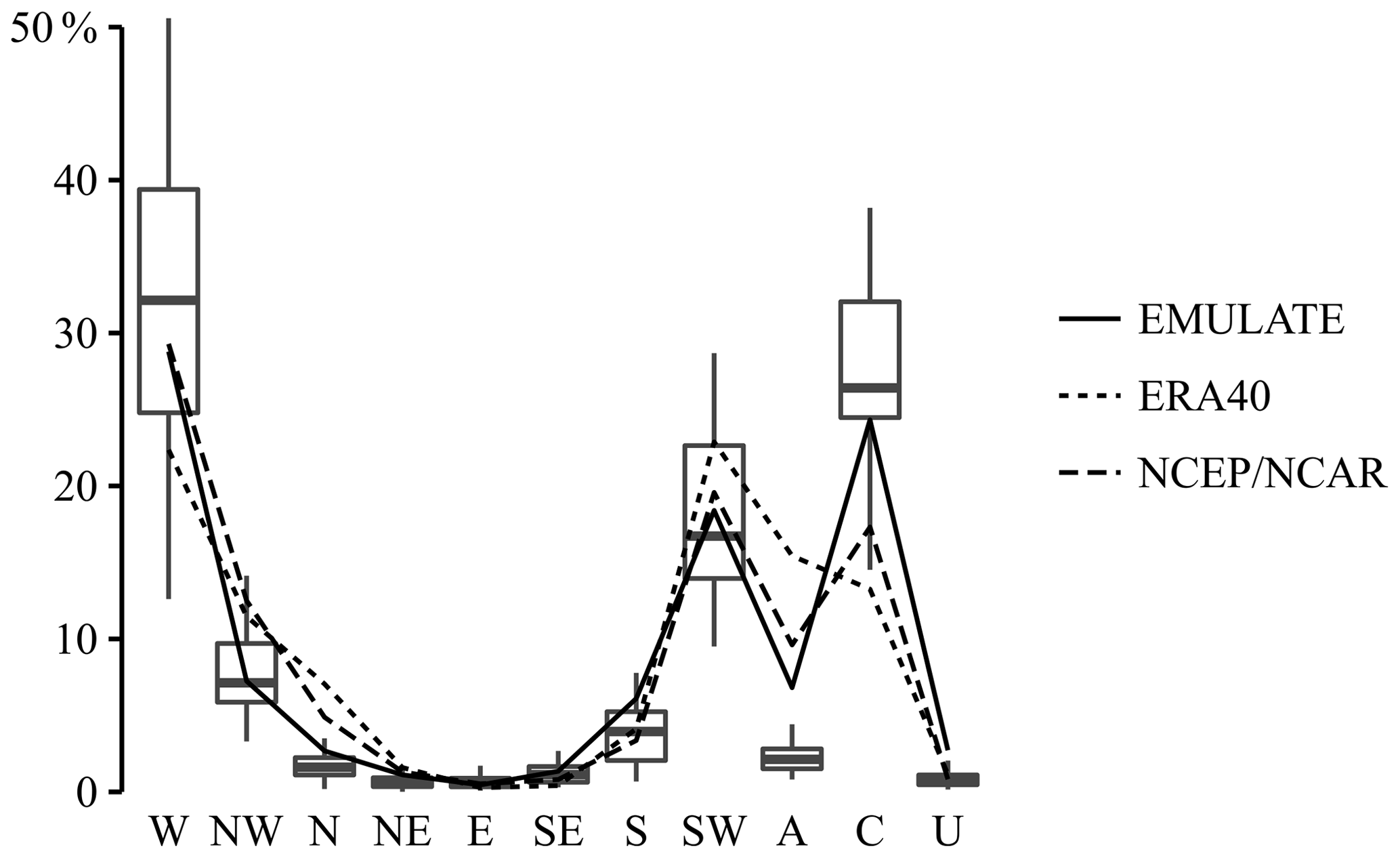
Figure A1Relative winter precipitation accumulation per WT for different reanalysis data sets (lines) and climate model runs (box plots). The results are obtained for the reference period 1961–1990.
Figure A2Percentage of wet days per WT in the winter season for different reanalysis data sets (lines) and climate model runs (box plots). The results are obtained for the reference period 1961–1990.
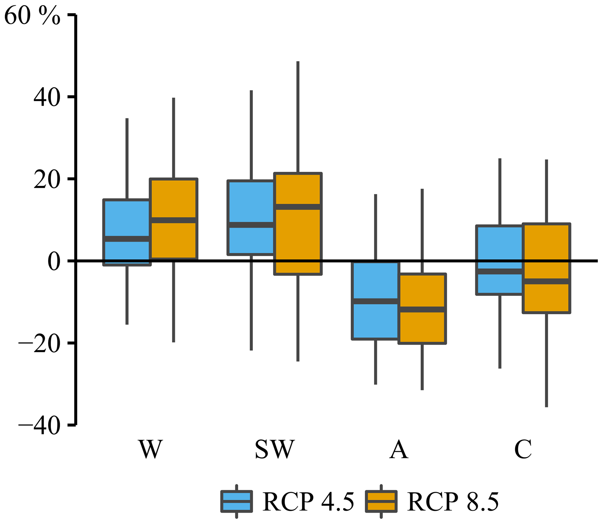
Figure A3Changes in the winter WT occurrences for RCP 4.5 and RCP 8.5. The changes are obtained by using the climate model outputs for 2071–2100 with respect to the output for 1961–1990.
The climate model data are available through the website of the Earth System Grid Federation, https://esgf.llnl.gov/ (Taylor et al., 2012). The ERA40 reanalysis data set is available through the ECMWF Public Datasets Web Interface http://apps.ecmwf.int/datasets/ (Uppala et al., 2005), the EMULATE data set through https://www.metoffice.gov.uk/hadobs/emslp/ (Ansell et al., 2006) and the NCEP/NCAR data set through https://psl.noaa.gov/data/gridded/data.ncep.reanalysis.html (Kalnay et al., 1996). The observed precipitation time series for the Uccle station were made available by the Royal Meteorological Institute of Belgium (KMI).
EVU conceptualised and developed the approaches. Under the supervision of PW, EVU and JDN performed the formal analysis and investigation. EVU prepared the visualisation and wrote the initial draft, which was critically reviewed and revised by PW and JDN.
The authors declare that they have no conflict of interest.
We acknowledge the World Climate Research Programme's (WCRP) Working Group on Coupled Modelling (WGCM), which is responsible for the Coupled Model Intercomparison Project (CMIP), and we thank the climate modelling groups (listed in Table 2) for producing and making their model output available. Els Van Uytven is funded by a doctoral grant from the Research Foundation Flanders (FWO) for her PhD entitled “Evaluation of statistical downscaling methods for climate change impact analysis on hydrological extremes” (FWO, grant no. 11ZY418N). This financial support is gratefully acknowledged.
This research has been supported by the Research Foundation Flanders (FWO grant no. 11ZY418N).
This paper was edited by Shraddhanand Shukla and reviewed by three anonymous referees.
Addor, N., Rohrer, M., Furrer, R., and Seibert, J.: Propagation of biases in climate models from the synoptic to the regional scale: Implications for bias adjustment, J. Geophys. Res.-Atmos., 121, 2075–2089, https://doi.org/10.1002/2015JD024040, 2016. a
Alfieri, L., Feyen, L., and Di Baldassarre, G.: Increasing flood risk under climate change: a pan-European assessment of the benefits of four adaptation strategies, Climatic Change, 136, 507–521, https://doi.org/10.1007/s10584-016-1641-1, 2016. a
Ansell, T. J., Jones, P. D., Allan, R. J., Lister, D., Parker, D. E., Brunet, M., Moberg, A., Jacobeit, J., Brohan, P., Rayner, N. A., Aguilar, E., Alexandersson, H., Barriendos, M., Brandsma, T., Cox, N. J., Della-Marta, P. M., Drebs, A., Founda, D., Gerstengarbe, F., Hickey, K., Jónsson, T., Luterbacher, J., Nordli, Ø., Oesterle, H., Petrakis, M., Philipp, A., Rodwell, M. J., Saladie, O., Sigro, J., Slonosky, V., Srnec, L., Swail, V., García-Suárez, A. M., Tuomenvirta, H., Wang, X., Wanner, H., Werner, P., Wheeler, D., and Xoplaki, E.: Daily mean sea level pressure reconstructions for the European-North Atlantic region for the period 1850–2003, J. Climate, 19, 2717–2742, https://doi.org/10.1175/JCLI3775.1, 2006 (data available at: https://www.metoffice.gov.uk/hadobs/emslp/, last access: 10 May 2020). a, b
Anstey, J. A., Davini, P., Gray, L. J., Woollings, T. J., Butchart, N., Cagnazzo, C., Christiansen, B., Hardiman, S. C., Osprey, S. M., and Yang, S.: Multi-model analysis of Northern Hemisphere winter blocking: Model biases and the role of resolution, J. Geophys. Res.-Atmos., 118, 3956–3971, https://doi.org/10.1002/jgrd.50231, 2013. a, b
Arakawa, A.: The Cumulus Parameterization Problem: Past, Present, and Future, J. Climate, 17, 2493–2525, https://doi.org/10.1175/1520-0442(2004)017<2493:RATCPP>2.0.CO;2, 2004. a
Åström, H. L., Sunyer, M., Madsen, H., Rosbjerg, D., and Arnbjerg-Nielsen, K.: Explanatory analysis of the relationship between atmospheric circulation and occurrence of flood-generating events in a coastal city, Hydrol. Process., 30, 2773–2788, https://doi.org/10.1002/hyp.10767, 2016. a, b
Barbero, R., Westra, S., Lenderink, G., and Fowler, H. J.: Temperature-extreme precipitation scaling: a two-way causality?, Int. J. Climatol., 38, e1274–e1279, https://doi.org/10.1002/joc.5370, 2018. a
Barnes, E. A. and Screen, J. A.: The impact of Arctic warming on the midlatitude jet-stream: Can it? Has it? Will it?, WIRES: Climate Change, 6, 277–286, https://doi.org/10.1002/wcc.337, 2015. a
Benestad, R. E., Hanssen-Bauer, I., and Chen, D.: Empirical-Statistical Downscaling, WORLD SCIENTIFIC, https://doi.org/10.1142/6908, 2008. a
Blenkinsop, S., Fowler, H. J., Barbero, R., Chan, S. C., Guerreiro, S. B., Kendon, E., Lenderink, G., Lewis, E., Li, X.-F., Westra, S., Alexander, L., Allan, R. P., Berg, P., Dunn, R. J. H., Ekström, M., Evans, J. P., Holland, G., Jones, R., Kjellström, E., Klein-Tank, A., Lettenmaier, D., Mishra, V., Prein, A. F., Sheffield, J., and Tye, M. R.: The INTENSE project: using observations and models to understand the past, present and future of sub-daily rainfall extremes, Adv. Sci. Res., 15, 117–126, https://doi.org/10.5194/asr-15-117-2018, 2018. a
Brekke, L. D., Maurer, E. P., Anderson, J. D., Dettinger, M. D., Townsley, E. S., Harrison, A., and Pruitt, T.: Assessing reservoir operations risk under climate change, Water Resour. Res., 45, 1–16, https://doi.org/10.1029/2008WR006941, 2009. a
Brisson, E., Demuzere, M., Kwakernaak, B., and Van Lipzig, N. P.: Relations between atmospheric circulation and precipitation in Belgium, Meteorol. Atmos. Phys., 111, 27–39, https://doi.org/10.1007/s00703-010-0103-y, 2011. a
Bürger, G., Murdock, T. Q., Werner, A. T., Sobie, S. R., and Cannon, A. J.: Downscaling Extremes – An Intercomparison of Multiple Statistical Methods for Present Climate, J. Climate, 25, 4366–4388, https://doi.org/10.1175/JCLI-D-11-00408.1, 2012. a
Casanueva, A., Herrera, S., Fernández, J., and Gutiérrez, J. M.: Towards a fair comparison of statistical and dynamical downscaling in the framework of the EURO-CORDEX initiative, Climatic Change, 137, 411–426, https://doi.org/10.1007/s10584-016-1683-4, 2016. a
Cristiano, E., ten Veldhuis, M.-C., Gaitan, S., Ochoa Rodriguez, S., and van de Giesen, N.: Critical scales to explain urban hydrological response: an application in Cranbrook, London, Hydrol. Earth Syst. Sci., 22, 2425–2447, https://doi.org/10.5194/hess-22-2425-2018, 2018. a
Davini, P., Corti, S., D'Andrea, F., Rivière, G., and von Hardenberg, J.: Improved Winter European Atmospheric Blocking Frequencies in High-Resolution Global Climate Simulations, J. Adv. Model. Earth Syst., 9, 2615–2634, https://doi.org/10.1002/2017MS001082, 2017. a
Demuzere, M., Werner, M., van Lipzig, N. P. M., and Roeckner, E.: An analysis of present and future ECHAM5 pressure fields using a classification of circulation patterns, Int. J. Climatol., 29, 1796–1810, https://doi.org/10.1002/joc.1821, 2009. a
De Niel, J., Demarée, G., and Willems, P.: Weather Typing-Based Flood Frequency Analysis Verified for Exceptional Historical Events of Past 500 Years Along the Meuse River, Water Resour. Res., 53, 8459–8474, https://doi.org/10.1002/2017WR020803, 2017. a
Deser, C., Phillips, A., Bourdette, V., and Teng, H.: Uncertainty in climate change projections: The role of internal variability, Clim. Dynam., 38, 527–546, https://doi.org/10.1007/s00382-010-0977-x, 2012. a
De Troch, R.: The application of the ALARO-0 model for regional climate modeling in Belgium: extreme precipitation and unfavorable conditions for the dispersion of air pollutants under present and future climate conditions, available at: https://biblio.ugent.be/publication/7247081 (last access: 10 May 2020), 2016. a
Dixon, K. W., Lanzante, J. R., Nath, M. J., Hayhoe, K., Stoner, A., Radhakrishnan, A., Balaji, V., and Gaitán, C. F.: Evaluating the stationarity assumption in statistically downscaled climate projections: is past performance an indicator of future results?, Climatic Change, 135, 395–408, https://doi.org/10.1007/s10584-016-1598-0, 2016. a, b
Dottori, F., Szewczyk, W., Ciscar, J.-C., Zhao, F., Alfieri, L., Hirabayashi, Y., Bianchi, A., Mongelli, I., Frieler, K., Betts, R., and Feyen, L.: Increased human and economic losses from river flooding with anthropogenic warming, Nat. Clim. Change, 8, 781–786, https://doi.org/10.1038/s41558-018-0257-z, 2018. a
Ehret, U., Zehe, E., Wulfmeyer, V., Warrach-Sagi, K., and Liebert, J.: HESS Opinions “Should we apply bias correction to global and regional climate model data?”, Hydrol. Earth Syst. Sci., 16, 3391–3404, https://doi.org/10.5194/hess-16-3391-2012, 2012. a
Emori, S. and Brown, S. J.: Dynamic and thermodynamic changes in mean and extreme precipitation under changed climate, Geophys. Res. Lett., 32, 1–5, https://doi.org/10.1029/2005GL023272, 2005. a
Fadhel, S., Rico-Ramirez, M. A., and Han, D.: Uncertainty of Intensity–Duration–Frequency (IDF) curves due to varied climate baseline periods, J. Hydrol., 547, 600–612, https://doi.org/10.1016/j.jhydrol.2017.02.013, 2017. a
Flaounas, E., Drobinski, P., Vrac, M., Bastin, S., Lebeaupin-Brossier, C., Stéfanon, M., Borga, M., and Calvet, J. C.: Precipitation and temperature space-time variability and extremes in the Mediterranean region: Evaluation of dynamical and statistical downscaling methods, Clim. Dynam., 40, 2687–2705, https://doi.org/10.1007/s00382-012-1558-y, 2013. a
Fu, G., Charles, S. P., Chiew, F. H., Ekström, M., and Potter, N. J.: Uncertainties of statistical downscaling from predictor selection: Equifinality and transferability, Atmos. Res., 203, 130–140, https://doi.org/10.1016/j.atmosres.2017.12.008, 2018. a, b
Gutmann, E., Pruitt, T., Clark, M. P., Brekke, L., Arnold, J. R., Raff, D. A., and Rasmussen, R. M.: An intercomparison of statistical downscaling methods used for water resource assessments in the United States, Water Resour. Res., 50, 7167–7186, https://doi.org/10.1002/2014WR015559, 2014. a
Haberlandt, U., Belli, A., and Bárdossy, A.: Statistical downscaling of precipitation using a stochastic rainfall model conditioned on circulation patterns – an evaluation of assumptions, Int. J. Climatol., 35, 417–432, https://doi.org/10.1002/joc.3989, 2015. a
Hartung, K., Svensson, G., and Kjellström, E.: Resolution, physics and atmosphere–ocean interaction – How do they influence climate model representation of Euro-Atlantic atmospheric blocking?, Tellus A, 69, 1406252, https://doi.org/10.1080/16000870.2017.1406252, 2017. a
Hertig, E., Merkenschlager, C., and Jacobeit, J.: Change points in predictors–predictand relationships within the scope of statistical downscaling, Int. J. Climatol., 37, 1619–1633, https://doi.org/10.1002/joc.4801, 2017. a
Hertig, E., Maraun, D., Bartholy, J., Pongracz, R., Vrac, M., Mares, I., Gutiérrez, J. M., Wibig, J., Casanueva, A., and Soares, P. M. M.: Comparison of statistical downscaling methods with respect to extreme events over Europe: Validation results from the perfect predictor experiment of the COST Action VALUE, Int. J. Climatol., 39, 3846–3867, https://doi.org/10.1002/joc.5469, 2018. a
Hewitson, B. C., Daron, J., Crane, R. G., Zermoglio, M. F., and Jack, C.: Interrogating empirical-statistical downscaling, Climatic Change, 122, 539–554, https://doi.org/10.1007/s10584-013-1021-z, 2014. a
Horton, P. and Brönnimann, S.: Impact of global atmospheric reanalyses on statistical precipitation downscaling, Clim. Dynam., 52, 5189–5211, https://doi.org/10.1007/s00382-018-4442-6, 2018. a
Jenkinson, A. and Collison, F.: An initial climatology of gales over the North Sea, Synoptic Climatology Branch Memorandum, Meteorological Office, Bracknell, UK, 62, 1977. a
Jones, P. D., Hulme, M., and Briffa, K. R.: A comparison of Lamb circulation types with an objective classification scheme, Int. J. Climatol., 13, 655–663, https://doi.org/10.1002/joc.3370130606, 1993. a
Jury, M. W., Herrera, S., Gutiérrez, J. M., and Barriopedro, D.: Blocking representation in the ERA-Interim driven EURO-CORDEX RCMs, Clim. Dynam., 52, 3291–3306, https://doi.org/10.1007/s00382-018-4335-8, 2018. a
Kalnay, E., Kanamitsu, M., Kistler, R., Collins, W., Deaven, D., Gandin, L., Iredell, M., Saha, S., White, G., Woollen, J., Zhu, Y., Chelliah, M., Ebisuzaki, W., Higgins, W., Janowiak, J., Mo, K. C., Ropelewski, C., Wang, J., Leetmaa, A., Reynolds, R., Jenne, R., and Joseph, D.: The NCEP/NCAR 40-Year Reanalysis Project, B. Am. Meteorol. Soc., 77, 437–472, https://doi.org/10.1175/1520-0477(1996)077<0437:TNYRP>2.0.CO;2, 1996 (data available at: https://psl.noaa.gov/data/gridded/data.ncep.reanalysis.html, last access: 10 May 2020). a, b
Kotlarski, S., Keuler, K., Christensen, O. B., Colette, A., Déqué, M., Gobiet, A., Goergen, K., Jacob, D., Lüthi, D., van Meijgaard, E., Nikulin, G., Schär, C., Teichmann, C., Vautard, R., Warrach-Sagi, K., and Wulfmeyer, V.: Regional climate modeling on European scales: a joint standard evaluation of the EURO-CORDEX RCM ensemble, Geosci. Model Dev., 7, 1297–1333, https://doi.org/10.5194/gmd-7-1297-2014, 2014. a
Kröner, N.: Identifying and quantifying large-scale drivers of European climate change, ETH Zürich, https://doi.org/10.3929/ethz-a-010793497, 2016. a
Kröner, N., Kotlarski, S., Fischer, E., Lüthi, D., Zubler, E., and Schär, C.: Separating climate change signals into thermodynamic, lapse-rate and circulation effects: theory and application to the European summer climate, Clim. Dynam., 48, 3425–3440, https://doi.org/10.1007/s00382-016-3276-3, 2017. a
Lanzante, J. R., Dixon, K. W., Nath, M. J., Whitlock, C. E., and Adams-Smith, D.: Some Pitfalls in Statistical Downscaling of Future Climate, B. Am. Meteorol. Soc., 99, 791–803, https://doi.org/10.1175/BAMS-D-17-0046.1, 2018. a
Lenderink, G. and van Meijgaard, E.: Increase in hourly precipitation extremes beyond expectations from temperature changes, Nat. Geosci., 1, 511–514, https://doi.org/10.1038/ngeo262, 2008. a
Lenderink, G., Barbero, R., Loriaux, J. M., and Fowler, H. J.: Super-Clausius-Clapeyron scaling of extreme hourly convective precipitation and its relation to large-scale atmospheric conditions, J. Climate, 30, 6037–6052, https://doi.org/10.1175/JCLI-D-16-0808.1, 2017. a
Le Roux, R., Katurji, M., Zawar-Reza, P., Quénol, H., and Sturman, A.: Comparison of statistical and dynamical downscaling results from the WRF model, Environ. Modell. Softw., 100, 67–73, https://doi.org/10.1016/j.envsoft.2017.11.002, 2018. a
Li, J., Johnson, F., Evans, J., and Sharma, A.: A comparison of methods to estimate future sub-daily design rainfall, Adv. Water Resour., 110, 215–227, https://doi.org/10.1016/j.advwatres.2017.10.020, 2017. a
Manola, I., van den Hurk, B., De Moel, H., and Aerts, J. C. J. H.: Future extreme precipitation intensities based on a historic event, Hydrol. Earth Syst. Sci., 22, 3777–3788, https://doi.org/10.5194/hess-22-3777-2018, 2018. a, b, c
Maraun, D.: Bias Correcting Climate Change Simulations – a Critical Review, Current Climate Change Reports, 2, 211–220, https://doi.org/10.1007/s40641-016-0050-x, 2016. a
Maraun, D. and Widmann, M.: Statistical Downscaling and Bias Correction for Climate Research, Cambridge University Press, https://doi.org/10.1017/9781107588783, 2018. a, b, c
Maraun, D., Wetterhall, F., Chandler, R. E., Kendon, E. J., Widmann, M., Brienen, S., Rust, H. W., Sauter, T., Themeßl, M., Venema, V. K. C., Chun, K. P., Goodess, C. M., Jones, R. G., Onof, C., Vrac, M., and Thiele-Eich, I.: Precipitation downscaling under climate change: Recent developements to bridge the gap between dynamical models and the end user, Rev. Geophys., 48, 1–38, https://doi.org/10.1029/2009RG000314, 2010. a, b, c
Maraun, D., Widmann, M., and Gutiérrez, J. M.: Statistical downscaling skill under present climate conditions: A synthesis of the VALUE perfect predictor experiment, Int. J. Climatol., 39, 3692–3703, https://doi.org/10.1002/joc.5877, 2018. a
Mehrotra, R. and Sharma, A.: A Resampling Approach for Correcting Systematic Spatiotemporal Biases for Multiple Variables in a Changing Climate, Water Resour. Res., 55, 754–770, https://doi.org/10.1029/2018WR023270, 2019. a, b
Mendoza, P. A., Mizukami, N., Ikeda, K., Clark, M. P., Gutmann, E. D., Arnold, J. R., Brekke, L. D., and Rajagopalan, B.: Effects of different regional climate model resolution and forcing scales on projected hydrologic changes, J. Hydrol., 541, 1003–1019, https://doi.org/10.1016/j.jhydrol.2016.08.010, 2016. a
Merkenschlager, C., Hertig, E., and Jacobeit, J.: Non-stationarities in the relationships of heavy precipitation events in the Mediterranean area and the large-scale circulation in the second half of the 20th century, Global Planet. Change, 151, 108–121, https://doi.org/10.1016/j.gloplacha.2016.10.009, 2017. a
Ntegeka, V. and Willems, P.: Trends and multidecadal oscillations in rainfall extremes, based on a more than 100-year time series of 10 min rainfall intensities at Uccle, Belgium, Water Resour. Res., 44, 1–15, https://doi.org/10.1029/2007WR006471, 2008. a, b
Otero, N., Sillmann, J., and Butler, T.: Assessment of an extended version of the Jenkinson–Collison classification on CMIP5 models over Europe, Clim. Dynam., 50, 1559–1579, https://doi.org/10.1007/s00382-017-3705-y, 2018. a, b, c
Philipp, A., Beck, C., Huth, R., and Jacobeit, J.: Development and comparison of circulation type classifications using the COST 733 dataset and software, Int. J. Climatol., 36, 2673–2691, https://doi.org/10.1002/joc.3920, 2016. a
Pithan, F., Shepherd, T. G., Zappa, G., and Sandu, I.: Climate model biases in jet streams, blocking and storm tracks resulting from missing orographic drag, Geophys. Res. Lett., 43, 7231–7240, https://doi.org/10.1002/2016GL069551, 2016. a
Prein, A. F., Langhans, W., Fosser, G., Ferrone, A., Ban, N., Goergen, K., Keller, M., Tölle, M., Gutjahr, O., Feser, F., Brisson, E., Kollet, S., Schmidli, J., Van Lipzig, N. P., and Leung, R.: A review on regional convection-permitting climate modeling: Demonstrations, prospects, and challenges, Rev. Geophys., 53, 323–361, https://doi.org/10.1002/2014RG000475, 2015. a
Roberts, D. R., Wood, W. H., and Marshall, S. J.: Assessments of downscaled climate data with a high-resolution weather station network, Int. J. Climatol., 39, 3091–3103, https://doi.org/10.1002/joc.6005, 2019. a
Rybka, H. and Tost, H.: Uncertainties in future climate predictions due to convection parameterisations, Atmos. Chem. Phys., 14, 5561–5576, https://doi.org/10.5194/acp-14-5561-2014, 2014. a
Sachindra, D. A., Ahmed, K., Shahid, S., and Perera, B. J. C.: Cautionary note on the use of genetic programming in statistical downscaling, Int. J. Climatol., 38, 3449–3465, https://doi.org/10.1002/joc.5508, 2018. a
Salvadore, E., Bronders, J., and Batelaan, O.: Hydrological modelling of urbanized catchments: A review and future directions, J. Hydrol., 529, 62–81, https://doi.org/10.1016/j.jhydrol.2015.06.028, 2015. a
Salvi, K., Ghosh, S., and Ganguly, A. R.: Credibility of statistical downscaling under nonstationary climate, Clim. Dynam., 46, 1991–2023, https://doi.org/10.1007/s00382-015-2688-9, 2016. a, b
Sanderson, B. M., Wehner, M., and Knutti, R.: Skill and independence weighting for multi-model assessments, Geosci. Model Dev., 10, 2379–2395, https://doi.org/10.5194/gmd-10-2379-2017, 2017. a
Santos, J. A., Belo-Pereira, M., Fraga, H., and Pinto, J. G.: Understanding climate change projections for precipitation over western Europe with a weather typing approach, J. Geophys. Res.-Atmos., 121, 1170–1189, https://doi.org/10.1002/2015JD024399, 2016. a, b
Scaife, A. A., Copsey, D., Gordon, C., Harris, C., Hinton, T., Keeley, S., O'Neill, A., Roberts, M., and Williams, K.: Improved Atlantic winter blocking in a climate model, Geophys. Res. Lett., 38, L23703, https://doi.org/10.1029/2011GL049573, 2011. a
Schiemann, R. and Frei, C.: How to quantify the resolution of surface climate by circulation types: An example for Alpine precipitation, Phys. Chem. Earth, 35, 403–410, https://doi.org/10.1016/j.pce.2009.09.005, 2010. a
Schoof, J. T.: Statistical Downscaling in Climatology, Geography Compass, 7, 249–265, https://doi.org/10.1111/gec3.12036, 2013. a, b
Shepherd, T. G., Boyd, E., Calel, R. A., Chapman, S. C., Dessai, S., Dima-West, I. M., Fowler, H. J., James, R., Maraun, D., Martius, O., Senior, C. A., Sobel, A. H., Stainforth, D. A., Tett, S. F. B., Trenberth, K. E., van den Hurk, B. J. J. M., Watkins, N. W., Wilby, R. L., and Zenghelis, D. A.: Storylines: an alternative approach to representing uncertainty in physical aspects of climate change, Climatic Change, 151, 555–571, https://doi.org/10.1007/s10584-018-2317-9, 2018. a
Sørup, H. J. D., Davidsen, S., Löwe, R., Thorndahl, S. L., Borup, M., and Arnbjerg-Nielsen, K.: Evaluating catchment response to artificial rainfall from four weather generators for present and future climate, Water Sci. Technol., 77, 2578–2588, https://doi.org/10.2166/wst.2018.217, 2018. a
Souverijns, N., Thiery, W., Demuzere, M., and Lipzig, N. P. M. V.: Drivers of future changes in East African precipitation Drivers of future changes in East African precipitation, Environ. Res. Lett., 11, 1–9, https://doi.org/10.1088/1748-9326/11/11/114011, 2016. a
Stocker, T., Qin, D., Plattner, G.-K., Tignor, M., Allen, S., Boschung, J., Nauels, A., Xia, Y., Bex, V., and Midgley, P.: Summary for Policymakers, book section SPM, Cambridge University Press, Cambridge, UK and New York, NY, USA, 1–30, https://doi.org/10.1017/CBO9781107415324.004, 2013. a
Stryhal, J. and Huth, R.: Classifications of winter Euro-Atlantic circulation patterns: An intercomparison of five atmospheric reanalyses, J. Climate, 30, 7847–7861, https://doi.org/10.1175/JCLI-D-17-0059.1, 2017. a
Stryhal, J. and Huth, R.: Classifications of winter atmospheric circulation patterns: validation of CMIP5 GCMs over Europe and the North Atlantic, Clim. Dynam., 52, 3575–3598, https://doi.org/10.1007/s00382-018-4344-7, 2018. a, b
Stryhal, J. and Huth, R.: Trends in winter circulation over the British Isles and central Europe in twenty-first century projections by 25 CMIP5 GCMs, Clim. Dynam., 52, 1063–1075, https://doi.org/10.1007/s00382-018-4178-3, 2019. a, b
Sunyer, M. A., Hundecha, Y., Lawrence, D., Madsen, H., Willems, P., Martinkova, M., Vormoor, K., Bürger, G., Hanel, M., Kriaučiūnienė, J., Loukas, A., Osuch, M., and Yücel, I.: Inter-comparison of statistical downscaling methods for projection of extreme precipitation in Europe, Hydrol. Earth Syst. Sci., 19, 1827–1847, https://doi.org/10.5194/hess-19-1827-2015, 2015. a, b
Tabari, H. and Willems, P.: Lagged influence of Atlantic and Pacific climate patterns on European extreme precipitation, Sci. Rep., 8, 5748, https://doi.org/10.1038/s41598-018-24069-9, 2018. a, b
Tabari, H., De Troch, R., Giot, O., Hamdi, R., Termonia, P., Saeed, S., Brisson, E., Van Lipzig, N., and Willems, P.: Local impact analysis of climate change on precipitation extremes: are high-resolution climate models needed for realistic simulations?, Hydrol. Earth Syst. Sci., 20, 3843–3857, https://doi.org/10.5194/hess-20-3843-2016, 2016. a, b, c
Taylor, K. E., Stouffer, R. J., and Meehl, G. A.: An Overview of CMIP5 and the experiment design, B. Am. Meteorol. Soc., 93, 485–498, https://doi.org/10.1175/BAMS-D-11-00094.1, 2012 (data available at: https://esgf.llnl.gov/, last access: 10 May 2020). a
Termonia, P., Van Schaeybroeck, B., De Cruz, L., De Troch, R., Caluwaerts, S., Giot, O., Hamdi, R., Vannitsem, S., Duchêne, F., Willems, P., Tabari, H., Van Uytven, E., Hosseinzadehtalaei, P., Van Lipzig, N., Wouters, H., Vanden Broucke, S., van Ypersele, J. P., Marbaix, P., Villanueva-Birriel, C., Fettweis, X., Wyard, C., Scholzen, C., Doutreloup, S., De Ridder, K., Gobin, A., Lauwaet, D., Stavrakou, T., Bauwens, M., Müller, J. F., Luyten, P., Ponsar, S., Van den Eynde, D., and Pottiaux, E.: The CORDEX.be initiative as a foundation for climate services in Belgium, Climate Services, 11, 49–61, https://doi.org/10.1016/j.cliser.2018.05.001, 2018. a, b
Teutschbein, C. and Seibert, J.: Bias correction of regional climate model simulations for hydrological climate-change impact studies: Review and evaluation of different methods, J. Hydrol., 456–457, 12–29, https://doi.org/10.1016/j.jhydrol.2012.05.052, 2012. a
Uppala, S. M., Kållberg, P. W., Simmons, A. J., Andrae, U., da Costa Bechtold, V., Fiorino, M., Gibson, J. K., Haseler, J., Hernandez, A., Kelly, G. A., Li, X., Onogi, K., Saarinen, S., Sokka, N., Allan, R. P., Andersson, E., Arpe, K., Balmaseda, M. A., Beljaars, A. C., van de Berg, L., Bidlot, J., Bormann, N., Caires, S., Chevallier, F., Dethof, A., Dragosavac, M., Fisher, M., Fuentes, M., Hagemann, S., Hólm, E., Hoskins, B. J., Isaksen, L., Janssen, P. A., Jenne, R., McNally, A. P., Mahfouf, J. F., Morcrette, J. J., Rayner, N. A., Saunders, R. W., Simon, P., Sterl, A., Trenberth, K. E., Untch, A., Vasiljevic, D., Viterbo, P., and Woollen, J.: The ERA-40 re-analysis, Q. J. Roy. Meteor. Soc., 131, 2961–3012, https://doi.org/10.1256/qj.04.176, 2005 (data available at: http://apps.ecmwf.int/datasets/, last access: 10 May 2020). a, b
Vaittinada Ayar, P., Vrac, M., Bastin, S., Carreau, J., Déqué, M., and Gallardo, C.: Intercomparison of statistical and dynamical downscaling models under the EURO- and MED-CORDEX initiative framework: present climate evaluations, Clim. Dynam., 46, 1301–1329, https://doi.org/10.1007/s00382-015-2647-5, 2016. a, b
Vanden Broucke, S., Wouters, H., Demuzere, M., and van Lipzig, N. P. M.: The influence of convection-permitting regional climate modeling on future projections of extreme precipitation: dependency on topography and timescale, Clim. Dynam., 52, 5303–5324, https://doi.org/10.1007/s00382-018-4454-2, 2018. a
Van de Vyver, H., Van Schaeybroeck, B., De Troch, R., Hamdi, R., and Termonia, P.: Modeling the scaling of short-duration precipitation extremes with temperature, Earth and Space Science, 6, 2031–2041, https://doi.org/10.1029/2019EA000665, 2019. a, b, c, d
Vansteenkiste, T., Tavakoli, M., Ntegeka, V., Smedt, F. D., Batelaan, O., Pereira, F., and Willems, P.: Intercomparison of hydrological model structures and calibration approaches in climate scenario impact projections, J. Hydrol., 519, 743–755, https://doi.org/10.1016/j.jhydrol.2014.07.062, 2014. a
Van Uytven, E. and Willems, P.: Greenhouse gas scenario sensitivity and uncertainties in precipitation projections for central Belgium, J. Hydrol., 558, 9–19, https://doi.org/10.1016/j.jhydrol.2018.01.018, 2018. a, b
Wang, L., Ranasinghe, R., Maskey, S., van Gelder, P. H. A. J. M., and Vrijling, J. K.: Comparison of empirical statistical methods for downscaling daily climate projections from CMIP5 GCMs: A case study of the Huai River Basin, China, Int. J. Climatol., 36, 145–164, https://doi.org/10.1002/joc.4334, 2016. a
Wang, Y., Sivandran, G., and Bielicki, J. M.: The stationarity of two statistical downscaling methods for precipitation under different choices of cross-validation periods, Int. J. Climatol., 38, e330–e348, https://doi.org/10.1002/joc.5375, 2018. a
Wasko, C., Lu, W. T., and Mehrotra, R.: Relationship of extreme precipitation, dry-bulb temperature, and dew point temperature across Australia, Environ. Res. Lett., 13, 074031, https://doi.org/10.1088/1748-9326/aad135, 2018. a, b
Watterson, I. G., Bathols, J., and Heady, C.: What influences the skill of climate models over the continents?, B. Am. Meteorol. Soc., 95, 689–700, https://doi.org/10.1175/BAMS-D-12-00136.1, 2014. a
Werner, A. T. and Cannon, A. J.: Hydrologic extremes – an intercomparison of multiple gridded statistical downscaling methods, Hydrol. Earth Syst. Sci., 20, 1483–1508, https://doi.org/10.5194/hess-20-1483-2016, 2016. a
Widmann, M., Bedia, J., Gutiérrez, J. M., Bosshard, T., Hertig, E., Maraun, D., Casado, M. J., Ramos, P., Cardoso, R. M., Soares, P. M. M., Ribalaygua, J., Pagé, C., Fischer, A. M., Herrera, S., and Huth, R.: Validation of spatial variability in downscaling results from the VALUE perfect predictor experiment, Int. J. Climatol., 39, 3819–3845, https://doi.org/10.1002/joc.6024, 2019. a
Wilby, R. L. and Wigley, T. M. L.: Precipitation predictors for downscaling: Oberserved and General Circulation Model relationships, Int. J. Climatol., 20, 641–661, https://doi.org/10.1002/(Sici)1097-0088(200005)20:6<641::Aid-Joc501>3.0.Co;2-1, 2000. a
Willems, P.: Compound intensity/duration/frequency-relationships of extreme precipitation for two seasons and two storm types, J. Hydrol., 233, 189–205, 2000. a
Willems, P.: Multidecadal oscillatory behaviour of rainfall extremes in Europe, Climatic Change, 120, 931–944, https://doi.org/10.1007/s10584-013-0837-x, 2013a. a, b, c
Willems, P.: Revision of urban drainage design rules after assessment of climate change impacts on precipitation extremes at Uccle, Belgium, J. Hydrolo., 496, 166–177, https://doi.org/10.1016/j.jhydrol.2013.05.037, 2013b. a
Willems, P. and Vrac, M.: Statistical precipitation downscaling for small-scale hydrological impact investigations of climate change, J. Hydrol., 402, 193–205, https://doi.org/10.1016/j.jhydrol.2011.02.030, 2011. a, b, c
Woollings, T., Barriopedro, D., Methven, J., Son, S.-W., Martius, O., Harvey, B., Sillmann, J., Lupo, A. R., and Seneviratne, S.: Blocking and its Response to Climate Change, Current Climate Change Reports, 4, 287–300, https://doi.org/10.1007/s40641-018-0108-z, 2018. a, b
Wootten, A., Terando, A., Reich, B. J., Boyles, R. P., and Semazzi, F.: Characterizing sources of uncertainty from global climate models and downscaling techniques, J. Appl. Meteorol. Clim., 56, 3245–3262, https://doi.org/10.1175/JAMC-D-17-0087.1, 2017. a
Yang, C., Wang, N., and Wang, S.: A comparison of three predictor selection methods for statistical downscaling, Int. J. Climatol., 37, 1238–1249, https://doi.org/10.1002/joc.4772, 2017. a
Yang, Y., Tang, J., Xiong, Z., Wang, S., and Yuan, J.: An intercomparison of multiple statistical downscaling methods for daily precipitation and temperature over China: present climate evaluations, Clim. Dynam., 53, 4629–4649, https://doi.org/10.1007/s00382-019-04809-x, 2019. a
Zappa, G., Masato, G., Shaffrey, L., Woollings, T., and Hodges, K.: Linking Northern Hemisphere blocking and storm track biases in the CMIP5 climate models, Geophys. Res. Lett., 41, 135–139, https://doi.org/10.1002/2013GL058480, 2014. a
Zhang, X., Zwiers, F. W., Li, G., Wan, H., and Cannon, A. J.: Complexity in estimating past and future extreme short-duration rainfall, Nat. Geosci., 10, 255–259, https://doi.org/10.1038/ngeo2911, 2017. a, b