the Creative Commons Attribution 4.0 License.
the Creative Commons Attribution 4.0 License.
 | 08 May 2020
Identifying uncertainties in hydrologic fluxes and seasonality from hydrologic model components for climate change impact assessments
Edward Beighley
Assessing impacts of climate change on hydrologic systems is critical for developing adaptation and mitigation strategies for water resource management, risk control, and ecosystem conservation practices. Such assessments are commonly accomplished using outputs from a hydrologic model forced with future precipitation and temperature projections. The algorithms used for the hydrologic model components (e.g., runoff generation) can introduce significant uncertainties into the simulated hydrologic variables. Here, a modeling framework was developed that integrates multiple runoff generation algorithms with a routing model and associated parameter optimizations. This framework is able to identify uncertainties from both hydrologic model components and climate forcings as well as associated parameterization. Three fundamentally different runoff generation approaches, runoff coefficient method (RCM, conceptual), variable infiltration capacity (VIC, physically based, infiltration excess), and simple-TOPMODEL (STP, physically based, saturation excess), were coupled with the Hillslope River Routing model to simulate surface/subsurface runoff and streamflow. A case study conducted in Santa Barbara County, California, reveals increased surface runoff in February and March but decreased runoff in other months, a delayed (3 d, median) and shortened (6 d, median) wet season, and increased daily discharge especially for the extremes (e.g., 100-year flood discharge, Q100). The Bayesian model averaging analysis indicates that the probability of such an increase can be up to 85 %. For projected changes in runoff and discharge, general circulation models (GCMs) and emission scenarios are two major uncertainty sources, accounting for about half of the total uncertainty. For the changes in seasonality, GCMs and hydrologic models are two major uncertainty contributors (∼35 %). In contrast, the contribution of hydrologic model parameters to the total uncertainty of changes in these hydrologic variables is relatively small (<6 %), limiting the impacts of hydrologic model parameter equifinality in climate change impact analysis. This study provides useful information for practices associated with water resources, risk control, and ecosystem conservation and for studies related to hydrologic model evaluation and climate change impact analysis for the study region as well as other Mediterranean regions.
- Article
(3075 KB) - Full-text XML
-
Supplement
(1273 KB) - BibTeX
- EndNote


Streamflow is essential to humans and ecosystems, supporting human life and economic activities, providing habitat for aquatic creatures, and exporting sediment/nutrients to coastal ecosystems (Feng et al., 2016; Barnett et al., 2005; Milly et al., 2005). Understanding streamflow characteristics is important for water-resource management, civil infrastructure design and making adaptation strategies for economic and ecological practices (Feng et al., 2019). With economic development and population growth, the emission of greenhouse gas is likely to increase during the 21st century (IPCC, 2014). The increase in global surface temperature is projected to exceed 2 ∘C by the end of 21st century even under moderate emission scenarios (e.g., representative concentration pathways, RCPs, 4.5 and 6.0) (IPCC, 2014). Intensified hydro-meteorological processes, altered precipitation forms and patterns, and intensified atmospheric river events and oceanic anomalies (e.g., El Niño events) are projected and likely to cause substantial impacts on hydrologic fluxes (Barnett et al., 2005; Tao et al., 2011; Dai, 2013; Dettinger, 2011; Vicky et al., 2018; Cai et al., 2014; Feng et al., 2019).
The integration of climate projections and hydrologic models enables the investigation of hydrologic dynamics under the future climate conditions. However, the simulated hydrologic fluxes contain uncertainties from various sources. Due to the epistemic limitations (e.g., humans' lack of knowledge about hydrologic processes and boundary conditions) and the complexities in nature (e.g., temporal and spatial heterogeneity), hydrologic models are simplified representations of natural hydrologic processes (Beven and Cloke, 2012). Generally, hydrologic models have modules simulating water partitioning at land surface (named runoff generation process in this study), evapotranspiration (ET), and water transportation along terrestrial hillslopes and channels (named the routing process here). Each process can be represented in different ways, which thus results in uncertainties in simulated variables. For the runoff generation process, surface runoff is mainly represented as infiltration excess overland flow (or Hortonian flow, Horton, 1933) or saturation excess overland flow. Infiltration excess overland flow occurs when water falls on the soil surface at a rate higher than that which the soil can absorb. Saturation excess overland flow occurs when precipitation falls on completely saturated soils. Surface runoff can also be quantified conceptually; for example, a runoff coefficient can be used to generate surface runoff as a proportion of precipitation rate. Subsurface runoff is generally represented as functions of soil characteristics and topographic features. The complexity of these functions varies significantly, from simple linear to combinations of multiple nonlinear. Parameterization can be another uncertainty source. Due to the nonlinearity of hydrologic processes, different combinations of model parameters can achieve similar, if not identical, model performance. Model parameter selections based on calibration metrics can result in different optimal parameter values (i.e., parameter equifinality). When it comes to hydrologic impact assessments, the climate forcings, which differ among general circulation models (GCMs) due to the model discrepancy and the uncertainty of future emission scenarios, also contribute to the uncertainties in hydrologic simulations. Without appropriate assessment of these uncertainties, standalone studies on the climate change impacts can be difficult to interpret. Systematic assessments of the relevant uncertainties associated with simulated hydrologic fluxes are needed.
Some studies have been performed to investigate uncertainties mentioned above at both variable scales (for example, Wilby and Harris, 2006; Vetter et al., 2015; Valentina et al., 2017; Kay et al., 2009; Eisner et al., 2017; Su et al., 2017; Schewe et al., 2014; Hagemann et al., 2013; Asadieh and Krakauer, 2017; Chegwidden et al., 2019; Hattermann et al., 2018; Addor et al., 2014; Vidal et al., 2016; Giuntoli et al., 2018; Alder and Hostetler, 2019). Most previous studies treated hydrologic models as a whole package. However, hydrologic models consist of multiple components (e.g., runoff generation, ET, and routing). These components can be significantly different among models. When considering the hydrologic model as a whole, it is difficult to quantify relative uncertainty contributions from different components. Troin et al. (2018) tested the uncertainties from hydrologic model components for snow and potential ET. In this study, a consistent hydrologic modeling framework that integrates multiple runoff generation process models with surface, subsurface, and channel routing processes and associated parameter uncertainties was developed. This framework enables uncertainties from different components representing hydrologic processes and associated model parameters as well as model forcings (e.g., precipitation and temperature) to be quantified and compared in a consistent manner. In this framework, three runoff generation process models which represent three fundamentally different approaches mentioned above were used. The conceptual frameworks were adapted from the Variable Infiltration Capacity model (Wood et al., 1992; Liang et al., 1996) (infiltration excess), simple-TOPMODEL (Niu et al., 2005; Beven et al., 1995; Beven, 2000) (saturation excess), and the runoff coefficient method (Feng et al., 2019) (conceptual). Each approach was coupled within one routing model (i.e., Hillslope River Routing model, HRR (Beighley et al., 2009)) to simulate the terrestrial hydrological processes. This modeling framework was also integrated with a Bayesian model averaging (BMA) analysis to assess the performance of different model–forcing–parameter combinations and to provide actionable information (e.g., probability of estimated changes) for associated practices, such as water resource management and ecology conservation.
A case study was presented for Santa Barbara County (SBC), CA, a biodiverse region under a Mediterranean climate with a mix of highly developed and natural watersheds. Previous studies (e.g., Feng et al., 2019) showed that the intensified storm events concentrated in a shorter and delayed wet season in SBC under future climate conditions will cause significant increase in discharge, especially the extremes (e.g., 100-year discharge). The climate change impacts on the path and quantity of surface/subsurface runoff and discharge will impact the soil erosion and sediment/nutrient transport and subsequently affect the coastal ecosystems (Myers et al., 2019; Feng et al., 2019). The longer dry season may also contribute to the increased occurrence of droughts and wildfires (Myers et al., 2019). Therefore, changes in these hydrologic variables (e.g., runoff, discharge, and seasonality) under future climate conditions and associated uncertainties are essential to assess the vulnerability of coastal regions in CA and make adaptation strategies to accommodate climate change. In this study, we simulated future hydrologic variables using three hydrologic models forced with climate outputs from 10 GCMs that were selected for their good performance in representing historical meteorological characteristics in the study region, under two emission scenarios (RCP 4.5 and RCP 8.5) (Feng et al., 2019). The main objectives of this study were to (1) evaluate and compare the performance of hydrologic models with different approaches representing runoff generation process using a consistent modeling framework; (2) quantify the relative contributions of different sources (including hydrologic process models, parameterizations, GCM forcings, and emission scenarios) to the total uncertainty in simulated surface/subsurface runoff, streamflow, and seasonality; and (3) provide actionable information and suggestions for studies and practices associated with hydrologic impacts of climate change.
2.1 Study region
The study region is located in coastal Santa Barbara County (SBC), California, where watersheds drain into the Santa Barbara Channel from just west of the Ventura River to just east of Point Conception (Fig. 1). The combined land area is roughly 750 km2 with 135 watersheds ranging from 0.1 to 123 km2. The local climate is Mediterranean, with an average annual precipitation of roughly 600 mm (Feng et al., 2019). Most of the annual precipitation occurs in fall/winter with 85 % of rainfall occurring in the November–March period. Thus, it is characterized by the intense and flashy floods in winter time. More than 80 % of annual discharge occurs in only a low number of large events during January–March, and a large fraction of annual discharge happens within 1 d (Beighley et al., 2003). River channels are typically filled with sediment during the dry season (April–October) and are scoured with the initiation of wet season floods (Scott and Williams, 1978; Keller and Capelli, 1992). River flow is the major source of sediment exported to the coastal sandy beaches in SBC. Therefore, the timing of seasonality, path of runoff, and magnitudes of flood events are critical to both local community and coastal ecosystems.
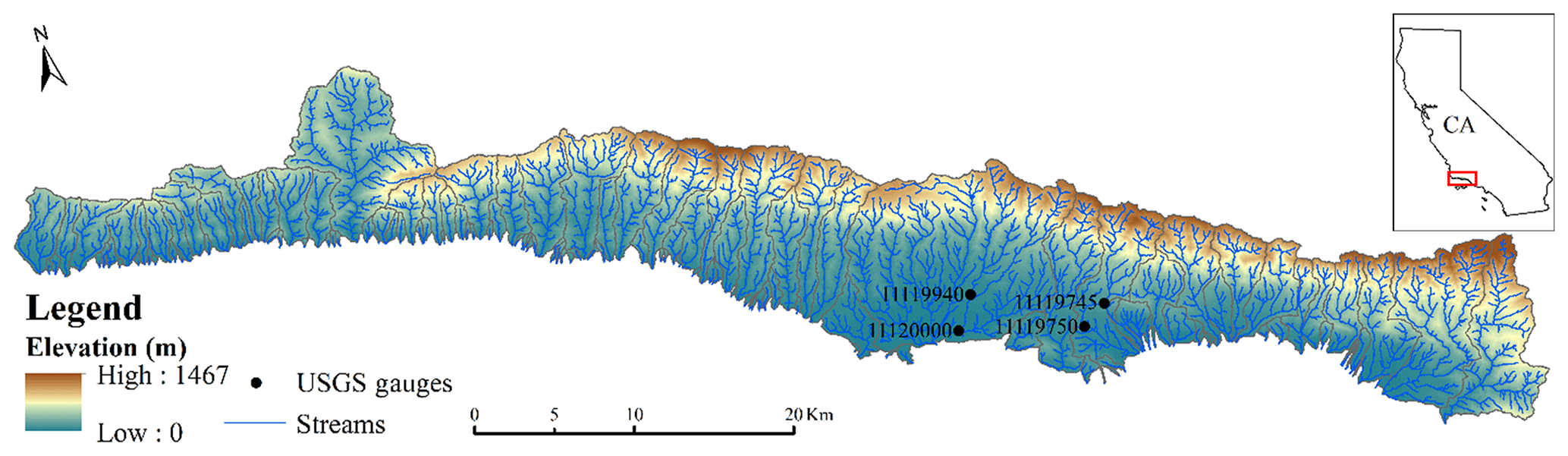
Figure 1Study region with USGS streamflow gauges. The inset figure indicates the location of SBC in the state of California (CA).
2.2 Data
Daily precipitation and temperature with a spatial resolution of (roughly 6 by 6 km) (Livneh et al., 2015), and daily streamflow from four USGS gauges for the period 1984–2013 were used to calibrate and validate the hydrologic models. The Global Soil Dataset for use in Earth system models (GSDE) was used to estimate saturated hydraulic conductivity and saturated moisture content. The 16 d composite albedo product (MCD43C3) with a spatial resolution of and the monthly aerosol optical depth product (MOD08M3) with a spatial resolution of , both derived from NASA's Moderate Resolution Imaging Spectroradiometer (MODIS), were used to determine net radiation for evapotranspiration (PET) estimation. The aerosol optical depth product was downscaled to (Raoufi and Beighley, 2017).
For the historical (1986–2005) and future climate simulations (2081–2100), downscaled precipitation and temperature from 10 climate models (please refer to Pierce et al., 2014, and Pierce et al. ,2015, for model details) in the Coupled Model Inter-Comparison Project, Phase 5, (CMIP5) (Taylor et al., 2012) for two emission scenarios, RCP 4.5 and RCP 8.5 (Moss et al., 2010), were used. These 10 GCMs were selected because they have the best performance in representing historical climate dynamics at southwest U.S. and California state scales (Pierce et al., 2018).
2.3 Hydrologic modeling framework
2.3.1 Hydrologic model development
This modeling framework was developed on the basis of the Hillslope River Routing model (HRR) (Beighley et al., 2009). The watersheds were delineated using the digital elevation model (DEM) data with a resolution of 3′′ (∼90 m at the Equator) (Yamazaki et al., 2017). The sub-basins were irregular-shape catchments defined by the flow accumulation area threshold. In this study, the threshold was 1 km2, which means the sub-basins (model units) were a size of roughly 1 km2. The hydrogeological inputs of hydrologic models, including surface roughness, saturated hydraulic conductivity, soil thickness, porosity, plane slope, channel slope, and channel roughness, were averaged over each sub-basin. This indicates these parameters were averaged for each model unit, the majority of which has an area of roughly 1 km2, with less than 1 % having an area of <1 km2. The geometry of each sub-basin (plane length and width) was calculated based on an “open-book” assumption, which assumes each sub-basin is a rectangle divided by the river channel into two identical parts like an open book. Please refer to Beighley et al. (2009) for more details. The grid-based potential ET (PET) was estimated using the method of Raoufi and Beighley (2017). The precipitation and PET were extracted for each sub-basin using an area-weighted average method. Then the water-balance model (i.e., runoff generation method) was applied to each model unit to simulate runoff generation processes. Here, three runoff generation methods, runoff coefficient (Feng et al., 2019) and the methods used in variable infiltration capacity (VIC) (Wood et al., 1992; Liang et al., 1996) and simple-TOPMODEL model (Niu et al., 2005; Beven, 2000; Beven et al., 1995), were used to simulate the generation of surface and subsurface runoff excess. The routing methods within the HRR model (i.e., kinematic wave for surface and subsurface lateral routing and Muskingum–Cunge for channel routing) were used to simulate the transport of runoff excess. To clarify, we denote the three runoff generation algorithms, runoff coefficient, runoff generation method used in variable infiltration capacity and runoff generation method used in simple-TOPMODEL, as RCM, VIC, and STP, respectively. Three hydrologic models which integrate one of these runoff generation methods with the HRR routing model are referenced as RCM-HRR, VIC-HRR, and STP-HRR, respectively. The differences between simulations from these three models were considered to be the uncertainty resulting from hydrologic models. The three runoff generation algorithms were described in the Supplement.
The water movement between soil layers in the soil matrix was similar to that in the modified VIC-2L model (Liang et al., 1996). The soil was divided into two layers: upper layer (0.6 m) and lower layer (1.2 m). The soil thickness data were from the Soil Survey Geographic (SSURGO) Data Base for Santa Barbara County (NRCS, 1995). After the surface runoff was determined, the infiltrated water was added to the upper soil layer, and the soil moisture was updated. If the upper soil was oversaturated, the excess water was returned to the surface. The evapotranspiration was estimated using Eq. (S15) in the Supplement. The interaction between the upper and lower soil layers was simulated using the Clapper–Hornberger equation (Eqs. S16–S17). Subsurface runoff was generated from the bottom of the lower soil layer. After the water fluxes (runoff, ET, and water movement between soil layers) were determined, the soil moisture was updated, which would be used for the water balance calculation in the next time step. After water excess for surface and subsurface runoff was quantified, the kinematic wave approach was applied to simulate the transport of runoff from the planes (surface and subsurface), and the Muskingum–Cunge method was used for channel routing following the conservation equations (Eqs. S18–S20) (Beighley et al., 2009). Two conceptual parameters, Ks_all and Kss_all, were used in the routing model to account for spatial heterogeneity at the model unit scale and uncertainties in the hydro-geologic inputs associated with the plane routing processes (e.g., surface roughness and saturated hydraulic conductivity). A conceptual illustration of the hydrologic models is shown in Fig. 2.
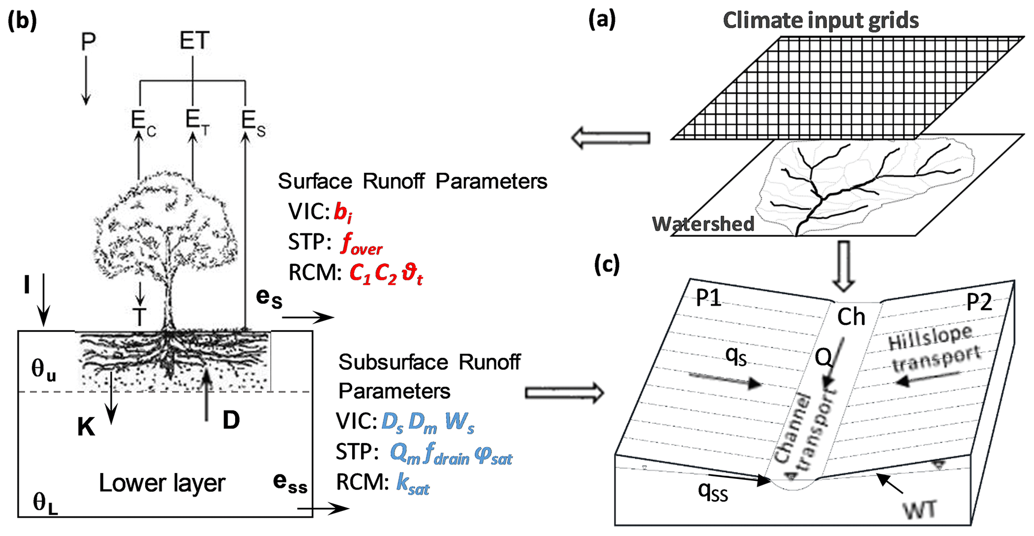
Figure 2The conceptual framework of the hydrologic models used in this study. Portions of this figure were adapted from the work of Beighley et al. (2009). (a) shows the grid-based climate inputs for hydrologic models; (b) shows water balance models; P is precipitation; ET is evapotranspiration; Es is soil evaporation; Ec is canopy evaporation; ET is transpiration; es is water available for surface runoff; ess is water available for subsurface runoff; θU is relative soil moisture in the upper soil layer; θL is relative soil moisture in lower soil layer; I is infiltration; K is water flux from the upper layer to the lower layer; and D is diffusive water flux from the lower layer to the upper layer; (c) shows the HRR routing model; the “open-book” assumption: two identical planes (P1 and P2) with the channel (Ch) in the center of each sub-basin; qs is surface runoff; qss is subsurface runoff; Q is discharge in the river channel, and WT is the groundwater table. The parameters in red italic are for surface runoff generation; the parameters in blue italic are for subsurface runoff generation. The first columns in the tables indicate the models that the parameters are used for. The definition of these parameters can be found in the Supplement.
2.3.2 Model calibration
After the models were set up, a state-of-the-art optimization algorithm, the Borg Multiobjective Evolutionary Algorithm (Borg MOEA) (Hadka and Reed, 2013), was adopted to optimize the model parameters (Table 1). The models were spun up for 1 year to ensure the equilibrium status. For each model, there were four parameters calibrated for runoff generation processes and two parameters calibrated for routing processes. Ks_all and Kss_all are conceptual parameters, and they can be different for different model structures even for the same study region. Therefore, they were calibrated for each model separately. The Nash–Sutcliffe model efficiency coefficient (NSE) (Eq. 1) was used to assess model performance, as it accounts for model performance in terms of both timing and magnitudes of peak flow and base flow that are particularly important in this study. The optimal parameter set was determined after the improvement of error was minimized (here it was defined as ΔNSE<0.005).
where and are simulated and observed discharge at time t, respectively (m3 s−1), and is the mean observed discharge during the study period of length T (m3 s−1).

To quantify the uncertainties from model parameters, we selected 10 parameter sets using the following criteria: (1) select 4 parameter sets with the highest NSE based on the calibration results; (2) rank the remaining parameter sets based on their performance (i.e., NSE) and randomly select 6 sets from the top 20 % candidates. This parameter selection process enabled us to take both parameter dominance and variability into account while maintaining the high model performance, which is important for the uncertainty analysis. These 10 parameter sets were then used for uncertainty analysis.
2.4 Uncertainty analysis
The uncertainty was quantified by running each of the 30 hydrologic model-parameter sets (i.e., 3 hydrologic models and 10 parameter sets, ) with each of the 20 forcing sets (i.e., 10 GCMs and 2 emission scenarios, ) for a total of 600 simulations. Here, we used GCM outputs as the forcings of hydrologic models for both historical (1986–2005) and future (2081–2100) periods. For each simulation scenario (i.e., the combination of hydrologic model, parameter set, GCM, and RCP), the historical and future daily streamflow and runoff were simulated and the relative changes (%) were quantified. Note that there is no RCP for the historical period, and we used the same historical simulation for RCP 4.5 and 8.5. To evaluate the uncertainty sources and their relative significance in these simulated changes in runoff, discharge, and seasonality for the future period, the analysis of variance (ANOVA) (Vetter et al., 2015; Addor et al., 2014; Hattermann et al., 2018; Chegwidden et al., 2019) was used. The contribution of each uncertainty source for a variable of interest (e.g., monthly runoff, 100-year flood discharge, or the duration of the wet season) was defined as the fraction of its variance to the total variance. The total variance was quantified as the total sum of squares (SStotal) of differences between the simulations and the mean of all simulations (Eq. 2):
where qijkl is the simulated value of the variable of interest by the ith hydrologic model with the jth parameter set, forced by the kth GCM projection under the lth RCP scenario; qoooo is the overall average of the simulated variable. Next, the SSTotal can be divided into 15 parts representing the four main effects (or first-order effects) and six second-order, four third-order, and one fourth-order interaction effects. For clarity, the third and fourth orders of interaction effects were combined and represented as SS3.4 in Eq. (3).
where SSHyd, SSpara, SSGCM, and SSRCP are the main effects (i.e., uncertainties or variance) from hydrologic models, hydrologic model parameters, GCMs and RCPs, respectively; SSHyd.para, SSHyd.GCM,SSHyd.RCP, SSpara.GCM, SSpara.RCP, and SSGCM.RCP are uncertainties from interactions between the hydrologic models and parameterization, hydrologic models and GCMs, hydrologic models and RCPs, parameterization and GCMs, parametrization and RCPs, and GCMs and RCPs, respectively. The calculation of each order is illustrated in Eqs. (S21)–(S23).
To avoid bias from the difference in sample sizes of uncertainty sources (i.e., 3 hydrologic models, 3 parameter sets, 10 GCMs and 2 RCPs), a subsampling step was performed by following Vetter et al. (2015). In the subsampling step, 2 samples (i.e., the minimum number of uncertainty sources, here RCPs) from each source were randomly selected, that is, 2 hydrologic models, 2 parameter sets, 2 GCMs, and 2 RCPs, which indicates that NHyd, Npara, NGCM, and NRCP in Eqs. (2) and (S21)–(S22) are all equal to 2. This generated subsamples. For each subsample, the fractional sum of squares was calculated for each effect using Eqs. (S21)–(S23), and then the average of variance fractions of each source is used as the uncertainty contribution from that source using Eq. (S24).
2.5 Probability of estimated changes
In addition to quantifying uncertainties and associated contributions from different sources, an evaluation of the probability of uncertain changes in discharge can be useful to provide actionable information for the stakeholders such as water-resource managers. In this study, Bayesian model averaging (BMA) (Duan et al., 2007) was used to evaluate the model performance in reproducing historical hydrologic conditions, and then weights were assigned to each of them based on their performance. A model with better performance was assigned a higher weight, assuming it has a higher probability of representing the truth. Note that there is no RCP for the historical period, so only combinations of hydrologic models, parameter sets and GCMs () were evaluated. Here the models' performance in representing annual mean discharge (Qm) and annual maximum daily discharge (Qp) is evaluated. Here, the annual mean discharge was defined as the average of daily streamflow in a year. In this study region, there is typically no rain for most times of a year, and it is not uncommon in such a Mediterranean climate region that the annual runoff is mainly generated from one major storm event. Therefore, the annual mean/max series are representative of the characteristics of the discharge dynamics. The details of this procedure can be found in the Supplement. After the weights of model ensemble were obtained using the BMA method, the statistics of posterior probability distribution (here it was assumed to be normal distribution) of estimated changes in Qm, Qp, and Q100 in the future (2081–2100) relative to the historical period 1986–2005 were calculated using Eqs. (S29)–(S34).
2.6 Definition of hydrologic seasonality
To quantify the onset and duration of hydrologic seasons, we calculated the accumulative discharge in the whole basin for each water year. Then the day showing the 10 % of accumulative annual discharge was defined as the onset of the wet season, and the number of days between 10 % and 90 % of the accumulated discharge series was defined as the duration of the wet season.
3.1 Hydrologic model performance
The three hydrologic models performed well in representing streamflow dynamics in the study region. The NSE varies within 0.56–0.67 and 0.53–0.62 for the calibration and validation periods, respectively, in Mission Creek (USGS gauge no. 11119750) (Fig. 3). At other calibrated watersheds, the models perform similarly well, with NSE varying between 0.45 and 0.60 for the calibration period and between 0.42 and 0.62 for the validation period (Figs. S1–S3 in the Supplement). Simulated streamflow from the three models matches the in situ measurements in both magnitudes and timing of hydrographs at event scales (Fig. 3b). At annual scale, simulated annual peak flows are comparable to the observations in most years. However, in some years with extreme events, for example in January 1995, February 1998, and January 2005 (highlighted in Fig. 3c), the simulated peaks are much lower than the gauge records. This disparity can be attributed to the input bias (e.g., precipitation or streamflow measurements). This was identified using an “extreme scenario” simulation, which assumed 100 % precipitation is transformed to surface runoff (i.e., without any loss due to, for example, infiltration or evapotranspiration) and transported immediately to river channels and represents the maximum streamflow considering groundwater is minimal in the study region (Beighley et al., 2003). Even in this extreme scenario, the simulated peaks were still lower (events highlighted in red in Fig. 3c) or slightly higher (event highlighted in blue in Fig. 3c) than the gauge observations. This is likely because model forcings are biased low for these events. One possible source of this bias can be the grid-based precipitation dataset which averages the precipitation rates over the grid masking spatial heterogeneity and thus reducing precipitation rates at some locations. The uncertainties in gauge measurements can also be a bias source. For example, in typical conditions the uncertainty in streamflow measurements ranges between 6 % and 19 % in small watersheds, but it can be higher during large storm events when accurate stage measurements are more difficult (Harmel et al., 2006). Beighley et al. (2003) also identified the overestimation of gauge records for the 1995 January event at gauge 11119940. As for mean annual discharge, all three models tend to overestimate it for the study period, mainly due to the overestimation of subsurface flow during dry seasons (Fig. 3d). This highlights challenges in simulating hydrologic processes in semiarid regions under a Mediterranean climate.
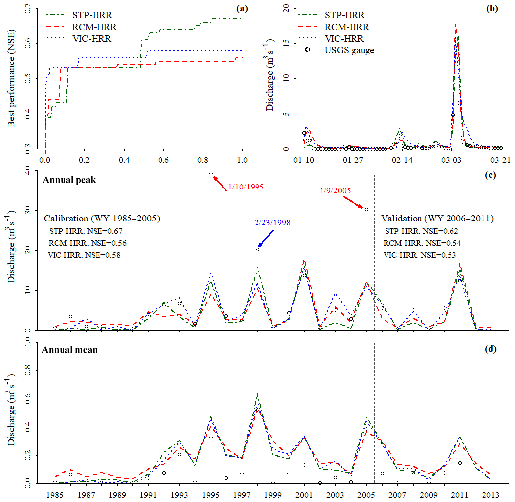
Figure 3Model performance for calibration and validation periods: (a) model performance (assessed by NSE) during the calibration process; the x axis is the normalized calibration process; the “normalized calibration process” means the x axis range is normalized by the number of iterations during calibration; (b) hydrographs simulated by three calibrated models and measured by the USGS gauge; in order to show the details of the hydrographs, they are zoomed in to the wet season in 2001; the model performance is similar in other years; (c) simulated annual peak flow during calibration (water year 1985–2005) and validation (water year 2006–2011) periods as compared with in situ observations; black texts indicate model performance (i.e., NSE); the points highlighted in red arrows indicate the events were not reproduced by models due to the input (e.g., precipitation or discharge observation) bias; the point highlighted in blue arrow is similar to those in red but at a lower probability; and (d) simulated and observed annual mean flow during calibration and validation periods. For clarity, only results for the Mission Creek watershed (USGS gauge no. 11119750) are shown here; results for other gauged watersheds are similar and can be found in the Supplement (Figs. S1–S3).
Among the three hydrologic models, STP-HRR has the best overall performance (i.e., highest average NSE), mainly due to its better ability to capture flood peaks than the other two models (Figs. 3, S1–S3). The peak performance is likely a result of the STP-HRR representing the runoff generation process as an exponential relationship between soil moisture and runoff rates, which makes runoff generation more sensitive to soil moisture dynamics as compared to the other two models. This algorithm is well suited to representing the significant nonlinearity of hydrologic response to rainfall in the study region. RCM-HRR and VIC-HRR have similar overall performance (i.e., similar average NSE); however, they represent hydrologic dynamics differently. VIC-HRR tends to perform better in representing small peak flows than RCM-HRR but worse in simulating mean flow (or total discharge volume) (Figs. 3, S1–S3). This is because as the wet season proceeds, the lower soil layer is close to saturation (i.e., relative soil moisture is higher than the threshold Ws for VIC-HRR), which initiates the quadratic relationship between soil moisture and subsurface runoff in VIC-HRR. This quadratic response to soil moisture conditions can lead to much higher subsurface runoff (1–2 orders of magnitude higher than that of RCM-HRR), which contributes to the lower performance in reproducing the total volume of discharge. This also explains that VIC-HRR generates the highest subsurface runoff during the wet season (Fig. 4). In addition, VIC-HRR also generates the most surface runoff during the wet season (Fig. 4). This is because when soil is almost saturated, surface runoff in VIC-HRR is almost a linear function of precipitation with a coefficient of 1 (much larger than RCM-HRR, which is 0.2 (C2), and STP-HRR, which is around 0.5 depending on the watershed topography). The higher surface and subsurface runoff generated by VIC-HRR lead to the overestimation of mean annual flow (Fig. 3d). However, there are no in situ measurements of surface and subsurface runoff fluxes, and it is difficult to evaluate model performance for these quantities. In Fig. 4, the simulated surface and subsurface runoff from National Land Data Assimilation Systems VIC model (NLDAS-VIC) (Xia et al., 2012) outputs are shown for the purpose of comparison. The NLDAS-VIC runoff simulations are from the same runoff generation model (i.e., VIC) as used in this work and have similar spatial/temporal resolutions to those in this study, which makes it a suitable reference for comparison. A similar pattern, i.e., a very high subsurface runoff, even higher than surface runoff, during the wet season, can be found from NLDAS-VIC simulations. The surface runoff of NLDAS-VIC is lower than those generated by the models in this study, which is probably because of the difference in precipitation inputs. The NLDAS precipitation input is lower during the wet season than that used in this study for the study region. In addition, the difference in spatial resolutions of precipitation (0.125∘ for NLDAS vs. 0.0625∘ for this study) can also contribute to the difference in simulated runoff.
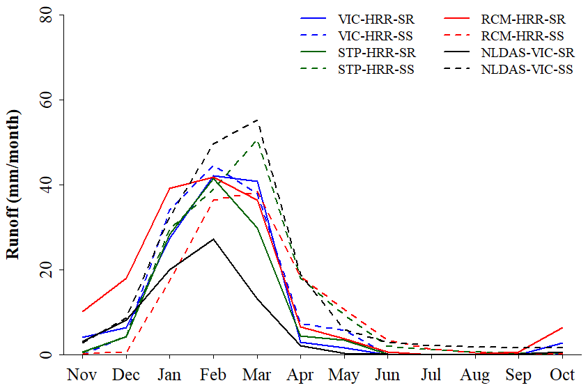
Figure 4Simulated monthly surface and subsurface runoff for the Mission Creek watershed (USGS gauge no. 11119750) by three models for the calibration period (water year 1985–2005). Surface runoff is denoted by “SR” and subsurface runoff is denoted by “SS” in this figure. Monthly surface and subsurface runoff from National Land Data Assimilation Systems (NLDAS) VIC model simulation for the same period are shown here for comparison purposes.
These results may suggest that STP-HRR is more suitable than VIC-HRR in representing hydrologic processes in Mediterranean regions, where 80 % of annual precipitation is concentrated in a short period (roughly 3 months). As the wet season proceeds, the soil is close to saturation conditions, under which the saturation excess overland flow is dominant. That explains why STP-HRR performs best in this study region. VIC-HRR is probably more suitable to the regions where precipitation events are sparsely distributed where soil is not easy to get saturated. Although RCM is an empirical method, it performs fairly well in this study, mainly because it captures the nonlinearity of hydrologic processes through a switch between dry and wet surface runoff coefficients (C1 and C2) based on the soil moisture conditions.
Ten sets of parameters were selected for each model (Fig. 5). Most optimal parameter sets (red circles in Fig. 5) are very close, except for C1, Ks_all in RCM-HRR and Ks_all, Ds in VIC-HRR, suggesting that most parameters are important factors controlling model performance. For the randomly selected parameters (green circles in Fig. 5), most of them spread over the whole range, suggesting sufficient space for uncertainty analysis.
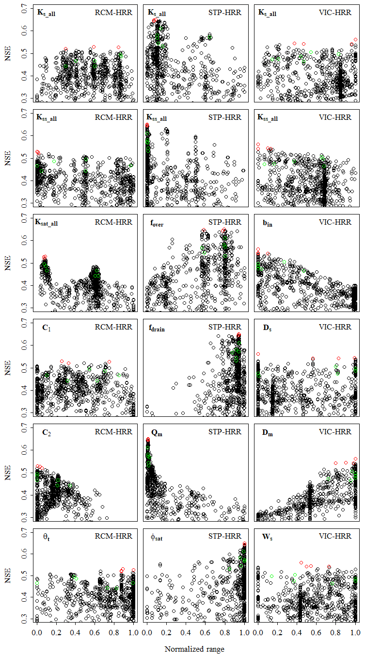
Figure 5Parameters (black circles) sampled during the calibration process and their corresponding performance (assessed by NSE). The red circles indicate the four parameter sets with the highest NSE values, and the green circles indicate six randomly selected parameter sets from the top 20 % samples (ranked by NSE). These 10 parameter sets were used for uncertainty analysis. In this figure, the parameter values are normalized by their ranges (shown in Table 1), so the range of the x axis is 0–1. The parameters were sampled throughout their whole ranges; however, for clarity, samples with NSE lower than 0.3 are not shown in this figure.
3.2 Impacts and uncertainty analysis
The projected changes in monthly runoff (surface, subsurface, and total) during 2081–2100 compared to the 1986–2005 range between −100 % and 300 % (Fig. 6a). The median changes indicate that surface runoff will probably increase in February and March and decrease in other months (Fig. 6a). This is because in the future, the onset of the wet season will be delayed and more severe storm events will occur during the shorter wet season (mainly during February and March) (Feng et al., 2019). The decrease in subsurface runoff in all months is probably because of the decrease in the frequency (or total number) of storm events (Feng et al., 2019). The changes in monthly total runoff show a similar pattern to the surface runoff, suggesting the more pronounced changes in surface runoff as compared to subsurface runoff. The major uncertainty sources are GCM and RCP, which account for ∼45 % of the total uncertainty (Fig. 6b). Hydrologic models contribute ∼10 % of the total uncertainty (Fig. 6b). This suggests that the climate patterns (e.g., storm event frequency and intensity) are more important factors controlling the runoff generation than the hydrologic model algorithms.

Figure 6(a) Projected relative changes (%) in monthly surface runoff, subsurface runoff, and total runoff in the whole study region during 2081–2100 as compared to the historical period (1986–2005); (b) relative contributions (%) of the uncertainties for the projected changes in the monthly total runoff; Hydro: hydrologic models; Para: hydrologic model parameters; GCM: general circulation model; RCP: representative concentration pathway (emission scenarios); “other” is the uncertainty from the third and fourth orders of interactions between the four major sources (i.e., GCMs, RCPs, hydrologic models, and parameters).
For the 28 major watersheds in SBC, the projected changes in Qm during 2081–2100 as compared to the historical period 1986–2005 range from −100 % to 220 % (Fig. S4). The median changes for each of these major watersheds are slightly above 0 %, varying between 1 % and 8 %. The major uncertainty sources are GCM and RCP, which account for ∼54 % of the total uncertainty. Among the first-order factors (i.e., GCM, RCP, hydrologic model, and parameterization), hydrologic model ranks third after GCM and RCP, accounting for 10 %–15 % of total uncertainty. In contrast, parameterization only induces less than 2 % of the total uncertainty. The remaining 25 %–35 % uncertainty is from the second-, third-, and fourth-order interactions between the four major sources. The projected relative changes in Qp and Q100 are similar in magnitude, both varying from −90 % to 250 % (Figs. S5 and 7). The median changes in Qp and Q100 for each watershed are higher than those of Qm, ranging between 10 % and 40 %. For most of the watersheds, GCM and RCP are the two major uncertainty contributors for Qp and Q100, accounting for ∼45 % of total uncertainties. The hydrologic model contributes ∼14 % of total uncertainties in Qp and Q100. Compared to Qm, Qp and Q100 get more uncertainty from the hydrologic models, which is likely due to highly nonlinear rainfall–runoff behavior and larger differences between runoff generation methods in generating peak flows as compared to average flow conditions.
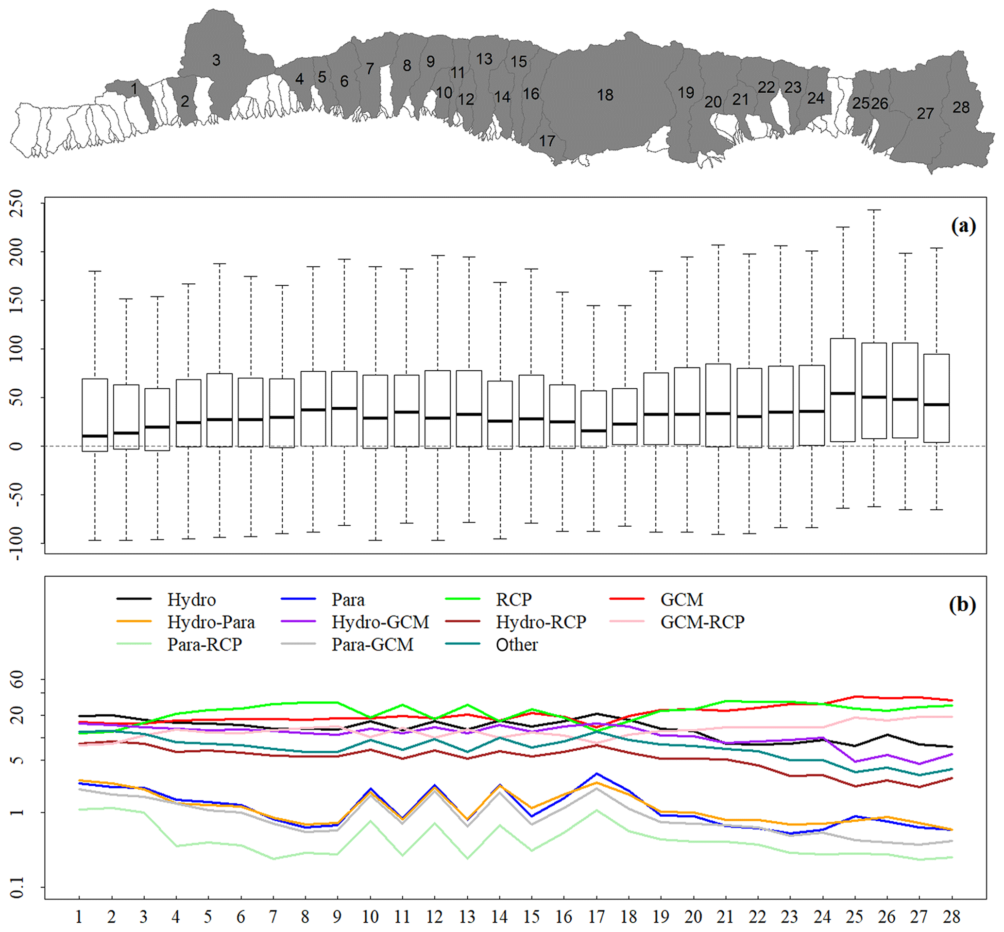
Figure 7(a) Projected relative changes (%) in 100-year flood discharge (Q100) in the major SBC watersheds (indicated by the grey watersheds in the map) during 2081–2100 as compared to the historical period (1986–2005); each bar depicts relative changes in minimum, maximum, median, and the 1st and 3rd quartiles for the ensemble outputs; bars from left to right spatially correspond to watersheds from west to east. For clarity, only watersheds with drainage areas larger than 7 km2, which account for roughly 83 % of the study area, are shown. (b) Relative contributions (%) of the uncertainties in the projected changes at each of these watersheds; Hydro: hydrologic models; Para: hydrologic model parameters; GCM: general circulation model; RCP: representative concentration pathway (emission scenarios); “other” is the uncertainty from the third and fourth orders of interactions between the four major sources (i.e., GCMs, RCPs, hydrologic models, and parameters).
Changes in Qm, Qp, and Q100 are higher under RCP 8.5, but the uncertainties are also higher (Fig. 8), which suggests the higher contribution of RCP 8.5 in the uncertainties of higher-order interactions between RCP and other factors (i.e., GCM, hydrologic model, and parameters). In Mission Creek watershed (USGS gauge no. 11119750), the probability of increase in Qm under RCP 4.5 is only 51 %. However, this probability increases to 64 % under RCP 8.5. For the less frequent events (Qp and Q100), the probabilities of positive changes are higher: 78 % and 85 % for Qp and Q100, respectively, under RCP 8.5. This implies that if RCP 8.5 happens in the future, the extreme events will probably get intensified.
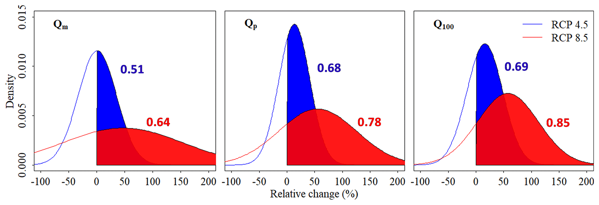
Figure 8Probability of changes in Qm, Qp, and Q100 at the Mission Creek watershed (no. 20 in the Fig. 7 map). The numbers in the plot are the probabilities of positive changes in Qm, Qp, and Q100 (areas of shaded regions) under each emission scenario (blue numbers are for RCP 4.5 and red numbers are for RCP 8.5).
Consistent with the work of Feng et al. (2019), this study suggests a delayed onset and shorter duration of the wet season (Fig. 9a). The median changes show that the wet season will start later by 3 d and become shorter by ∼6 d. The major uncertainty sources for both onset and duration of the wet season are GCM (∼20 %) and hydrologic models (∼15 %). Different from discharge and runoff, the seasonality shows more uncertainty from hydrological models (15 % vs. 12 %) and model parameters (∼6 % vs. 2 %) (Fig. 9b). This is because the seasonality integrates the runoff generation, paths, and transport processes for both surface and subsurface runoff, which are important for the timing and quantity of simulated discharge.
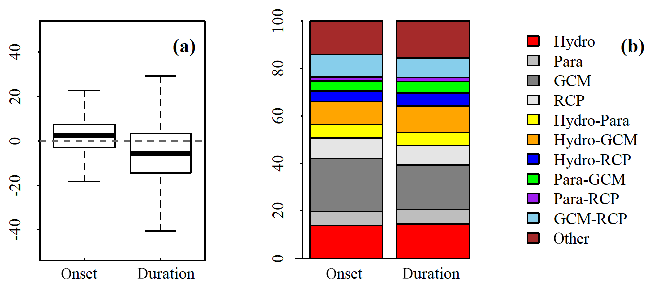
Figure 9(a) Projected change (days) in the onset and duration of the wet season in SBC; positive (negative) values indicate later (earlier) onset or longer (shorter) duration of the wet season; (b) relative contributions (%) of the uncertainties of the projected changes in seasonality. Hydro: hydrologic models; Para: hydrologic model parameters; GCM: general circulation model; RCP: representative concentration pathway (emission scenarios); “other” is the uncertainty from the third and fourth orders of interactions between the four major sources (i.e., GCMs, RCPs, hydrologic models, and parameters).
As the major carrier of nutrients/sediment, surface runoff and discharge are crucial for beach ecosystems in the study region (Myers et al., 2019; Aguilera and Melack, 2018). Nutrients and sediment build up over land surface and in channels during the dry season and get flushed with the initiation of the wet season (Scott and Williams, 1978; Keller and Capelli, 1992; Bende-Michl et al., 2013; Aguilera and Melack, 2018). The nutrients/sediment fluxes are positively correlated with hydrologic variability, and the majority of them occurs at the beginning of the wet season (Aguilera and Melack, 2018; Homyak et al., 2014). Therefore, both timing and magnitude of runoff and discharge will impact the nutrients/sediment export to the coastal ecosystems. The findings in this study reveal that the surface runoff and river discharge (especially the extremes) will increase but get delayed during the wet season (Figs. 6 and 9), implying that the nutrients/sediment fluxes will likely increase and occur in a shorter and delayed period. The decrease in runoff (both surface and subsurface) during the dry season suggests that the soil moisture will be lower under future climate conditions in the study region. The longer and drier dry season will probably increase the occurrence of severe droughts and wildfires.
Compared to previous studies (e.g., Vetter et al., 2015, Schewe et al., 2014; Hagemann et al., 2013; Troin et al., 2018; and Asadieh and Krakauer, 2017), this work identifies relatively low uncertainty contributions from hydrologic models. The main reason for this is probably that the hydrologic model uncertainty in this study was only from runoff generation algorithms and associated parameters. As is, the three hydrologic models share common algorithms for ET and plane/channel routing and the same model configuration (e.g., soil matrix and model unit definition). These similarities among models likely reduced the differences in simulated runoff and discharge. In addition, the uniform calibration approach and parameter selection criteria were also likely to eliminate user/method bias, which is common in studies that consider more than one hydrologic model. In contrast, the hydrologic models used in previous studies have their own model component algorithms (e.g., ET and routing algorithms) and model configurations. For example, the VIC model (here VIC refers to the original VIC model and is different from the model used in this study; to clarify, in the following text, VIC refers to the original VIC model, while VIC-HRR refers to the model used in this study) applies an ET algorithm different from the one used in this study (Raoufi and Beighley, 2017), uses the grid-based model units, ignoring the spatial arrangement, and has its own routing scheme which adopts the synthetic unit hydrograph concept. When comparing models owning their own component algorithms, the differences between models likely resulted in larger uncertainties in the simulation from hydrologic models in previous studies.
This study can also provide useful information for hydrologic model evaluation and selection. As discussed in Sect. 3.1, the STP-HRR model is more suitable than the other two models for the study region, mainly due to its ability to represent the highly nonlinear hydrological response to precipitation forcings. This implies hydrologic models adopting the saturation excess runoff generation algorithms may be more suitable for areas with a Mediterranean climate. The uncertainties from hydrologic models are larger than those from the hydrologic model parameters for all variables (i.e., discharge, runoff and seasonality), suggesting the inter-model variability is larger than the intra-model variability (from model parameters). This implies that model selection is more important than the parameter selection and that the parameter equifinality (or non-uniqueness) is less of a concern when quantifying climate change impacts on hydrologic fluxes using an ensemble of GCM forcings. In this study, only the runoff generation algorithm was investigated. Other hydrologic model components, such as ET algorithms and routing methods, also have variants. The choice of these components may also make a difference in the total uncertainties in simulated runoff and streamflow. In addition, the methods for GCM downscaling can also contribute to the uncertainty in predicted changes in hydrology. Further study integrating different algorithms for hydrologic model components as well as GCM downscaling methods can be conducted in the future. Such analysis can be useful to guide stakeholders to select appropriate hydrologic algorithms and to develop actionable adaptation and mitigation strategies to accommodate climate change.
This is the first study investigating hydrologic model uncertainty solely from runoff generation algorithms for a region with a Mediterranean climate. The framework developed in this study can be potentially used to identify the internal uncertainties of hydrologic models, i.e., uncertainties from hydrologic model components (e.g., runoff generation algorithms, ET algorithms, and routing models), which is particularly important for assessing model performance and quantifying the relative roles of different components in the uncertainty of simulations. This study region is a representative Mediterranean area characterized by dry summers and wet winters. This climate pattern and the highly nonlinear relationship between climate and hydrology significantly impact local society, agriculture, and ecosystems, as discussed before. The findings in this study, including the favorability of the STP algorithm, the important role of GCM selection, and the negligible role of hydrologic model parameters in the uncertainty, can be useful for studies associated with hydrologic model evaluation and climate change impact analysis for other Mediterranean regions.
A modeling framework which integrates multiple runoff generation algorithms (VIC, STP, and RCM) with the HRR routing model was developed. Forced with an ensemble of GCM outputs under different emission scenarios, this framework is able to quantify the climate change impacts on surface and subsurface runoff, streamflow, and hydrologic seasonality and evaluate the associated uncertainties from different sources (i.e., RCPs, GCMs, hydrologic process models and parameterization). The results show that the surface runoff will likely increase in February and March while decrease in other months, and the subsurface runoff will likely decrease due to changes in the patterns of storm events. The median changes in mean annual discharge for the major watersheds in SBC are 1 %–8 %, with an uncertainty of 320 % (here, uncertainty refers to the range of predicted relative changes among models, that is, from −100 % to +220 %); the median changes in annual peak discharge and 100-year flood discharge are higher than those of mean annual discharge, varying between 10 % and 40 %, but with a higher uncertainty of 340 % (−90 % to +250 %). The results based on the BMA analysis indicate that there is a high probability (up to 85 %) that streamflow, especially the extreme quantities (e.g., Q100) under RCP 8.5, will increase. The seasonality analysis shows that the wet season will be delayed (by 3 d, median) and shortened (by 6 d, median). For the uncertainties in the projected changes in runoff and discharge, GCM and RCP are the top two contributors, accounting for roughly 50 % of total uncertainties at most major watersheds in SBC, while hydrologic process models (i.e., runoff generation modules) contribute ∼12 % on average, with the remaining 30 %–40 % of the uncertainty coming from the interactions between these individual sources. Hydrologic model parameters alone contribute less than 2 % of the uncertainty. In contrast, for the changes in seasonality, the uncertainty contributions from hydrologic models (∼15 %) and hydrologic model parameters (∼6 %) are higher as compared to those for runoff and discharge, making GCMs and hydrologic models the two major uncertainty sources.
Unique to the framework in this study, the uncertainties from different hydrologic model components (e.g., runoff generation process) and associated model parameterizations can be identified and quantified. The results can be useful for practices and studies in many fields, e.g., water resources, risk controls, and ecosystem conservation, for the study region as well as other Mediterranean regions.
The source code and dataset supporting this work are available on Github: https://github.com/dongmeifeng-2019/HydroUncertainty (last access: 10 April 2020) (Feng, 2020).
The supplement related to this article is available online at: https://doi.org/10.5194/hess-24-2253-2020-supplement.
DF designed the experiments, developed the models, performed the simulations, and prepared the manuscript. EB conceptualized the project and reviewed and edited the manuscript.
The authors declare that they have no conflict of interest.
This research was supported by the Santa Barbara Area Coastal Ecosystem Vulnerability Assessment (SBA CEVA) with funding from the NOAA Climate Program Office Coastal and Ocean Climate Applications (COCA) and Sea Grant Community Climate Adaptation Initiative (CCAI) and the National Science Foundation's Long-Term Ecological Research (LTER) program (Santa Barbara Coastal LTER – OCE9982105, OCE-0620276 and OCE-123277). The authors thank David Hadka at Pennsylvania State University and Chinedum Eluwa at University of Massachusetts, Amherst, for their help with setting up the Borg MOEA. The authors acknowledge editor Hilary McMillan, Konstantinos Andreadis and two anonymous reviewers for their valuable comments that significantly improved the manuscript.
This research has been supported by the National Science Foundation (grant nos. OCE9982105, OCE-0620276, and OCE-123277).
This paper was edited by Hilary McMillan and reviewed by two anonymous referees.
Addor, N., Rössler, O., Köplin, N., Huss, M., Weingartner, R., and Seibert, J.: Robust changes and sources of uncertainty in the projected hydrological regimes of Swiss catchments, Water Resour. Res., 50, 7541–7562, https://doi.org/10.1002/2014wr015549, 2014.
Aguilera, R. and Melack, J. M.: Relationships Among Nutrient and Sediment Fluxes, Hydrological Variability, Fire, and Land Cover in Coastal California Catchments, J. Geophys. Res.-Biogeosc., 123, 2568–2589, https://doi.org/10.1029/2017JG004119, 2018.
Alder, J. R. and Hostetler, S. W.: The Dependence of Hydroclimate Projections in Snow-Dominated Regions of the Western United States on the Choice of Statistically Downscaled Climate Data, Water Resour. Res., 55, 2279–2300, https://doi.org/10.1029/2018WR023458, 2019.
Asadieh, B. and Krakauer, N. Y.: Global change in streamflow extremes under climate change over the 21st century, Hydrol. Earth Syst. Sci., 21, 5863–5874, https://doi.org/10.5194/hess-21-5863-2017, 2017.
Barnett, T. P., Adam, J. C., and Lettenmaier, D. P.: Potential impacts of a warming climate on water availability in snow-dominated regions, Nature, 438, 303–309, 2005.
Beighley, R. E., Melack, J. M., and Dunne, T.: Impacts of California's climatic regimes and coastal land use change on streamflow characteristics, JAWRA J. Am. Water Resour. Assoc., 39, 1419–1433, https://doi.org/10.1111/j.1752-1688.2003.tb04428.x, 2003.
Beighley, E., Eggert, K. G., Dunne, T., He, Y., Gummadi, V., and Verdin, K. L.: Simulating hydrologic and hydraulic processes throughout the Amazon River Basin, Hydrol. Process., 23, 1221–1235, https://doi.org/10.1002/hyp.7252, 2009.
Bende-Michl, U., Verburg, K., and Cresswell, H. P.: High-frequency nutrient monitoring to infer seasonal patterns in catchment source availability, mobilisation and delivery, Environ. Monitor. Assess., 185, 9191–9219, https://doi.org/10.1007/s10661-013-3246-8, 2013.
Beven, K.: Rainfall-Runoff Modelling: The Primer, John Wiley, Chichester, 2000.
Beven, K. J. and Cloke, H. L.: Comment on “Hyperresolution global land surface modeling: Meeting a grand challenge for monitoring Earth's terrestrial water” by Eric F. Wood et al, Water Resour. Res., 48, W01801, https://doi.org/10.1029/2011WR010982, 2012.
Beven, K., Lamb, R., Quinn, P., Romanowicz, R., and Freer, J.: Topmodel, Computer Models of Watershed Hydrology, edited by: Singh, V. P., Water Resources Publications, Highlands Ranch, Colorado, 1995.
Cai, W., Borlace, S., Lengaigne, M., van Rensch, P., Collins, M., Vecchi, G., Timmermann, A., Santoso, A., McPhaden, M. J., Wu, L., England, M. H., Wang, G., Guilyardi, E., and Jin, F.-F.: Increasing frequency of extreme El Nino events due to greenhouse warming, Nature Clim. Change, 4, 111–116, https://doi.org/10.1038/nclimate2100, 2014.
Chegwidden, O. S., Nijssen, B., Rupp, D. E., Arnold, J. R., Clark, M. P., Hamman, J. J., Kao, S.-C., Mao, Y., Mizukami, N., Mote, P. W., Pan, M., Pytlak, E., and Xiao, M.: How Do Modeling Decisions Affect the Spread Among Hydrologic Climate Change Projections? Exploring a Large Ensemble of Simulations Across a Diversity of Hydroclimates, Earth's Future, 7, 623–637, https://doi.org/10.1029/2018ef001047, 2019.
Dai, A.: The influence of the inter-decadal Pacific oscillation on US precipitation during 1923–2010, Clim. Dynam., 41, 633–646, 2013.
Dettinger, M.: Climate change, atmospheric rivers, and floods in California – a multimodel analysis of storm frequency and magnitude changes, J. Am. Water Resour. Assoc., 47, 514–523, https://doi.org/10.1111/j.1752-1688.2011.00546.x, 2011.
Duan, Q., Ajami, N. K., Gao, X., and Sorooshian, S.: Multi-model ensemble hydrologic prediction using Bayesian model averaging, Adv. Water Resour., 30, 1371–1386, https://doi.org/10.1016/j.advwatres.2006.11.014, 2007.
Eisner, S., Flörke, M., Chamorro, A., Daggupati, P., Donnelly, C., Huang, J., Hundecha, Y., Koch, H., Kalugin, A., Krylenko, I., Mishra, V., Piniewski, M., Samaniego, L., Seidou, O., Wallner, M., and Krysanova, V.: An ensemble analysis of climate change impacts on streamflow seasonality across 11 large river basins, Climatic Change, 141, 401–417, https://doi.org/10.1007/s10584-016-1844-5, 2017.
Espinoza, V., Waliser, D. E., Guan, B., Lavers, D. A., and Ralph, F. M.: Global Analysis of Climate Change Projection Effects on Atmospheric Rivers, Geophys. Res. Lett., 45, 4299–4308, https://doi.org/10.1029/2017GL076968, 2018.
Feng, D.: HydroUncertainty, available at: https://github.com/dongmeifeng-2019/HydroUncertainty, last access: 10 April 2020.
Feng, D., Beighley, E., Hughes, R., and Kimbro, D.: Spatial and temporal variations in eastern U.S. Hydrology: Responses to global climate variability, JAWRA J. Am. Water Resour. Assoc., 52, 1089–1108, https://doi.org/10.1111/1752-1688.12445, 2016.
Feng, D., Beighley, E., Raoufi, R., Melack, J., Zhao, Y., Iacobellis, S., and Cayan, D.: Propagation of future climate conditions into hydrologic response from coastal southern California watersheds, Climatic Change, 153, 199–218, https://doi.org/10.1007/s10584-019-02371-3, 2019.
Giuntoli, I., Villarini, G., Prudhomme, C., and Hannah, D. M.: Uncertainties in projected runoff over the conterminous United States, Climatic Change, 150, 149–162, https://doi.org/10.1007/s10584-018-2280-5, 2018.
Hadka, D. and Reed, P.: Borg: An auto-adaptive many-objective evolutionary computing framework, Evolutionary Computation, 21, 231–259, 2013.
Hagemann, S., Chen, C., Clark, D. B., Folwell, S., Gosling, S. N., Haddeland, I., Hanasaki, N., Heinke, J., Ludwig, F., Voss, F., and Wiltshire, A. J.: Climate change impact on available water resources obtained using multiple global climate and hydrology models, Earth Syst. Dynam., 4, 129–144, https://doi.org/10.5194/esd-4-129-2013, 2013.
Harmel, R. D., Cooper, R. J., Slade, R. M., Haney, R. L., and Arnold, J. G.: Cumulative uncertainty in measured streamflow and water quality data for small watersheds, Transactions of the ASABE, 49, 689–701, 2006.
Hattermann, F. F., Vetter, T., Breuer, L., Su, B., Daggupati, P., Donnelly, C., Fekete, B., Flörke, F., Gosling, S. N., Hoffmann, P., Liersch, S., Masaki, Y., Motovilov, Y., Müller, C., Samaniego, L., Stacke, T., Wada, Y., Yang, T., and Krysnaova, V.: Sources of uncertainty in hydrological climate impact assessment: a cross-scale study, Environ. Res. Lett., 13, 015006, https://doi.org/10.1088/1748-9326/aa9938, 2018.
Homyak, P. M., Sickman, J. O., Miller, A. E., Melack, J. M., Meixner, T., and Schimel, J. P.: Assessing Nitrogen-Saturation in a Seasonally Dry Chaparral Watershed: Limitations of Traditional Indicators of N-Saturation, Ecosystems, 17, 1286–1305, https://doi.org/10.1007/s10021-014-9792-2, 2014.
Horton, R. E.: The Rôle of infiltration in the hydrologic cycle, Eos, Transactions American Geophysical Union, 14, 446–460, https://doi.org/10.1029/TR014i001p00446, 1933.
IPCC: Climate Change 2014: Synthesis Report. Contribution of Working Groups I, II and III to the Fifth Assessment Report of the Intergovernmental Panel on Climate Change, edited by: Pachauri, R. K. and Meyer, L. A., p. 151, IPCC, Geneva, Switzerland, 2014.
Kay, A. L., Davies, H. N., Bell, V. A., and Jones, R. G.: Comparison of uncertainty sources for climate change impacts: flood frequency in England, Climatic Change, 92, 41–63, https://doi.org/10.1007/s10584-008-9471-4, 2009.
Keller, E. A. and Capelli, M. H.: VENTURA RIVER FLOOD OF FEBRUARY 1992: A LESSON IGNORED?1, JAWRA J. Am. Water Resour. Assoc., 28, 813–832, https://doi.org/10.1111/j.1752-1688.1992.tb03184.x, 1992.
Liang, X., Wood, E. F., and Lettenmaier, D. P.: Surface soil moisture parameterization of the VIC-2L model: Evaluation and modification, Global Planet. Change, 13, 195–206, https://doi.org/10.1016/0921-8181(95)00046-1, 1996.
Livneh, B., Bohn, T. J., Pierce, D. W., Munoz-Arriola, F., Nijssen, B., Vose, R., Cayan, D. R., and Brekke, L.: A spatially comprehensive, hydrometeorological data set for Mexico, the U.S., and Southern Canada 1950–2013, Scientific Data, 2, 150042, https://doi.org/10.1038/sdata.2015.42, 2015.
Milly, P. C. D., Dunne, K. A., and Vecchia, A. V.: Global pattern of trends in streamflow and water availability in a changing climate, Nature, 438, 347–350, 2005.
Moss, R. H., Edmonds, J. A., Hibbard, K. A., Manning, M. R., Rose, S. K., van Vuuren, D. P., Carter, T. R., Emori, S., Kainuma, M., Kram, T., Meehl, G. A., Mitchell, J. F. B., Nakicenovic, N., Riahi, K., Smith, S. J., Stouffer, R. J., Thomson, A. M., Weyant, J. P., and Wilbanks, T. J.: The next generation of scenarios for climate change research and assessment, Nature, 463, 747–756, https://doi.org/10.1038/nature08823, 2010.
Myers, M. R., Barnard, P. L., Beighley, E., Cayan, D. R., Dugan, J. E., Feng, D., Hubbard, D. M., Iacobellis, S. F., Melack, J. M., and Page, H. M.: A multidisciplinary coastal vulnerability assessment for local government focused on ecosystems, Santa Barbara area, California, Ocean Coast. Manage., 182, 104921, https://doi.org/10.1016/j.ocecoaman.2019.104921, 2019.
Niu, G. Y., Yang, Z. L., Dickinson, R. E., and Gulden, L. E.: A simple TOPMODEL-based runoff parameterization (SIMTOP) for use in global climate models, J. Geophys. Res.-Atmos., 110, D21106, https://doi.org/10.1029/2005JD006111, 2005.
NRCS (National Resources Conservation Service): Soil Survey Geographic (SSURGO) Data Base, Data User Information, U.S. Department of Agriculture, National Resources Conservation Service, National Soil Survey Center, Miscellaneous Publication Number 1527, 1995.
Pierce, D. W., Cayan, D. R., and Thrasher, B. L.: Statistical downscaling using localized constructed analogs (LOCA), J. Hydrometeorol., 15, 2558–2585, 2014.
Pierce, D. W., Cayan, D. R., Maurer, E. P., Abatzoglou, J. T., and Hegewisch, K. C.: Improved Bias Correction Techniques for Hydrological Simulations of Climate Change, J. Hydrometeorol., 16, 2421–2442, https://doi.org/10.1175/jhm-d-14-0236.1, 2015.
Pierce, D. W., Kalansky, J. F., and Cayan, D. R.: Climate, drought, and sea level rise scenarios for California's fourth climate change assessment, California Energy Commission and California Natural Resources Agency, 2018.
Raoufi, R. and Beighley, E.: Estimating daily global evapotranspiration using penman–monteith equation and remotely sensed land surface temperature, Remote Sens., 9, 1138, https://doi.org/10.3390/rs9111138, 2017.
Schewe, J., Heinke, J., Gerten, D., Haddeland, I., Arnell, N. W., Clark, D. B., Dankers, R., Eisner, S., Fekete, B. M., Colón-González, F. J., Gosling, S. N., Kim, H., Liu, X., Masaki, Y., Portmann, F. T., Satoh, Y., Stacke, T., Tang, Q., Wada, Y., Wisser, D., Albrecht, T., Frieler, K., Piontek, F., Warszawski, L., and Kabat, P.: Multimodel assessment of water scarcity under climate change, P. Natl. Acad. Sci., 111, 3245–3250, https://doi.org/10.1073/pnas.1222460110, 2014.
Scott, K. M. and Williams, R. P.: Erosion and sediment yields in the Transverse Ranges, southern California, U.S. Government Printing Office, Washington D.C., 38 pp., 1978.
Su, B., Huang, J., Zeng, X., Gao, C., and Jiang, T.: Impacts of climate change on streamflow in the upper Yangtze River basin, Climatic Change, 141, 533–546, https://doi.org/10.1007/s10584-016-1852-5, 2017.
Tao, H., Gemmer, M., Bai, Y., Su, B., and Mao, W.: Trends of streamflow in the Tarim River Basin during the past 50 years: Human impact or climate change?, J. Hydrol., 400, 1–9, 2011.
Troin, M., Arsenault, R., Martel, J.-L., and Brissette, F.: Uncertainty of Hydrological Model Components in Climate Change Studies over Two Nordic Quebec Catchments, J. Hydrometeorol., 19, 27–46, https://doi.org/10.1175/jhm-d-17-0002.1, 2018.
Valentina, K., Tobias, V., Stephanie, E., Shaochun, H., Ilias, P., Michael, S., Alexander, G., Rohini, K., Valentin, A., Berit, A., Alejandro, C., Ann van, G., Dipangkar, K., Anastasia, L., Vimal, M., Stefan, P., Julia, R., Ousmane, S., Xiaoyan, W., Michel, W., Xiaofan, Z., and Fred, F. H.: Intercomparison of regional-scale hydrological models and climate change impacts projected for 12 large river basins worldwide – a synthesis, Environ. Res. Lett., 12, 105002, https://doi.org/10.1088/1748-9326/aa8359, 2017.
Vetter, T., Huang, S., Aich, V., Yang, T., Wang, X., Krysanova, V., and Hattermann, F.: Multi-model climate impact assessment and intercomparison for three large-scale river basins on three continents, Earth Syst. Dynam., 6, 17–43, https://doi.org/10.5194/esd-6-17-2015, 2015.
Vidal, J.-P., Hingray, B., Magand, C., Sauquet, E., and Ducharne, A.: Hierarchy of climate and hydrological uncertainties in transient low-flow projections, Hydrol. Earth Syst. Sci., 20, 3651–3672, https://doi.org/10.5194/hess-20-3651-2016, 2016.
Wilby, R. L. and Harris, I.: A framework for assessing uncertainties in climate change impacts: Low-flow scenarios for the River Thames, UK, Water Resour. Res., 42, W02419, https://doi.org/10.1029/2005WR004065, 2006.
Wood, E. F., Lettenmaier, D. P., and Zartarian, V. G.: A land-surface hydrology parameterization with subgrid variability for general circulation models, J. Geophys. Res.-Atmos., 97, 2717–2728, https://doi.org/10.1029/91JD01786, 1992.
Xia, Y., Mitchell, K., Ek, M., Sheffield, J., Cosgrove, B., Wood, E., Luo, L., Alonge, C., Wei, H., Meng, J., Livneh, B., Lettenmaier, D., Koren, V., Duan, Q., Mo, K., Fan, Y., and Mocko, D.: NLDAS VIC Land Surface Model L4 Monthly 0.125 × 0.125 degree,version 002, Goddard Earth Sciences Data and Information Services Center (GES DISC), NASA/GSFC/HSL, Greenbelt, Maryland, USA, 2012.
Yamazaki, D., Ikeshima, D., Tawatari, R., Yamaguchi, T., O'Loughlin, F., Neal, J. C., Sampson, C. C., Kanae, S., and Bates, P. D.: A high-accuracy map of global terrain elevations, Geophys. Res. Lett., 44, 5844–5853, https://doi.org/10.1002/2017gl072874, 2017.