the Creative Commons Attribution 4.0 License.
the Creative Commons Attribution 4.0 License.
 | 17 Apr 2020
Required sampling density of ground-based soil moisture and brightness temperature observations for calibration and validation of L-band satellite observations based on a virtual reality
Bernd Schalge
Pablo Saavedra Garfias
Clemens Simmer
Microwave remote sensing is the most promising tool for monitoring near-surface soil moisture distributions globally. With the Soil Moisture and Ocean Salinity (SMOS) and Soil Moisture Active Passive (SMAP) missions in orbit, considerable efforts are being made to evaluate derived soil moisture products via ground observations, microwave transfer simulation, and independent remote sensing retrievals. Due to the large footprint of the satellite radiometers of about 40 km in diameter and the spatial heterogeneity of soil moisture, minimum sampling densities for soil moisture are required to challenge the targeted precision. Here we use 400 m resolution simulations with the regional Terrestrial System Modeling Platform (TerrSysMP) and its coupling with the Community Microwave Emission Modelling platform (CMEM) to quantify the maximum sampling distance allowed for soil moisture and brightness temperature validation. Our analysis suggests that an overall sampling distance of finer than 6 km is required to validate the targeted accuracy of 0.04 cm3 cm−3 with a 70 % confidence level in SMOS and SMAP estimates over typical mid-latitude European regions. The maximum allowed sampling distance depends on the land-surface heterogeneity and the meteorological situation, which influences the soil moisture patterns, and ranges from about 6 to 17 km for a 70 % confidence level for a typical year. At the maximum allowed sampling distance on a 70 % confidence level, the accuracy of footprint-averaged soil moisture is equal to or better than brightness temperature estimates over the same area. Estimates strongly deteriorate with larger sampling distances. For the evaluation of the smaller footprints of the active and active–passive products of SMAP the required sampling densities increase; e.g., when a grid resolution of 3 km diameter is sampled by three sites of footprints of 9 km sampled by five sites required, only 50 %–60 % of the pixels have a sampling error below the nominal values. The required minimum sampling densities for ground-based radiometer networks to estimate footprint-averaged brightness temperature are higher than for soil moisture due to the non-linearities of radiative transfer, and only weakly correlated in space and time. This study provides a basis for a better understanding of the sometimes strong mismatches between derived satellite soil moisture products and ground-based measurements.
- Article
(4431 KB) - Full-text XML
- BibTeX
- EndNote


Information on the global soil moisture distribution is required, for example, for weather forecasting, climate research, and agricultural applications. Due to the high spatial variability of soil moisture, its in situ observation is practically impossible on continental scales. Passive microwave satellite remote sensing at L-band frequencies may achieve this goal because of the strong dependency of the soil dielectric constant on soil moisture, the – compared to higher frequencies – reduced sensitivity of the brightness temperatures to surface roughness and vegetation (Njoku and Kong, 1977; Ulaby et al., 1986), and the high transparency of the atmosphere at these wavelengths. The first operational L-band soil moisture detection satellite, SMOS (Soil Moisture and Ocean Salinity), was launched in 2008 (Kerr et al., 2010) and was followed in 2015 by SMAP (Soil Moisture Active Passive), which initially were performing with an active instrument to achieve higher spatial resolution (Entekhabi et al., 2010); the active component did fail, however, shortly after the full operation of the satellite. Both satellites are currently continuously and globally observing passive microwave brightness temperatures, from which soil moisture products are derived at a spatial resolution of 36 and 9 km.
Before and after the launch of SMOS and SMAP several soil moisture monitoring networks for evaluation and retrieval algorithm development were established, such as ESA's efforts at the Valencia Anchor Station (VAS) in eastern Spain, SMOSREX (Surface Monitoring Of Soil Reservoir Experiment) in France, the upper Danube watershed located in southern Germany (Delwart et al., 2008; de Rosnay et al., 2006; dall'Amico et al., 2012; Kerr et al., 2016), and the SMAP calibration–validation (Cal/Val) project (Colliander et al., 2017a; Burgin et al., 2017; Chen et al., 2017, 2018). All those networks have been established since ground truth should be the only standard to evaluate these products. According to the Level 1 baseline and the minimum SMAP science requirements (SMAP Science Data Cal/Val Plan, O'Neill et al., 2015) the spatial resolution of Level 2 (passive soil moisture product L2_SM_P) and Level 3 (daily composite L3_SM_P) soil moisture products is 36 km, and they have to reach an accuracy for soil moisture of 0.04 cm3 cm−3 with a probability of 70 %. A wide range of measurement techniques and protocols exist for setting up and performing ground-based observations for such evaluations. SMAP Cal/Val suggests that volumetric soil moisture should be observed in situ at 5 and 100 cm depth; optimal sensing and mounting depths are, however, still debated (Lv et al., 2016a, 2018, 2019). For core validation sites a minimum of six stations should cover one SMAP grid cell or footprint (O'Neill et al., 2015; Famiglietti et al., 2008); but this value has not yet been shown to guarantee the nominal accuracy by a thorough analysis (Jackson et al., 2012; Crow et al., 2012). More recent results show that the spatial representativeness of the soil moisture tends to increase with the timescale of data series, but so does their spread (Molero et al., 2018). For Cal/Val, it is required to have instantaneous soil moisture values rather than averages in different timescales. Relevant studies typically use ground-based soil moisture networks with fixed average sampling distance over rather homogeneous land surfaces, which are, however, not necessarily representative for all land surface types. For SMAP core calibration and validation sites, the data product grid cell should be sampled with at least eight stations to reach with 70 % confidence an estimated soil moisture uncertainty of 0.03 cm3 cm−3 given a spatial soil moisture standard deviation of 0.07 cm3 cm−3 as assessed from field measurements (Colliander et al., 2017b). According to the same source, grid cells with a dimension of 9 km (as for downscaled SMAP products) should be sampled with at least five stations and pixels with 3 km diameter with at least three stations to reach with 70 % confidence an accuracy of 0.03 and 0.05 cm3 cm−3, respectively, while assuming a spatial soil moisture standard deviation of 0.05 cm3 cm−3 within the grid cell.
Ochsner et al. (2013) point out that too few resources are currently devoted to in situ soil moisture monitoring networks, and that despite their increasing number, a standard for network density and sampling procedures is missing. The International Soil Moisture Network (ISMN, https://ismn.geo.tuwien.ac.at/en/, last access: 11 April 2020) is an effort to unify global soil moisture observation networks (Dorigo et al., 2011). Coopersmith et al. (2016) suggested temporary network extensions around permanent installations to quantify the representativeness of the latter. Qin et al. (2013) suggested the use of MODIS-derived apparent thermal inertia to interpolate between in situ soil moisture measurements. So far, the required sampling density is discussed only concerning in situ measurements, which heavily depend on sensor quality and network location (Vereecken et al., 2008; Brocca et al., 2010; Bhuiyan et al., 2018). Higher station numbers are necessary, as well as the establishment of general rules for their selection (Cosh et al., 2017). Chen et al. (2017, 2018, 2019) suggest the utilization of TC (triple collocation), which is a statistic method to characterize systematic biases and random errors, or ETC (extended triple collocation) to analyze the noise component in soil moisture observations, and to use correlation to evaluate the representativeness of soil moisture networks. They also suggest that the core validation sites should allow validation of the retrieved soil moisture to an accuracy of 0.04 cm3 cm−3 with a probability of 70 % in terms of unbiased RMSE because the bias itself is hard to eliminate.
Establishing ground monitoring networks for calibration and validation of soil moisture products from satellite L-band observations is challenging partly due to the different spatial scales between observations from soil moisture sensors and satellites. Moreover, from a direct comparison between satellite soil moisture products and ground-based measurements from existing soil moisture networks, it is impossible to isolate the sampling error, and only very few studies systematically investigate the station density required to allow for a given accuracy, taking the land heterogeneity into account. In our study, we use a 400 m resolution virtual reality generated with a regional terrestrial modeling system coupled with an observation operator to estimate such minimum station densities. The virtual reality contains realistic soil, land cover, and topography variability and allows us to arbitrarily vary the sampling density and, thus, average sampling distance in steps of 400 m. Section 2 introduces the virtual reality, and the observation operator used to transfer the terrestrial system states into virtual observations. In Sect. 3, we derive the error growth with increasing average sampling distance for soil moisture and brightness temperatures. Conclusions and discussion are provided in Sect. 4.
2.1 Virtual reality
The modeling system used to create the virtual reality from which we draw the virtual soil moisture observations and compute brightness temperatures is the Terrestrial Systems Modeling Platform (TerrSysMP, Shrestha et al., 2014; Gasper et al., 2014; Sulis et al., 2015) developed within the framework of the Transregional Collaborative Research Center 32 (TR32, Simmer et al., 2015). TerrSysMP consists of the atmospheric model COSMO (Consortium For Small Scale Modelling, Baldauf, et al., 2011), the land surface model CLM (Community Land Model Version 3.5, Oleson et al., 2008), and the distributed hydrological model ParFlow v693 (Ashby and Falgout, 1996; Kollet et al., 2010). The platform, specially designed for high-performance computing environments (Gasper et al., 2014), has been extensively evaluated against observations (Sulis et al., 2015; Shrestha et al., 2018a) as well as similar regional terrestrial system models (Sulis et al., 2015). The effect of spatial resolution on simulated soil moisture and the resulting exchange fluxes between land and atmosphere has been studied with TerrSysMP by Shrestha et al. (2014, 2018b).
We use for this study available simulation results generated by the research unit FOR2131 (Schalge et al., 2016, 2019) over an area containing the Neckar catchment in southwestern Germany in its center (Fig. 1). CLM and ParFlow were run at the horizontal computational grid with 400 m resolution. ParFlow has 50 vertical soil layers in which the upper 10 coincide with the 10 soil layers of CLM. The vertical resolution is variable with smaller steps near the land surface. The atmospheric model COSMO runs at a 1.1 km horizontal resolution, and COSMO is forced at the lateral boundaries with a COSMO-DE analysis from the operational weather forecast run by the German national weather service (Deutscher Wetterdienst, DWD) available at hourly time steps. The main topographic features of the modeling area are the upper Rhine valley in the west, the Black Forest in the southwest, and the foothills of the Alps in the south. The heights range from 80 to 1900 m. The area was selected by the research unit because of its heterogeneity in topography and land use, typical for midlatitude European river catchments; thus, it is also well suited for our study. The objective of the research unit is the setup and test of a strongly coupled data assimilation system with a fully coupled regional terrestrial model. Their virtual reality run (VR01), the results of which we are exploiting in this study, is the so-called nature run from which the research unit draws the virtual observations to be assimilated in a lower-resolved model version using ensemble methods. The model area can be covered by about 15×20 SMOS pixels, which suffices for the statistical analyses performed to determine required sampling densities. There exist two soil moisture monitoring networks close to the domain, which are used for soil moisture validation studies with satellite-based L-band observations (Montzka et al., 2013).
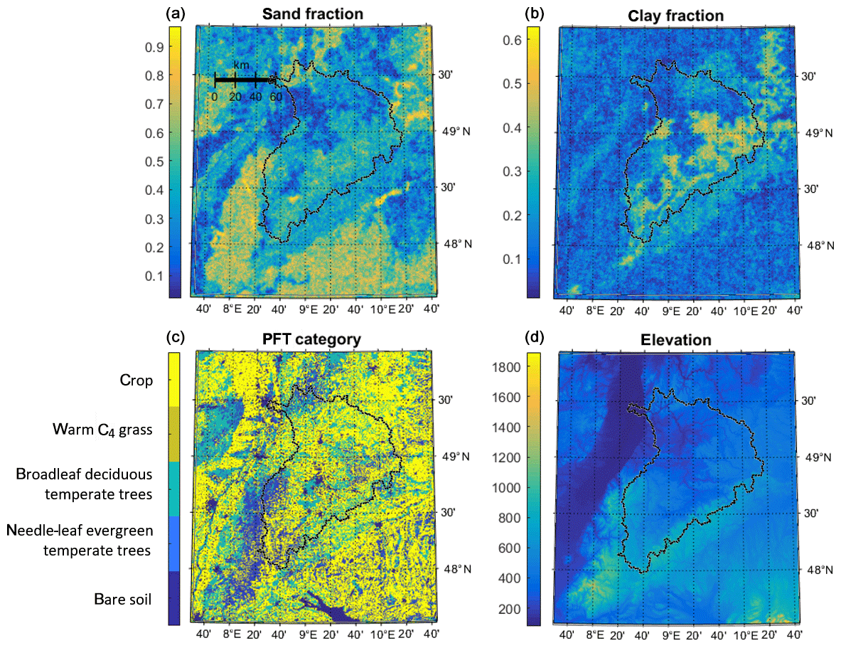
Figure 1TerrSysMP simulation area at 400 m resolution with the Neckar catchment roughly in the center indicated by the black line. Soil sand (a) and clay fractions (b) are displayed in (a, b), while the plant functional types (PTFs) used by CLM are shown in (c), and topography (in m) in (d).
The topographic data for VR01 are obtained from the European Environment Agency (EEA; http://www.eea.europa.eu/data-and-maps/data/eu-dem, last access: 11 April 2020), which is also the source for the CORINE land-use data (http://www.eea.europa.eu/data-and-maps/data/corine-land-cover-2006-raster-3, last access: 11 April 2020) used to characterize vegetation in the model domain. Since CORINE uses many more land-use classes than CLM, the CORINE classes are aggregated to the five classes discriminated in the CLM in the modeling area: broadleaf forests which can be found mostly in hilly areas throughout the domain in smaller patches, needle-leaf forests which dominate at a higher elevation such as the Black Forest, grassland which is relatively rare and only appears in small patches, and crops which are the most dominant land-use type throughout the domain and appear almost anywhere. All other classes, such as urban areas, are treated as bare soil in VR01.
The leaf area index (LAI) for the specific plant classes is taken from MODIS estimates corrected for known biases (Tian et al., 2004). Instead of the tiling approach implemented in CLM, the dominant land-use type for each grid cell is used, because the resolution of 400 m is high enough to warrant this approach. The SAI (stem area index) is estimated from the LAI by formulations slightly modified from those implemented in the CLM. For crops, SAI is just 10 % of the LAI; thus, SAI is larger in summer than in winter. For all other types, SAI is 10 % of LAI plus a “dead leaf” component. The “dead leaf” component is estimated empirically from the change of the LAI from the previous and current month. The “dead leaf” component is only a major contributor during fall, but even there the needle-leaf trees, for instance, show only a small increase in SAI. The VR01 region is mostly covered by deciduous trees that have 1–2 months of high SAI because the dead-leaf component decays rather quickly. Details about SAI calculation in VR01 are described in Schalge et al. (2016), Lawrence and Chase (2007), and Zeng et al. (2002).
The soil map (Fig. 1a–b) is derived from a product of the German Federal Institute for Geosciences and Natural Resources (BGR; https://www.bgr.bund.de/DE/Themen/Boden/Informationsgrundlagen/Bodenkundliche_Karten_Datenbanken/BUEK1000/Nutz_BUEK/nutz_buek_node.html, last access: 11 April 2020). Soil values for regions near the edge of the modeling domain in France and Switzerland are extrapolated. Variability was added to the relatively large polygons of constant soil parameters to better represent what would be found in reality at higher resolutions, following Baroni et al. (2017). The soil color is derived from the carbon content of the soil, with carbon-rich soils being darker, except for the bare soil areas, which all use the same relatively light color class. There is deep soil geology included in ParFlow as well as alluvial channels below rivers to account for deeper subsurface flow, but these features will not directly impact the results shown here as they only appear below the soil layers.
2.2 Generation of L-band passive microwave observations
The radiative transfer model CMEM (de Rosnay et al., 2009) computes the land emissivity based on a dielectric mixture model for soil moisture, soil sand and clay fractions, soil surface roughness, vegetation optical thickness, single scattering albedo, and land surface orientation relative to the satellite viewing perspective. Depending on the sand and clay fractions, brightness temperatures may vary by tens of Kelvins, given the same near-surface soil moisture. Vegetation optical thickness depends on LAI, which varies in the VR01 with time depending on plant functional type (PFT). Depending on the particular PFT, CMEM uses different parameters to calculate the vegetation optical thickness from the respective LAI. Soil effective temperature is computed with a new scheme introduced by Lv et al. (2014). The new scheme is a discretization of the integral formulation and takes advantage of multi-layer soil temperature and moisture profile information with a broader range of soil properties. This allows better adaptation of CMEM to the available land surface model data. Also, soil temperature and snow depth impact the simulated brightness temperatures. More details can be found in the SMOS global surface emission model handbook (de Rosnay et al., 2009).
From the 400 m resolution brightness temperatures, virtual satellite observations are generated with CMEM, taking the satellite antenna function into account. Figure 2 shows the centers of the ∼320 footprints corresponding to the SMOS L1 TB data product at a 41∘ incidence angle for a potential satellite overpass and – on the same scale – the satellite antenna function for one footprint, which changes shape depending on the elevation of the individual 400 m model grid areas, orbit altitude, declination, satellite scanning and incidence angle.
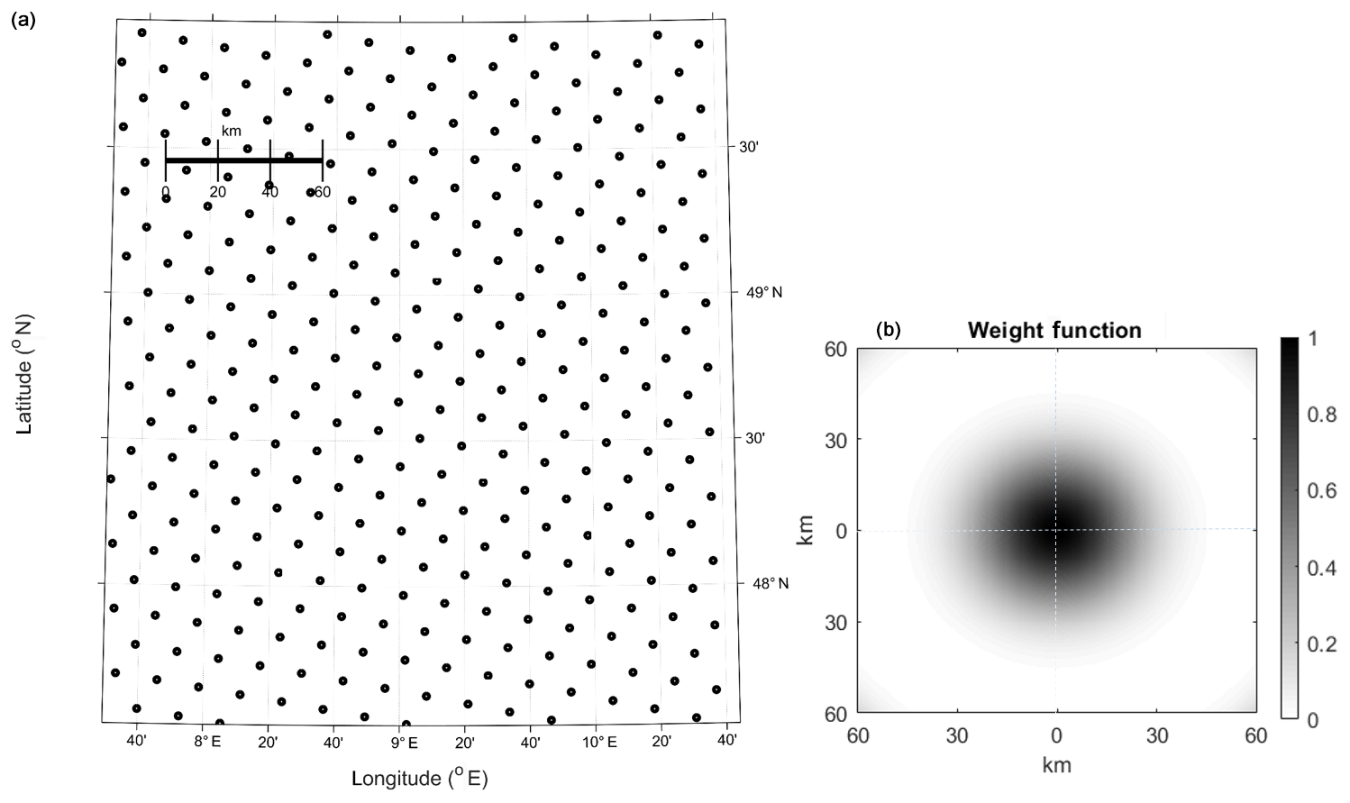
Figure 2Dots in (a) indicate the centers of SMOS footprints for one hypothetical satellite overpass, and (b) shows the antenna pattern of one satellite footprint at nadir on the same scale as the map in (a).
Not each SMOS overflight will cover the whole area in reality. But in our study, we assume for simplicity that all footprints indicated in Fig. 2 are observed once a day at 06:00 local time, which corresponds to the approximate ascending and descending overpass time of SMOS and SMAP, respectively. The satellite footprint is much larger than the nominal satellite spatial resolution of 40 km that is defined by a 3 dB contour of the main lobe; thus areas much larger in diameter contribute to one satellite-observed brightness temperature (i.e., 50 % of one satellite-observed brightness temperature originates from an area roughly 10 times larger than the nominal satellite footprint).
The virtual reality employed in this study is a physically consistent state of the terrestrial system in space and time because it has been produced by a numerical model based on the conservations equations for mass, energy, and momentum. When applying the satellite observation operator to this model state, we assume that the model state is correct, as well as the simulated brightness temperature. Thus, our study only quantifies the impact of the sampling density of a surface network on the comparison between area-averaged values and their estimates from the surface network, i.e., we ignore errors of the dynamic model (TerrSysMP) and the forward operator (CMEM). Based on the modeling results, we analyze a range of ground-based network configurations with sampling points at least 400 m apart, and we assume that all quantities (state of the terrestrial system and brightness temperature) do not vary within 400 m. While this is an approximation, we believe that our results and their outcome can be generalized. We will come back to this point in the discussion section.
Since one SMOS and SMAP footprint covers approximately 106×106 model grid columns in the VR01, the respective area can be sampled up to a maximum of 106×106 (virtual) sites. If the footprint area is sampled with n sites, there are sampling combinations (SCs, hereafter) possible, with
which is an unordered, non-overlapping collection of distinct elements of a prescribed size taken from a given set. For example, with a 10 km distance between sampling sites, about 6×6 sampling sites are possible within one footprint, which can be spatially distributed in ways. It is computationally not feasible to consider all those combinations. When, however, we first divide each footprint into equally sized subareas each containing exactly one sampling site (this assumes a certain degree of homogeneity within the network, which would in reality also be strived for), the number of potential sampling networks is drastically reduced. If we set the sampling distance within a 43×43 km2 area to i km, we divide the footprint into subareas each containing 400 m-resolution model columns. When we further select within each of the equally sized subareas of a satellite footprint the same model column (i.e., the one with row number k and column number l, both starting at 1 in the upper left column of each subarea), a regular equidistant observation network within the SMOS–SMAP footprints is enforced similar to the one used in the study by Famiglietti et al. (2008). For each footprint (subscript f) at a particular time (subscript t) of a certain sampling distance (i km, subscript d), the number of network configurations SCftd is
This results for a certain sampling distance (i km) for all 320 footprints and all 365 d of a year to a sample size of
from which we will compute the PDF of the resulting sampling errors. For each day, given one observation per day for all 320 footprints and summed over all sampling distances, we get samples of size
from which we will compute PDFs of the maximum allowed sampling distances. For each grid cell with one observation per day taken over 1 year and summed over all sampling distances, we get
from which we determine the spatial distribution of the maximum allowed sampling distances. For example, for 800 m sampling distance, we determine the maximum from samples, the number of which increases with the square of the sampling distance.
The sampling described above is applied to soil moisture (brightness temperature) with (without) considering the satellite weighting function (Fig. 2b). Since SMAP Cal/Val requires that the nominal accuracy of 0.04 cm3 cm−3 for retrievals should meet with a probability of 70 %, we take the error at the 70th percentile, if not specified otherwise. In the following, we mostly use the more intuitive sampling distance (km), but also the sampling density (sites per square kilometer) when we are qualifying tendencies. The relationship between the sampling distance and the sampling density is simply
For example, the 15, 5, and 3 sites for grid cells with diameters of 36, 9, and 3 km recommended by SMAP Cal/Val would be around 0.0116, 0.0617, and 0.3333 sites per square kilometer and correspond to sampling distances of 9.295, 4.025, and 1.732 km, respectively. We note here that the grid size of the SMAP passive soil moisture product is 36 km ×36 km per pixel, which is the ISEA-4H9 discrete global grid for SMOS (43 km ×43 km). The 43 km in all equations shall be exchanged by 36 km when computing the number of sampling networks by Eqs. (1) to (3).
We first discuss in detail the results for soil moisture sampling. Then we extend the same methodology to brightness temperature and compare both results. We also evaluate the potential sampling error for “footprints” with grid sizes of 3 and 9 km, because the SMAP products also include combined active–passive soil moisture retrievals at higher spatial resolutions (e.g., EASE-grid 9 km) and a product only based on the active sensor (EASE-grid 3 km). Two kinds of percentages are used in this study. One is the confidence level, which is related to the number of potential network configurations for one footprint as given by Eq. (2). The other percentage is related to the PDF of the maximum allowed sampling distance with a confidence level of 70 % (we also use 100 % for comparison), which is based on Eqs. (3), (4), and (5). The site numbers defined by SMAP are equivalent to the latter.
3.1 Soil moisture
We compare the true (but virtual) spatial arithmetic average of soil moisture at the SMOS–SMAP resolution with the arithmetic average of soil moisture at 0.05 m depth computed from the sampling points taken at distances ranging from 400 m (i.e., each VR01 grid column, no sampling error) to 18 km (about half the radius of a SMAP or SMOS pixel. First, we analyze the probability density function of the sampling error as it varies with the sampling distance, taking the SCft samples for one whole year of all footprints in the entire model area into account (Eq. 3, Figs. 3 and 6). Then we analyze the evolution over the year of the daily PDF of the maximum allowed sampling distance (for keeping the sampling error below the nominal value of 0.04 cm3 cm−3 with 70 % confidence) from SCtd samples (Eq. 4, Figs. 4 and 7). Finally, we look at the spatial variability of the maximum allowed sampling distance (for keeping the sampling error below the nominal value of 0.04 cm3 cm−3 with 70 % confidence) based on all samples of one SMOS–SMAP pixel over the year SCfd (Eq. 5, Figs. 5 and 8). When we analyze the sampling errors for brightness temperatures, we use footprint averages weighted by the antenna function; using the weighting function according to the dB pattern for soil moisture leads to differences below 0.01 cm3 cm−3; thus, the averaging procedure does not impact our conclusions for soil moisture.
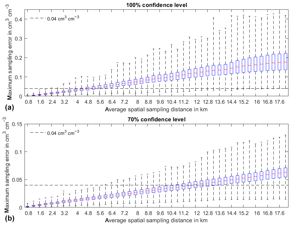
Figure 3Box–whisker plots, with the median in red, 25th and 75th percentiles as bounds of the box, and whiskers encompassing all values of the maximum sampling errors for the 320 satellite footprints of the arithmetic mean soil moisture estimated for all network configurations observing twice a day over 1 year at the given sampling distances (abscissa). Panel (a) shows the absolute maximum error, while (b) displays the results for the 70th percentile of the sampling error distribution at each satellite footprint. The horizontal dashed line is the 0.04 cm3 cm−3 retrieval error anticipated for SMOS and SMAP.
We compute the maximum sampling error for each sampling distance and each footprint from the daily observations over 1 year of all network configurations. The distributions of the corresponding 320 values are displayed in the box–whisker plots in Fig. 3a. Thus each value entering the distribution at a given sampling distance (individual box-whisker plot in Fig. 3) stems from that sampling network for one of the 320 SMOS footprints, which leads to the largest sampling error, taking all daily observations over a year into account (Eq. 3). With a sampling distance of 400 m, we accurately reproduce the true (but virtual) arithmetic soil moisture average, i.e., the maximum error is zero. Maximum errors naturally increase with sampling distance, as demonstrated by the widening of the maximum error distribution. The median of the maximum sampling error increases almost linearly, with about 0.022 cm3 cm−3 per kilometer increase in sampling distance. The spread of the maximum error increases from less than 0.01 cm3 cm−3 at 0.8 km to approximately 0.4 cm3 cm−3 at 18 km, with quite some variability between the sampling steps. To guarantee a sampling error below 0.04 cm3 cm−3 (the assumed accuracy of SMOS–SMAP retrievals) with 100 % confidence everywhere in the region at any time of the year (Fig. 3a), the maximum sampling distance should not exceed 2.8 km. With a 4.8 km sampling distance, for 50 % of the area and/or days of the year, we get sampling errors above 0.04 cm3 cm−3. At a sampling distance of 4.4 km (about 18 sites within a 43 km ×43 km pixel); the same would hold for only 25 % of the satellite pixels.
Figure 3c displays the PDF of the maximum sampling error corresponding to the 70th percentile of the sampling error PDF computed for each satellite pixel over the year. Thus, to guarantee a sampling error below 0.04 cm3 cm−3 for all network configurations for only up to 70 % of all pixels and all days of the year, a minimum sampling distance of 6 km is required. At a sampling distance of 12 km, already only 50 % of the pixels fulfill this requirement. Overall, about one-quarter of the stations needed for 100 % confidence is needed, when the requirement to stay within the 0.04 cm3 cm−3 error margin is relaxed to 70 %.
As outlined above, we can also quantify from the simulations the allowed maximum sampling distance on a daily basis from the samples with the size given by Eq. (4). According to Fig. 4b, for 80 % of the SMOS–SMAP pixels, the maximum allowed sampling distance is between 8.4 and 16 km, which is 7–26 stations for SMOS (43 km) and 5–18 stations for SMAP passive (36 km) to keep the sampling error below 0.04 cm3 cm−3 with 70 % confidence. A seasonal variation is not apparent, but rainfall events (Fig. 4a) affect the distributions by increasing the maximum allowed sampling distances because the surface soil moisture becomes more homogeneously distributed in space due to the typically quite widespread precipitation in that region. The opposite occurs during dry periods because evaporation, draining, and runoff over various soil and land cover types tend to create spatially heterogeneous soil moisture distributions, which typically reaches its maximum at intermediate soil moisture levels (Brocca et al., 2010).
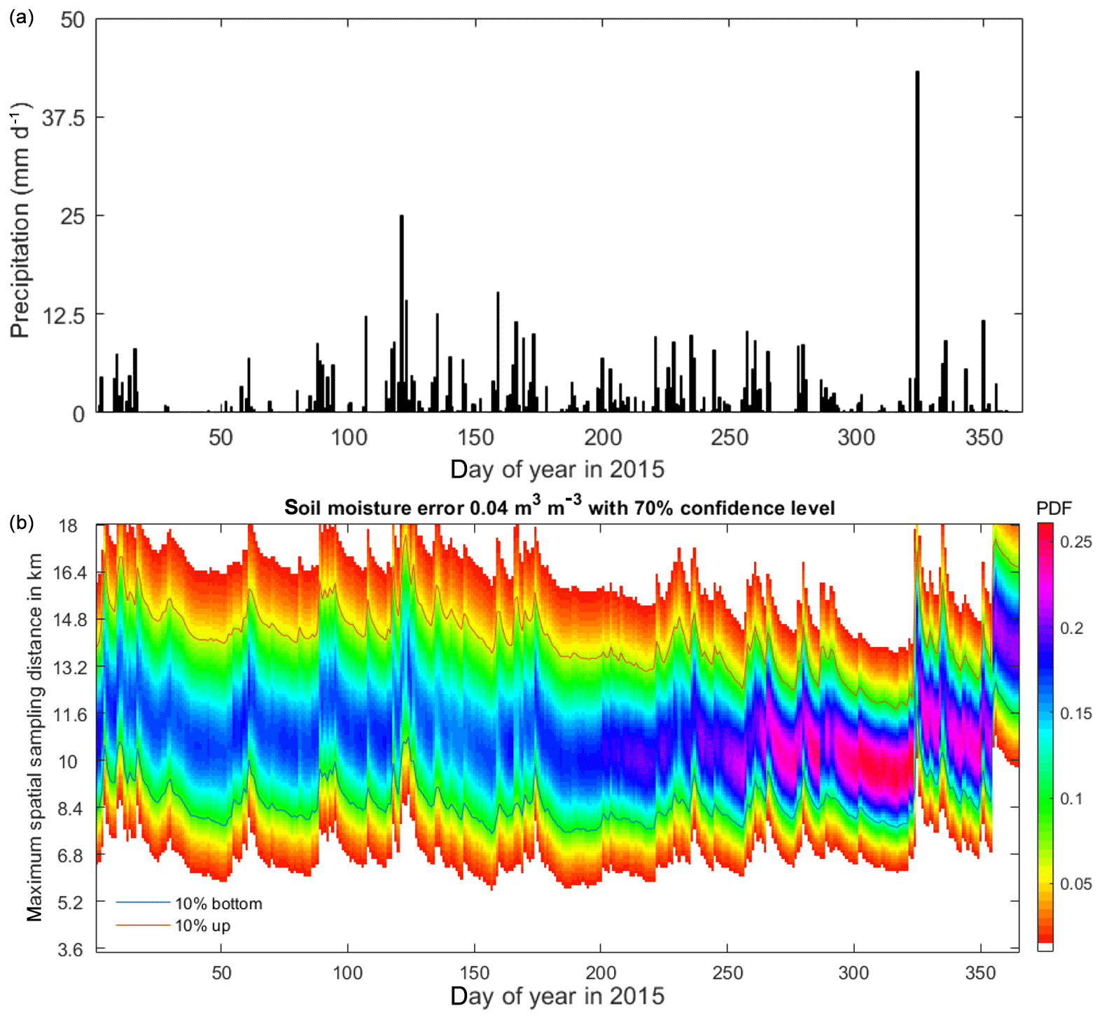
Figure 4Precipitation in VR01 (a) and time series of the distribution of the maximum allowed soil moisture sampling distance for each SMOS or SMAP pixel to assure a sampling error below 0.04 cm3 cm−3 (70 % confidence) for the year 2015 (b). The colored intensity is proportional to the probability of occurrence. The 10th and 90th percentiles are indicated as blue and read lines, respectively. Every precipitation event makes the soil moisture field more homogenous regarding high PDF and larger maximum spatial sampling distance, which means fewer stations are required.
The spatial distribution of the annual maximum sampling distance allowed to guarantee a sampling error below 0.04 cm3 cm−3 with 70 % confidence computed from the samples given by Eq. (5) and its RMS for the year 2015 (Fig. 5) indicates that the southeastern region requires sampling distances of only below 16 km; thus only nine sites are needed within a SMOS–SMAP pixel to estimate the footprint-averaged soil moisture with a sampling error below 0.04 cm3 cm−3. Also, the annual variation is particularly small (blue). For the rest of the region, maximum allowed sampling distances range from 7 to 10 km (radius); thus, more than nine sites are required within one footprint. The annual variation of the maximum sampling distances for those footprints is larger than in the southeast. The mean allowed sampling distances and their day-to-day changes are only weakly correlated (correlation coefficient 0.40), but show larger-scale common patterns.
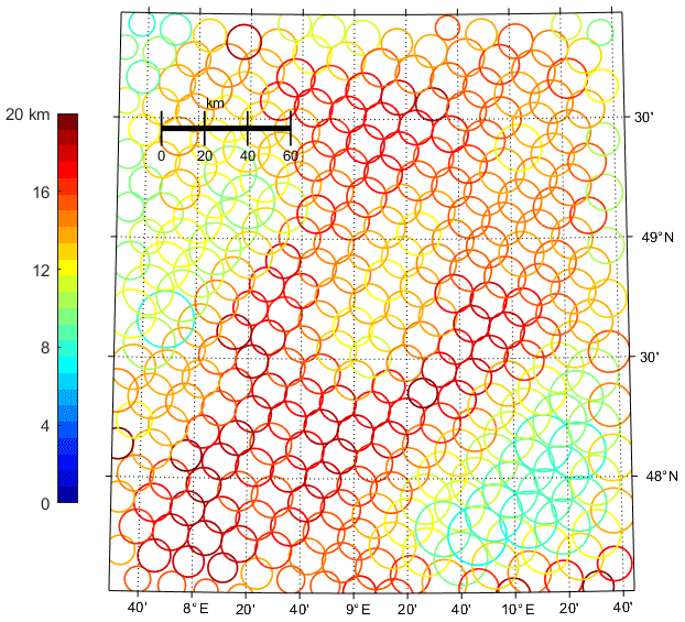
Figure 5Spatial distribution of the mean of the maximum allowed soil moisture sampling distance in the model area required for keeping the maximum sampling error below 0.04 cm3 cm−3 over the whole year. The circle radius indicates the maximum allowed sampling distance in the scale shown in the map, while its color (see color bar) gives the RMS of the maximum allowed sampling distance over time for the year 2015.
3.2 Brightness temperature
We now determine the maximum sampling distances for networks of ground-based microwave radiometers allowed to estimate SMOS–SMAP footprint brightness temperatures. To this goal, we transform the target accuracy of SMOS–SMAP soil moisture retrievals of 0.04 cm3 cm−3 to the accuracy of the corresponding brightness temperature, which is approximately 10 K for H polarization and 5 K for V polarization (10 K/5 K) according to CMEM forward simulations (Sabater et al., 2011; Monerris Belda, 2009). We note that this brightness temperature accuracy is not the instrument observing error of the (virtual) microwave radiometer, but the sensitivity of the microwave forward transfer model to soil moisture. We are aware that the radiometric accuracies of ground-based and satellite-borne sensors are much better, and that the accuracy of the soil-moisture–brightness temperature relation is mainly responsible for the retrieval accuracy; thus, we use the 10 K/5 K uncertainty only as a proxy for the overall error.
By comparing the high-res TB for certain sampling distances with the antenna pattern TB from the satellite operator, Fig. 6 shows different patterns to the soil moisture. Even at a sampling distance of 800 m, the sampling error might exceed the 10 K for H polarization (5 K for V polarization) limit in certain regions and times. If we want to keep the limit with a probability of only 75 percentiles (the upper boundary of the boxes in Fig. 6, 100 % confidence panels), the maximum sampling distance must stay below 4.4 km. For a sampling distance of 5.2 km, the error may go beyond the nominal 10 K (5 K) with a probability of 50 %. For 9.2 km sampling distance, and the maximum sampling error is always above the nominal values for some region and/or a day in the year. Even if we require that the nominal error is undercut only with a probability of 70 % for all pixels and days, a sampling distance of 800 m is not enough. If only 50 % of all networks are required to fulfill the 10 K/(5 K) bound, a sampling distance of 10 km is sufficient.

Figure 6Same as Fig. 3 but for the sampling error of the brightness temperature. The respective brightness temperature errors are (equivalent to a soil moisture accuracy of 0.04 cm3 cm−3) 10 K for H polarization and 5 K for V polarization and are indicated as dashed horizontal lines.
The time series of the distribution of the maximum sampling distances for brightness temperature (Fig. 7) is quite similar to the one for the maximum sampling distances for soil moisture. Figure 7 only illustrates the periods without freeze–thaw state transformations, and liquid water in the soil dominates the brightness temperature signal. Values range from 6.8 to 16.4 km for most cases. The spread of the sampling error has, however, a distinct seasonal variation; e.g., the maximum sampling distance for 90 % of the footprints is 11.6 km from DOY 100 to 275 and 8.8 km for the rest of the year.
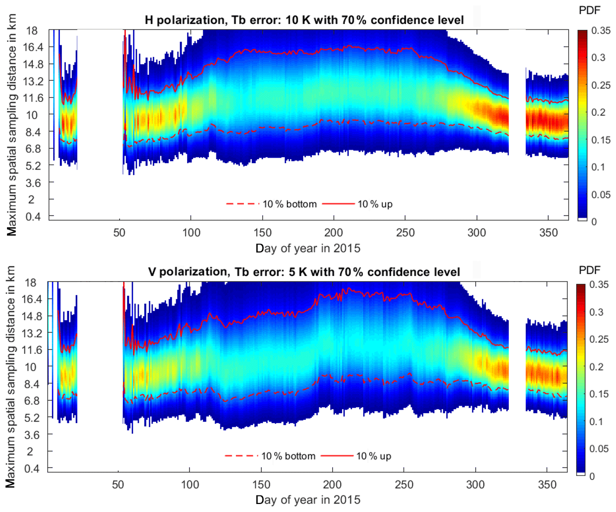
Figure 7Time series of the distribution of maximum sampling distances (70 % confidence in 10 K/5 K for H∕V polarization) for brightness temperature at every sites in 2015. The color indicates the probability of occurrence.
The spatial distribution of the annual maximum sampling distance allowed to guarantee a sampling error less than 10 K/5 K for H∕V polarized brightness temperatures, and its RMS for the year 2015 (Fig. 8) are similar for H and V polarizations but shows a substantial spatial contrast compared to the results for soil moisture (Fig. 5). Again, the southeast corner of the model region allows for larger maximum sampling distances, but there are now also other distinct regions with larger allowed maximum sampling distances. Additional input parameters required – especially LAI – and internal parameters in CMEM impact the representativeness of sites for brightness temperatures. LAI dominates the variation of the representativeness of ground-based observations and also its temporal variation, as can be inferred from the correlation between large maximum sampling distances with its variability over the year (correlation coefficient is 0.84∕0.83 for H∕V polarization), which is not observed for soil moisture. LAI is the only input in CMEM, which can lead to such a temporal variation because other parameters such as air temperature, soil moisture, and soil properties are either fixed or do not impact the brightness temperature as strongly.
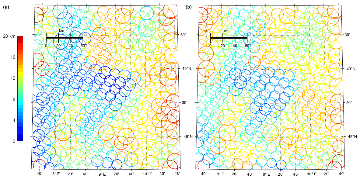
Figure 8Spatial distribution of the maximum distances of stations (diameter of circles, see scale) for surface-based brightness temperature observations required to keep the sampling error below 10 K for H polarization (a) and 5 K for V polarization (b). The color of the circles (see color bar) gives the RMS of the maximum sampling distance over time for the year 2015.
3.3 Maximum sampling distance differences between soil moisture and brightness temperature
The differences in the variability of the maximum allowed sampling distance for soil moisture and brightness temperature can be explained by using the microwave transfer model CMEM. The relationship between soil moisture and brightness temperature is complex and non-unique (Fig. 9a, b). For example, a soil moisture value of 0.4 cm3 cm−3 relates to brightness temperatures from 180 to 250 K for H polarization and 225 to 265 K for V polarization due to the variation of vegetation cover, soil properties, and terrain.
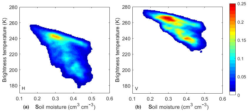
Figure 9Scatter plots of the joint PDF between brightness temperature at H (a) and V (b) polarization against soil moisture computed from the 400 m resolution virtual reality for 1 year. Both the temporal and spatial variation is included.
As already mentioned in the introduction, the spatial resolution for the SMAP active product is 3 km and for the passive–active merged soil moisture product 9 km. SMAP CAL/VAL requires three stations for the evaluation of the prior and five stations for the following product (Colliander et al., 2017b). We computed the station distance required to keep the sampling error below the nominal 0.04 cm3 cm−3 for both products by using the same methodology used above. Due to limited computation capacity, only the higher-resolution pixels in the center of the 43 km SMOS footprints are evaluated. According to the results (Fig. 10), the probability that 3 and 9 km pixels sampled with 3 and 5 stations, respectively, have sampling errors below the nominal value of 0.04 cm3 cm−3 is below 40 % and thus much lower than the required 70 %. The temporal variation of the confidence level is larger for the 3 km than for the 9 km grid size.
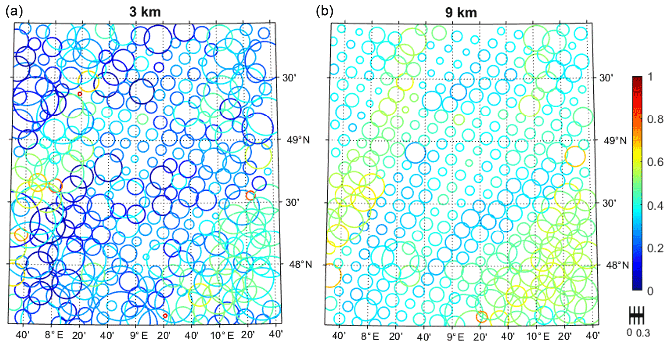
Figure 10The spatial distribution of the soil moisture sampling confidence to achieve the 0.04 cm3 cm−3 accuracy requirement by sampling 3 km (a) and 9 km footprints (b) with three and five sites, respectively (see the scale below the color bar). The colors show the minimum confidence level throughout the year 2015 for every footprint. The scale is soil moisture accuracy that can be achieved.
3.4 The impact of land surface inhomogeneity
Areas with vegetation water content above 5 kg m−2 (mostly forests) are flagged in SMAP retrievals. The networks used in the studies by Colliander et al. (2017b) and Famiglietti et al. (2008) were selected because of their relative homogeneity; thus, forested patches, open water, permanent ice and snow, urban areas, and wetlands are excluded. Soil moisture maps from SMAP/SMOS are, however, global. Thus estimates are provided everywhere, and signals from open water surfaces on subgrid scales may influence the products. We used our simulated observations to study the impact of subpixel contributions of forested areas on the sampling errors.
In total, only 16 of the 320 footprints covering the model area have forest fractions below 15 % and negligible surface water contributions; such footprints are usually considered ideal for soil moisture Cal/Val. In terms of both soil moisture and brightness temperature, their maximum sampling errors are considerably lower compared to all sites for all sampling distances (Fig. 11). Thus, excluding sites with larger forest fractions leads to lower sampling errors.
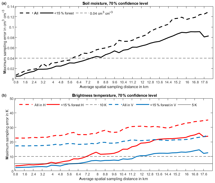
Figure 11The maximum sampling errors of the arithmetic mean of soil moisture (a) and brightness temperature (b) estimated from all sites and from sites with forest cover below 15 % against average sampling distance.
The results shown in Fig. 11 do not mean that forest sites always have higher soil moisture errors than non-forest sites, but by picking Cal/Val sites with favorable conditions reduces the required sampling density, which may, however, affect their representativeness. Moreover, the required sampling density inferred from non-forest sites cannot be extended to forest sites.
We used a virtual reality generated with a fully coupled subsurface–vegetation–atmosphere model platform over southwestern Germany with a spatial resolution of 400 m for the land components to quantify the sampling error for the arithmetic averaged soil moisture and the weighted average brightness temperatures estimated from in situ ground-based observation networks covering SMOS–SMAP-like footprints of 43 km diameter for a wide range of potential sampling distances. By using a virtual reality at such high resolution, we have a physically consistent three-dimensional evolution of the terrestrial system at our disposal from which we can take virtual soil moisture observations and – via the radiative transfer model CMEM and a satellite antenna function – microwave brightness temperature observations from the highest resolution at 400 m to any larger resolution.
As an upper threshold for the sampling error of ground-based sensor networks when estimating averages over SMOS–SMAP pixels, we adopted the target SMOS–SMAP soil moisture retrieval accuracy of 0.04 cm3 cm−3. We quantified the maximum sampling distance, which still keeps the sampling error below that accuracy either for all or for 70 % of all SMOS–SMAP pixels in the modeling region over 1 year for all network configurations possible. A primary assumption in our study is that the estimation of soil moisture for an area with a diameter of about 400 m is possible, or in other words that a single station within a 400 m area is representative for its spatial average, an assumption also discussed in Famiglietti et al. (2008). Compared to the region analyzed in Famiglietti et al. (2008), our study uses a much more realistic terrain and excludes subjective factors in selecting suitable Cal/Val sites. Because of this, the soil moisture error in our study grows much faster with increasing sampling distance. We also find that the estimation of area-averaged brightness temperatures from a network of ground-based stations has a different error growth with increasing sampling distance compared to soil moisture despite an initial linear growth for both of them (compare Figs. 3 and 6). Thus, a representative soil moisture network does not guarantee a representative radiometer network for the estimation of area-averaged brightness temperature, or that brightness temperatures computed for the soil moisture stations can be used for that estimate. But Figs. 3 and 6 also show that sampling distances below 6 km still fulfill the 70th percentage requirement for keeping the sampling error below the nominal error.
Besides plant types, there is no apparent pattern similarity between clay, sand, and elevation (Fig. 1) and spatial sampling distance (Fig. 5). Soil properties may be related to the regional climate (annual precipitation, radiation flux balance, etc.). For instance, arid regions usually contain higher sand fractions, but such areas are seldom the focus of soil moisture studies because of their low variation. Transition zones like our model area usually encompass various soil properties, which are often correlated with land use and vegetation and thus the plant function type used in the CLM. Topography also affects the soil moisture and TB distribution, but it is difficult to infer the impact of land use and vegetation because soil properties determine both the water holding capacity and the plant cover. In practice, soil moisture monitoring networks avoid complex terrain. Homogenous terrain and landscape lead to an overestimation of satellite soil moisture product accuracies.
The statistical results in our study differ from those in Famiglietti et al. (2008) because our focus is on the satellite footprint scale and not the representativeness of one station within a network. For example, a particular sensor may not represent the actual 400 m average, but one such sensor every 400 m may statistically sufficiently represent a much larger footprint. A similar concept is adapted in ensemble forecasts using members, e.g., with different physics packages, none of which is expected to be the truth (Lewis, 2005; Leutbecher and Palmer, 2008). The space detected by a soil moisture sensor, which is measuring the dielectric constant of the soil or other media using capacitance/frequency domain technology, is about a 10 cm sphere. Thus, the study by Famiglietti et al. (2008) assumes soil moisture homogeneity on the scale of meters. We believe that the 400 m soil moisture homogenous assumption does not interfere with our conclusions and that our study can be considered as a complement to the study by Famiglietti et al. (2008).
The calibration and validation of passive satellite-based L-band soil moisture estimates are difficult due to the large subpixel variability (Lv et al., 2016b, 2019). Even with a perfect microwave transfer model and precise sensors, we can hardly find an appropriate in situ observation to compare with. While soil moisture also varies in the vertical, sensors are usually mounted at a fixed depth; thus, comparisons with satellite observations require the knowledge of the microwave penetration depth, which is, however, unknown in general. Lv et al. (2018) developed a model based on the soil effective temperature which sheds light on this fundamental problem. This study isolates the sampling density issue from other factors and is a test of the current Cal/Val network standard without previous knowledge of the site. The SMAP team suggests 15 sites for a 36 km by 36 km grid size (Colliander et al., 2017b), and this study agrees with this configuration for typical mid-latitude European regions from the sampling error perspective. For a 36 km by 36 km grid size, the required sampling sites would range from about 36 (6 km) to 4 (17 km). However, five sites for 9 km by 9 km and three sites for 3 km by 3 km will miss the 70 % confidence level requirements over this area. Since SMAP's 9 and 3 km soil moisture products are from a combination of passive and active microwave signals, which have a lower accuracy than the passive ones (Entekhabi et al., 2010), their Cal/Val campaigns shall determine sampling distances with less confidence level.
Our virtual reality contains extensive land cover variability (Fig. 1); thus, it would be helpful to adapt our approach for less complicated regions with variabilities closer to the typical Cal/Val station networks. Overall, we find that a soil moisture sampling distance of ∼3 km is necessary to always keep the sampling errors below the nominal value. The allowance for a failure probability of 30 % extends this distance to 10 km. For brightness temperatures, the sampling requirements are much more strict; already, at 800 m sampling distance, it cannot be guaranteed that the sampling error remains below the equivalent threshold of 10 K/5 K for H and V polarization, respectively, even when allowing for a 30 % probability of failure. The error sources in retrieving soil moisture from TB data are also large in reality but are not of concern in this study because VR01 and the TB produced by CMEM exclude the uncertainty, except for the sampling distance.
Our results are not only useful for the planning of ground-based soil moisture networks, they also contribute to a better understanding of the relation between brightness temperatures observed on the ground – or simulated at high resolution – and the ones observed from satellites, apart from the non-linearity effects of radiative transfer (e.g., Drusch et al., 1999). The study allows, for example, to quantify to what extent a bias between satellites' brightness temperature and forward simulation could be explained by the spatial sampling (e.g., Figs. 5, 8, and 11), and to understand the similarities and dissimilarities between observed soil moisture and brightness temperature time-series (Figs. 4 and 7). Since ground-based soil moisture networks will always cover only certain parts of a satellite pixel, a bias must be expected between both. The different representativeness of the latter can also cause biases in satellite and ground-based estimates of soil moisture for soil moisture and brightness temperatures.
While the allowed maximum sampling distances do not change much over the year for soil moisture – except after large-scale precipitation events which will enable larger sampling distances – its equivalence for brightness temperature has a strong seasonal variation because of the blurring effect of vegetation during the growing season, when brightness temperatures become more homogeneous. The spatial distribution of the maximum sampling distances and their local variances behave quite differently between soil moisture and brightness temperature. The spatial patterns are different, and while the maximum allowed sampling distance and its variation are firmly related to brightness temperature, they are barely related to soil moisture; this unusual behavior is caused by the complexity of other factors influencing microwave radiative transfer.
Our study strongly suggests that the sampling density of current SMOS–SMAP ground-based Cal/Val networks and the resulting potential sampling error of estimated pixel-mean soil moisture and brightness temperatures considered in such studies should be reviewed carefully. We expect this study will help us to understand the errors of satellite-derived soil moisture better.
The dataset is published at https://cera-www.dkrz.de/WDCC/ui/cerasearch/q?query=neckar&page=0&rows=15 (last access: 11 April 2020). We use for this study available simulation results generated by the research unit FOR2131 (Schalge et al., 2016, 2018, 2019) over an area containing the Neckar catchment in southwestern Germany in its center (Fig. 1).
SL and CZ conceived of the presented idea. BS provided the VR01 dataset and data section. SL and PSG developed the codes and performed the computations. CZ helped supervise the project.
The authors declare that they have no conflict of interest.
Computing time was provided by the Gauss Centre for Supercomputing (http://www.gauss-centre.eu/gauss-centre/EN/Home/home_node.html, last access: 11 April 2020) operated by the Juelich Supercomputing Centre (http://www.fz-juelich.de/ias/jsc/EN/Home/home_node.html last access: 11 April 2020). We thank the members of HPSC-TerrSys (http://www.hpsc-terrsys.de/hpsc-terrsys/EN/Home/home_node.html, last access: 11 April 2020) and Klaus Goergen in particular for invaluable technical support with the JUQUEEN supercomputer. Furthermore, we thank Prabhakar Shresta and Mauro Sulis from the Transregional Collaborative Research Center 32 (TR32) for their preliminary work and introduction to the TerrSysMP modeling platform
This research was funded by the Deutsche Forschungsgemeinschaft (DFG) via FOR2131: “Data Assimilation for Improved Characterization of Fluxes across Compartmental Interfaces”, subproject P2.
This paper was edited by Pierre Gentine and reviewed by three anonymous referees.
Ashby, S. F. and Falgout, R. D.: A parallel multigrid preconditioned conjugate gradient algorithm for groundwater flow simulations, Nucl. Sci. Eng., 124, 145–159, 1996.
Baldauf, M., Seifert, A., Förstner, J., Majewski, D., Raschendorfer, M., and Reinhardt, T.: Operational convective-scale numerical weather prediction with the COSMO model: Description and sensitivities, Mon. Weather Rev., 139, 3887–3905, 2011.
Baroni, G., Zink, M., Kumar, R., Samaniego, L., and Attinger, S.: Effects of uncertainty in soil properties on simulated hydrological states and fluxes at different spatio-temporal scales, Hydrol. Earth Syst. Sci., 21, 2301–2320, https://doi.org/10.5194/hess-21-2301-2017, 2017.
Bhuiyan, H. A. K. M., McNairn, H., Powers, J., Friesen, M., Pacheco, A., Jackson, T. J., Cosh, M. H., Colliander, A., Berg, A., Rowlandson, T., Bullock, P., and Magagi, R.: Assessing SMAP Soil Moisture Scaling and Retrieval in the Carman (Canada) Study Site, Vadose Zone J., 17, 180132, https://doi.org/10.2136/vzj2018.07.0132, 2018.
Brocca, L., Melone, F., Moramarco, T., and Morbidelli, R.: Spatial-temporal variability of soil moisture and its estimation across scales, Water Resour. Res., 46, W02516, https://doi.org/10.1029/2009wr008016, 2010.
Burgin, M. S., Colliander, A., Njoku, E. G., Chan, S. K., Cabot, F., Kerr, Y. H., Bindlish, R., Jackson, T. J., Entekhabi, D., and Yueh, S. H.: A Comparative Study of the SMAP Passive Soil Moisture Product With Existing Satellite-Based Soil Moisture Products, IEEE T. Geosci. Remote, 55, 2959–2971, https://doi.org/10.1109/Tgrs.2017.2656859, 2017.
Chen, F., Crow, W. T., Colliander, A., Cosh, M. H., Jackson, T. J., Bindlish, R., Reichle, R. H., Chan, S. K., Bosch, D. D., Starks, P. J., Goodrich, D. C., and Seyfried, M. S.: Application of Triple Collocation in Ground-Based Validation of Soil Moisture Active/Passive (SMAP) Level 2 Data Products, IEEE J. Sel. Top. Appl., 10, 489–502, https://doi.org/10.1109/Jstars.2016.2569998, 2017.
Chen, F., Crow, W. T., Bindlish, R., Colliander, A., Burgin, M. S., Asanuma, J., and Aida, K.: Global-scale evaluation of SMAP, SMOS and ASCAT soil moisture products using triple collocation, Remote Sens. Environ., 214, 1–13, https://doi.org/10.1016/j.rse.2018.05.008, 2018.
Chen, F., Crow, W. T., Cosh, M. H., Colliander, A., Asanuma, J., Berg, A., Bosch, D. D., Caldwell, T. G., Collins, C. H., and Jensen, K. H.: Uncertainty of reference pixel soil moisture averages sampled at SMAP core validation sites, J. Hydrometeorol., 20, 1553–1569, 2019.
Colliander, A., Cosh, M. H., Misra, S., Jackson, T. J., Crow, W. T., Chan, S., Bindlish, R., Chae, C., Collins, C. H., and Yueh, S. H.: Validation and scaling of soilmoisture in a semi-arid environment: SMAP validation experiment 2015 (SMAPVEX15), Remote Sens. Environ., 196, 101–112, https://doi.org/10.1016/j.rse.2017.04.022, 2017a.
Colliander, A., Jackson, T. J., Bindlish, R., Chan, S., Das, N., Kim, S. B., Cosh, M. H., Dunbar, R. S., Dang, L., Pashaian, L., Asanuma, J., Aida, K., Berg, A., Rowlandson, T., Bosch, D., Caldwell, T., Caylor, K., Goodrich, D., al Jassar, H., Lopez-Baeza, E., Martínez-Fernández, J., González-Zamora, A., Livingston, S., McNairn, H., Pacheco, A., Moghaddam, M., Montzka, C., Notarnicola, C., Niedrist, G., Pellarin, T., Prueger, J., Pulliainen, J., Rautiainen, K., Ramos, J., Seyfried, M., Starks, P., Su, Z., Zeng, Y., van der Velde, R., Thibeault, M., Dorigo, W., Vreugdenhil, M., Walker, J. P., Wu, X., Monerris, A., O'Neill, P. E., Entekhabi, D., Njoku, E. G., and Yueh, S.: Validation of SMAP surface soil moisture products with core validation sites, Remote Sens. Environ., 191, 215–231, https://doi.org/10.1016/j.rse.2017.01.021, 2017b.
Coopersmith, E. J., Cosh, M. H., Bell, J. E., Kelly, V., Hall, M., Palecki, M. A., and Temimi, M.: Deploying temporary networks for upscaling of sparse network stations, Int. J. Appl. Earth Obs., 52, 433–444, https://doi.org/10.1016/j.jag.2016.07.013, 2016.
Cosh, M. H., Jackson, T. J., Starks, P., Bosch, D., Collins, C. H., Seyfried, M., Prueger, J., Livingston, S., and Bindlish, R.: Strategies for validating satellite soil moisture products using in situ networks: Lessons from the USDA-ARS watersheds, 2017 IEEE International Geoscience and Remote Sensing Symposium (IGARSS), Fort Worth, TX, 2017, 2015–2018, available at: https://ieeexplore.ieee.org/abstract/document/8127377 (last access: 15 April 2020), 2017.
Crow, W. T., Berg, A. A., Cosh, M. H., Loew, A., Mohanty, B. P., Panciera, R., de Rosnay, P., Ryu, D., and Walker, J. P.: Upscaling Sparse Ground‐Based Soil Moisture Observations for The Validation of Coarse‐Resolution Satellite Soil Moisture Products, Rev. Geophys., 50, RG2002, https://doi.org/10.1029/2011RG000372, 2012.
dall'Amico, J. T., Schlenz, F., Loew, A., and Mauser, W.: First Results of SMOS Soil Moisture Validation in the Upper Danube Catchment, IEEE T. Geosci. Remote, 50, 1507–1516, https://doi.org/10.1109/Tgrs.2011.2171496, 2012.
Delwart, S., Bouzinac, C., Wursteisen, P., Berger, M., Drinkwater, M., Martin-Neira, M., and Kerr, Y. H.: SMOS validation and the COSMOS campaigns, IEEE T. Geosci. Remote, 46, 695–704, 2008.
de Rosnay, P., Calvet, J. C., Kerr, Y., Wigneron, J. P., Lemaitre, F., Escorihuela, M. J., Sabater, J. M., Saleh, K., Barrie, J. L., Bouhours, G., Coret, L., Cherel, G., Dedieu, G., Durbe, R., Fntz, N. E. D., Froissard, F., Hoedjes, J., Kruszewski, A., Lavenu, F., Suquia, D., and Waldteufel, P.: SMOSREX: A long term field campaign experiment for soil moisture and land surface processes remote sensing, Remote Sens. Environ., 102, 377–389, https://doi.org/10.1016/j.rse.2006.02.021, 2006.
de Rosnay, P., Drusch, M., and Munoz-Sabater, J.: Milestone 1 Technical Note Part I: SMOS global surface emission model. Technical report, European Centre for Medium-Range Weather Forecast, Reading, United Kingdom, available at: https://www.ecmwf.int/sites/default/files/elibrary/2014/18219-smos-monitoring-report-number-iv.pdf (last access: 15 April 2020), 2009.
Dorigo, W. A., Wagner, W., Hohensinn, R., Hahn, S., Paulik, C., Xaver, A., Gruber, A., Drusch, M., Mecklenburg, S., van Oevelen, P., Robock, A., and Jackson, T.: The International Soil Moisture Network: a data hosting facility for global in situ soil moisture measurements, Hydrol. Earth Syst. Sci., 15, 1675–1698, https://doi.org/10.5194/hess-15-1675-2011, 2011.
Drusch, M., Wood, E. F., and Simmer, C.: Up-scaling effects in passive microwave remote sensing: ESTAR 1.4 GHz measurements during SGP '97, Geophys. Res. Lett., 26, 879–882, https://doi.org/10.1029/1999gl900150, 1999.
Entekhabi, D., Njoku, E. G., O'Neill, P. E., Kellogg, K. H., Crow, W. T., Edelstein, W. N., Entin, J. K., Goodman, S. D., Jackson, T. J., Johnson, J., Kimball, J., Piepmeier, J. R., Koster, R. D., Martin, N., McDonald, K. C., Moghaddam, M., Moran, S., Reichle, R., Shi, J. C., Spencer, M. W., Thurman, S. W., Tsang, L., and Van Zyl, J.: The Soil Moisture Active Passive (SMAP) Mission, P. IEEE, 98, 704–716, https://doi.org/10.1109/jproc.2010.2043918, 2010.
Famiglietti, J. S., Ryu, D. R., Berg, A. A., Rodell, M., and Jackson, T. J.: Field observations of soil moisture variability across scales, Water Resour. Res., 44, W01423, https://doi.org/10.1029/2006wr005804, 2008.
Gasper, F., Goergen, K., Shrestha, P., Sulis, M., Rihani, J., Geimer, M., and Kollet, S.: Implementation and scaling of the fully coupled Terrestrial Systems Modeling Platform (TerrSysMP v1.0) in a massively parallel supercomputing environment – a case study on JUQUEEN (IBM Blue Gene/Q), Geosci. Model Dev., 7, 2531–2543, https://doi.org/10.5194/gmd-7-2531-2014, 2014.
Jackson, T., Colliander, A., Kimball, J., Reichle, R., Crow, W., Entekhabi, D., and Neill, P.: Science data calibration and validation plan, Jet Propuls. Lab, available at: https://smap.jpl.nasa.gov/system/internal_resources/details/original/518_CalVal_Plan_Rel_A_web.pdf (last access: 15 April 2020), 2012.
Kerr, Y. H., Waldteufel, P., Wigneron, J. P., Delwart, S., Cabot, F., Boutin, J., Escorihuela, M. J., Font, J., Reul, N., Gruhier, C., Juglea, S. E., Drinkwater, M. R., Hahne, A., Martin-Neira, M., and Mecklenburg, S.: The SMOS Mission: New Tool for Monitoring Key Elements of the Global Water Cycle, P. IEEE, 98, 666–687, https://doi.org/10.1109/Jproc.2010.2043032, 2010.
Kerr, Y. H., Al-Yaari, A., Rodriguez-Fernandez, N., Parrens, M., Molero, B., Leroux, D., Bircher, S., Mahmoodi, A., Mialon, A., Richaume, P., Delwart, S., Al Bitar, A., Pellarin, T., Bindlish, R., Jackson, T. J., Rudiger, C., Waldteufel, P., Mecklenburg, S., and Wigneron, J. P.: Overview of SMOS performance in terms of global soil moisture monitoring after six years in operation, Remote Sens. Environ., 180, 40–63, https://doi.org/10.1016/j.rse.2016.02.042, 2016.
Kollet, S. J., Maxwell, R. M., Woodward, C. S., Smith, S., Vanderborght, J., Vereecken, H., and Simmer, C.: Proof of concept of regional scale hydrologic simulations at hydrologic resolution utilizing massively parallel computer resources, Water Resour. Res., 46, W04201, https://doi.org/10.1029/2009WR008730, 2010.
Lawrence, P. J. and Chase, T. N.: Representing a new MODIS consistent land surface in the Community Land Model (CLM 3.0), J. Geophys. Res.-Biogeo., 112, G01023, https://doi.org/10.1029/2006JG000168, 2007.
Leutbecher, M. and Palmer, T. N.: Ensemble forecasting, J. Comput. Phys., 227, 3515–3539, https://doi.org/10.1016/j.jcp.2007.02.014, 2008.
Lewis, J. M.: Roots of ensemble forecasting, Mon. Weather Rev., 133, 1865–1885, https://doi.org/10.1175/Mwr2949.1, 2005.
Lv, S., Wen, J., Zeng, Y., Tian, H., and Su, Z.: An improved two-layer algorithm for estimating effective soil temperature in microwave radiometry using in situ temperature and soil moisture measurements, Remote Sens. Environ., 152, 356–363, https://doi.org/10.1016/j.rse.2014.07.007, 2014.
Lv, S., Zeng, Y., Wen, J., and Su, Z.: A reappraisal of global soil effective temperature schemes, Remote Sens. Environ., 183, 144–153, https://doi.org/10.1016/j.rse.2016.05.012, 2016a.
Lv, S., Zeng, Y., Wen, J., Zheng, D., and Su, Z.: Determination of the Optimal Mounting Depth for Calculating Effective Soil Temperature at L-Band: Maqu Case, Remote Sensing, 8, 476, https://doi.org/10.3390/rs8060476, 2016b.
Lv, S., Zeng, Y., Wen, J., Zhao, H., and Su, Z.: Estimation of Penetration Depth from Soil Effective Temperature in Microwave Radiometry, Remote Sensing, 10, 519, https://doi.org/10.3390/rs10040519, 2018.
Lv, S., Zeng, Y., Su, Z., and Wen, J.: A Closed-Form Expression of Soil Temperature Sensing Depth at L-Band, IEEE T. Geosci. Remote, 57, 4889–4897, https://doi.org/10.1109/TGRS.2019.2893687, 2019.
Molero, B., Leroux, D. J., Richaume, P., Kerr, Y. H., Merlin, O., Cosh, M. H., and Bindlish, R.: Multi-Timescale Analysis of the Spatial Representativeness of In Situ Soil Moisture Data within Satellite Footprints, J. Geophys. Res.-Atmos., 123, 3–21, https://doi.org/10.1002/2017jd027478, 2018.
Monerris Belda, A.: Experimental estimation of soil emissivity and its application to soil moisture retrieval in the SMOS Mission, Tesi doctoral, UPC, Departament de Teoria del Senyal i Comunicacions, available at: http://hdl.handle.net/2117/94257 (last access: 15 April 2020), 2009.
Montzka, C., Bogena, H. R., Weihermuller, L., Jonard, F., Bouzinac, C., Kainulainen, J., Balling, J. E., Loew, A., Dall'Amico, J. T., Rouhe, E., Vanderborght, J., and Vereecken, H.: Brightness Temperature and Soil Moisture Validation at Different Scales During the SMOS Validation Campaign in the Rur and Erft Catchments, Germany, IEEE T. Geosci. Remote, 51, 1728–1743, https://doi.org/10.1109/Tgrs.2012.2206031, 2013.
Njoku, E. G. and Kong, J.-A.: Theory for passive microwave remote-sensing of near-surface soil-moisture, J. Geophys. Res., 82, 3108–3118, 1977.
O'Neill, P., Chan, S., Njoku, E., Jackson, T., and Bindlish, R.: Soil Moisture Active Passive (SMAP), Algorithm Theoretical Basis Document, Level 2 & 3 Soil Moisture (Passive) Data Products, Revison B, 2015.
Ochsner, T. E., Cosh, M. H., Cuenca, R. H., Dorigo, W. A., Draper, C. S., Hagimoto, Y., Kerr, Y. H., Larson, K. M., Njoku, E. G., Small, E. E., and Zreda, M.: State of the Art in Large-Scale Soil Moisture Monitoring, Soil Sci. Soc. Am. J., 77, 1888–1919, https://doi.org/10.2136/sssaj2013.03.0093, 2013.
Oleson, K., Niu, G. Y., Yang, Z. L., Lawrence, D., Thornton, P., Lawrence, P., Stöckli, R., Dickinson, R., Bonan, G., and Levis, S.: Improvements to the Community Land Model and their impact on the hydrological cycle, J. Geophys. Res.-Biogeo., 113, G01021, https://doi.org/10.1029/2007JG000563, 2008.
Qin, J., Yang, K., Lu, N., Chen, Y. Y., Zhao, L., and Han, M. L.: Spatial upscaling of in-situ soil moisture measurements based on MODIS-derived apparent thermal inertia, Remote Sens. Environ., 138, 1–9, https://doi.org/10.1016/j.rse.2013.07.003, 2013.
Sabater, J. M., De Rosnay, P., and Balsamo, G.: Sensitivity of L-band NWP forward modelling to soil roughness, Int. J. Remote Sens., 32, 5607–5620, https://doi.org/10.1080/01431161.2010.507260, 2011.
Schalge, B., Rihani, J., Baroni, G., Erdal, D., Geppert, G., Haefliger, V., Haese, B., Saavedra, P., Neuweiler, I., Hendricks Franssen, H.-J., Ament, F., Attinger, S., Cirpka, O. A., Kollet, S., Kunstmann, H., Vereecken, H., and Simmer, C.: High-Resolution Virtual Catchment Simulations of the Subsurface-Land Surface-Atmosphere System, Hydrol. Earth Syst. Sci. Discuss., https://doi.org/10.5194/hess-2016-557, 2016.
Schalge, B., Baroni, G., Haese, B., Erdal, D., Geppert, G., Saavedra, P., Haefliger, V., Vereecken, H., Attinger, S., Kunstmann, H., Cirpka, O. A., Ament, F., Kollet, S., Neuweiler, I., Hendricks Franssen, H.-J., and Simmer, C.: Virtual catchment simulation based on the Neckar region version 1, https://doi.org/10.26050/WDCC/Neckar_VCS_v1, 2018.
Schalge, B., Haefliger, V., Kollet, S., and Simmer, C.: Improvement of surface run-off in the hydrological model ParFlow by a scale-consistent river parameterization, Hydrol. Process., 33, 2006–2019, https://doi.org/10.1002/hyp.13448, 2019.
Shrestha, P., Sulis, M., Masbou, M., Kollet, S., and Simmer, C.: A Scale-Consistent Terrestrial Systems Modeling Platform Based on COSMO, CLM, and ParFlow, Mon. Weather Rev., 142, 3466–3483, https://doi.org/10.1175/mwr-d-14-00029.1, 2014.
Shrestha, P., Kurtz, W., Vogel, G., Schulz, J. P., Sulis, M., Franssen, H. J. H., Kollet, S., and Simmer, C.: Connection Between Root Zone Soil Moisture and Surface Energy Flux Partitioning Using Modeling, Observations, and Data Assimilation for a Temperate Grassland Site in Germany, J. Geophys. Res.-Biogeo., 123, 2839–2862, https://doi.org/10.1029/2016jg003753, 2018a.
Shrestha, P., Sulis, M., Simmer, C., and Kollet, S.: Effects of horizontal grid resolution on evapotranspiration partitioning using TerrSysMP, J. Hydrol., 557, 910–915, https://doi.org/10.1016/j.jhydrol.2018.01.024, 2018b.
Simmer, C., Masbou, M., Thiele-Eich, I., Amelung, W., Crewell, S., Diekkrüger, B., Ewert, F., Hendricks-Franssen, H., Huisman, J. A., Kemna, A., Klitzsch, N., Kollet, S., Langensiepen, M., Löhnert, U., Rahman, A. M., Rascher, U., Schneider, K., Schween, J., Shao, Y., Shrestha, P., Stiebler, M., Sulis, M., Vanderborght, J., Vereecken, H., van der Kruk, J., Waldhoff, G., and Zerenner, T.: Monitoring and Modeling the Terrestrial System from Pores to Catchments – the Transregional Collaborative Research Center on Patterns in the Soil-Vegetation-Atmosphere System, B. Am. Meteorol. Soc., 96, 1765–1787, https://doi.org/10.1175/BAMS-D-13-00134.1, 2015.
Sulis, M., Langensiepen, M., Shrestha, P., Schickling, A., Simmer, C., and Kollet, S. J.: Evaluating the influence of plant-specific physiological parameterizations on the partitioning of land surface energy fluxes, J. Hydrometeorol., 16, 517–533, 2015.
Tian, Y., Dickinson, R., Zhou, L., Zeng, X., Dai, Y., Myneni, R., Knyazikhin, Y., Zhang, X., Friedl, M., and Yu, H.: Comparison of seasonal and spatial variations of leaf area index and fraction of absorbed photosynthetically active radiation from Moderate Resolution Imaging Spectroradiometer (MODIS) and Common Land Model, J. Geophys. Res.-Atmos., 109, D01103, https://doi.org/10.1029/2003JD003777, 2004.
Ulaby, F. T., Moore, R. K., and Fung, A. K.: Microwave Remote Sensing Active and Passive-Volume III: From Theory to Applications, Artech House, Inc, available at: https://ntrs.nasa.gov/search.jsp?R=19860041708 (last access: 15 April 2020), 1986.
Vereecken, H., Huisman, J. A., Bogena, H., Vanderborght, J., Vrugt, J. A., and Hopmans, J. W.: On the value of soil moisture measurements in vadose zone hydrology: A review, Water Resour. Res., 44, W00d06, https://doi.org/10.1029/2008wr006829, 2008.
Zeng, X., Shaikh, M., Dai, Y., Dickinson, R. E., and Myneni, R.: Coupling of the common land model to the NCAR community climate model, J. Climate, 15, 1832–1854, 2002.