Evaluation of global terrestrial evapotranspiration using state-of-the-art approaches in remote sensing, machine learning and land surface modeling

Evapotranspiration (ET) is critical in linking global water, carbon and energy cycles. However, direct measurement of global terrestrial ET is not feasible. Here, we first reviewed the basic theory and state-of-the-art approaches for estimating global terrestrial ET, including remote-sensing-based physical models, machine-learning algorithms and land surface models (LSMs). We then utilized 4 remote-sensing-based physical models, 2 machine-learning algorithms and 14 LSMs to analyze the spatial and temporal variations in global terrestrial ET. The results showed that the ensemble means of annual global terrestrial ET estimated by these three categories of approaches agreed well, with values ranging from 589.6 mm yr⁻¹ (6.56×10⁴ km³ yr⁻¹) to 617.1 mm yr⁻¹ (6.87×10⁴ km³ yr⁻¹). For the period from 1982 to 2011, both the ensembles of remote-sensing-based physical models and machine-learning algorithms suggested increasing trends in global terrestrial ET (0.62 mm yr⁻² with a significance level of p<0.05 and 0.38 mm yr⁻² with a significance level of p<0.05, respectively). In contrast, the ensemble mean of the LSMs showed no statistically significant change (0.23 mm yr⁻², p>0.05), although many of the individual LSMs reproduced an increasing trend. Nevertheless, all 20 models used in this study showed that anthropogenic Earth greening had a positive role in increasing terrestrial ET. The concurrent small interannual variability, i.e., relative stability, found in all estimates of global terrestrial ET, suggests that a potential planetary boundary exists in regulating global terrestrial ET, with the value of this boundary being around 600 mm yr⁻¹. Uncertainties among approaches were identified in specific regions, particularly in the Amazon Basin and arid/semiarid regions. Improvements in parameterizing water stress and canopy dynamics, the utilization of new available satellite retrievals and deep-learning methods, and model–data fusion will advance our predictive understanding of global terrestrial ET.

1 Introduction

Terrestrial evapotranspiration (ET) is the sum of the water lost to the atmosphere from plant tissues via transpiration and that lost from the land surface elements, including soil, plants and open water bodies, through evaporation. Processes controlling ET play a central role in linking the energy (latent heat), water (moisture flux) and carbon cycles (photosynthesis–transpiration trade-off) in the Earth system. Over 60 % of precipitation on the land surface is returned to the atmosphere through ET (Oki and Kanae, 2006), and the accompanying latent heat (λET, λ is the latent heat of vaporization) accounts for more than half of the solar energy received by the land surface (Trenberth et al., 2009). ET is also coupled with the carbon dioxide (CO₂) exchange between the canopy and the atmosphere through vegetation photosynthesis. These linkages make ET an important variable in both short-term numerical weather forecasts and long-term climate predictions. Moreover, ET is a critical indicator for ecosystem functioning across a variety of spatial scales. Therefore, in order to enhance our predictive understanding of the Earth system and sustainability, it is essential to accurately assess land surface ET in a changing global environment.

However, large uncertainty still exists in quantifying the magnitude of global terrestrial ET and its spatial and temporal patterns, despite extensive research (Allen et al., 1998; Liu et al., 2008; Miralles et al., 2016; Mueller et al., 2011; Tian et al., 2010). Previous estimates of global land mean annual ET range from 417 to 650 mm yr⁻¹ for the whole or part of the 1982–2011 period (Mu et al., 2007; Mueller et al., 2011; Vinukollu et al., 2011a; Zhang et al., 2010). This large discrepancy among independent studies may be attributed to a lack of sufficient measurements, uncertainty in forcing data, inconsistent spatial and temporal resolutions, ill-calibrated model parameters, and deficiencies in model structures. Of the four components of ET (transpiration, soil evaporation, canopy interception and open water evaporation), transpiration (T_v) contributes the largest uncertainty; this is due to the fact that it is modulated not only by surface meteorological conditions and soil moisture but also by the physiology and structures of plants. Changes in non-climatic factors such as elevated atmospheric CO₂, nitrogen deposition and land covers also serve as influential drivers of T_v (Gedney et al., 2006; Mao et al., 2015; S. Pan et al., 2018; Piao et al., 2010). As such, the global ratio of transpiration to ET (T_v∕ET) has long been a matter of debate, with the most recent observation-based estimate being 0.64±0.13 constrained by the global water-isotope budget (Good et al., 2015). Most Earth system models are thought to largely underestimate T_v∕ET (Lian et al., 2018).

Global warming is expected to accelerate the hydrological cycle (Pan et al., 2015). For the period from 1982 to the late 1990s, ET was reported to have increased by about 7 mm (∼1.2 %) per decade driven by an increase in radiative forcing and, consequently, global and regional temperatures (Douville et al., 2013; Jung et al., 2010; Wang et al., 2010). The contemporary near-surface specific humidity also increased over both land and ocean (Dai, 2006; Simmons et al., 2010; Willett et al., 2007). More recent studies confirmed that global ET has showed an overall increase since the 1980s (Mao et al., 2015; Yao et al., 2016; Zeng et al., 2018a, 2012, 2016; Zhang et al., 2015; Y. Zhang et al., 2016). However, the magnitude and spatial distribution of such a trend are far from determined. Over the past 50 years, pan evaporation has decreased worldwide (Fu et al., 2009; Peterson et al., 1995; Roderick and Farquhar, 2002), implying an increase in actual ET given the pan evaporation paradox. Moreover, the increase in global terrestrial ET was found to cease or even be reversed from 1998 to 2008, primarily due to the decreased soil moisture supply in the Southern Hemisphere (Jung et al., 2010). To reconcile the disparity, Douville et al. (2013) argued that the peak ET in 1998 should not be taken as a tipping point because ET was estimated to increase in the multi-decadal evolution. More efforts are needed to understand the spatial and temporal variations of global terrestrial ET and the underlying mechanisms that control its magnitude and variability.

Conventional techniques, such as lysimeter, eddy covariance, large aperture scintillometer and the Bowen ratio method, are capable of providing ET measurements at point and local scales (Wang and Dickinson, 2012). However, it is impossible to directly measure ET at the global scale because dense global coverage by such instruments is not feasible, and the representativeness of point-scale measurements to comprehensively portray the spatial heterogeneity of global land surface is also doubtful (Mueller et al., 2011). To address this issue, numerous approaches have been proposed in recent years to estimate global terrestrial ET and these approaches can be divided into three main categories: (1) remote-sensing-based physical models, (2) machine-learning algorithms and (3) land surface models (Miralles et al., 2011; Mueller et al., 2011; Wang and Dickinson, 2012). Knowledge of the uncertainties in global terrestrial ET estimates from different approaches is a prerequisite for future projection and many other applications. In recent years, several studies have compared multiple terrestrial ET estimates (Khan et al., 2018; Mueller et al., 2013; Wartenburger et al., 2018; Y. Zhang et al., 2016); however, most of these studies analyzed multiple datasets of the same approach or focused on investigating similarities and differences among different approaches. Few studies have been conducted to identify uncertainties in multiple estimates of different approaches.

In this study, we integrate state-of-the-art estimates of global terrestrial ET, including data-driven and process-based estimates, to assess its spatial pattern, interannual variability, environmental drivers, long-term trend and response to vegetation greening. Our goal is not to compare the various models and choose the best one but to identify the uncertainty sources in each type of estimate and provide suggestions for future model development. In the following sections, we first give a brief introduction to all of the methodological approaches and ET datasets used in this study. We then quantify the spatiotemporal variations in global terrestrial ET during the period from 1982 to 2011 by analyzing the results from the current state-of-the-art models. Finally, we discuss some suggested solutions for reducing the identified uncertainties.

2 Methodology and data sources

2.1 Overview of approaches to global ET estimation

2.1.1 Remote-sensing-based physical models

Satellite remote sensing has been widely recognized as a promising tool for estimating global ET, because it is capable of providing spatially and temporally continuous measurements of critical biophysical parameters affecting ET, including vegetation states, albedo, the fraction of absorbed photosynthetically active radiation, land surface temperature and plant functional types (Li et al., 2009). Since the 1980s, a large number of methods have been developed using a variety of satellite observations (K. Zhang et al., 2016). However, some of these methods, such as surface energy balance (SEB) models and surface temperature–vegetation index (Ts–VI), are usually applied at local and regional scales. At the global scale, the vast majority of the existing remote-sensing-based physical models can be categorized into two groups: those based on the Penman–Monteith (PM) equation and those based on the Priestley–Taylor (PT) equation.

Remote sensing models based on the Penman–Monteith equation

The Penman equation, derived from the Monin–Obukhov similarity theory and surface energy balance, uses surface net radiation, temperature, humidity, wind speed and ground heat flux to estimate ET from an open water surface. For vegetated surfaces, canopy resistance was introduced into the Penman equation by Monteith (Monteith, 1965), and the PM equation is formulated as follows:

$$\begin{array}{}\text{(1)}& \mathit{\lambda }\mathrm{ET}={\displaystyle \frac{\mathrm{\Delta }\left(R_{\mathrm{n}}-G\right)+{\mathit{\rho }}_{\mathrm{a}}{C}_p\mathrm{VPD}/r_{\mathrm{a}}}{\mathrm{\Delta }+\mathit{\gamma }\left(\mathrm{1}+r_{\mathrm{s}}/r_{\mathrm{a}}\right)}},\end{array}$$

where Δ, R_n, G, ρ_a, C_p, γ, r_s, r_a and VPD are the slope of the curve relating saturated water vapor pressure to air temperature, net radiation, soil heat flux, air density, the specific heat of air, the psychrometric constant, surface resistance, aerodynamic resistance and the vapor pressure deficit, respectively. The canopy resistance term in the PM equation exerts a strong control on transpiration. For example, based on the algorithm proposed by Cleugh et al. (2007), the MODIS (Moderate Resolution Imaging Spectroradiometer) ET algorithm improved the model performance via the inclusion of environmental stress into the canopy conductance calculation and explicitly accounted for soil evaporation (Mu et al., 2007). Further, Mu et al. (2011) improved the MODIS ET algorithm by considering nighttime ET, adding the soil heat flux calculation, separating the dry canopy surface from the wet, and dividing the soil surface into saturated wet surface and moist surface. Similarly, Zhang et al. (2010) developed a Jarvis–Stewart-type canopy conductance model based on the normalized difference vegetation index (NDVI) to take advantage of the long-term Advanced Very High Resolution Radiometer (AVHRR) dataset. More recently, this model was improved by adding a CO₂ constraint function into the canopy conductance estimate (Zhang et al., 2015). Another important revision for the PM approach is proposed by Leuning et al. (2008). The Penman–Monteith–Leuning method adopts a simple biophysical model for canopy conductance, which can account for the influences of radiation and the atmospheric humidity deficit. Additionally, it introduces a simpler soil evaporation algorithm than that proposed by Mu et al. (2007), which potentially makes it attractive for use with remote sensing. However, PM-based models have one intrinsic weakness – temporal upscaling – which is required when translating instantaneous ET estimation into a longer timescale value (Li et al., 2009). This could easily be done at the daily scale under clear-sky conditions but faces challenge at weekly to monthly timescales due to lack of cloud coverage information.

Remote sensing models based on the Priestley–Taylor equation

The Priestley–Taylor (PT) equation is a simplification of the PM equation that does not parameterize aerodynamic and surface conductance (Priestley and Taylor, 1972); it can be expressed as follows:

$$\begin{array}{}\text{(2)}& \mathit{\lambda }\mathrm{ET}=f_{\mathrm{stress}}\times \mathit{\alpha }\times {\displaystyle \frac{\mathrm{\Delta }}{\mathrm{\Delta }+\mathit{\gamma }}}\times \left(R_{\mathrm{n}}-G\right),\end{array}$$

where f_stress is a stress factor and is usually computed as a function of environmental conditions. α is the PT parameter with a value of between 1.2 and 1.3 under water unstressed conditions and can be estimated using remote sensing. Although the original PT equation works well for estimating potential ET across most surfaces, the Priestley–Taylor coefficient, α, usually needs adjustment to convert potential ET to actual ET (K. Zhang et al., 2016). Thus, Fisher et al. (2008) developed a modified PT model that keeps α constant but scales down potential ET using ecophysiological constraints and soil evaporation partitioning. The accuracy of their model has been validated against eddy-covariance measurements conducted in a wide range of climates and involving many plant functional types (Fisher et al., 2009; Vinukollu et al., 2011b). Following this idea, Yao et al. (2013) further developed a modified Priestley–Taylor algorithm that constrains soil evaporation using the index of the soil water deficit derived from the apparent thermal inertia. Miralles et al. (2011) also proposed a novel PT-type model: the Global Land Evaporation Amsterdam Model (GLEAM). GLEAM combines a soil water module, a canopy interception model and a stress module within the PT equation. The key distinguishing features of this model are the use of microwave-derived soil moisture, land surface temperature and vegetation density, and the detailed estimation of rainfall interception loss. In this way, GLEAM minimizes the dependence on static variables, avoids the need for parameter tuning and enables the quality of the evaporation estimates to rely on the accuracy of the satellite inputs (Miralles et al., 2011). Compared with the PM approach, the PT-based approaches avoid the computational complexities of aerodynamic resistance and the accompanying error propagation. However, the many simplifications and semiempirical parameterization of physical processes in the PT-based approaches may lower its accuracy.

2.1.2 Vegetation-index-based empirical algorithms and machine-learning methods

The principle of empirical ET algorithms is to link observed ET to its controlling environmental factors through various statistical regressions or machine-learning algorithms of different complexities. The earliest empirical regression method was proposed by Jackson et al. (1977). At present, the majority of regression models are based on vegetation indices (Glenn et al., 2010), such as the NDVI and the enhanced vegetation index (EVI), because of their simplicity, resilience in the presence of data gaps, utility under a wide range of conditions and connection with vegetation transpiration capacity (Maselli et al., 2014; Nagler et al., 2005; Yuan et al., 2010). As an alternative to statistical regression methods, machine-learning algorithms have been gaining increased attention for ET estimation due to their ability to capture the complex nonlinear relationships between ET and its controlling factors (Dou and Yang, 2018). Many conventional machine-learning algorithms, such as those based on artificial neural networks, random forest, and support vector machine algorithms, have been applied in various ecosystems (Antonopoulos et al., 2016; Chen et al., 2014; Feng et al., 2017; Shrestha and Shukla, 2015) and have proved to be more accurate in estimating ET than simple regression models (Antonopoulos et al., 2016; Chen et al., 2014; Kisi et al., 2015; Shrestha and Shukla, 2015; Tabari et al., 2013). In upscaling FLUXNET ET to the global scale, Jung et al. (2010) used the model tree ensemble method to integrate eddy-covariance measurements of ET with satellite remote sensing and surface meteorological data. In a recent study (Bodesheim et al., 2018), the random forest approach was used to derive global ET at a 30 min timescale.

2.1.3 Process-based land surface models (LSMs)

Although satellite-derived ET products have provided quantitative investigations of historical terrestrial ET dynamics, they can only cover a limited temporal record of about 4 decades. To obtain terrestrial ET before the 1980s and predict future ET dynamics, LSMs are needed, as they are able to represent a large number of interactions and feedbacks between physical, biological and biogeochemical processes in a prognostic way (Jimenez et al., 2011). ET simulation in LSMs is regulated by multiple biophysical and physiological properties or processes, including but not limited to stomatal conductance, leaf area, root water uptake, soil water, runoff and (sometimes) nutrient uptake (Famiglietti and Wood, 1991; Huang et al., 2016; Lawrence et al., 2007). Although almost all current LSMs have these components, different parameterization schemes result in substantial differences in ET estimation (Wartenburger et al., 2018). Therefore, in recent years, the multi-model ensemble approach has become popular in quantifying the magnitude, spatiotemporal pattern and uncertainty of global terrestrial ET (Mueller et al., 2011; Wartenburger et al., 2018). Yao et al. (2017) showed that a simple model averaging method or a Bayesian model averaging method is superior to each individual model in predicting terrestrial ET.

2.2 Description of ET models used in this study

In this study, we evaluate 20 ET products that are based on remote-sensing-based physical models, machine-learning algorithms and LSMs to investigate the magnitudes and spatial patterns of global terrestrial ET over recent decades. Table 1 lists the input data, the ET algorithms adopted, the advantages and limitations, and the references for each product. We use a simple model averaging method when calculating the mean value of multiple models.

Table 1 Descriptions of the models used in this study, including their drivers, adopted algorithms, key equations, advantages and limitations, and references.

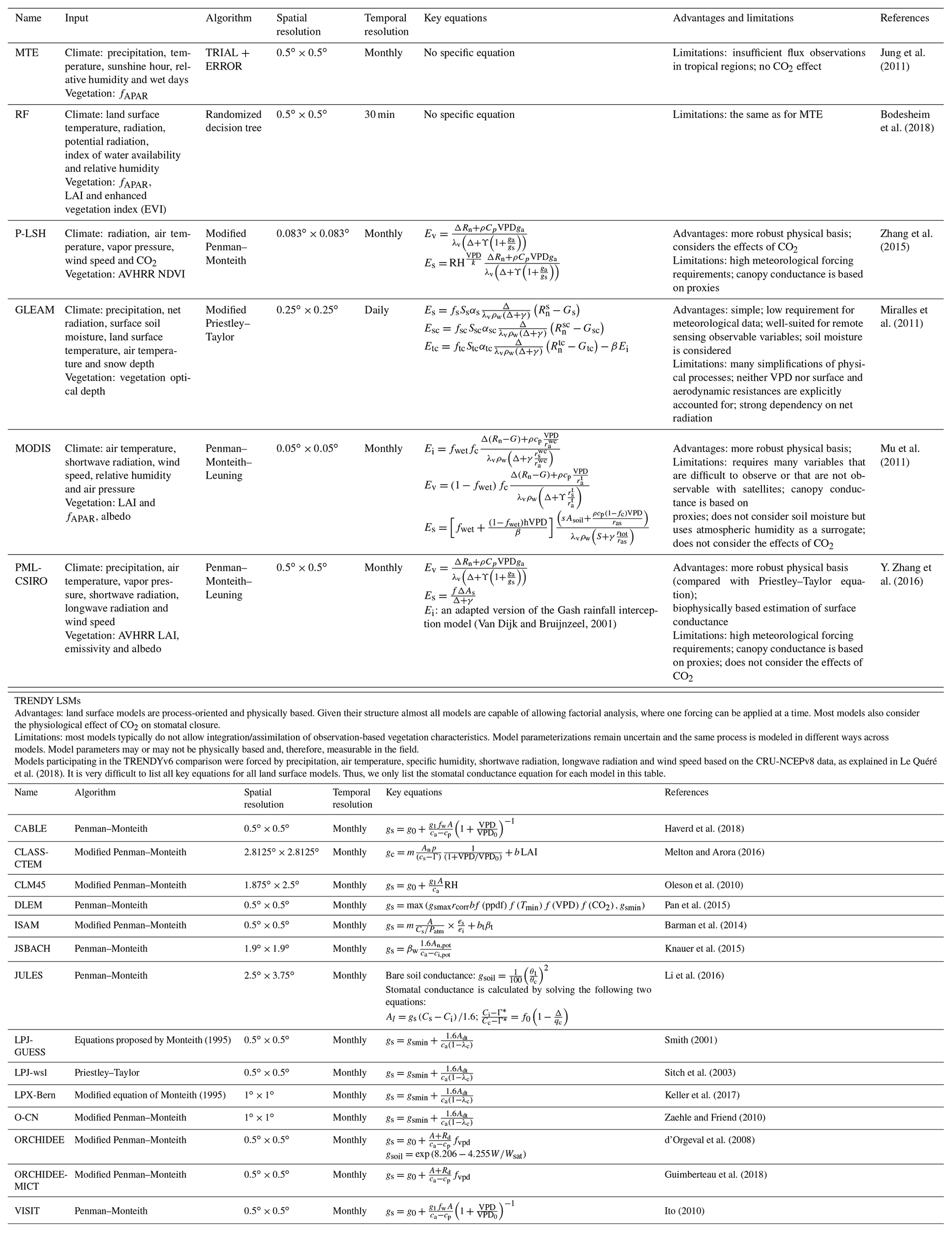
Notes: A: net assimilation rate; A_dt: total daytime net photosynthesis; A_n,pot: unstressed net assimilation rate; b: soil moisture factor; b_t: stomatal conductance intercept; c_a: atmospheric CO₂ concentration; c_c: critical CO₂ concentration;
c_i: internal leaf concentration of CO₂; c_i,pot: internal leaf concentration of CO₂ for unstressed conditions; c_s: leaf surface CO₂ concentration; c_p: CO₂ compensation point; e_s: vapor pressure at leaf surface; e_i: saturation vapor pressure
inside the leaf; E_s: soil evaporation; E_c: canopy evapotranspiration; E_dry: dry canopy evapotranspiration; E_wet: wet canopy evapotranspiration; E_v: canopy transpiration; E_i: canopy interception; E_tc: transpiration from tall canopy;
E_sc: transpiration from short canopy; f: fraction of P to equilibrium soil evaporation; f_s: soil fraction; f_sc: short canopy fraction; f_tc: tall canopy fraction; f_vpd: factor of the effect of leaf-to-air vapor pressure difference; f_w: a function
describing the soil water stress on stomatal conductance; f_wet: relative surface wetness parameter; f₀: the maximum ratio of internal to external CO₂; f(ppdf):limiting factor of photosynthetic photo flux density; f(T_min): limiting factor
of daily minimum temperature; f(VPD): limiting factor of vapor pressure deficit; f(CO₂): limiting factor of carbon dioxide; G: ground energy flux; g_a: aerodynamic conductance; g_m: empirical parameter; g_s: stomatal conductance;
g_smax: maximum stomatal conductance; g_smin: minimum stomatal conductance; g_soil: bare soil conductance; g₀: residual stomatal conductance when the net assimilation rate is 0 ; g₁: sensitivity of stomatal conductance to assimilation,
ambient CO₂ concentration and environmental controls; I: tall canopy interception loss; m: stomatal conductance slope; P_atm: atmospheric pressure; PE_s: potential soil evaporation; PE_canopy: potential canopy evaporation; q_a: specific air
humidity; q_c: critical humidity deficit; q_s: specific humidity of saturated air; r_a: aerodynamic resistance; r_s: stomatal resistance; R_n: net radiation; Rd: day respiration; RH: relative humidity; T_s: actual surface temperature; VPD: vapor
pressure deficit; VPD₀: the sensitivity of stomatal conductance to VPD; W: top soil moisture; W_canopy: canopy water; W_sat: soil porosity; α: Priestley–Taylor coefficient; α_m: empirical parameter; β: a constant accounting for the times
when vegetation is wet; β_t: soil water availability factor between 0 and 1; β_w: a scaling factor to account for water stress; β_s: moisture availability function; ρ: air density; γ: psychrometric constant; λ_v: latent heat of vaporization;
λ_c: ratio of intercellular to ambient partial pressure of CO₂; r_corr: correction factor of temperature and air pressure on conductance; Γ^∗: CO₂ compensation point when leaf day respiration is zero; θ₁: parameter of moisture concentration
in the top soil layer; θ_c: parameter of moisture concentration in the spatially varying critical soil moisture; Δ: slope of the vapor pressure curve.

Four physically based remote sensing datasets, including the Process-based Land Surface Evapotranspiration/Heat Fluxes algorithm (P-LSH), the Global Land Evaporation Amsterdam Model (GLEAM), the Moderate Resolution Imaging Spectroradiometer (MODIS) and the PML-CSIRO (Penman–Monteith–Leuning), and two machine-learning datasets, which are based on random forest (RF) and model tree ensemble (MTE), are used in our study. Both machine-learning and physically based remote sensing datasets (six datasets in total) were considered as benchmark products. The ensemble mean of the benchmark products was calculated as the mean value of all machine-learning and physically based satellite estimates as we treated each benchmark dataset equally.

Three of the four remote-sensing-based physical models quantify ET using PM approaches. P-LSH adopts a modified PM approach coupled with biome-specific canopy conductance determined from NDVI (Zhang et al., 2010). The modified P-LSH model used in this study also accounts for the influences of atmospheric CO₂ concentrations and wind speed on canopy stomatal conductance and aerodynamic conductance (Zhang et al., 2015). The MODIS ET model is based on the algorithm proposed by Cleugh et al. (2007). Mu et al. (2007) improved the model performance through the inclusion of environmental stress into the canopy conductance calculation and by explicitly accounting for soil evaporation by combining the complementary relationship hypothesis with the PM equation. The MODIS ET product (MOD16A3) used in this study was further improved by considering nighttime ET, simplifying the vegetation cover fraction calculation, adding the soil heat flux item, dividing the saturated wet and moist soil, separating the dry and wet canopy, as well as modifying algorithms of aerodynamic resistance, stomatal conductance and boundary layer resistance (Mu et al., 2011). PML-CSIRO adopts the Penman–Monteith–Leuning algorithm, which calculates surface conductance and canopy conductance using a biophysical model instead of classic empirical models. The maximum stomatal conductance is estimated using the trial-and-error method (Y. Zhang et al., 2016). Furthermore, for each grid covered by natural vegetation, the PML-CSIRO model constrains ET at the annual scale using the Budyko hydrometeorological model proposed by Fu (1981). The GLEAM ET calculation is based on the PT equation, which requires fewer model inputs than the PM equation, and the majority of these inputs can be directly achieved from satellite observations. Its rationale is to make the most of information about evaporation contained in the satellite-based environmental and climatic observations (Martens et al., 2017; Miralles et al., 2011). Key variables including air temperature, land surface temperature, precipitation, soil moisture, vegetation optical depth and snow water equivalent are satellite-observed values. Moreover, the extensive usage of microwave remote sensing products in GLEAM ensures the accurate estimation of ET under diverse weather conditions. Here, we use GLEAM v3.2, which has overall better quality than previous versions (Martens et al., 2017).

The first used machine-learning model, MTE, is based on the Tree Induction Algorithm (TRIAL) and Evolving Trees with Random Growth (ERROR) algorithm (Jung et al., 2009). The TRIAL grows model trees from the root node and splits at each node with the criterion of minimizing the sum of squared errors of multiple regressions in both subdomains. ERROR is used to select the model trees that are independent of one another and have the best performance based on the Schwarz criterion. The canopy fraction of absorbed photosynthetic active radiation (f_APAR), temperature, precipitation, relative humidity, sunshine hours and potential radiation are used as explanatory variables to train MTE (Jung et al., 2011). The second machine-learning model is the random forest (RF) algorithm, whose rationale is generating a set of independent regression trees by randomly selecting training samples automatically (Breiman, 2001). Each regression tree is constructed using samples selected by a bootstrap sampling method. After fixing the individual tree in entity, the final result is determined by simple averaging. One merit of the RF algorithm is its capability to handle complicated nonlinear problems and high dimensional data (Xu et al., 2018). For the RF product used in this study, multiple explanatory variables including the enhanced vegetation index, f_APAR, the leaf area index, daytime and nighttime land surface temperature, incoming radiation, top-of-atmosphere potential radiation, the index of water availability and relative humidity were used to train regression trees (Bodesheim et al., 2018).

The 14 LSM-derived ET products were from the Trends and Drivers of the Regional Scale Sources and Sinks of Carbon Dioxide (TRENDY) project (including CABLE, CLASS-CTEM, CLM45, DLEM, ISAM, JSBACH, JULES, LPJ-GUESS, LPJ-wsl, LPX-Bern, O-CN, ORCHIDEE, ORCHIDEE-MICT and VISIT). Daily gridded meteorological reanalyzes from the CRU-NCEPv8 dataset (temperature, precipitation, long- and shortwave incoming radiation, wind speed, humidity and air pressure) were used to drive the LSMs. The TRENDY simulations were performed in year 2017 and contributed to the global carbon budget reported in Le Quéré et al. (2018). We used the results from the S3 simulation from TRENDYv6 (with changing CO₂, climate and land use) over the period from 1982 to 2011, which is a time period consistent with other products derived from remote-sensing-based physical models and machine-learning algorithms.

2.3 Description of other datasets

To quantify the contributions of vegetation greening to terrestrial ET variations, we used the LAI from the TRENDYv6 S3 simulation. We also used the newest version of the Global Inventory Modeling and Mapping Studies LAI data (GIMMS LAI3gV1) as the satellite-derived LAI. GIMMS LAI3gV1 was generated from AVHRR GIMMS NDVI3g using a model derived from an artificial neural network (ANN; Zhu et al., 2013). It covers the period from 1982 to 2016 with bimonthly frequency and has a 1∕12^∘ spatial resolution. To achieve a uniform resolution, all data were resampled to 1∕2^∘ using the nearest neighbor method. Following N. Pan et al. (2018), grids with an annual mean NDVI of less than 0.1 were assumed to be non-vegetated regions and were, therefore, masked out. NDVI data are from the GIMMS NDVI3gV1 dataset. Temperature, precipitation and radiation are from the CRU-NCEPv8 dataset.

2.4 Statistical analysis

The significance of ET trends was analyzed using the Mann-Kendall (MK) test (Kendall, 1955; Mann, 1945). It is a rank-based nonparametric method that has been widely applied for detecting trends in hydro-climatic time series (Sayemuzzaman and Jha, 2014; Yue et al., 2002). The Theil–Sen estimator was applied to estimate the magnitude of the slope. The advantage of this method over an ordinary least squares estimator is that it limits the influence of the outliers on the slope (Sen, 1968).

Terrestrial ET interannual variability (IAV) is mainly controlled by variations in temperature, precipitation and shortwave solar radiation (Zeng et al., 2018b; Zhang et al., 2015). In this study, we performed partial correlation analyses between ET and these three climatic variables at an annual scale for each grid cell to explore climatic controls on ET IAV. Variability caused by climatic variables was assessed through the square of partial correlation coefficients between ET and temperature, precipitation and radiation. We chose partial correlation analysis because it can quantify the linkage between ET and a single environmental driving factor while controlling the effects of the other remaining environmental factors. Partial correlation analysis is a widely applied statistical tool to isolate the relationship between two variables from the confounding effects of many correlated variables (Anav et al., 2015; Jung et al., 2017; Peng et al., 2013). All variables were first detrended in the statistical correlation analysis, as we focus on the interannual relationship. The study period is from 1982 to 2011 for all models except MODIS and random forest, which have a temporal coverage that is limited to 2001–2011 because of data availability.

To quantify the contribution of vegetation greening to terrestrial ET, we separated the trend in terrestrial ET into four components induced by climatic variables and vegetation dynamics by establishing a multiple linear regression model between global ET and temperature, precipitation, shortwave radiation and LAI (Eqs. 3, 4):

$$\begin{array}{}\text{(3)}& {\displaystyle }\begin{array}{rl}\mathit{\delta }\left(\mathrm{ET}\right)& ={\displaystyle \frac{\partial \left(\mathrm{ET}\right)}{\partial \left(\mathrm{LAI}\right)}}\mathit{\delta }\left(\mathrm{LAI}\right)+{\displaystyle \frac{\partial \left(\mathrm{ET}\right)}{\partial T}}\mathit{\delta }\left(\mathrm{T}\right)+{\displaystyle \frac{\partial \left(\mathrm{ET}\right)}{\partial \left(P\right)}}\mathit{\delta }\left(P\right)\\ & +{\displaystyle \frac{\partial \left(\mathrm{ET}\right)}{\partial R}}\mathit{\delta }\left(R\right)+\mathit{\epsilon }\end{array}\text{(4)}& {\displaystyle }\mathit{\delta }\left(\mathrm{ET}\right)={\mathit{\gamma }}_{\mathrm{ET}}^{\mathrm{LAI}}\mathit{\delta }\mathrm{LAI}+{\mathit{\gamma }}_{\mathrm{ET}}^T\mathit{\delta }T+{\mathit{\gamma }}_{\mathrm{ET}}^P\mathit{\delta }P++{\mathit{\gamma }}_{\mathrm{ET}}^R\mathit{\delta }R+\mathit{\epsilon },\end{array}$$

where ${\mathit{\gamma }}_{\mathrm{ET}}^{\mathrm{LAI}}$, ${\mathit{\gamma }}_{\mathrm{ET}}^T$, ${\mathit{\gamma }}_{\mathrm{ET}}^P$ and ${\mathit{\gamma }}_{\mathrm{ET}}^R$ are the sensitivities of ET to the leaf area index (LAI), air temperature (T), precipitation (P) and radiation (R), respectively. ε is the residual, representing the impacts of other factors.

After calculating ${\mathit{\gamma }}_{\mathrm{ET}}^{\mathrm{LAI}}$, ${\mathit{\gamma }}_{\mathrm{ET}}^T$, ${\mathit{\gamma }}_{\mathrm{ET}}^P$ and ${\mathit{\gamma }}_{\mathrm{ET}}^R$, the contribution of the trend in factor i (Trend(i)) to the trend in ET (Trend(ET)) can be quantified as follows:

$$\begin{array}{}\text{(5)}& \mathrm{Contri}\left(i\right)=\left({\mathit{\gamma }}_{\mathrm{ET}}^i\times \mathrm{Trend}\left(i\right)\right)/\mathrm{Trend}\left(\mathrm{ET}\right).\end{array}$$

In performing multiple linear regression, we used the GIMMS LAI for both remote-sensing-based physical models and machine-learning methods as well as the individual TRENDYv6 LAI for each TRENDY model. The gridded data of temperature, precipitation and radiation are from CRU-NCEPv8.

3 Results

3.1 The ET magnitude estimated by multiple models

The multiyear ensemble mean of annual global terrestrial ET from 2001 to 2011 derived by machine-learning methods, remote-sensing-based physical models and the TRENDY models agreed well, with values ranging from 589.6 to 617.1 mm yr⁻¹. However, substantial differences existed among individual models (Fig. 1). LPJ-wsl (455.3 mm yr⁻¹) and LPX-Bern (453.7 mm yr⁻¹) estimated significantly lower ET than other models, even in comparison with most previous studies focusing on earlier periods (Table S1 in the Supplement). On the contrary, JULES gave the largest ET estimate (697.3 mm yr⁻¹, which is equal to 7.57×10⁴ km³ yr⁻¹) among all models, and showed an obvious increase in ET compared with its estimation from 1950 to 2000 (6.5×10⁴ km³ yr⁻¹, Table S1).

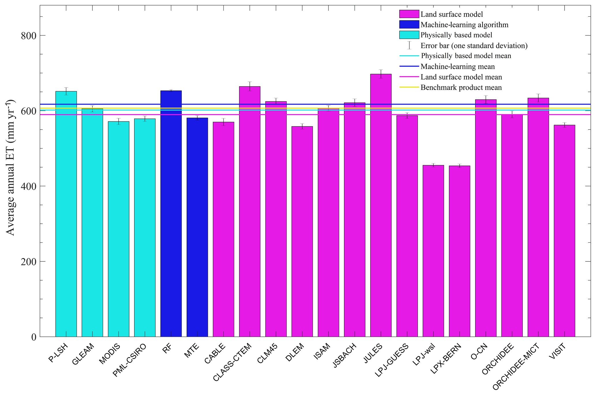
Figure 1 Average annual global terrestrial ET estimated by each model during the period from 2001 to 2011. Error bars represent the standard deviation of each model. The four lines indicate the mean value of each category.

3.2 Spatial patterns of global terrestrial ET

As shown in Fig. 2, the spatial patterns of the multiyear average annual ET of different categories were similar. ET was highest in the tropics and low in the northern high latitudes and arid regions such as Australia, central Asia, the western US and the Sahel. Compared with remote-sensing-based physical models and LSMs, machine-learning methods obtained a smaller spatial gradient. In general, latitudinal profiles of ET estimated using different approaches were also consistent (Fig. 3). However, machine-learning methods gave higher ET estimate at high latitudes and lower ET in the tropics compared with other approaches. In the tropics, LSMs have significantly larger uncertainties than benchmark products, and the standard deviation of LSMs is about 2 times higher than that of benchmark products (Fig. 3). At other latitudes, LSMs and benchmark ET products generally have comparable uncertainties. The largest difference in ET in the different categories was found in the Amazon Basin (Fig. 2). In most regions of the Amazon Basin, the mean ET of remote sensing physical models is more than 200 mm yr⁻¹ higher than the mean ET of LSMs and machine-learning methods. For individual ET estimates, the largest uncertainty was also found in the Amazon Basin. MODIS, VISIT and CLASS-CTEM estimated that the annual ET was higher than 1300 mm in the majority of Amazon, whereas JSBACH and LPJ-wsl estimated an ET value lower than 800 mm yr⁻¹ (Fig. S1). As is shown in Fig. S2, the differences in ET estimates among TRENDY models were larger than those among benchmark estimates for tropical and humid regions. The uncertainty of ET estimates from LSMs is particularly large in the Amazon Basin, where the standard deviation of LSM estimates is more than 2 times larger than that of benchmark estimates. It is noteworthy that, in arid and semiarid regions such as western Australia, central Asia, northern China and the western US, the difference in ET estimates among LSMs is significantly smaller than those among remote sensing models and machine-learning algorithms.

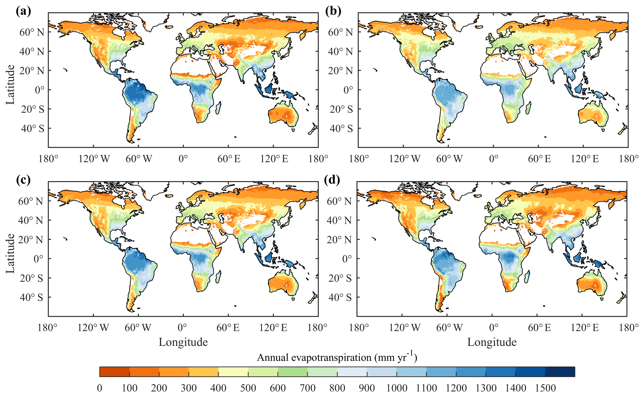
Figure 2 Spatial distributions of the mean annual ET derived from (a) remote-sensing-based physical models, (b) machine-learning algorithms, (c) benchmark datasets and (d) the TRENDY LSMs' ensemble mean, respectively.

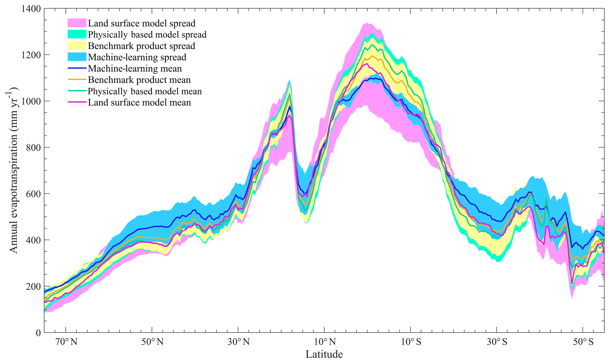
Figure 3 Latitudinal profiles of the mean annual ET for different categories of models. Each line represents the mean value of the corresponding category, and the shading represents the interval of 1 standard deviation.

3.3 Interannual variations in global terrestrial ET

The ensemble mean interannual variability (IAV) of remote sensing ET estimates and LSM ET estimates showed similar spatial patterns (Fig. 4). Both remote sensing physical models and LSMs presented low IAV in ET in the northern high latitudes but high IAV in ET in the southwestern US, India, sub-Saharan Africa, the Amazon and Australia. In contrast, the IAV of machine-learning-based ET was much weaker. In most regions, the IAV of machine-learning ET is lower than 40 % of the IAV of remote sensing physical ET and LSM ET, and this phenomenon is especially pronounced in tropical regions. Further investigation into the spatial patterns of ET IAV for individual models showed that the two machine-learning methods performed equally with respect to estimating spatial patterns of ET IAV (Fig. S4). In contrast, differences in ET IAV among remote sensing physical estimates and LSM estimates were much larger. LSMs showed the largest differences in the IAV of ET in tropical regions. For example, CABLE and JULES obtained an ET IAV of less than 15 mm yr⁻¹ in most regions of the Amazon Basin, whereas LPJ-GUESS predicted an ET IAV of more than 60 mm yr⁻¹. Figure 5 shows that remote sensing physical ET and LSM ET had comparable IAV north of 20^∘ S, but the IAV of the machine-learning-based ET was much lower in this region. In the region south of 20^∘ S, TRENDY ET showed the largest IAV, followed by those of remote sensing physical ET and machine-learning estimates. The three approaches agreed on that ET IAV in the Southern Hemisphere was generally larger than that in the Northern Hemisphere.

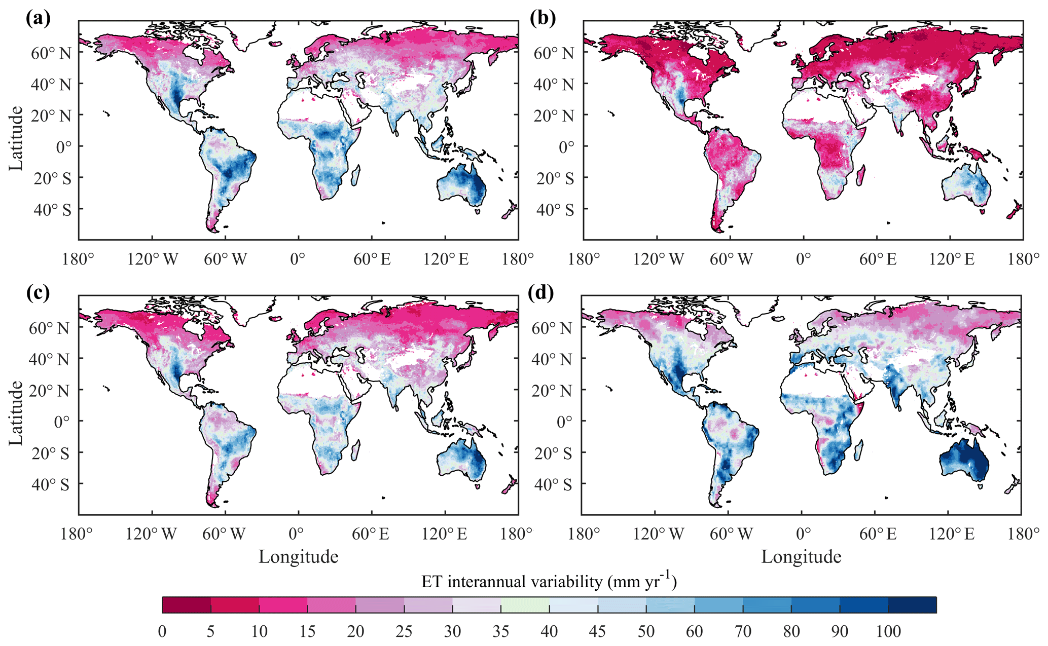
Figure 4 Spatial distributions of the interannual variability in ET derived from (a) remote-sensing-based physical models, (b) machine-learning algorithms, (c) benchmark datasets and (d) the TRENDY LSMs' ensemble mean, respectively. The study period used in this study for the interannual variability analysis is from 1982 to 2011.

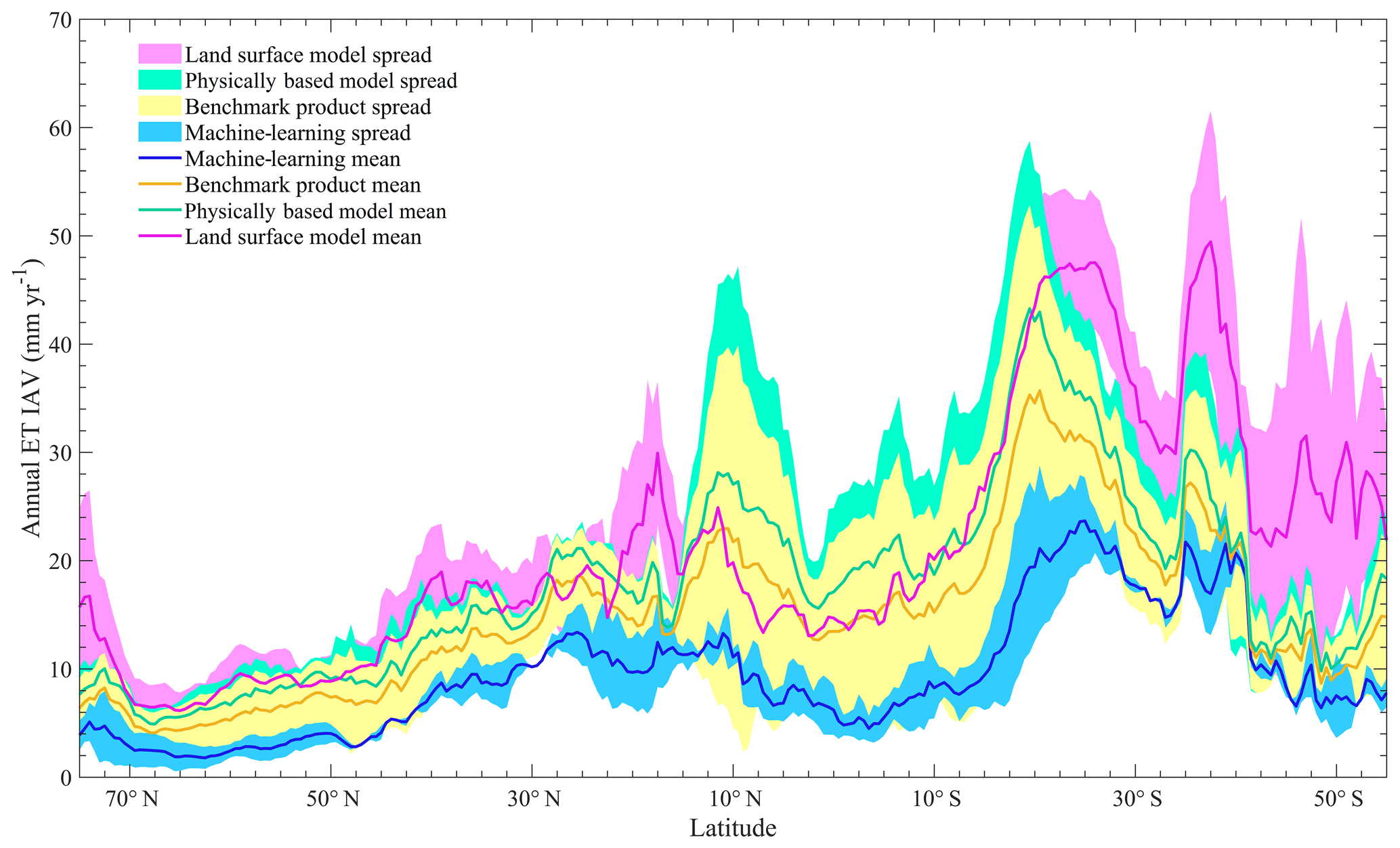
Figure 5 Latitudinal profiles of ET IAV for different categories of models. Each line represents the mean value of the corresponding category, and the shading represents the interval of 1 standard deviation.

3.4 Climatic controls on ET

According to the ensemble remote sensing models, temperature and radiation dominated ET IAV in northern Eurasia, northern and eastern North America, southern China, the Congo River basin, and the southern Amazon River basin, while precipitation dominated ET IAV in arid regions and semiarid regions (Fig. 6a). The ensemble machine-learning algorithms had a similar pattern, but they suggested a stronger control of radiation in the Amazon Basin and a weaker control of precipitation in several arid regions such as central Asia and northern Australia (Fig. 6b). In comparison, the ensemble LSMs suggested the strongest control of precipitation on ET IAV (Fig. 6). According to the ensemble LSMs, ET IAV was dominated by precipitation IAV in most regions of the Southern Hemisphere and at northern low latitudes. Temperature and radiation only controlled northern Eurasia, eastern Canada and part of the Amazon Basin (Fig. 6d). As is shown in Fig. S6, the majority of LSMs agreed on the dominant role of precipitation in controlling ET in regions south of 40^∘ N. However, the pattern of climatic controls in the ORCHIDEE-MICT model is quite unique and different from all of the other LSMs. According to the ORCHIDEE-MICT model, radiation and temperature dominate ET IAV in more regions, and precipitation only controls ET IAV in eastern Brazil, northern Russia, central Europe and a part of tropical Africa. As ORCHIDEE-MICT was developed from ORCHIDEE, the dynamic root parameterization in ORCHIDEE-MICT may explain why ET is less driven by precipitation compared with ORCHIDEE (Haverd et al., 2018). It is noted that two machine-learning algorithms, MTE and RF, showed significant discrepancies in the spatial pattern of dominant climatic factors. According to the result from MTE, temperature controlled ET IAV in regions north of 45^∘ N, the eastern US, southern China and the Amazon Basin (Fig. S6e). By contrast, RF suggested that precipitation and radiation dominated ET IAV in these regions (Fig. S6f).

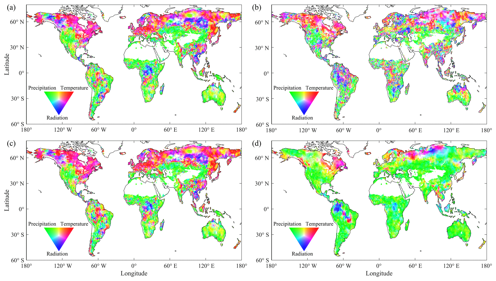
Figure 6 Spatial distributions of climatic controls on the interannual variation of ET derived from the ensemble means of remote-sensing-based physical models (a), machine-learning algorithms (b), benchmark data (c) and the TRENDY LSMs (d). (Red denotes temperature, green denotes precipitation and blue denotes radiation.)

3.5 Long-term trends in global terrestrial ET

All approaches suggested an overall increasing trend in global ET during the period from 1982 to 2011 (Fig. 7), although ET decreased from 1998 to 2009. This result is consistent with previous studies (Jung et al., 2010; Lian et al., 2018; Zhang et al., 2015). Remote sensing physical models indicated the largest increase in ET (0.62 mm yr⁻²), followed by the machine-learning method (0.38 mm yr⁻²) and land surface models (0.23 mm yr⁻²). The mean ET of all categories except LSMs significantly increased during the study period (p<0.05). It is noted that the ensemble mean ET values of different categories are statistically correlated with each other (p<0.001), even if the driving forces of different ET approaches are different.

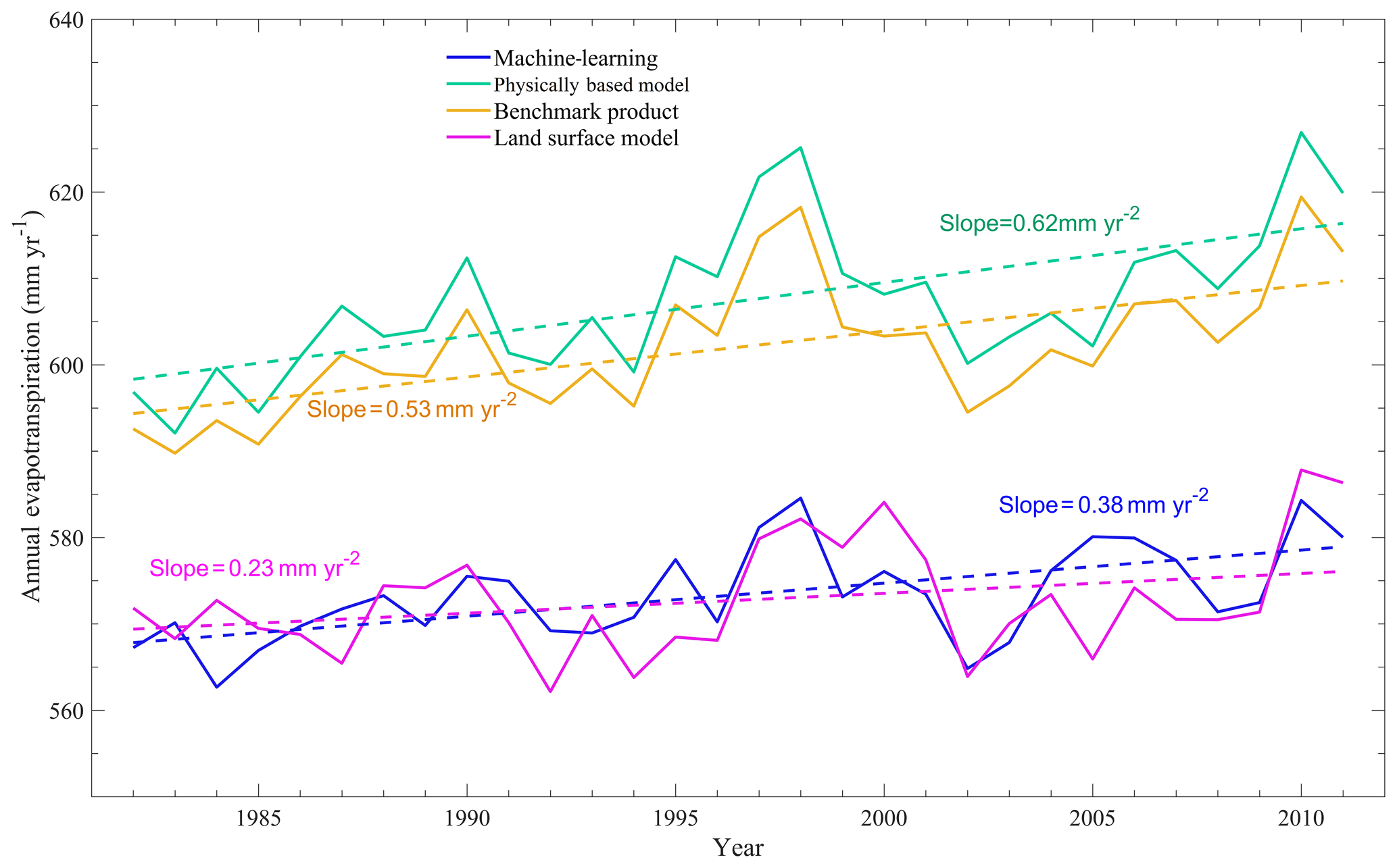
Figure 7 Interannual variations in global terrestrial ET estimated using different categories of approaches.

Table 2 Interannual variability (IAV – denoted as standard deviation) and the trend of global terrestrial ET from 1982 to 2011 and the contribution of vegetation greening to the ET trend. (RS refers to remote sensing.)

^∗ Suggests significance at the 95 % confidence level (p<0.05).

All remote sensing and machine-learning estimates indicate a significant increasing trend in ET during the study period (p<0.05), although the increase rate of P-LSH (1.07 mm yr⁻²) is more than 3 times as large as that of GLEAM (0.33 mm yr⁻²). Nevertheless, there is a larger discrepancy among LSMs in terms of the ET trend. The majority of LSMs (10 of 14) suggest an increasing trend with an average trend of 0.34 mm yr⁻² (p<0.05), and eight of them are statistically significant (see Table 2). However, four LSMs (JSBACH, JULES, ORCHIDEE and ORCHIDEE-MICT) suggest a decreasing trend with an average trend of −0.12 mm yr⁻² (p>0.05). Among the four decreasing trends, only the trend of ORCHIDEE-MICT (−0.34 mm yr⁻²) is statistically significant (p<0.05).

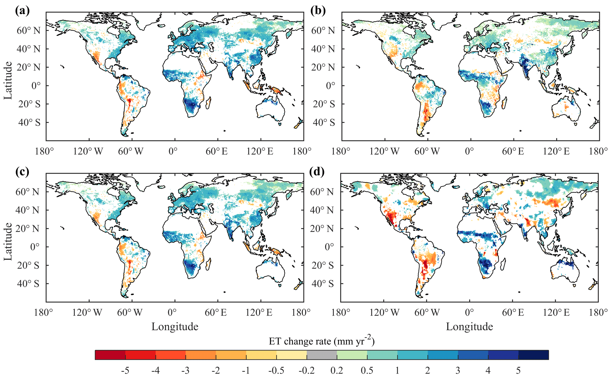
Figure 8 Spatial distributions of ET trends from 1982 to 2011 derived from (a) remote-sensing-based physical models, (b) machine-learning algorithms, (c) benchmark datasets and (d) the TRENDY LSMs' ensemble mean, respectively. Regions with nonsignificant trends were excluded.

According to Fig. 8, the ensemble means of all the three approaches showed increasing trends in ET over western and southern Africa, western India and northern Australia, and decreasing ET over the western US, southern South America and Mongolia. Discrepancies in ET trends mainly appeared in eastern Europe, eastern India and central China. LSMs also suggested a larger area of decreasing ET in both North America and South America. Although the differences in ET trends among individual models were larger than those among the ensemble means of different approaches, the majority of models agreed that ET increased in western and southern Africa, and decreased in the western US and southern South America (Fig. S2). For both remote sensing estimates and LSM estimates, ET trends in the Amazon Basin had large uncertainty: P-LSH, CLM45 and VISIT suggested a large area of increasing ET, whereas GLEAM, JSBACH and ORCHIDEE suggested a large area of decreasing ET.

3.6 Impacts of vegetation changes on ET variations

During the period from 1982 to 2011, global LAI trends estimated from remote sensing data and from the ensemble LSMs are $\mathrm{2.51}\times {\mathrm{10}}^{-\mathrm{3}}$ m² m⁻² yr⁻¹ (p<0.01) and $\mathrm{4.63}\times {\mathrm{10}}^{-\mathrm{3}}$ m² m⁻² yr⁻¹ (p<0.01), respectively (Table 2). All LSMs suggested a significant increasing trend in global LAI (greening). For both benchmark estimates and LSM estimates, it was found that the spatial pattern of trends in ET matched well with that of trends in the LAI (Figs. 8c, d, S5a, b), indicating significant effects of vegetation dynamics on ET variations. According to the results of the multiple linear regression, all models agreed that greening of the Earth since the early 1980s intensified terrestrial ET (Table 2), although there was a significant discrepancy in the magnitude of ET intensification which varied from 0.04 to 0.70 mm yr⁻². The ensemble LSMs suggested a smaller ET increase (0.23 mm yr⁻2) than the ensemble remote sensing physical models (0.62 mm yr⁻²) and machine-learning algorithm (0.38 mm yr⁻²). Nevertheless, the greening-induced ET intensification estimated by LSMs (0.37 mm yr⁻²) is larger than that estimated by remote sensing models (0.28 mm yr⁻²) and machine-learning algorithms (0.09 mm yr⁻²), as LSMs suggested a stronger greening trend than remote sensing models. The contribution of vegetation greening to ET intensification estimated by the ensemble LSMs is larger than 100 %, whereas the contributions estimated by the ensemble remote sensing physical models (0.62 mm yr⁻²) and machine-learning algorithm are smaller than 50 %. Although TRENDY LSMs were driven by the same climate data and remote sensing physical models were driven by varied climate data, TRENDY LSMs still showed a larger discrepancy in terms of the effect of vegetation greening on terrestrial ET than remote sensing physical models due to the significant differences in both LAI trends (1.74–$\mathrm{13.63}\times {\mathrm{10}}^{-\mathrm{3}}$ m² m⁻² yr⁻¹) and the sensitivities of ET to the LAI (4.04–217.39 mm yr⁻² m⁻² m⁻²). In comparison, remote sensing physical models had smaller discrepancies in terms of the sensitivity of ET to LAI (55.78–143.43 mm yr⁻² m⁻² m⁻²).

4 Discussion and perspectives

4.1 Sources of uncertainty

4.1.1 Uncertainty in the ET estimation of the Amazon Basin

LSMs show large discrepancies in the magnitude and trend of ET in the Amazon Basin (Figs. 3, S3). However, it is challenging to identify the uncertainty sources. Given that the TRENDY LSMs used uniform meteorological inputs, the discrepancies in ET estimates among the participating models mainly arise from the differences in the underlying model structures and parameters. One potential source of uncertainty is the parameterization of root water uptake. In the Amazon Basin, a deep root depth has been confirmed using field measurements (Nepstad et al., 2004). However, many LSMs have an unrealistically shallow rooting depth (generally less than 2 m), thereby neglecting the existence and significance of deep roots. The incorrect root distributions enlarge the differences in plant available water and root water uptake, producing large uncertainties in ET. In addition, differences in the parameterization of other key processes pertinent to ET such as LAI dynamics (Fig. S5), canopy conductance variations (Table 1), water movements in the soil (Abramopoulos et al., 1988; Clark et al., 2015; Noilhan and Mahfouf, 1996) and soil moisture's control on transpiration (Purdy et al., 2018; Szutu and Papuga, 2019) also increase the uncertainty in ET. The abovementioned processes are not independent of each other but interact in complex ways to produce the end result.

4.1.2 Uncertainty in the ET estimation of arid and semiarid regions

In arid and semiarid regions, benchmark products show much larger differences in the magnitude of ET than LSMs (Fig. S2). One cause of this phenomenon is the difference in meteorological forcing. Remote sensing and machine-learning datasets used different forcing data. For precipitation, RF used the CRUNCEPv6 dataset, MTE used the Global Precipitation Climatology Centre (GPCC) dataset, MODIS used the Global Modeling and Assimilation Office (GMAO) dataset, GLEAM used the Multi-Source Weighted-Ensemble Precipitation (MSWEP) dataset, PML-CSIRO used the Princeton Global Meteorological Forcing (PGF) and the WATCH Forcing Data ERA-Interim (WFDEI) datasets, and P-LSH used data derived from four independent sources. As precipitation is the key climatic factor controlling ET in arid and semiarid regions (Fig. 6), discrepancies between different forcing precipitation (Sun et al., 2018) may be the main source of large uncertainty there. In comparison, the uniform forcing data reduced the inter-model range in ET estimates from the TRENDY LSMs. Nevertheless, it is noted that the congruence across LSM ET estimates does not necessarily mean that they are the correct representation of ET. The narrower inter-model range may suggest shared biases. All remote sensing models and machine-learning algorithms except GLEAM do not explicitly take the effects of soil moisture into account (Table S1). Given that soil moisture is pivotal to both canopy conductance and soil evaporation in arid and semiarid regions (A et al., 2019; De Kauwe et al., 2015; Medlyn et al., 2015; Purdy et al., 2018), the lack of soil moisture information also increases the bias in ET estimation. In addition, the accuracy of remote sensing data itself is also an uncertainty source. The retrieval of key land surface variables, such as the leaf area index and surface temperature, is influenced by vegetation architecture, solar zenith angle and satellite observational angle, particularly over heterogeneous surface (Norman and Becker, 1995).

4.1.3 Uncertainty in the ET IAV in the Southern Hemisphere

In regions south of 20^∘ S (including Australia, southern Africa and southern South America), the ET IAV of remote sensing models and machine-learning algorithms is lower than that of LSMs (Figs. 4, 5), although their spatial patterns are similar. In these regions, GLEAM, the only remote sensing model that explicitly considers the effects of soil moisture, has larger ET IAV than other remote sensing models and has similar ET IAV to LSMs (Fig. S4). This could imply that most of the existing remote sensing models may underestimate ET IAV in the Southern Hemisphere because the effects of soil moisture are not explicitly considered. Machine-learning algorithms show much lower IAV than other models (Figs. 4, S4). The main reason for this is that ET IAV is partly neglected in the training process, as the magnitude of ET IAV is usually smaller than the spatial and seasonal variability (Anav et al., 2015; Jung et al., 2019). Moreover, the IAV of satellite-based key land surface variables such as the LAI, f_APAR and surface temperature may be not reliable because of the effects of clouds, which, in turn, affects the estimation of the IAV of satellite-based ET. It is noted that LSM ET IAV shows large differences at latitudes south of 20^∘ S (Fig. 5). This divergence in ET IAV indicates that LSMs require better representation of the ET response to climate in the Southern Hemisphere.

4.1.4 Uncertainty in the global ET trend

All three categories of ET models detected an overall increasing trend in global terrestrial ET since the early 1980s, which is in agreement with previous studies (Mao et al., 2015; Miralles et al., 2014; Zeng et al., 2018a, b, 2014; Zhang et al., 2015; Y. Zhang et al., 2016). Benchmark products generally suggested stronger ET intensification than LSMs. The weaker ET intensification in LSMs may be induced by the response of stomatal conductance to the increasing atmospheric CO₂ concentration. Increasing CO₂ affects ET in two ways: on the one hand, increasing CO₂ can effectively reduce stomatal conductance and, thus, decrease transpiration (Heijmans et al., 2001; Leipprand and Gerten, 2006; Swann et al., 2016); on the other hand, it can increase vegetation productivity and, thus, increase LAI. For benchmarks, the second effect could be captured by remotely sensed LAI, NDVI or f_APAR, whereas the first effect was neglected by all models except P-LSH (Zhang et al., 2015). In contrast, both effects were modeled in all TRENDY LSMs.

LAI dynamics have significant influences on ET. The increased LAI trend (greening) since the early 1980s has been reported by previous studies (Mao et al., 2016; Zhu et al., 2016) and has also been confirmed by remote sensing data and all of the TRENDY LSMs used in this study (Table 2, Fig. S5). Zhang et al. (2015) found that the increasing trend of global terrestrial ET from 1982 to 2013 was mainly driven by an increase in the LAI and the enhanced atmosphere water demand. Using a land–atmosphere coupled global climate model (GCM), Zeng et al. (2018b) further estimated that global LAI increased by about 8 %, resulting in an increase of 0.40±0.08 mm yr⁻² in global ET (contributing to 55 %±25 % of the ET increase). This number is close to the estimates of ensemble LSMs (0.37±0.18 mm yr⁻²). In comparison, the remote sensing models and machine-learning algorithms used in this study suggested smaller greening-induced ET increases. It is noted that TRENDY LSMs still showed a larger discrepancy in terms of the effect of vegetation greening on terrestrial ET than remote sensing physical models (Table 2) due to the significant differences in the LAI trend (1.74–$\mathrm{13.63}\times {\mathrm{10}}^{-\mathrm{3}}$ m² m⁻² yr⁻¹) and in the sensitivity of ET to LAI (4.04–217.39 mm yr⁻² m⁻² m⁻²). Uncertainties in the LAI trend may arise from inappropriate carbon allocations and deficiencies in responding to water deficits (Anav et al., 2013; Hu et al., 2018; Murray-Tortarolo et al., 2013; Restrepo-Coupe et al., 2017). Additionally, for machine-learning algorithms, the results from insufficient long-term in situ measurements and sparse observations in tropical, boreal and arid regions imply that there are likely deficiencies in representing the temporal variations.

4.1.5 Lack of knowledge of the effects of irrigation

Irrigation accounts for about 90 % of human consumptive water use and largely affects ET in irrigated croplands (Siebert et al., 2010). Global water withdrawals for irrigation were estimated to be within the range of 1161–3800 km³ yr⁻¹ around the year 2000, and they largely increased during the period from 2000 to 2014 (Chen et al., 2019). However, none of the remote-sensing-based physical models and machine-learning algorithms explicitly accounted for the effects of irrigation on ET, although these effects could be taken into account to some extent by using observed LAI, NDVI or f_APAR to drive the models (Zhang et al., 2015). Considering that annual ET may surpass annual precipitation in cropland areas, Y. Zhang et al. (2016) only used the Budyko hydrometeorological model to constrain the PML-CSIRO model in grids covered by non-crop vegetation. However, the process of irrigation affecting evaporation was still not taken into consideration. For TRENDY LSMs, only 2 of 14 models (DLEM and ISAM) included irrigation processes (Le Quéré et al., 2018). Therefore, the effects of irrigation are largely neglected in existing global ET datasets, which reduces the accuracy of local ET estimates in regions with a large proportion of irrigated cropland.

4.1.6 ET variability across the precipitation gradient and its planetary boundary

Precipitation is the source of terrestrial ET. According to Fig. 9a, the vast majority of models agree that ET has the largest IAV in regions with annual precipitation between 700 and 1000 mm, although the magnitude of ET IAV has substantial discrepancies among different models. The low ET IAV in arid and semiarid regions does not mean that ET is stable in these regions. In fact, ET has the largest coefficient of variation (CoV – the ratio of ET standard deviation to ET mean value) in arid regions, and all models show a clear negative trend in the CoV with increasing precipitation (Fig. 9b). This is mainly caused by the large CoV of precipitation in arid regions (Fatichi et al., 2012).

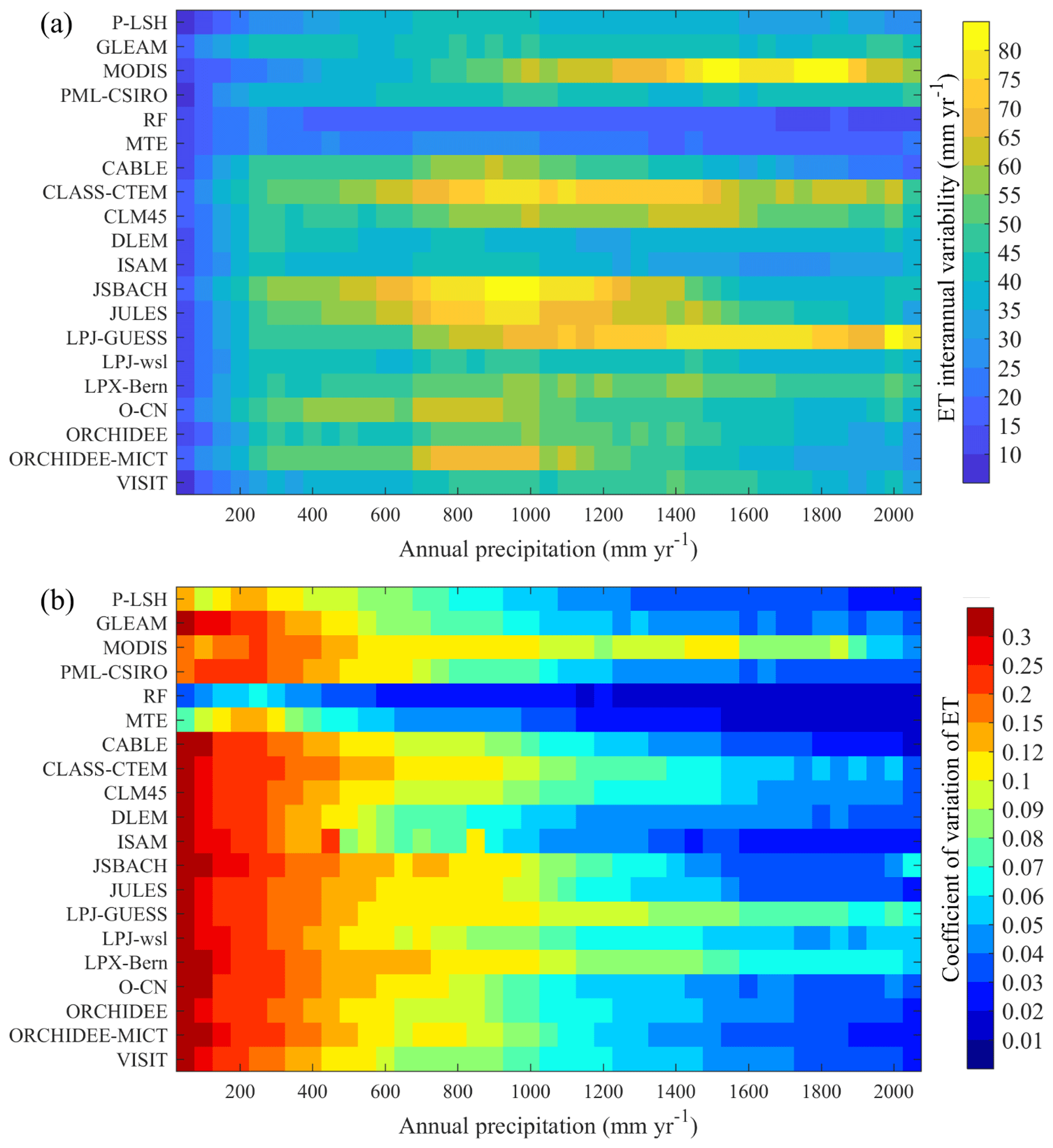
Figure 9 Interannual variability (a) and the coefficient of variation (b) of ET for each 50 mm interval of mean annual precipitation.

In comparison, terrestrial ET shows a much lower IAV at the global scale (Table 2), with values ranging from 4.8 to 12.2 mm yr⁻¹ (1 standard deviation), which only equates to 1.0 %–1.8 % of the global annual mean ET. The model results suggest that global terrestrial ET stabilizes at about 6.74×10⁴ km³ yr⁻¹ (603 mm yr⁻¹), which is close to previous estimates (Alton et al., 2009; Mueller et al., 2011; Oki and Kanae, 2006; Zeng et al., 2012). The stability of global terrestrial ET is probably based on partitioning the solar constant and suggests that droughts in one place are balanced by excess rain in other places; thus, it all evens out at a global scale. This implies that ET also has a potential planetary boundary, a suggestion made by Running (2012) on net primary production (NPP) as a planetary boundary. ET integrates four aspects of the current planetary boundaries defined by Steffen et al. (2015): climate change, freshwater use, land-system change and biochemical flows. Given the importance of ET with respect to linking terrestrial water, carbon, nutrient and energy cycles, more studies on the ET planetary boundary are needed in the context of intensifying global change and increasing anthropogenic perturbations to the Earth system.

In short, the multi-model intercomparison indicates that considerable uncertainty exists in both the temporal and spatial variations in global ET estimates, although a large portion of models adopt similar ET algorithms (Table 1). The major uncertainty source is different for different types of models and regions. The uncertainty is induced by multiple factors, including problems pertinent to parameterization of land processes, lack of in situ measurements, remote sensing acquisition, scaling effects and meteorological forcing. Based on the results of different approaches, we suggest that global terrestrial ET also has a potential planetary boundary, with the value being about 6.74×10⁴ km³ yr⁻¹ (603 mm yr⁻¹), which is consistent with previous estimates.

4.2 Recommendations for future development

4.2.1 Remote-sensing-based physical methods

Over the past few decades, the development of remote sensing technologies has contributed to a boom in various ET estimation methods. However, there is still much room for remote sensing technologies to improve (Fisher et al., 2017). The development of new platforms and sensors that have improved global spatiotemporal coverage and using multiband, multisource remote sensing data are the key points. Planned or newly launched satellites, such as NASA's GRACE Follow-On (GRACE-FO) mission and the ECOsystem Spaceborne Thermal Radiometer Experiment on Space Station (ECOSTRESS) mission, will improve the accuracy of terrestrial ET estimates. ECOSTRESS's thermal infrared (TIR) multispectral scanner is capable of monitoring diurnal temperature patterns at high resolutions, which provides insights into plant response to water stress as well as the means to understand sub-daily ET dynamics (Hulley et al., 2017). GRACE Follow-On observations can be used to constrain subsurface lateral water transfers, which helps to correct soil moisture and subsequently improves the accuracy of ET estimates (Rouholahnejad and Martens, 2018). Moreover, building integrated methods that fuse different ET estimates or the upstream satellite-based biophysical variables from different platforms and the other forcing data will be helpful to improve the accuracy and spatiotemporal coverage of ET (Ke et al., 2016; Ma et al., 2018; Semmens et al., 2016).

The theories and retrieval algorithms of ET and the related key biophysical variables also need to be further improved. For example, the method for calculating canopy conductance may be improved by integrating remote-sensing-based solar-induced chlorophyll fluorescence (SIF) data. SIF data from existing Global Ozone Monitoring Experiment-2 (GOME-2), Orbiting Carbon Observatory-2 (OCO-2) and TROPOspheric Monitoring Instrument (TROPOMI) satellite instruments as well as the forthcoming OCO-3 and Geostationary Carbon Cycle Observatory (GeoCarb) satellites provide a good opportunity to diagnose transpiration and to examine ET partitioning at multiple spatiotemporal scales (Pagán et al., 2019; Stoy et al., 2019; Sun et al., 2017). Theoretical advancements in nonequilibrium thermodynamics and maximum entropy production (MEP) could be incorporated into the classical ET theories (Xu et al., 2019; K. Zhang et al., 2016). In addition, quantifying the effects of CO₂ fertilization on stomatal conductance is pivotal for remote sensing models to capture the long-term trend of terrestrial ET.

Most existing remote-sensing-based ET studies have focused on total ET; however, the partitioning of ET between transpiration, soil evaporation, and canopy interception may show significant divergence even though the total ET is accurately estimated (Talsma et al., 2018b). In current remote-sensing-based ET models, soil evaporation, which is sensitive to precipitation events and soil moisture, is the component with the largest error (Talsma et al., 2018a). Therefore, incorporating the increasingly accessible satellite-based precipitation, soil moisture observations and soil property data will contribute to the improvement of the soil evaporation estimation. Meanwhile, the consideration of soil evaporation under herbaceous vegetation and canopy will also reduce the errors.

4.2.2 Machine-learning methods

It is well known that the capability of machine-learning algorithms to provide accurate ET estimates largely depends on the representativeness of the training datasets with respect to describing ecosystem behaviors (Yao et al., 2017). As a result, machine-learning algorithms may not perform well outside the range of the data used for their training. Unfortunately, long-term field observations in northern temperate regions are still insufficient. This is an important cause of the small spatial gradient and small IAV of machine-learning ET. Given that remote sensing is capable of providing broad coverage of key biophysical variables at reasonable spatial and temporal resolutions, one way to overcome this challenge is to exclusively use remote sensing observations as training data (Jung et al., 2019; Poon and Kinoshita, 2018). Another simple way to make the IAV of machine-learning ET more realistic is to normalize the yearly anomalies when comparing them with ET estimates from LSMs and remote sensing physical models (Jung et al., 2019). New machine-learning techniques, including the extreme learning machine and the adaptive neuro-fuzzy inference system, can be used to improve the accuracy of ET estimation (Gocic et al., 2016; Kişi and Tombul, 2013). Emerging deep-learning methods such as recurrent neural network (RNN) and long short-term memory (LSTM) have the potential to outcompete conventional machine-learning methods in modeling ET time series (Reichstein et al., 2018, 2019). Almost all machine-learning datasets used precipitation rather than soil moisture as the explanatory variable when training. However, soil moisture (rather than precipitation) directly controls ET. As more and more global remote-sensing-based soil moisture datasets become available, using soil moisture products as input is expected to improve the accuracy of ET estimates, especially for regions with sparse vegetation coverage (Xu et al., 2018).

4.2.3 Land surface models

In contrast to observation-based methods, LSMs are able to project future changes in ET, and can disentangle the effects of different drivers of ET through factorial analysis. However, results from LSMs are only as good as their parameterizations of complex land surface processes, which are limited by our incomplete understanding of physical and biological processes (Niu et al., 2011). Although TRENDY LSMs are the state-of-the-art process-based global land surfaces models, improvements are still needed because several important processes are missing or not being appropriately parameterized. Most of the TRENDY LSMs did not simulate processes relevant to human management, including irrigation (Chen et al., 2019) and the application of fertilizers (Mao et al., 2015), or natural disturbances like wildfire (Poon and Kinoshita, 2018). Incorporating these processes into present LSMs is critical, although the introduction of new model parameters also potentially leads to an increase in a model's uncertainty.

In light of the importance of soil water availability in constraining canopy conductance and dynamics, the accurate representation of hydrological processes is a core task for LSMs, particularly in dry regions. Integrating a dynamic root water uptake function and hydraulic redistribution into the LSM can significantly improve its performance with respect to estimating seasonal ET and soil moisture (Li et al., 2012). Moreover, other hydrological processes including groundwater (Decker, 2015), lateral flow (Rouholahnejad and Martens, 2018) and water vapor diffusion at the soil surface (Chang et al., 2018) need to be simulated and correctly represented to reproduce the dynamics of soil water and ET. As the canopy LAI plays an important role in regulating ET, correctly simulating vegetation dynamics is also critical. One way to do this is to correct the initialization, distribution and parameterization of vegetation phenology in LSMs (Murray-Tortarolo et al., 2013; Zhang et al., 2019). An appropriate carbon allocation scheme and parameterization of vegetation's response to water deficits are also important for reproducing vegetation dynamics (Anav et al., 2013).

5 Conclusion

In this study, we evaluated 20 global terrestrial ET estimates including 4 from remote-sensing-based physical models, 2 from machine-learning algorithms and 14 from TRENDY LSMs. The ensemble mean values of global terrestrial ET for the three categories agreed well, with values ranging from 589.6 to 617.1 mm yr⁻¹. All three categories detected an overall increasing trend in global ET during the period from 1982 to 2011 and suggested a positive effect of vegetation greening on ET intensification. However, the multi-model intercomparison indicates that considerable uncertainties still exist in both temporal and spatial variations in global terrestrial ET estimates. LSMs showed significant differences in the ET magnitude in tropical regions, especially in the Amazon Basin, whereas benchmark ET products showed a larger inter-model range in arid and semiarid regions than LSMs. Trends in ET estimates also showed significant discrepancies among LSMs. These uncertainties are induced by the parameterization of land processes, meteorological forcings, the lack of in situ measurements, remote sensing acquisition and scaling effects. Model developments and observational improvements provide two parallel pathways towards improving the accuracy of global terrestrial ET estimation.