the Creative Commons Attribution 4.0 License.
the Creative Commons Attribution 4.0 License.
 | 10 Mar 2020
Understanding the relative importance of vertical and horizontal flow in ice-wedge polygons
Jesus D. Gomez-Velez
Brent D. Newman
Cathy J. Wilson
Baptiste Dafflon
Timothy J. Kneafsey
Florian Soom
Stan D. Wullschleger
Ice-wedge polygons are common Arctic landforms. The future of these landforms in a warming climate depends on the bidirectional feedback between the rate of ice-wedge degradation and changes in hydrological characteristics. This work aims to better understand the relative roles of vertical and horizontal water fluxes in the subsurface of polygonal landscapes, providing new insights and data to test and calibrate hydrological models. Field-scale investigations were conducted at an intensively instrumented location on the Barrow Environmental Observatory (BEO) near Utqiaġvik, AK, USA. Using a conservative tracer, we examined controls of microtopography and the frost table on subsurface flow and transport within a low-centered and a high-centered polygon. Bromide tracer was applied at both polygons in July 2015 and transport was monitored through two thaw seasons. Sampler arrays placed in polygon centers, rims, and troughs were used to monitor tracer concentrations. In both polygons, the tracer first infiltrated vertically until encountering the frost table and was then transported horizontally. Horizontal flow occurred in more locations and at higher velocities in the low-centered polygon than in the high-centered polygon. Preferential flow, influenced by frost table topography, was significant between polygon centers and troughs. Estimates of horizontal hydraulic conductivity were within the range of previous estimates of vertical conductivity, highlighting the importance of horizontal flow in these systems. This work forms a basis for understanding complexity of flow in polygonal landscapes.
- Article
(5700 KB) - Full-text XML
-
Supplement
(499 KB) - BibTeX
- EndNote


The United States Government retains, and the publisher, by accepting this work for publication, acknowledges that the United States Government retains, a nonexclusive, paid-up, irrevocable, worldwide license to publish or reproduce this work or allow others to do so for United States Government purposes.
A mechanistic understanding of the feedbacks between Arctic climate and terrestrial ecosystems is critical to understand and predict future changes in these sensitive ecosystems. Observations suggest that high-latitude systems are experiencing the most rapid rates of warming on Earth, leading to increased permafrost temperatures, melting of ground ice, and accelerated permafrost degradation (Hinzman et al., 2013; Jorgenson et al., 2010; Romanovsky et al., 2010). Permafrost degradation is of primary concern in the Arctic, as it affects hydrology (Jorgenson et al., 2010; Liljedahl et al., 2011; Zona et al., 2011a), biogeochemical transformations (Heikoop et al., 2015; Lara et al., 2015; Newman et al., 2015), and human infrastructure (Andersland et al., 2003; Hinzman et al., 2013). The northernmost Arctic permafrost zone covers 24 % of the landmass in the Northern Hemisphere and stores an estimated 1.7 billion tons of organic carbon (Hugelius et al., 2013; Schuur et al., 2008, 2015; Tarnocai et al., 2009; Zimov et al., 2006), with a significant fraction stored in the Arctic tundra, where ice-wedge polygons are among the most prolific geomorphological features (Hussey and Michelson, 1966). The degree of soil saturation influences whether carbon is released as carbon dioxide or methane, thus highlighting the importance of understanding the hydrology of permafrost regions.
Ice-wedge polygons form as thermal contraction creates cracks in the ground. Each year, with spring snowmelt, these cracks collect water, which subsequently freezes to form an ice wedge below the surface (Liljedahl et al., 2016). Over time, the ice wedge grows, displacing ground and eventually forming a low-centered polygon (Fig. 1). When ice wedges around a low-centered polygon degrade, the ground above them subsides, inverting the topography and creating a high-centered polygon (Gamon et al., 2012; Jorgenson and Osterkamp, 2005). These two polygon types represent the geomorphological end members of ice-wedge polygons. All polygons have three primary microtopographic features: centers, rims, and troughs. A low-centered polygon is defined as an ice-wedge polygon with the topographic low at the center and is characterized by low, saturated centers and troughs with high and relatively dry rims. A high-centered polygon is defined as an ice-wedge polygon with the topographic high at the center and is characterized by low, saturated troughs and high, dryer centers and rims.
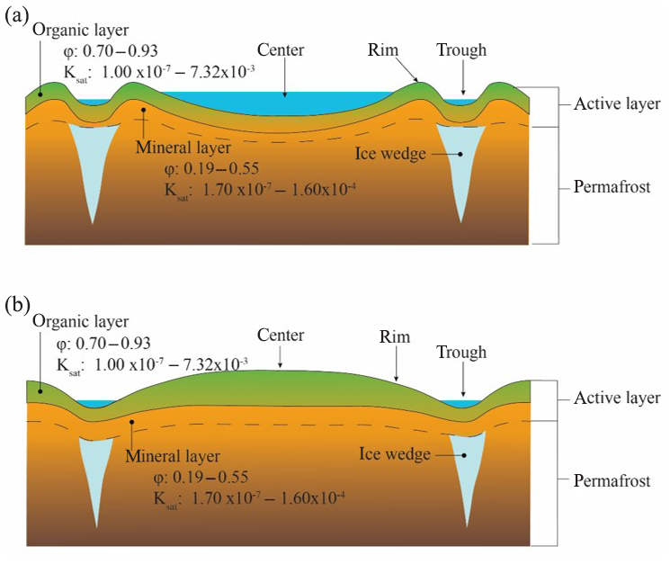
Figure 1Conceptual diagram of a low-centered polygon (a) and a high-centered polygon (b). Porosity and Ksat (m s−1) values from the literature (see Supplement, Table S1: Atchley et al., 2015; Beringer et al., 2001; Hinzman et al., 1991; Lawrence and Slater, 2008; Letts et al., 2000; Nicolsky et al., 2009; O'Donnell et al., 2009; Price et al., 2008; Quinton et al., 2000; Zhang et al., 2010).
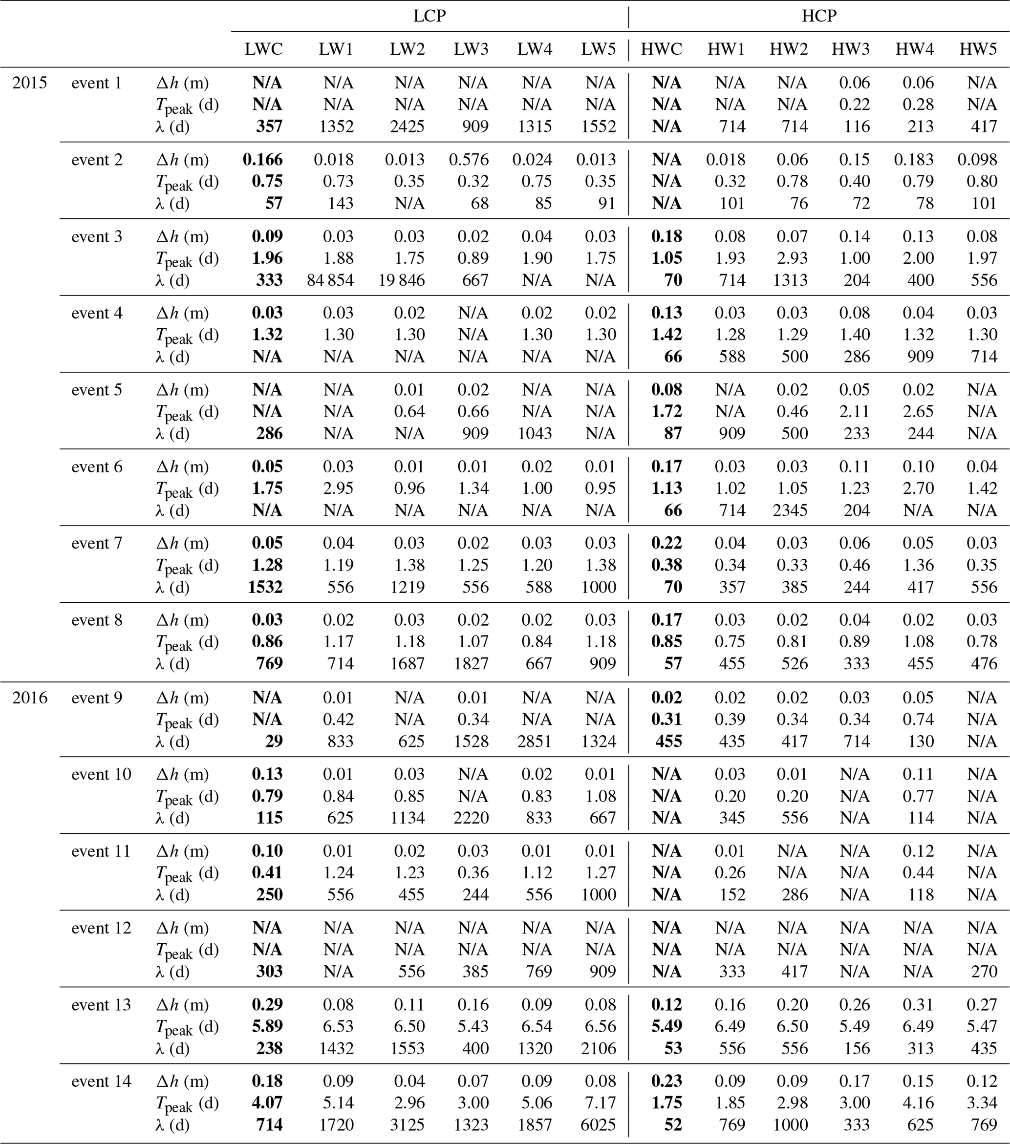
Table 1Response and recovery data from observation wells. Bold font indicates wells in polygon centers. Change in head Δh (m), time to peak Tpeak (d), and characteristic response λ (d). N/A = not available; the data necessary to make this estimate was not available.
It is now established that significant hydrological and biogeochemical differences exist on the sub-meter scale and are influenced by ice-wedge polygon type and microtopographic features (Andresen et al., 2016; Lara et al., 2015; Liljedahl et al., 2016; Newman et al., 2015; Wainwright et al., 2015). Permafrost degradation has the potential not only to change microtopographic features of ice-wedge polygons, but their hydrologic regimes as well. Understanding hydrologic regimes can help determine the fate of organic matter and nutrients in these landforms. For example, whether organic matter is decomposed into carbon dioxide or methane is largely determined by local hydrology.
Many studies have focused specifically on ice-wedge polygons, (e.g., Boike et al., 2008; Heikoop et al., 2015; Jorgenson et al., 2010; Lara et al., 2015; Newman et al., 2015) and provided much needed conceptualization (Helbig et al., 2013; Liljedahl et al., 2016). However, to our knowledge, few studies have been focused on quantifying the difference in relative roles of subsurface horizontal fluxes between low- and high-centered polygons, or characterizing heterogeneity of subsurface flow and transport within these landforms. Furthermore, most regional and pan-Arctic land models ignore horizontal flux and focus only on the representation of vertical water fluxes in the form of infiltration and evapotranspiration (Chadburn et al., 2015a, b; Clark et al., 2015). There exists a need to better quantify the relative roles of vertical and horizontal subsurface water fluxes in these landscapes, providing insight and data to revise, test, and calibrate permafrost hydrology representations in these models.
To this end, a tracer study was conducted on polygonal ground in the Barrow Peninsula of Alaska from July 2015 to September 2016. The Barrow Peninsula is located on the Arctic Coastal Plain adjacent to the Arctic Ocean. Approximately 65 % of the land cover in the Barrow Peninsula is ice-wedge polygonal ground, making this an ideal place to study the hydrology of ice-wedge polygons (Bockheim and Hinkel, 2010). To the best of our knowledge, and with the exception of an invasive and localized dye tracer experiment (Boike et al., 2008), this is the first non-invasive tracer study to be conducted at the polygon scale. Furthermore, this experiment is unique in that a tracer was continually monitored simultaneously on both a low- and high-centered polygon throughout thaw seasons, making it possible to characterize the breakthrough curves and determine times of first arrivals. Therefore, our approach permits a comparison of behaviors in low- and high-centered polygons over the same time period and meteorological conditions.
The purpose of this paper is to examine how differently low- and high-centered polygons behave hydrologically and to evaluate the relative importance of vertical and horizontal flux within polygon systems (including the controls of the frost table and microtopography on subsurface hydrology). The presence of significant horizontal flow can guide new upscaling approaches to incorporate these landscape features into regional hydrologic and biogeochemical models, which traditionally conceptualize the subsurface flow within ice-wedge polygons as exclusively vertical (Chadburn et al., 2015b; Clark et al., 2015). Insights from this study are intended to inform future work on the possible effects of permafrost degradation by improving the conceptualization used in the Arctic Terrestrial Simulator, developed by the Department of Energy at Los Alamos National Laboratory (Atchley et al., 2015; Painter et al., 2016) The Arctic Terrestrial Simulator performs calculations at the polygon scale and scales up to a watershed scale. Our primary focus is the hydrology of the active layer, which is the portion of the soil profile that thaws each year (Hinzman et al., 1991), with some emphasis on surface water. Possible mechanisms of flow heterogeneity are also discussed.
2.1 Site description
The study site is located east of Utqiaġvik (formerly Barrow), AK, USA, on the Arctic Coastal Plain in the Barrow Environmental Observatory (Fig. 2). The climate of this region is characterized by long winters and short summers, with a mean average annual temperature of −10.2 ∘C, and mean annual precipitation of 141.5 mm (NOAA-NCDC, 2000–2016). The coldest temperatures occur in February with warmest temperatures in July (NOAA-NCDC, 2000–2016). The thaw season usually begins in June with maximum thaw depth occurring sometime in late August or early September. Freeze-up typically begins sometime in September, subsequently leaving the ground completely frozen until June when the next thaw season begins. After the brief snowmelt period, a receding water table despite precipitation indicates that evapotranspiration dominates during the first half of the thaw season while a rising water table with precipitation indicates that precipitation and infiltration dominate during the second half of the thaw season. These observations are consistent with observations of evapotranspiration during the 2 years prior to the tracer experiment described here (Raz-Yaseef et al., 2017) and in other previous studies on Arctic water balances (Helbig et al., 2013; Pohl et al., 2009).
The region is characterized by low-relief land forms underlain by continuous, perennially frozen permafrost > 400 m thick and an active layer depth ranging from 30 to 90 cm (Hinkel et al., 2003; Hubbard et al., 2013). The soil profile consists of an organic layer typically < 40 cm thick underlain by a silty mineral layer composed primarily of quartz and chert (Black, 1964; Hinkel et al., 2003). The volume of shallow ground ice in the region can be as high as 80 % and is comprised primarily of ice wedges and cryogenic structures (Kanevskiy et al., 2013). Patterns of cryogenic structures found in frozen soils can result in higher porosities than found in unfrozen soils (Dafflon et al., 2016).
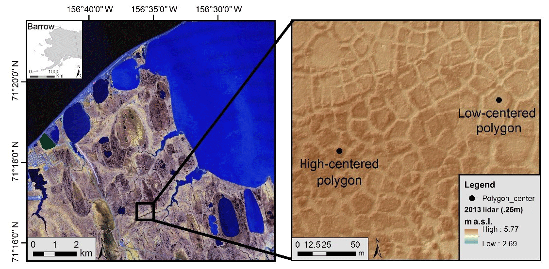
Figure 2Map showing the portion of the Barrow Peninsula where the study was conducted (left) and a close-up of the area containing the low- and high-centered polygons used for the tracer study.
One high-centered polygon (with an area of 132 m2) and one low-centered polygon (with an area of 706 m2) were chosen to reflect the extremes of tundra polygon morphology (Fig. 3). Only two polygons were used to minimize anthropogenic perturbations to the study site and because the cost and logistical complexity of these experiments is significant. Even though this limits our ability to replicate the results, the polygons selected are representative of a larger inventory of low- and high-centered polygons being investigated by our team at this intensive study site and have similar size and morphology, providing new insight into hydrologic differences between polygon types and into flow and transport across polygon features. The general soil profile of the polygons was an organic layer, comprised of 2–20 cm moss and peat (Iversen et al., 2015), underlain by a seasonally thawed mineral soil layer, followed by permafrost (Fig. 1). Ice lenses can form during freeze-up, especially in the mineral soil.

Figure 3Digital elevation model for the low-centered (a) and high-centered (b) polygons. Red dots represent locations of sampler nests and blue dots represent locations of observation wells. Blue circle indicates area of tracer application and encompasses the polygon center: 167.4 m2 for the low-centered polygon and 41.6 m2 for the high-centered polygon. Note scales are different for the two polygons.
2.2 Observational network
Each polygon had been instrumented with six fully screened observation wells (3.81 cm diameter PVC casing), one in the center of the polygon and five distributed along the surrounding troughs (blue circles in Fig. 3). All well casings were surveyed using a dGPS unit. Pressure transducers (Diver, Schlumberger Water Services, Netherlands) were deployed in each well to measure stage fluctuations at 15 min intervals and used to estimate water table elevations relative to ground surface (measured in meters above sea level, m a.s.l.). Barometric data were also collected at the study site and used to correct water level data for barometric effects. The pressure transducers have an accuracy of ±0.5 cm of H2O and a resolution of 0.2 cm of H2O.
To prevent preferential flow along the well casings, 15.24 cm diameter PVC pipe was placed around each well casing and pressed through the organic layer into the top 2 cm of the mineral layer (Fig. 4a). Silicon sheets 30.5 cm × 30.5 cm × 0.24 cm with pre-cut holes were also placed around each 15.24 cm pipe at the ground level to form a watertight seal. Additional silicon sheets of the same dimensions were placed around the samplers (discussed below) to prevent preferential or wall flow along the outer casing of the samplers. Caps were also placed on samplers between sampling events to prevent precipitation from collecting inside the housing of the samplers and diluting samples. Precipitation was measured using a tipping gauge rain bucket, 65 m from the study site.
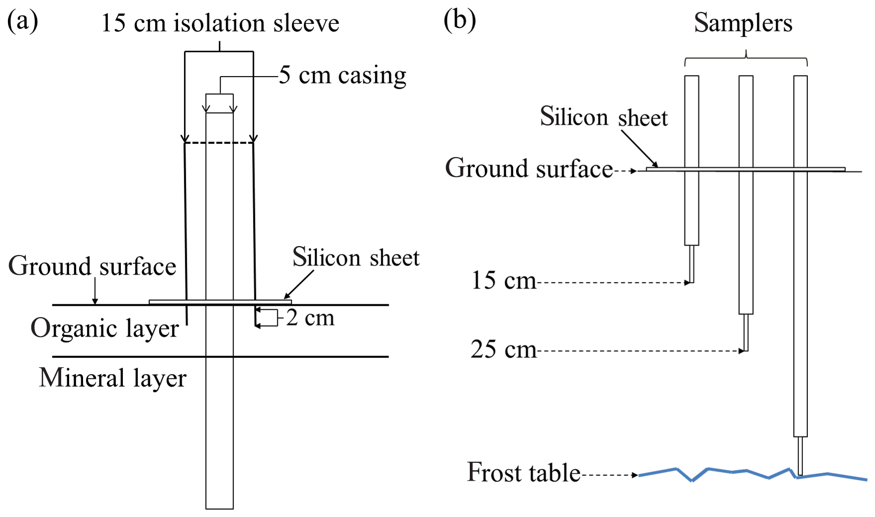
Figure 4(a) Schematic representation of the observation wells with isolation sleeve and (b) a schematic representation of a Rhizon sampling nest.
MacroRhizon samplers (Rhizosphere Research Products, Netherlands) were used to sample pore water at various locations and depths in both study sites (Fig. 4b). These samplers minimize perturbations to the porous media matrix and flow field by collecting sample volumes at low rates, no greater than 60 mL d−1, driven by the suction of a syringe at the surface. In addition, the sampler dimensions made it feasible to simultaneously sample three soil depths within a 12 cm diameter circle. Each sampler collected water through a tip 9 cm in length and 4.5 mm diameter with a mean pore size of 0.45 µm. In this work, sample depths refer to the insertion depth of sampler tip ends (Fig. 4b). In most cases, syringes remained on the samplers overnight to collect sufficient sample volumes, and therefore some sampling periods spanned over 24 h. When freezing temperatures were expected overnight, sampling was initiated and collected on the same day.
The rims of each polygon had eight nests of MacroRhizon samplers oriented in a radial pattern around the polygon (Fig. 3). Each sampler nest had samplers at three depths: 15 cm, 25 cm, and at the frost table. Samplers at the 15 and 25 cm depths were fixed over time while the deepest sampler, installed once the frost table reached a depth of 35 cm, was moved downward on a weekly basis as the frost table depth increased. Troughs surrounding each polygon also had eight nests of samplers adjacent to corresponding sampler nests on the rims (Fig. 3). Three nests of samplers were placed in the center of the low-centered polygon and only one in the center of the high-centered polygon due to its smaller relative area. Unlike the sampling nests in rims and troughs, samplers in polygon centers were inserted at 45∘ so the sampling tips would protrude past the edges of the silicon sheets. Samplers in polygon centers were inserted to depths of 15 cm and 25 cm, and frost table depth was sampled at 35 cm and deeper (Fig. 4b). An additional sampler nest was placed in the rim of the low-centered polygon where a saddle occurred, constituting an area of interest due to possible flow convergence. To minimize perturbations and avoid the generation of preferential flow paths, samplers at frost table depth were not removed prior to freeze-up at the end of the 2015 thaw season. As a result, in 2016, the deepest samplers were not sampled until the frost table reached the deepest depth for 2015.
2.3 Bromide tracer test
Bromide was used as a tracer due to its conservative nature with low potential for adsorption and ion exchange and negligible background concentrations (Davis et al., 1980). Other tracers were considered, but low background levels of bromide had been previously established (Newman et al., 2015), and given the high organic matter content and low pH of active layer waters, bromide was thought to be the best option. Potassium bromide (KBr) was dissolved in water and applied to the interior of each polygon with a garden sprayer (167.4 m2 for the low-centered polygon and 41.6 m2 in the high-centered polygon: outlined in blue in Fig. 3). A reference grid of nylon cord was used to guide the even distribution of tracer, and disposable rubber booties and latex gloves were worn during application to prevent contamination outside of the application area. A total of 8 L of tracer solution with a concentration of 5000 mg L−1 (40 g of Br) was applied to the high-centered polygon on 12 July 2015 and 24 L of tracer solution with a concentration of 10 000 mg L−1 (240 g of Br) was applied to the low-centered polygon on 13 July 2015. The higher concentration and volume used in the low-centered polygon compensated for the surface area, about 3 times larger than the high-centered polygon. A total of 10 L of water was subsequently sprayed on each polygon to facilitate infiltration of tracer into the soil.
2.4 Sampling and analytical methods
Sampling frequency in the MacroRhizon samplers varied depending on precipitation events and observed tracer concentrations. In 2015, samples were typically taken every 2 and 4 d during periods with and without precipitation events, respectively. We sampled daily during periods of persistent daily precipitation events. A full suite of samples was taken prior to tracer application to establish background levels of bromide. Pre-deployment bromide concentrations were consistent with those previously observed in the area (Newman et al., 2015), and many pre-deployment concentrations were at or near the limit of detection of the ion chromatograph used for analysis (0.01 ppm). In addition to groundwater samples, grab samples of surface waters were also collected during each sampling event. Samples were frozen and shipped to the Geochemistry and Geomaterials Research Laboratory (GGRL) at Los Alamos National Laboratory (LANL) for analysis. Samples were thawed and filtered through a 0.45 µm syringe filter prior to analysis via ion chromatography with an uncertainty of ±5 %.
Frost table depth measurements, taken with a tile probe, were typically taken weekly to the nearest 0.5 cm at each sampler nest. This served the dual purpose of ensuring the deepest sampler was at the depth of the frost table and measuring frost table depth. In both polygons, the frost table generally reached its deepest point in the beginning of September. Within the low-centered polygon, the maximum frost table depth measured over the two thaw seasons was 43 cm in the center, 45 cm in the rims, and 50 cm in the troughs. The maximum measured frost table depths for the high-centered polygon were 45 cm in the center, 43.5 cm in the rims, and 38 cm in the troughs for both field seasons.
2.5 Ground-penetrating radar
Ground-penetrating radar (GPR) surveys were conducted on each polygon to understand the influence of frost table topography on flow (Dafflon et al., 2015). GPR has been used for various applications in Arctic regions including estimation of thaw layer thickness (Bradford et al., 2005; Hubbard et al., 2013), characterization of permafrost and ice-wedge structure (Léger et al., 2017; Munroe et al., 2007), and mapping of snow thickness (Wainwright et al., 2017). In this study, common-offset surface GPR transects were collected on 2 October 2015 to estimate thaw layer thickness at the low- and high-centered polygon locations. GPR data were collected using a Mala Ramac system with 500 MHz antennas along four ∼34 m long parallel transects crossing the low-centered polygon, and along 51 ∼15 m long SE-NW transects spaced 0.25 m apart crossing the high-centered polygon. A wheel odometer was used to acquire traces with a spacing of 0.06 m. Minimal processing of the common offset lines included zero-time adjustment, bandpass filtering, automatic gain control, semi-automated picking of the two-way travel time to the key reflector, and conversion of travel time to depth. The key reflector corresponds to the interface between the thaw layer and the permafrost, as confirmed by the strong relationship between the GPR signal travel time and manual probe-based measurements of thaw layer thickness (correlation coefficient ∼0.73). The relationship has been used to convert the GPR signal travel time to thaw layer thickness. Frost table elevation was obtained by subtracting the GPR-inferred thaw layer thickness from the digital elevation model of the study site. Given the high spatial density of GPR data at the high-centered polygon location, a frost table elevation map was obtained through linear interpolation.
2.6 Core analyses
Shallow cores were extracted, using a SIPRE auger, from areas adjacent to the polygon tracer studies. Each core was collected from the frozen active layer at a different location. Cores were 46 mm in diameter and the lengths varied. Cores were kept frozen and, a few days after drilling, transported frozen to Lawrence Berkeley National Laboratory (LBNL) in Berkeley, CA. Three-dimensional images of the cores were obtained using a medical X-ray computed tomography (CT) scanner at 120 kV. Images were reconstructed to resolutions of 2.56 pixels per millimeter or better in the core-horizontal plane and 0.625 mm along the core-vertical axis. Additional cores containing ice lenses were extracted from the frozen active layer using a 51 mm diameter AMS soil auger. Cores were kept frozen until subsampling at the Permafrost Laboratory at the University of Alaska Fairbanks.
2.7 Well response and recovery
To better understand the response of the polygons to precipitation inputs, we focused on the temporal characteristics of water level changes caused by 14 precipitation events occurring over the 2015 and 2016 thaw seasons (Fig. 5). Each of these events is preceded and followed by relatively dry periods, resulting in water level changes with clear ascending and recovery curves. Isolating the water level hydrograph associated with each precipitation event allowed us to estimate the maximum change in head (Δh), time-to-peak (Tpeak), and characteristic recession time (λ) (Table 1). The characteristic recession time is calculated as the reciprocal of the slope for the line fitted to the natural log of water table elevation versus time during the recession limb. This recession time is a simple measure of the memory of the well to perturbations caused by precipitation events (Troch et al., 2013).

Figure 5Precipitation events, from 3 July 2015 to 30 September 2016, used in the calculation of characteristics of well response. Note that event 12 is not a precipitation event, but marks where a recession limb was analyzed for each well.
2.8 Tracer arrival and hydraulic conductivity
The temporal evolution of tracer concentrations at selected observation wells was used to approximate average linear velocities and bulk hydraulic conductivity values for each polygon. To this end, velocities were estimated by assuming that the transport of the tracer within the polygons can be approximated as a one-dimensional advective–dispersive problem with adsorption effects – a reasonable assumption given the lack of information and uncertainty in the spatial distribution of hydraulic parameters. This is a parsimonious approach to explore the first-order factors controlling fate and transport and timescales within this complex system. Van Genuchten and Alves (1982) found an analytical solution to this problem for the case of a semi-infinite soil profile without production or decay and with a constant initial concentration:
with
and initial and boundary conditions given by
In Eqs. (1) and (2), Ci (mg L−1) is initial concentration, Co (mg L−1) is input concentration, t (h) is time, to (h) is duration of solute pulse, and x (cm) is the lateral distance from the sampling nests to the edge of the tracer application area. The function A(x,t) is the effluent concentration, where R is the retardation coefficient (–), v is pore-water velocity (cm h−1), and D (cm2 h−1) is the dispersion coefficient.
We use the conditions in the field experiment to parameterize Eqs. (1) and (2). Background concentrations and tracer application varied for each polygon (see Table 2). In the high-centered polygon, the background concentration was Ci=0.19 mg L−1, and a solution with concentration Co=5000 mg L−1 was injected over a period of to=4.5 h. On the other hand, the low-centered polygon had a background concentration of Ci=0.44 mg L−1 and a solution with Co=10 000 mg L−1 was injected over a period of to=1.75 h. The dispersion coefficient was constrained to the range 1–100 cm2 d−1 based on the information available in Fig. 1 and Eq. (3) from Gelhar et al. (1992). With an average pH of 5.6 in the study area (Newman et al., 2015), the retardation factor was approximated as R=1.56 (Korom, 2000) – a reasonable value given the pH in Korom's experiment was between 5.1 and 5.7. Finally, arrival time (t=ta) for each sampler was determined by linear interpolation between the first breakthrough above background level (Ci). These times and the parameters specified above were used to approximate linear velocities and bulk hydraulic conductivity values for each polygon.
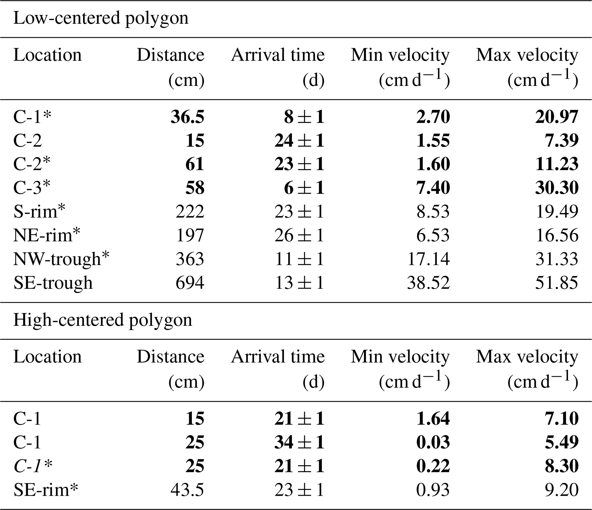
Table 2Tracer breakthrough locations, times, and linear velocities. Italic text indicates uncertainty in tracer arrival time due to insufficient data for interpolation. The * symbol denotes samplers at frost table depth. Bold font denotes vertical flow (center wells) and normal font denotes horizontal flow.
Consistent with the experiment, the arrival time for a sampler located at a distance x=L is significantly larger than the duration of tracer application, ta≫to, warranting the approximation and reducing Eq. (1) to the following:
Substituting Eq. (2) and rearranging, we obtain the following:
Then, the velocity v is estimated as the root of Eq. (4) (see Table 2) and assumes full saturation. Note that other approaches based on the center of mass of the breakthrough curve have been previously proposed (Feyen et al., 2003; Harvey and Gorelick, 1995; Mercado, 1967); however, they cannot be used in our experiment because only a small fraction of the tracer was recovered after 2 years of monitoring and the complete flushing of the tracer is likely to take several more.
Bulk hydraulic conductivities were then estimated using the fitted velocity values (Table 2). Vertical velocities were estimated by substituting L for the depth of the sampler. Horizontal velocities were estimated by substituting L for the shortest horizontal distance from the samplers in rims or troughs to the area of tracer application in the polygon interior. When estimating horizontal velocities, vertical arrival times could not be separated from the horizontal arrival times. Thus, resultant estimates for horizontal hydraulic conductivity were low bounding estimates.
Darcy's law was used to constrain hydraulic conductivity:
where Kh is the horizontal estimate of hydraulic conductivity, vh is the horizontal estimate of pore velocity, θ is effective porosity, Lh is horizontal distance, and Δh is the hydraulic head change. Ranges of Kh for each polygon were estimated using maximum and minimum estimated horizontal velocities and the minimum and maximum values of mineral layer porosity reported in the literature, 0.19 and 0.55, respectively (Beringer et al., 2001; Hinzman et al., 1998; Lawrence and Slater, 2008; Letts et al., 2000; Nicolsky et al., 2009; O'Donnell et al., 2009; Price et al., 2008; Quinton et al., 2000; Zhang et al., 2010). The change in hydraulic head was estimated by finding the average head difference, over the course of observation in 2015, between the well in the polygon center to the well nearest the sampler of interest.
2.9 Mass balance
While it was not possible to close the mass balance of the tracer without compromising the experiment (i.e., by coring or digging pits) an attempt was made to bracket the mass balance. For each polygon, the largest and smallest breakthrough curves via horizontal flux were used to estimate the limits at which horizontal flux had redistributed tracer from polygon centers to rims and troughs. Only one breakthrough curve was used for the high-centered polygon since breakthrough was only detected at one location outside the polygon center. First, each polygon was idealized as a cylinder and its area calculated so flux could be estimated. The radius used for the idealized cylinder of the low-centered polygon was 13.4 m and the radius used for the high-centered polygon was 3.8 m. Second, flux was calculated through the side of the cylinder as the product of the area, porosity, and velocity. Mineral layer porosity values of 0.19 and 0.55 were used, representing the minimum and maximum porosity values listed above, and the values used for velocity were the previously mentioned linear velocity values. Lastly, the product of the flux and change in tracer concentration over time were integrated with respect to time.
3.1 Flow characteristics (observations)
From the beginning of July until mid-August in each thaw season (2015 and 2016), there was relatively little precipitation in the study area and the water table was receding (Figs. 6 and 7). In both thaw seasons, most of the precipitation occurred between mid-July and the end of August, concurrent with a rising water table. This behavior is explained by evapotranspiration dominance during the first half of each season, previously observed by Raz-Yaseef et al. (2017), and infiltration dominance in the second half. Daily average temperatures fluctuated between −0.7 and 7.8 ∘C and −1.7 and 13.7 ∘C in the 2015 and 2016 thaw seasons, respectively (NOAA-CRN 2015-2016). We observed that the study site was much drier in the 2016 thaw season, with far less standing water in the study area than in the 2015 thaw season. In addition, overland flow was never observed as a result of precipitation events, suggesting high infiltration capacity and dominance of subsurface flow.
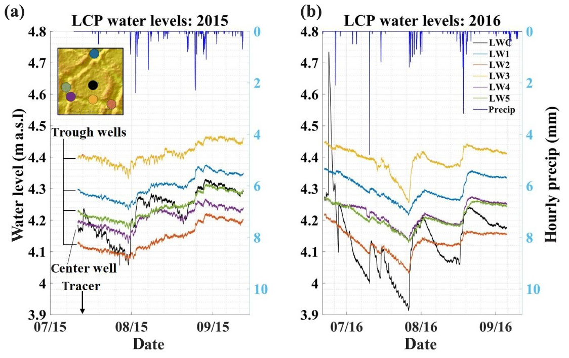
Figure 6Water levels from the low-centered polygon (LCP) for the 2015 (a) and 2016 (b) thaw seasons. Arrow indicates date of tracer application. Dots in the inset (upper-left) correspond to observation-well locations; colors of the dots correspond to well hydrographs. Dark blue lines along the top of the graphs indicate hourly total precipitation.
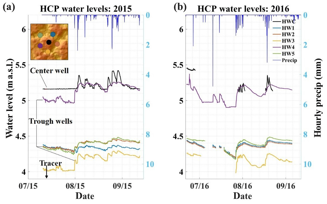
Figure 7Water levels from the high-centered polygon for the 2015 (a) and 2016 (b) thaw seasons. Dots in the inset (upper-left) correspond to observation-well locations; colors of the dots correspond to well hydrographs. Dark blue lines along the top of the graphs indicate hourly total precipitation.
Water levels in the low-centered polygon varied less than 40 cm throughout both thaw seasons, with the exception of a peak in the center well in 2016 (Fig. 6) which is most likely from meltwater filling the well when the frost table was only a few centimeters deep. For much of the 2015 thaw season, the water level in the center well was as high as or higher than three out of five of the trough wells, indicating variable hydraulic gradients across the polygon. Conversely, for most of the 2016 thaw season, the water level in the center well was lower than the wells in the troughs, indicating the possibility of the reversal in the direction of the hydraulic gradient from the polygon center to troughs. Inspection of the well hydrographs reveals that the center well responded as quickly as trough wells to precipitation events, but with faster increases in water table elevation and steeper recession limbs.
In the low-centered polygon, most precipitation events resulted in higher Δh values in the polygon center than in trough wells while characteristic recession times, λ, in the polygon center were generally shorter than those of trough wells (Table 1). This is consistent with infiltration and ponding in the center of the polygon with subsequent subsurface horizontal redistribution of mounded groundwater to the troughs. When the system is low in storage (i.e., events 2–4) (Fig. 5 and Table 1), Tpeak values tend to be lower in trough wells than in the center well. Wells located in the troughs are in topographic lows acting as convergence areas where ponding is likely to occur (Fig. 3). Conversely, when the system is higher in storage (i.e., events 7 and 8), ponding occurs more quickly in the polygon center, resulting in Tpeak values in the polygon center that are shorter or more similar to those in the troughs. This behavior highlights the importance of microtopography and storage on flow within the low-centered polygon.
At the high-centered polygon, water levels between center and trough locations often varied by nearly a meter. The center well, HWC, was often dry in the 2016 thaw season as were trough wells HW1, HW2, HW3, and HW5 (Fig. 7). When the center well was not dry, the water level was typically higher than that of the trough wells, indicating a hydraulic gradient from the polygon center to the troughs when water was present. Inspection of the well hydrographs reveals that the well in the polygon center, HWC, had steeper post-precipitation recession limbs than wells in the troughs.
The high-centered polygon most often had higher Δh values in the polygon center than in the troughs. Additionally, recession times, λ, were usually shortest in the polygon center with longer times in the troughs. As in the low-centered polygon, this is consistent with groundwater mounding in the center with subsequent subsurface horizontal redistribution to the troughs. Of the trough wells, HW3 and HW4 tended to have the highest Δh values with shorter recession times, λ, than other trough wells (Fig. 7 and Table 1). Notice that these wells are located in high sections relative to the rest of the trough, but low relative to the polygon center. Further, the GPR survey of the high-centered polygon shows that, unlike surface topography, most of the frost table in the polygon center (the area within the tracer application zone outlined by the blue circle) slopes to the south-southwest (Fig. 8b). This indicates that the majority of mounded groundwater from the polygon center is likely redistributed to the south-southwest trough of the polygon at HW3 and HW4. Subsequently, mounded water at HW3 and HW4 is redistributed to other parts of the polygon trough. Conversely, HW1, HW2, and HW5 usually have smaller Δh, shorter times-to-peak, and longer recession times indicating that ponding is dominant in these areas (Table 1).
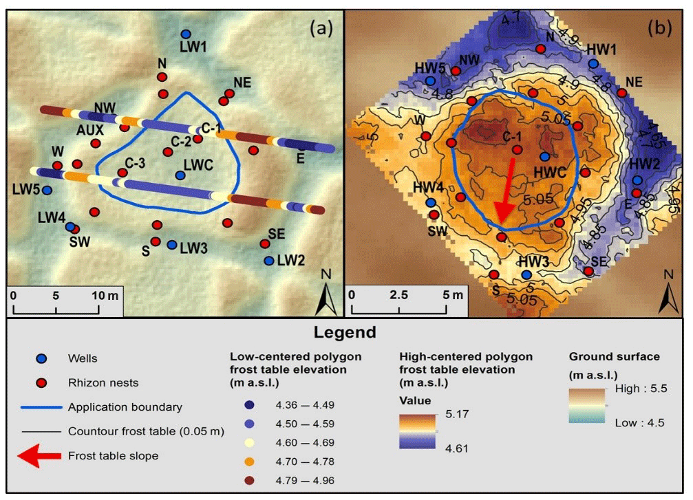
Figure 8Frost table elevation obtained with a ground-penetrating radar survey at the (a) the low-centered and (b) high-centered polygon locations. Note that transect lines indicate frost table elevation at the low-centered polygon (a) while topographic lines indicate frost table elevation at the high-centered polygon (b). Red arrow indicates the direction of frost table slope in high-centered polygon. Widths of transects on low-centered polygon exaggerated for legibility. See Supplement, Tables S2 and S3 for frost table depths.
3.2 Transport characteristics (observations)
Tracer breakthrough for both polygons did not exhibit smooth breakthrough curves typically seen in laboratory tracer experiments. Instead, these breakthrough curves have a more jagged form, showing sudden changes in concentration. This jagged nature is due partly to sampling frequency. Often, there were several days between sampling events, resulting in breakthrough curves with a low temporal resolution. However, there is also evidence that large rain events were responsible for some of this variability over time. For example, in the low-centered polygon, there was a concentration increase in well C-1 at the frost table after precipitation Event 3 (Figs. 5 and 9).
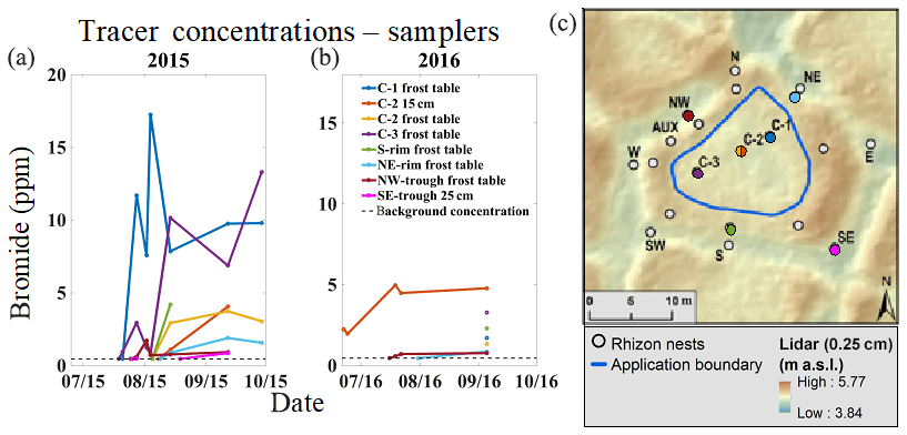
Figure 9Tracer breakthrough curves for the low-centered polygon (a) and dots representing their corresponding locations (c). The color of the dots correspond to the breakthrough curve of the same color. The blue line on the polygon digital elevation model (c) depicts the area of tracer application.
At the low-centered polygon, tracer arrived first at the center samplers, second in the trough samplers, and third at the rim samplers (Fig. 9 and Table 2). Tracer breakthrough in the center had higher concentrations than in rims or troughs. This was expected as the center was the area of tracer application. While the succession of vertical breakthrough was not entirely captured at all three depths for all three center sampling locations in the low-centered polygon, tracer arrival times were different for each sampling location in the center. Specifically, tracer arrived first at the frost table of the C-3 sampler after 6 d, then at the frost table of the C-1 sampler after 8 d, at the frost table of the C-2 sampler after 23 d, and finally at the 15 cm depth of the C-2 sampler after 24 d (Fig. 9 and Table 2). Linear velocities of vertical infiltration, calculated using the Eq. (4), varied from 1.55 cm d−1 at the 15 cm depth of the C-2 sampler to 30.3 cm d−1 at the frost line of the C-3 sampler (Table 2).
The tracer reached the northeast and southern rim locations and the northwest and southeast trough locations of the low-centered polygon (i.e., sampling outside the polygon center) via subsurface flow paths (Fig. 9). As previously mentioned, no overland flow was observed from polygon center to troughs. Interestingly, when tracer breakthrough was detected at trough locations, there was no breakthrough detected at their adjacent rim locations. In addition, all tracer breakthroughs in the rims and the troughs were detected at frost table depth except for the southeast trough location, which occurred at the 25 cm depth. This highlights the influence of the frost table topography.
Tracer was detected at the more distal trough locations of the low-centered polygon before it was detected at the relatively proximal rim locations. More specifically, tracer arrived first at the two trough locations after 11 and 13 d then at the two rim locations after 23 and 26 d. At the northwest and southeast trough locations, estimated horizontal linear velocities ranged from 17.1 to 31.3 and 38.5 to 51.8 cm d−1, respectively. At the northeast and southern rim locations, estimated horizontal linear velocities ranged from 6.53-16.5 cm d−1 and 8.53–19.5 cm d−1, respectively (Fig. 9 and Table 2). Using Eq. (5), the range of horizontal hydraulic conductivity based on first arrivals was estimated to be between and m s−1.
Tracer was also detected in surface water sampled from the troughs around the low-centered polygon. Samples collected during 2015 show an increasing trend in tracer concentration near the end of the season (Fig. 10b). Even though surface water tracer concentrations for 2015 were relatively low, several of the concentrations were above the 0.44 mg L−1 background level for bromide. This observation can be interpreted as an integrated, well-mixed response of all the tracer that was transported from the polygon center to the troughs via the subsurface. Surface water samples collected from troughs during 2016 did not show a clear trend of increasing tracer concentration (Fig. 10a).
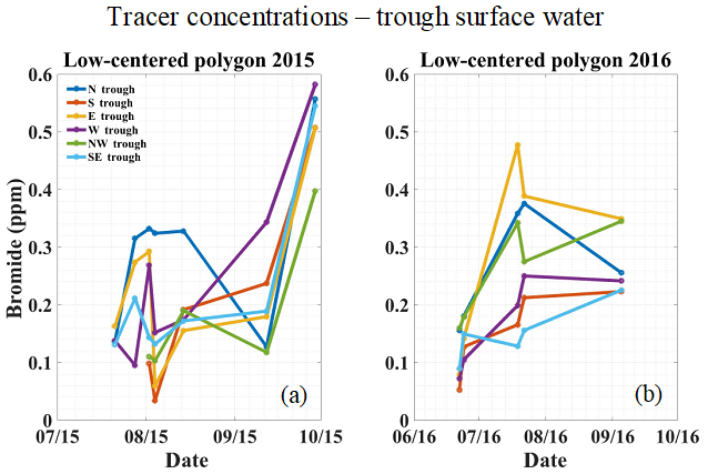
Figure 10Breakthrough curves sampled from the surface waters in polygon troughs for (a) low-centered polygon in 2015 and (b) low-centered polygon in 2016. Notice the upward trend in tracer concentration in the troughs of the low-centered polygon (a) during the 2015 thaw season.
At the high-centered polygon, tracer arrived first in the center (C-1) via vertical infiltration, and second in one rim location via subsurface horizontal flux (Fig. 11 and Table 2). The center location exhibited tracer arrival times that did not necessarily correlate with depth. That is, tracer first arrived simultaneously at the 15 cm and frost table samplers after 21 d, and second at the 25 cm sampler after 34 d. Linear velocities of vertical infiltration, calculated from arrival times, varied from 0.03 to 8.3 cm d−1.
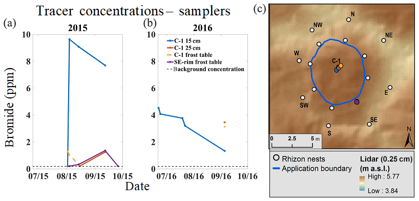
Figure 11Tracer breakthrough curves for the high-centered polygon (a) and dots representing their corresponding locations (c). The color of the dots correspond to the breakthrough curve of the same color. The blue line on the polygon digital elevation model (c) depicts the area of tracer application.
Horizontal tracer flux was evident in only one location outside the center of the high-centered polygon: the southeast rim location (Fig. 11 and Table 2). Tracer arrived at the frost table depth of this location after 23 d. Linear velocity, estimated using Eq. (4), was between 0.93 and 9.2 cm d−1. The range of horizontal hydraulic conductivity for the high-centered polygon was estimated to be between and m s−1. Overall, bromide concentrations in trough surface waters of the high-centered polygon were low. While there were only slight concentration increases (around 0.1 mg L−1) in three trough locations at the end of 2015, these concentrations indicate a very small breakthrough, if any.
While horizontal hydraulic conductivity estimates were higher for the low-centered polygon than for the high-centered polygon, there was only one estimate for the high-centered polygon. Unlike the low-centered polygon where tracer was applied to a relatively saturated surface, tracer was applied to a dry surface in the high-centered polygon. In both polygons, estimates of horizontal hydraulic conductivity are minimum estimates because vertical arrival times could not be separated from horizontal arrival times.
3.3 Mass balance
For the low-centered polygon, the largest tracer mass that could have left the polygon center was estimated to be 93.68 % of the tracer. This number is unrealistically high given that the breakthrough curve used in the estimate was incomplete and that the high bounding value used for mineral porosity was likely overestimated. The smallest tracer mass estimated to have left the center, based on the smallest breakthrough curve, was 4.80 %. This number can be considered a “maximum–minimum” and is likely an overestimate since tracer was not detected at all sampling locations around the polygon. For the high-centered polygon, the largest tracer mass that could have left the polygon center was estimated to be 6.82 % while the smallest estimated mass was 2.36 %. Again, this number can be considered a “maximum–minimum” since the tracer was not detected at all sampling locations around the polygon. Even though these estimates have large uncertainties, it appears that most of the tracer remains within the interior of both polygon centers.
The general pattern in tracer dynamics in both polygon types was to first infiltrate vertically until it encountered the frost table, then to be transported horizontally, highlighting the influence of the frost table on horizontal flux. There were no new tracer arrival locations during the 2016 thaw season beyond those identified in 2015. Only a small percentage of tracer mass was recovered after monitoring breakthrough over 2 years, indicating that subsurface flow and transport within both polygon types was very slow. Ranges of hydraulic conductivity estimated for both polygons fall within the range of vertical conductivity found in the literature (Atchley et al., 2015; Beringer et al., 2001; Hinzman et al., 1991, 1998; Lawrence and Slater, 2008; Nicolsky et al., 2009; O'Donnell et al., 2009; Price et al., 2008; Quinton et al., 2000; Zhang et al., 2010). However, assuming uniform values for horizontal conductivity is probably inappropriate as there were several rim and trough locations where no tracer was detected.
Overall, the low-centered polygon had higher fluxes and tracer breakthroughs at more locations than in the high-centered polygon. The observed differences in tracer flux between polygon types is, in part, explained by degree of saturation. The high-centered polygon, by its very nature, had a higher center relative to the water table and was drier than the center of the low-centered polygon. As a result, the tracer was applied to a more saturated surface on the low-centered polygon as opposed to a dry surface on the high-centered polygon. This allowed the tracer to become mobile more quickly in the low-centered polygon even though the elevation gradient was higher in the high-centered polygon.
4.1 Heterogeneity of flux and contributing factors
Both polygon tests demonstrate heterogeneity of vertical and horizontal tracer flux. Preferential flow paths or heterogeneity of subsurface media likely contribute to the heterogeneity of tracer transport observed in both polygon types. Evidence from cores, GPR data, and previous studies provides insight into factors that may be contributing to the heterogeneity of the flow system. The relative importance of these factors still needs to be established.
Results suggest heterogeneity in porous media characteristics affects vertical transport. Different arrival times at the frost table were observed in the low-centered polygon and various linear velocities were observed in the center of the high-centered polygon (Figs. 9, 11 and Table 2). These differences indicate preferential flow in the vertical direction and the existence of secondary porosity.
The wide range in horizontal hydraulic conductivity observed in both polygons is also characteristic of preferential flow paths or heterogeneous subsurface media. Within the low-centered polygon, tracer arrival in the two trough locations was not preceded by tracer arrival in adjacent rim locations (Fig. 9, Table 2). It seems that tracer was able to move to the trough through areas in between the rim sampler locations, at least in the early part of the experiment. For example, in the low-centered polygon, tracer arrived at the northeast trough location, but without ever arriving at the northeast rim location. This implies that flow paths exist that routed the tracer flux around the adjacent rim location to the corresponding trough location. In the high-centered polygon, the only breakthrough detected outside the polygon center was at the southeast rim location (Fig. 11), indicating heterogeneity in horizontal transport.
Characteristics of active layer soils help to explain heterogeneity of flux. For example, variability in vertical and horizontal flux is consistent with the soil structures observed in CT scans of cores taken from other ice-wedge polygons near the study area (Fig. 12a and b). Patterns of vertical and horizontal density contrasts throughout the cores reflect heterogeneity and dual porosity of the peat and mineral layers, indicating the potential for preferential flow. These patterns may also be indicative of partial melting or partial freezing of the soil profile as a driver of heterogeneous flow. Cryoturbation, a freeze–thaw process that mixes organic and mineral soils within the active layer (Bockheim et al., 1998; Michaelson et al., 1996), is also a potential cause of heterogeneity in subsurface media. Cryoturbation results in discontinuous, non-stratified soil horizons. Contrasts in hydraulic properties between discontinuously distributed soil types likely contributes to heterogeneity in flow and transport.
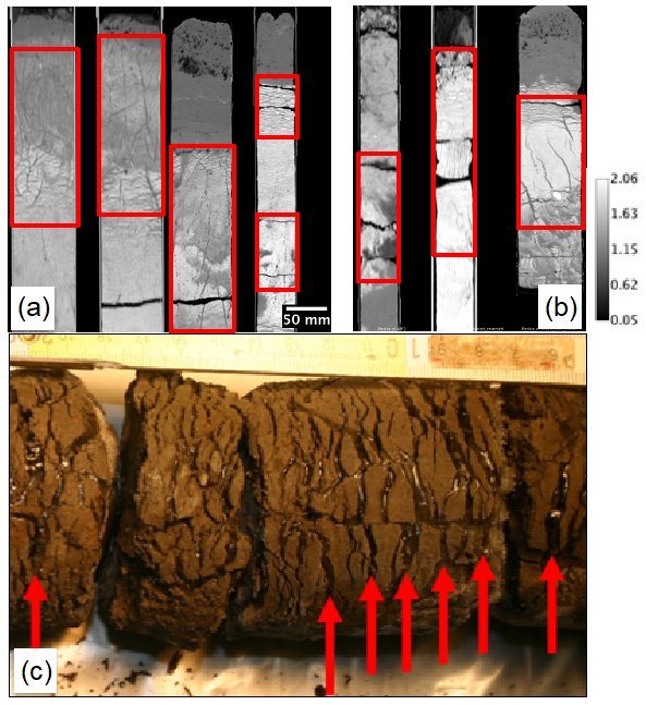
Figure 12Vertical cross sections of X-ray CT scans of the top 40 cm of cores from (a) low-centered polygons and (b) high-centered polygons. The CT scans show the density distribution from low (dark) to high (white) with a calibration bar shown in grams per cubic centimeter (g cm−3). Red boxes indicate patterns of vertical and horizontal density contrasts. Frozen core sampled from saturated tundra (c) is analogous to a low-centered polygon. Red arrows indicate prominent ice lenses. Ice lenses are formed at freeze-up when the soil is sufficiently saturated. Notice that most ice lenses are horizontal relative to ground surface. Photo credit: Vladimir Romanovsky.
The influence of frost table topography on horizontal flux is significant within both polygons. Outside of polygon centers, tracer was detected almost exclusively at the frost table. The structure of frost table topography can be seen through the GPR survey. The GPR transects at the low-centered polygon show the trend that frost table topography generally follows surface topography (Fig. 8). More specifically, higher-elevation frost table areas are overlain by higher-elevation surface topography and lower-elevation frost table areas are overlain by lower-elevation surface topography. Three of the four locations where tracer was detected outside the center of the low-centered polygon are where the surface topography, and therefore the frost table topography, is relatively low in the rim separating the polygon center and trough (Figs. 8 and 9). Low points in the topography of the frost table help to explain why breakthrough was detected in these locations. This observation is consistent with observations of low-centered polygons by Helbig et al. (2013) and studies of other Arctic landforms underlain by permafrost (Morison et al., 2017; Wright et al., 2009). Similarly, in the high-centered polygon, frost table topography within the application area slopes to the south-southwest and the only tracer breakthrough detected outside the polygon center was in the southern half of the polygon (Figs. 8 and 11).
The presence of ice lenses may also drive differences in subsurface horizontal flux between the low- and high-centered polygons. A frozen core, shown in Fig. 12c, was collected from saturated tundra at the Barrow Environmental Observatory. Although this core was not taken from the polygons used in this experiment, it can be used as an analog for understanding the effect of ice lenses in subsurface structure. In fully saturated tundra, such as the low-centered polygon, ice lenses tend to form during freeze-up whereas they are not as common where tundra is unsaturated, as in the high-centered polygon. This core, taken from a saturated area, exhibits ice lenses up to 3 mm wide primarily in the horizontal plane. These structures are consistent with those found in the transient layer as described by Shur et al. (2005). We speculate that, as the active layer progressively thickens each year and these ice lenses thaw, some of the resultant cracks remain open enough to create secondary porosity within the low-centered polygon. A system of secondary porosity, oriented primarily in the horizontal plane, helps explain why the low-centered polygon would exhibit faster tracer breakthrough in more rim and trough locations and at higher rates than the high-centered polygon. Whether or not these cracks stay open, and for how long, may be a function of soil structure. For example, cracks running through soil containing high concentrations of decomposed organic matter may collapse more quickly following thaw of ice lenses while cracks running through soil without decomposed organic matter remain longer. Variable collapse of secondary porosity structures across the polygon may help to explain heterogeneity of horizontal tracer breakthrough in rims and troughs. Furthermore, thicker and more numerous ice lenses tend to form at the bottom of the active layer, near the top of the permafrost (Guodong, 1983; Shur et al., 2005), helping to explain why most breakthrough was observed at the frost table. Additional research is needed to evaluate the importance of ice lenses on flow and transport within polygon systems.
4.2 Transition between 2015 freeze-up and 2016 thaw
It might be assumed that, due to freezing, tracer migration would resume in 2016 where it ended in 2015. However, in 2016, results show a substantial reduction in tracer concentration as compared to the end of the 2015 thaw season (Figs. 9–11). In fact, concentrations dropped by as much as 81 % and many locations with tracer breakthrough in 2015 did not experience tracer breakthrough until late in the 2016 thaw season. Since tracer was mostly detected at frost table depth in 2015, it would have been contained in the frozen subsurface at the start of the 2016 thaw season. This implies that tracer would not become mobile in the second year until the active layer thawed to the depth at which the tracer was frozen in the first year. Even when the ground thawed to depth of the tracer, the tracer could have been further diluted. That is, once the part of the soil profile containing tracer begins to thaw it could have also mixed with precipitation that had newly entered the system even before all the tracer-containing ground was thawed. Mixing with precipitation from the second year would cause the tracer to become further diluted and dampen the breakthrough response.
Redistribution of tracer in the soil horizon during freeze-up may have also been a factor in the reduction of tracer concentrations between the 2015 and 2016 thaw seasons. Tracer freeze-out could have contributed to tracer redistribution between thaw seasons. Freeze-out is a process by which, as freeze-up progresses, most of the tracer remains in the aqueous component. In the Arctic, the active layer freezes from the top down and the bottom up simultaneously (although not necessarily at the same rate) (Cable, 2016). Thus, the tracer could have been redistributed within the soil profile as a result of freeze-out while remaining mobile in the unfrozen portion of the soil profile until freeze-up was complete. It has also been established that temperature and vapor gradients have the potential to cause redistribution of soil moisture (Hinzman et al., 1991; Painter, 2011; Schuh et al., 2017). During freeze-up, cryosuction allows for soil moisture to migrate towards the freezing front. The freeze-out and cryosuction processes could have a combined effect on redistribution of the tracer within the active layer of the polygons.
Snowmelt at the beginning of the 2016 thaw season may have enabled the rapid removal of some tracer, especially from troughs. No samples were taken during snowmelt which typically lasts no longer than 2 to 3 weeks (Hinzman et al., 1991). A significant reduction in tracer concentration can be seen in the troughs of the low-centered polygon from the end of the 2015 thaw season to the beginning of the 2016 thaw season (Fig. 10a and b). Since these represent surface waters, the reduction in concentration here may be explained by snowmelt dilution and runoff. This phenomenon may not affect the subsurface because only a shallow portion of the soil profile is thawed during snowmelt.
Overall, the results suggest a conceptual model of how solutes are transported within ice-wedge polygons (Fig. 13). One early hypothesis was that a contrast in hydraulic properties between the organic and mineral layers would be a primary factor limiting vertical flux and promote lateral flux, which results did not corroborate. In both polygons, the role of the frost table proved to be more important in inhibiting vertical flux as tracer was transported vertically, then horizontally upon encountering the frost table. Results from GPR and well responses indicate that frost table topography also influences the heterogeneous horizontal distribution of solutes within polygon systems. Horizontal conductivity estimates suggest that, at the polygon scale, horizontal flux does play a role, although perhaps not to the same degree as vertical flux. Both polygons experienced breakthrough in the first thaw season, first in polygon centers via vertical infiltration, then outside of polygon centers at frost table depth via subsurface horizontal flux. Only a small percentage of tracer mass was recovered over 2 years of monitoring, indicating that flow and transport were very slow and that both polygons had a high residence time, with most of the tracer mass likely remaining in polygon centers.
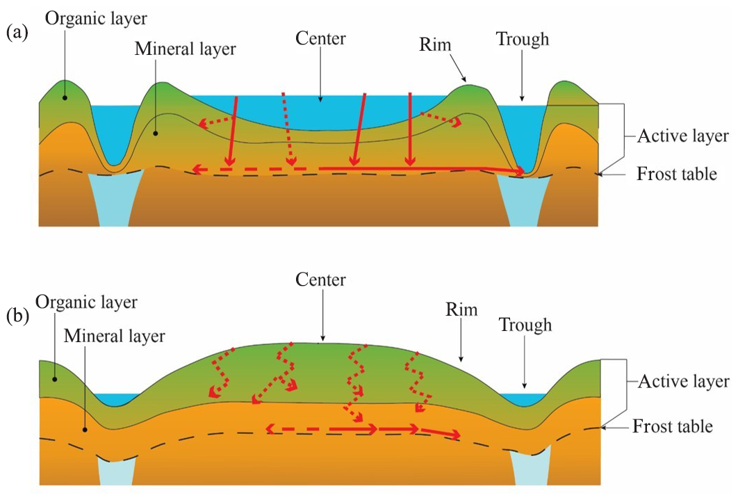
Figure 13Conceptual diagram of tracer transport in ice-wedge polygons. Red arrows indicate transport pathways. Length of arrow indicates relative flux. Dashed arrows indicate lower rates of flux than solid arrows.
Vertical and horizontal flux proved to be highly heterogeneous in both polygon types. Heterogeneity in vertical flux manifested in both polygons as tracer arrival at deeper depths before arriving at relatively shallow depths at a given location. Heterogeneity in subsurface horizontal flux for both polygon types is demonstrated by the fact that tracer arrived at only 4 out of 17 sampler nests outside of the center in the low-centered polygon and only 1 out of 16 sampler nests outside of the center in the high-centered polygon. Tracer arrival times and estimates of horizontal conductivity in the low-centered polygon also show significant variability.
Besides the arrival of tracer outside of polygon centers, the existence of subsurface horizontal flux was also supported by the characteristic responses of observation wells within both polygons. Well responses indicated that water from polygon centers was redistributed to polygon troughs after rain events. Also, there were no observations of overland flow during the course of the entire experiment, even during multi-day rain events. This implies that, in both low- and high-centered polygons, all flow from the center to the troughs took place in the subsurface. In the low-centered polygon, tracer found in surface water of troughs also supports the existence of subsurface horizontal flux.
While subsurface horizontal flux did play a role in both polygon types, results suggest that the low-centered polygon experienced higher subsurface horizontal flux in more locations than the high-centered polygon. Furthermore, estimates of hydraulic conductivity in the low-centered polygon were orders of magnitude higher than in the high-centered polygon. The degree of saturation may explain why the low-centered polygon experienced higher subsurface horizontal flux. Saturated media probably allowed for more immediate mobilization of the tracer in the low-centered polygon. The formation of ice lenses in the low-centered polygon is another possible explanation of the increased horizontal conductivity due to secondary porosity.
Even though temporal changes are not shown in Fig. 13, temporal aspects are an important part of the conceptual model. For example, while the changing elevation of the frost table and its topography is not depicted, it plays an important role in inhibiting infiltration and influencing preferential flow. Similarly, the transition between winter freeze-up and subsequent thaw also has a significant effect on tracer transport.
This conceptual model has implications for biogeochemical processes. Distinct biogeochemical differences have been shown to exist between different microtopographic features of polygons (Andresen et al., 2016; Lara et al., 2015; Liljedahl et al., 2016; Newman et al., 2015; Wainwright et al., 2017; Zona et al., 2011b). These tracer results suggest there are lateral connections between polygon centers and troughs that can facilitate transport of chemical species across microtopographic features. This transport could affect redox conditions and have multiple effects on biogeochemical cycling. For example, water in the centers of high-centered polygons has been shown to have significantly higher concentrations of nitrate and sulfate than water in the troughs (Heikoop et al., 2015; Newman et al., 2015). When water in the center of a high-centered polygon is redistributed to the polygon trough, due to preferential pathways, it could cause oxyanions to be transported to the troughs in a heterogeneous manner. In turn, this may influence carbon partitioning by influencing microbial respiration and plant growth (Weintraub and Schimel, 2005; Zona et al., 2011b). As a result, models including horizontal flux may represent carbon partitioning and the migration of plant communities more accurately than models that assume only vertical flux is relevant.
Our study provides new insight into hydrological processes of low- and high-centered polygon systems, where flow and transport field investigations are almost totally lacking. This study shows that polygon type significantly affects flow and transport as faster and more prolific tracer breakthrough was observed in low-centered polygons than high-centered polygons, confirming speculation by other researchers. Results suggest that horizontal flow is important, and that heterogeneity of subsurface media plays a significant role in flow and transport. Our study also provides some evidence about what is potentially controlling heterogeneity. These insights can help to improve hydrological models such as the Arctic Terrestrial Simulator, a full energy balance model being developed to simulate flow and transport at the individual polygon level (Atchley et al., 2015; Painter et al., 2016).
Given that much of the tracer remains in the polygons, longer-term monitoring of at least 5 years would contribute to a better understanding of these systems. Future tracer studies of this kind should consider that multi-year sampling will likely be necessary to adequately capture complete breakthrough curves. Such an experiment would highlight the importance of interseasonal variations. Additional work is also needed toward understanding controls on the heterogeneity of flux in ice-wedge polygons; for example, the effect of ice lenses and cryoturbation on flux require further investigation.
Data sets are available on request at the NGEE-Arctic data repository (Wales et al., 2020; https://doi.org/10.5440/1342954).
The supplement related to this article is available online at: https://doi.org/10.5194/hess-24-1109-2020-supplement.
BDN originally conceived of the experiment and NW and CJW helped to refine the experimental design. NAW performed the majority of field work and data analysis and wrote the paper. BD performed the GPR survey of the study site. TJK collected frozen cores and conducted CT scans. JDGV provided contributions to the design and implementation of the data analysis approach and helped with the writing of some sections, including the results. CJW and SDW provided institutional oversight. All authors provided comments and text prior to the submission of the paper.
This work has been authored by an employee of Los Alamos National Security, LLC, operator of the Los Alamos National Laboratory, under contract DE-AC52-06NA25396 with the US Department of Energy.
This work was supported by the DOE Office of Science, Biological and Environmental Research program and the Next Generation Ecosystem Experiment (NGEE-Arctic) project. We are grateful to George Perkins, Emily Kluk, and the staff of the GGRL at Los Alamos National Laboratory for their work in sample analysis. We thank Anna Liljedahl for early contributions to experimental design and for the use of preexisting infrastructure. We also thank Lauren Charsley-Groffman for GIS work and her work in the field. We thank John Peterson for helping GPR data acquisition and processing. We acknowledge Vladimir Romanovsky for his pictures of frozen cores and Bob Busey for the use of his meteorological data.
This research was undertaken by the Los Alamos National Laboratory under contract to the Department of Energy (contract number DE-AC52-06NA25396).
This paper was edited by Theresa Blume and reviewed by two anonymous referees.
Andersland, O. B., Ladanyi, B., and ASCE: Frozen Ground Engineering, 2 edition, Wiley, Hoboken, NJ, Reston, Va, 2003.
Andresen, C. G., Lara, M. J., Tweedie, C. E., and Lougheed, V. L.: Rising plant-mediated methane emissions from arctic wetlands, Glob. Change Biol., 23, 1128–1139, https://doi.org/10.1111/gcb.13469, 2016.
Atchley, A. L., Painter, S. L., Harp, D. R., Coon, E. T., Wilson, C. J., Liljedahl, A. K., and Romanovsky, V. E.: Using field observations to inform thermal hydrology models of permafrost dynamics with ATS (v0.83), Geosci. Model Dev., 8, 2701–2722, https://doi.org/10.5194/gmd-8-2701-2015, 2015.
Dafflon, B., Soom, F., Peterson, J., and Hubbard, S.: Frost Table Elevation across a Low-Centered and a High-Centered Polygon, Mapped using Ground Penetrating Radar, Utqiagvik (Barrow), Alaska, 2015, Next Generation Ecosystem Experiments Arctic Data Collection, Oak Ridge National Laboratory, U.S. Department of Energy, Oak Ridge, Tennessee, USA, https://doi.org/10.5440/1575055, 2020.
Beringer, J., Lynch, A. H., Chapin, F. S., Mack, M., and Bonan, G. B.: The Representation of Arctic Soils in the Land Surface Model: The Importance of Mosses, J. Climate, 14, 3324–3335, https://doi.org/10.1175/1520-0442(2001)014<3324:TROASI>2.0.CO;2, 2001.
Black, R. F.: Gubik Formation of Quaternary age in northern Alaska, USGS Numbered Series, available at: http://pubs.er.usgs.gov/publication/pp302C (last access: 11 April 2017), 1964.
Bockheim, J. G. and Hinkel, K. M.: Characteristics and Significance of the Transition Zone in Drained Thaw-Lake Basins of the Arctic Coastal Plain, Alaska, ARCTIC, 58, 406–417, https://doi.org/10.14430/arctic454, 2010.
Bockheim, J. G., Walker, D. A., Everett, L. R., Nelson, F. E., and Shiklomanov, N. I.: Soils and Cryoturbation in Moist Nonacidic and Acidic Tundra in the Kuparuk River Basin, Arctic Alaska, U.S.A., Arctic Alp. Res., 30, 166–174, https://doi.org/10.2307/1552131, 1998.
Boike, J., Wille, C., and Abnizova, A.: Climatology and summer energy and water balance of polygonal tundra in the Lena River Delta, Siberia, J. Geophys. Res., 113, G03025, https://doi.org/10.1029/2007JG000540, 2008.
Bradford, J. H., McNamara, J. P., Bowden, W., and Gooseff, M. N.: Measuring thaw depth beneath peat-lined arctic streams using ground-penetrating radar, Hydrol. Process., 19, 2689–2699, https://doi.org/10.1002/hyp.5781, 2005.
Cable, W. L.: The role of environmental factors in regional and local scale variability in permafrost thermal regime, Thesis, August, available at: https://scholarworks.alaska.edu:443/handle/11122/6820 (last access: 11 October 2018), 2016.
Chadburn, S., Burke, E., Essery, R., Boike, J., Langer, M., Heikenfeld, M., Cox, P., and Friedlingstein, P.: An improved representation of physical permafrost dynamics in the JULES land-surface model, Geosci. Model Dev., 8, 1493–1508, https://doi.org/10.5194/gmd-8-1493-2015, 2015a.
Chadburn, S. E., Burke, E. J., Essery, R. L. H., Boike, J., Langer, M., Heikenfeld, M., Cox, P. M., and Friedlingstein, P.: Impact of model developments on present and future simulations of permafrost in a global land-surface model, The Cryosphere, 9, 1505–1521, https://doi.org/10.5194/tc-9-1505-2015, 2015b.
Clark, M. P., Fan, Y., Lawrence, D. M., Adam, J. C., Bolster, D., Gochis, D. J., Hooper, R. P., Kumar, M., Leung, L. R., Mackay, D. S., Maxwell, R. M., Shen, C., Swenson, S. C., and Zeng, X.: Improving the representation of hydrologic processes in Earth System Models, Water Resour. Res., 51, 5929–5956, https://doi.org/10.1002/2015WR017096, 2015.
Dafflon, B., Hubbard, S., Ulrich, C., Peterson, J., Wu, Y., Wainwright, H., and Kneafsey, T.: Geophysical estimation of shallow permafrost distribution and properties in an ice-wedge polygon-dominated Arctic tundra region, Geophysics, 81, WA247–WA263, https://doi.org/10.1190/geo2015-0175.1, 2016.
Davis, S. N., Thompson, G. M., Bentley, H. W., and Stiles, G.: Ground-Water Tracers – A Short Review, Groundwater, 18, 14–23, https://doi.org/10.1111/j.1745-6584.1980.tb03366.x, 1980.
Feyen, L., Gómez-Hernández, J. J., Ribeiro, P. J., Beven, K. J., and Smedt, F. D.: A Bayesian approach to stochastic capture zone delineation incorporating tracer arrival times, conductivity measurements, and hydraulic head observations, Water Resour. Res., 39, 1126, https://doi.org/10.1029/2002WR001544, 2003.
Gamon, J. A., Kershaw, G. P., Williamson, S., and Hik, D. S.: Microtopographic patterns in an arctic baydjarakh field: do fine-grain patterns enforce landscape stability?, Environ. Res. Lett., 7, 015502, https://doi.org/10.1088/1748-9326/7/1/015502, 2012.
Gelhar, L. W., Welty, C., and Rehfeldt, K. R.: A critical review of data on field-scale dispersion in aquifers, Water Resour. Res., 28, 1955–1974, https://doi.org/10.1029/92WR00607, 1992.
Guodong, C.: The mechanism of repeated-segregation for the formation of thick layered ground ice, Cold Reg. Sci. Technol., 8, 57–66, https://doi.org/10.1016/0165-232X(83)90017-4, 1983.
Harvey, C. F. and Gorelick, S. M.: Mapping Hydraulic Conductivity: Sequential Conditioning with Measurements of Solute Arrival Time, Hydraulic Head, and Local Conductivity, Water Resour. Res., 31, 1615–1626, https://doi.org/10.1029/95WR00547, 1995.
Heikoop, J. M., Throckmorton, H. M., Newman, B. D., Perkins, G. B., Iversen, C. M., Roy Chowdhury, T., Romanovsky, V., Graham, D. E., Norby, R. J., Wilson, C. J., and Wullschleger, S. D.: Isotopic identification of soil and permafrost nitrate sources in an Arctic tundra ecosystem, J. Geophys. Res.-Biogeo., 120, 2014JG002883, https://doi.org/10.1002/2014JG002883, 2015.
Helbig, M., Boike, J., Langer, M., Schreiber, P., Runkle, B. R. K., and Kutzbach, L.: Spatial and seasonal variability of polygonal tundra water balance: Lena River Delta, northern Siberia (Russia), Hydrogeol. J., 21, 133–147, https://doi.org/10.1007/s10040-012-0933-4, 2013.
Hinkel, K. M., Eisner, W. R., Bockheim, J. G., Nelson, F. E., Peterson, K. M., and Dai, X.: Spatial Extent, Age, and Carbon Stocks in Drained Thaw Lake Basins on the Barrow Peninsula, Alaska, Arct. Antart. Alp. Res., 35, 291–300, 2003.
Hinzman, L. D., Kane, D. L., Gieck, R. E., and Everett, K. R.: Hydrologic and thermal properties of the active layer in the Alaskan Arctic, Cold Reg. Sci. Technol., 19, 95–110, https://doi.org/10.1016/0165-232X(91)90001-W, 1991.
Hinzman, L. D., Goering, D. J., and Kane, D. L.: A distributed thermal model for calculating soil temperature profiles and depth of thaw in permafrost regions, J. Geophys. Res., 103, 28975–28991, https://doi.org/10.1029/98JD01731, 1998.
Hinzman, L. D., Deal, C. J., McGuire, A. D., Mernild, S. H., Polyakov, I. V., and Walsh, J. E.: Trajectory of the Arctic as an integrated system, Ecol. Appl., 23, 1837–1868, https://doi.org/10.1890/11-1498.1, 2013.
Hubbard, S. S., Gangodagamage, C., Dafflon, B., Wainwright, H., Peterson, J., Gusmeroli, A., Ulrich, C., Wu, Y., Wilson, C., Rowland, J., Tweedie, C., and Wullschleger, S. D.: Quantifying and relating land-surface and subsurface variability in permafrost environments using LiDAR and surface geophysical datasets, Hydrogeol. J., 21, 149–169, https://doi.org/10.1007/s10040-012-0939-y, 2013.
Hugelius, G., Tarnocai, C., Broll, G., Canadell, J. G., Kuhry, P., and Swanson, D. K.: The Northern Circumpolar Soil Carbon Database: spatially distributed datasets of soil coverage and soil carbon storage in the northern permafrost regions, Earth Syst. Sci. Data, 5, 3–13, https://doi.org/10.5194/essd-5-3-2013, 2013.
Hussey, K. M. and Michelson, R. W.: Tundra Relief Features near Point Barrow, Alaska, ARCTIC, 19, 162–184, https://doi.org/10.14430/arctic3423, 1966.
Iversen, C. M., Vander Stel, H., Norby, R., Sloan, V., Childs, J., Brice, D., Keller, J., Jong, A., Ladd, M., and Wullschleger, S.: Active Layer Soil Carbon and Nutrient Mineralization, Barrow, Alaska, 2012, https://doi.org/10.5440/1185213, 2015.
Jorgenson, M. T. and Osterkamp, T. E.: Response of boreal ecosystems to varying modes of permafrost degradation, Can. J. Forest Res., 35, 2100–2111, https://doi.org/10.1139/x05-153, 2005.
Jorgenson, M. T., Romanovsky, V., Harden, J., Shur, Y., ODonnell, J., Schuur, E. A. G., Kanevskiy, M., and Marchenko, S.: Resilience and vulnerability of permafrost to climate change This article is one of a selection of papers from The Dynamics of Change in Alaskas Boreal Forests: Resilience and Vulnerability in Response to Climate Warming, Can. J. Forest Res., 40, 1219–1236, https://doi.org/10.1139/X10-060, 2010.
Kanevskiy, M., Shur, Y., Jorgenson, M. T., Ping, C.-L., Michaelson, G. J., Fortier, D., Stephani, E., Dillon, M., and Tumskoy, V.: Ground ice in the upper permafrost of the Beaufort Sea coast of Alaska, Cold Reg. Sci. Technol., 85, 56–70, https://doi.org/10.1016/j.coldregions.2012.08.002, 2013.
Korom, S. F.: An adsorption isotherm for bromide, Water Resour. Res., 36, 1969–1974, https://doi.org/10.1029/2000WR900087, 2000.
Lara, M. J., Mcguire, A. D., Euskirchen, E. S., Tweedie, C. E., Hinkel, K. M., Skurikhin, A. N., Romanovsky, V. E., Grosse, G., Bolton, W. R., and Genet, H.: Polygonal tundra geomorphological change in response to warming alters future CO2 and CH4 flux on the Barrow Peninsula, Glob. Change Biol., 21, 1634–1651, https://doi.org/10.1111/gcb.12757, 2015.
Lawrence, D. M. and Slater, A. G.: Incorporating organic soil into a global climate model, Clim. Dynam., 30, 145–160, https://doi.org/10.1007/s00382-007-0278-1, 2008.
Léger, E., Dafflon, B., Soom, F., Peterson, J., Ulrich, C., and Hubbard, S.: Quantification of Arctic Soil and Permafrost Properties Using Ground-Penetrating Radar and Electrical Resistivity Tomography Datasets, IEEE J. Sel. Top. Appl., 10, 1–12, https://doi.org/10.1109/JSTARS.2017.2694447, 2017.
Letts, M. G., Roulet, N. T., Comer, N. T., Skarupa, M. R., and Verseghy, D. L.: Parametrization of peatland hydraulic properties for the Canadian land surface scheme, Atmos.-Ocean, 38, 141–160, https://doi.org/10.1080/07055900.2000.9649643, 2000.
Liljedahl, A. K., Hinzman, L. D., Harazono, Y., Zona, D., Tweedie, C. E., Hollister, R. D., Engstrom, R., and Oechel, W. C.: Nonlinear controls on evapotranspiration in arctic coastal wetlands, Biogeosciences, 8, 3375–3389, https://doi.org/10.5194/bg-8-3375-2011, 2011.
Liljedahl, A. K., Boike, J., Daanen, R. P., Fedorov, A. N., Frost, G. V., Grosse, G., Hinzman, L. D., Iijma, Y., Jorgenson, J. C., Matveyeva, N., Necsoiu, M., Raynolds, M. K., Romanovsky, V. E., Schulla, J., Tape, K. D., Walker, D. A., Wilson, C. J., Yabuki, H., and Zona, D.: Pan-Arctic ice-wedge degradation in warming permafrost and its influence on tundra hydrology, Nat. Geosci., 9, 312–318, https://doi.org/10.1038/ngeo2674, 2016.
Mercado, A.: Spreading pattern of injected water in a permeability stratified aquifer, Int. Unio Geod. Geophys. Publ., (United States), 72 available at: https://www.osti.gov/biblio/6191691 (last access: 18 May 2018), 1967.
Michaelson, G. J., Ping, C. L., and Kimble, J. M.: Carbon Storage and Distribution in Tundra Soils of Arctic Alaska, U.S.A., Arctic. Alpine Res., 28, 414–424, https://doi.org/10.1002/hyp.11043, 1996.
Morison, M. Q., Macrae, M. L., Petrone, P. M., and Fishback, L. A.: Seasonal dynamics in shallow freshwater pond-peatland hydrochemical interactions in a subarctic permafrost environment, Hydrol. Process., 31, 462–475, https://doi.org/10.1002/hyp.11043, 2017.
Munroe, J. S., Doolittle, J. A., Kanevskiy, M. Z., Hinkel, K. M., Nelson, F. E., Jones, B. M., Shur, Y., and Kimble, J. M.: Application of ground-penetrating radar imagery for three-dimensional visualisation of near-surface structures in ice-rich permafrost, Barrow, Alaska, Permafrost Periglac., 18, 309–321, https://doi.org/10.1002/ppp.594, 2007.
Newman, B. D., Throckmorton, H. M., Graham, D. E., Gu, B., Hubbard, S. S., Liang, L., Wu, Y., Heikoop, J. M., Herndon, E. M., Phelps, T. J., Wilson, C. J., and Wullschleger, S. D.: Microtopographic and depth controls on active layer chemistry in Arctic polygonal ground, Geophys. Res. Lett., 42, 2014GL062804, https://doi.org/10.1002/2014GL062804, 2015.
Nicolsky, D. J., Romanovsky, V. E., and Panteleev, G. G.: Estimation of soil thermal properties using in-situ temperature measurements in the active layer and permafrost, Cold Reg. Sci. Technol., 55, 120–129, https://doi.org/10.1016/j.coldregions.2008.03.003, 2009.
O'Donnell, J. A., Romanovsky, V. E., Harden, J. W., and McGuire, A. D.: The Effect of Moisture Content on the Thermal Conductivity of Moss and Organic Soil Horizons From Black Spruce Ecosystems in Interior Alaska, Soil Sci., 174, 646–651, https://doi.org/10.1097/SS.0b013e3181c4a7f8, 2009.
Painter, S. L.: Three-phase numerical model of water migration in partially frozen geological media: model formulation, validation, and applications, Comput. Geosci., 15, 69–85, https://doi.org/10.1007/s10596-010-9197-z, 2011.
Painter, S. L., Coon, E. T., Atchley, A. L., Berndt, M., Garimella, R., Moulton, J. D., Svyatskiy, D., and Wilson, C. J.: Integrated surface/subsurface permafrost thermal hydrology: Model formulation and proof-of-concept simulations, Water Resour. Res., 52, 6062–6077, https://doi.org/10.1002/2015WR018427, 2016.
Pohl, S., Marsh, P., and Bonsal, B. R.: Modeling the Impact of Climate Change on Runoff and Annual Water Balance of an Arctic Headwater Basin, ARCTIC, 60, 173–186, https://doi.org/10.14430/arctic242, 2009.
Price, J. S., Whittington, P. N., Elrick, D. E., Strack, M., Brunet, N., and Faux, E.: A Method to Determine Unsaturated Hydraulic Conductivity in Living and Undecomposed Sphagnum Moss, Soil Sci. Soc. Am. J., 72, 487–491, 2008.
Quinton, W. L., Gray, D. M., and Marsh, P.: Subsurface drainage from hummock-covered hillslopes in the Arctic tundra, J. Hydrol., 237, 113–125, https://doi.org/10.1016/S0022-1694(00)00304-8, 2000.
Raz-Yaseef, N., Young-Robertson, J., Rahn, T., Sloan, V., Newman, B., Wilson, C., Wullschleger, S. D., and Torn, M. S.: Evapotranspiration across plant types and geomorphological units in polygonal Arctic tundra, J. Hydrol., 553, 816–825, https://doi.org/10.1016/j.jhydrol.2017.08.036, 2017.
Romanovsky, V. E., Smith, S. L., and Christiansen, H. H.: Permafrost thermal state in the polar Northern Hemisphere during the international polar year 2007–2009: a synthesis, Permafrost Periglac., 21, 106–116, https://doi.org/10.1002/ppp.689, 2010.
Schuh, C., Frampton, A., and Christiansen, H. H.: Soil moisture redistribution and its effect on inter-annual active layer temperature and thickness variations in a dry loess terrace in Adventdalen, Svalbard, The Cryosphere, 11, 635–651, https://doi.org/10.5194/tc-11-635-2017, 2017.
Schuur, E. A. G., Bockheim, J., Canadell, J. G., Euskirchen, E., Field, C. B., Goryachkin, S. V., Hagemann, S., Kuhry, P., Lafleur, P. M., Lee, H., Mazhitova, G., Nelson, F. E., Rinke, A., Romanovsky, V. E., Shiklomanov, N., Tarnocai, C., Venevsky, S., Vogel, J. G., and Zimov, S. A.: Vulnerability of Permafrost Carbon to Climate Change: Implications for the Global Carbon Cycle, BioScience, 58, 701–714, https://doi.org/10.1641/B580807, 2008.
Schuur, E. A. G., McGuire, A. D., Schädel, C., Grosse, G., Harden, J. W., Hayes, D. J., Hugelius, G., Koven, C. D., Kuhry, P., Lawrence, D. M., Natali, S. M., Olefeldt, D., Romanovsky, V. E., Schaefer, K., Turetsky, M. R., Treat, C. C., and Vonk, J. E.: Climate change and the permafrost carbon feedback, Nature, 520, 171–179, https://doi.org/10.1038/nature14338, 2015.
Shur, Y., Hinkel, K. M., and Nelson, F. E.: The Transient Layer: Implications for Geocryology and Climate-Change Science, Permafrost Periglac., 16, 5–17, https://doi.org/10.1002/ppp.518, 2005.
Tarnocai, C., Canadell, J. G., Schuur, E. A. G., Kuhry, P., Mazhitova, G., and Zimov, S.: Soil organic carbon pools in the northern circumpolar permafrost region, Global Biogeochem. Cy., 23, GB2023, https://doi.org/10.1029/2008GB003327, 2009.
Troch, P. A., Berne, A., Bogaart, P., Harman, C., Hilberts, A. G. J., Lyon, S. W., Paniconi, C., Pauwels, V. R. N., Rupp, D. E., Selker, J. S., Teuling, A. J., Uijlenhoet, R., and Verhoest, N. E. C.: The importance of hydraulic groundwater theory in catchment hydrology: The legacy of Wilfried Brutsaert and Jean-Yves Parlange, Water Resour. Res., 49, 5099–5116, https://doi.org/10.1002/wrcr.20407, 2013.
Van Genuchten, M. and Alves, W. J.: Analytical Solutions of One Dimensional Convective Dispersive Solute Transport Equations., Technical Bulletin Number 1661, United States Department of Agriculture, 1982.
Wainwright, H. M., Dafflon, B., Smith, L. J., Hahn, M. S., Curtis, J. B., Wu, Y., Ulrich, C., Peterson, J. E., Torn, M. S., and Hubbard, S. S.: Identifying multiscale zonation and assessing the relative importance of polygon geomorphology on carbon fluxes in an Arctic tundra ecosystem, J. Geophys. Res.-Biogeosci., 120, 788–808, https://doi.org/10.1002/2014JG002799, 2015.
Wainwright, H. M., Liljedahl, A. K., Dafflon, B., Ulrich, C., Peterson, J. E., Gusmeroli, A., and Hubbard, S. S.: Mapping snow depth within a tundra ecosystem using multiscale observations and Bayesian methods, The Cryosphere, 11, 857–875, https://doi.org/10.5194/tc-11-857-2017, 2017.
Wales, N., Newman, B., and Wilson, C.: Subsurface Flow Across Polygonal Tundra Measured by Bromide Tracer, Utqiagvik (Barrow), Alaska, 2015–2016, Next Generation Ecosystem Experiments Arctic Data Collection, Oak Ridge National Laboratory, U.S. Department of Energy, Oak Ridge, Tennessee, USA, https://doi.org/10.5440/1342954, 2020.
Weintraub, M. N. and Schimel, J. P.: Nitrogen Cycling and the Spread of Shrubs Control Changes in the Carbon Balance of Arctic Tundra Ecosystems, BioScience, 55, 408–415, https://doi.org/10.1641/0006-3568(2005)055[0408:NCATSO]2.0.CO;2, 2005.
Wright, N., Hayashi, M., and Quinton, W. L.: Spatial and temporal variations in active layer thawing and their implication on runoff generation in peat-covered permafrost terrain, Water Resour. Res., 45, 1–13, https://doi.org/10.1029/2008WR006880, 2009.
Zhang, Y., Carey, S. K., Quinton, W. L., Janowicz, J. R., Pomeroy, J. W., and Flerchinger, G. N.: Comparison of algorithms and parameterisations for infiltration into organic-covered permafrost soils, Hydrol. Earth Syst. Sci., 14, 729–750, https://doi.org/10.5194/hess-14-729-2010, 2010.
Zimov, S. A., Davydov, S. P., Zimova, G. M., Davydova, A. I., Schuur, E. A. G., Dutta, K., and Chapin, F. S.: Permafrost carbon: Stock and decomposability of a globally significant carbon pool, Geophys. Res. Lett., 33, L20502, https://doi.org/10.1029/2006GL027484, 2006.
Zona, D., Lipson, D. A., Zulueta, R. C., Oberbauer, S. F., and Oechel, W. C.: Microtopographic controls on ecosystem functioning in the Arctic Coastal Plain, J. Geophys. Res.-Biogeo., 116, G00I08, https://doi.org/10.1029/2009JG001241, 2011a.
Zona, D., Lipson, D. A., Zulueta, R. C., Oberbauer, S. F., and Oechel, W. C.: Microtopographic controls on ecosystem functioning in the Arctic Coastal Plain, J. Geophys. Res., 116, G00I08, https://doi.org/10.1029/2009JG001241, 2011b.