A comprehensive quasi-3-D model for regional-scale unsaturated–saturated water flow

For computationally efficient modeling of unsaturated–saturated flow in regional scales, the quasi-three-dimensional (3-D) scheme that considers one-dimensional (1-D) soil water flow and 3-D groundwater flow is an alternative method. However, it is still practically challenging for regional-scale problems due to the highly nonlinear and intensive input data needed for soil water modeling and the reliability of the coupling scheme. This study developed a new quasi-3-D model coupled to the UBMOD 1-D soil water balance model with the MODFLOW 3-D hydrodynamic model. A new implementation method of the iterative scheme was developed in which the vertical net recharge and unsaturated zone depth were used as the exchange information. A modeling framework was developed to organize the coupling scheme of the soil water model and the groundwater model and to handle the pre- and post-processing information. The strength and weakness of the coupled model were evaluated by using two published studies. The comparison results show that the coupled model is satisfactory in terms of computational accuracy and mass balance error. The influences of spatial and temporal discretization as well as the stress period on the model accuracy were discussed. Additionally, the coupled model was used to evaluate groundwater recharge in a real-world study. The measured groundwater table and soil water content were used to calibrate the model parameters, and the groundwater recharge data from a 2-year tracer experiment were used to evaluate the recharge estimation. The field application further shows the practicability of the model. The developed model and the modeling framework provide a convenient and flexible tool for evaluating unsaturated–saturated flow systems at the regional scale.

1 Introduction

While groundwater resources are important for domestic, agricultural, and industrial uses, groundwater is vulnerable due to over-exploitation, climate change, and biochemical pollution (Bouwer, 2000; Sophocleous, 2005; Evans and Sadler, 2008; Karandish et al., 2015; Zhang et al., 2018). To protect or exploit groundwater resources, understanding soil water flow systems is necessary as soil water is the major source of groundwater recharge and destination of phreatic consumption (Yang et al., 2016; Wang et al., 2017). The Richards equation is usually used to describe the soil water flow and groundwater flow. Many numerical schemes have been developed to solve the three-dimensional (3-D) Richards equation (Weill et al., 2009) in computer codes, such as HYDRUS (Šimůnek et al., 2012), FEFLOW (Diersch, 2013), HydroGeoSphere (Brunner and Simmons, 2012), InHM (VanderKwaak and Loague, 2001), and MODHMS (Tian et al., 2015). These fully 3-D models have a solid theoretical foundation and have been used for regional-scale unsaturated–saturated water flow simulation. However, since the soil water flow is highly nonlinear in nature and sensitive to atmospheric changes, soil utilizations, and human activities, the numerical schemes require use of fine discretization in vertical space and time for accurate numerical solutions (Downer and Ogden, 2004; Varado et al., 2006). This makes the numerical solutions computationally expensive, especially for large-scale modeling (Van Walsum and Groenendijk, 2008; Shen and Phanikumar, 2010; Yang et al., 2016; Szymkiewicz et al., 2018). There are also many conceptual unsaturated–saturated water flow models, e.g., SWAT (Arnold et al., 2012), INFIL 3.0 (Fill, 2008), HSPF (Duda et al., 2012), and SALTMOD (Oosterbaan, 1998), which show advantages in mass balance and computational cost. However, these models usually adopt many empirical equations which result in poor performance compared with the fully 3-D numerical models.

To address the computational challenges discussed above, a variety of simplifications have been introduced for the soil water flow for regional-scale problems. One simplification is to treat the hydrological processes (e.g., infiltration, evapotranspiration, and deep percolation) occurring in the unsaturated zone as one-dimensional (1-D) processes in the vertical direction. Field experiments at the regional scale also show that, in the unsaturated zone, the lateral hydraulic gradient is usually significantly smaller than the vertical gradient (Sherlock et al., 2002). This 1-D simplification leads to the quasi-3-D scheme, which ignores the lateral flow in the unsaturated zone but considers groundwater flow as a 3-D problem. The quasi-3-D scheme avoids solving the 3-D Richards equation for the unsaturated zone and thus improves computational efficiency and model stability. The quasi-3-D scheme is an efficient solution for large-scale unsaturated–saturated flow modeling (Twarakavi, et al., 2008; Yang et al., 2016) and is popular among groundwater modelers (Havard et al., 1995; Harter and Hopmans, 2004; Graham and Butts, 2005; Stoppelenburg et al., 2005; Seo et al., 2007; Markstrom et al., 2008; Ranatunga et al., 2008; Kuznetsov et al., 2012; Xu et al., 2012; Zhu et al., 2012; Leterme et al., 2015). However, it is still challenging when using the quasi-3-D models for a practical regional-scale problem. Two concerns arise as follows.

The first concern is the unsaturated modeling method. Although the quasi-3-D scheme is computationally efficient, the numerical solutions of the 1-D Richards equation still require intensive input data and face numerical instability and mass balance errors under some specific situations (Zha et al., 2017). These problems limit their practical application for simulating regional-scale problems under complicated geological and climate conditions as well as anthropogenic activities. As an alternative to the numerical solutions of the 1-D Richards equation, water balance models have been used to describe soil water movements, which not only reduce the amount of input data, but also improve computational efficiency and stability. The water balance models can be coupled with groundwater models. Facchi et al. (2004) coupled a SVAT conceptual soil water movement model with MODFLOW to simulate the hydrologically relevant processes in the alluvial irrigated plains. Kim et al. (2008) integrated SWAT with MODFLOW to describe the exchange between hydrologic response units in the SWAT model and MODFLOW cells. The traditional water balance models however may oversimplify soil water movement, and thus cannot accurately represent certain important features of soil water flow, e.g., the upward flux and soil heterogeneity. To extend the application of the water balance model for more complicated conditions, Mao et al. (2018) developed a soil water balance model (called the UBMOD model), which can simulate both upward and downward soil water movement in a heterogeneous situation. And the model can be used with a coarse discretization in space and time, all of which make it suitable for the large-scale modeling.

Another concern is the scheme when coupling saturated models with unsaturated models. There are three different numerical coupling schemes categorized by Furman (2008): uncoupled, iterative coupled, and fully coupled. The uncoupled scheme is widely used when using soil water flow packages with MODFLOW, such as LINKFLOW (Havard et al., 1995), SVAT-MODFLOW (Facchi et al., 2004), UZF1-MODFLOW (Niswonger et al., 2006), HYDRUS-MODFLOW (Seo et al., 2007), and SWAP-MODFLOW (Xu et al., 2012). While this scheme is easy to implement, its results may not be reliable when recharge from the unsaturated zone causes substantial changes to the water table. Additionally, this scheme may result in the mass balance error (Shen and Phanikumar, 2010; Kuznetsov et al., 2012). The fully coupled scheme is mathematically and computationally rigorous, because it solves unsaturated and saturated flows simultaneously with internal boundary conditions of the two flows (Zhu et al., 2012). However, the fully coupled scheme is computationally expensive (Furman, 2008). The iterative coupled scheme offers a trade-off between model accuracy and computational cost (Yakirevich et al., 1998; Liang et al., 2003). And it has been widely used to couple two hydrodynamic models, both of which calculate the hydraulic head and use the hydraulic head as the exchange information (Stoppelenburg et al., 2005; Kuznetsov et al., 2012). However, the soil water content is the variable calculated by soil water balance models other than the hydraulic head. Therefore, the traditional implementation method of the iterative scheme is inapplicable, and a specific implementation method of the iterative scheme should be developed to couple the soil water balance model and the hydrodynamic groundwater model.

In this study, a new quasi-3-D model is developed. The UBMOD 1-D water balance model developed by Mao et al. (2018) is integrated with MODFLOW (Harbaugh, 2005). A new implementation method of the iterative scheme is established for numerical solutions, and the net groundwater recharge and the depth of the unsaturated zone (which is equal to the groundwater table depth) are chosen as the exchange information. The coupled model can achieve mass balance and keep numerical stability well, and it is suitable for large-scale modeling based on the characteristics of MODFLOW and UBMOD. Moreover, instead of developing a new package for MODFLOW, a framework of organizing the modeling procedures is developed. This paper elaborates the methodology of coupling the unsaturated and saturated water flow and the modeling framework in Sect. 2. Two published studies are used to test the performance of the coupled model when handling different water flow conditions in Sect. 3. A real-world application to study the regional net groundwater recharge is presented in Sect. 4.

2 Methodology and model development

In the new coupled model, the unsaturated–saturated domain is partitioned into a number of sub-areas in the horizontal direction mainly according to the spatially distributed inputs (soil types, atmosphere boundary conditions, land usage types, and crop types). A 1-D soil column is used to characterize the average soil water flow in each sub-area, and UBMOD is used to simulate the 1-D soil water flow. MODFLOW is used to simulate the 3-D groundwater flow of the whole domain. It is assumed that the flow in the unsaturated zone is in the vertical direction and that there is only vertical exchange flux between the unsaturated and saturated zones. It is further assumed that using the vertical column can reasonably simulate the unsaturated flow in each sub-area while ignoring the horizontal heterogeneity. In this section, UBMOD is first presented, followed by a brief introduction to MODFLOW and two peripheral tools (FloPy, Bakker et al., 2016, and ArcPy, Toms, 2015) used in the model. The procedures of the new model and the modeling framework are described in Sect. 2.3, and the specific implementation method of the unsaturated and saturated coupling scheme is described in Sect. 2.4.

2.1 The UBMOD soil water balance model

This section describes the UBMOD soil water balance model to make this paper self-contained, and more details of UBMOD are referred to in Mao et al. (2018) or the Appendix. UBMOD is a water balance model based on a hybrid of numerical and statistical methods. The model can effectively and efficiently simulate both downward and upward soil water movement with only four physically meaningful parameters, which makes it suitable for practical application.

There are four major components to describe the soil water movement in UBMOD. Firstly, the vertical soil column is divided into a cascade of “buckets” and each “bucket” corresponds to a soil layer. The “buckets” will be filled to saturation from the top layer to the bottom layer if there is infiltration, which is referred to as the allocation of infiltration water. Specifically speaking, the infiltration water first fills the top “bucket”, and then the excessive infiltration water moves downward to the next “bucket”, until all the infiltration water is allocated in the “buckets”. The governing equation of layer i is

$$\begin{array}{}\text{(1)}& q_i=min\left(M_i\times \left({\mathit{\theta }}_{\mathrm{s},i}-{\mathit{\theta }}_i\right),I-I_{d,i-\mathrm{1}}\right),\end{array}$$

where i indicates the vertical soil layer, i=1, …, j; q_i is the amount of allocated water per unit area of layer i (L); M_i is the thickness of layer i (L); θ_i is the initial soil water content of layer i (L³ L⁻³); θ_s,i is the saturated soil water content of layer i (L³ L⁻³); I is the quantity of infiltration rate (L); $I_{d,i-\mathrm{1}}$ is the consumed infiltration water per unit area by all upper layers above layer i (L). The infiltration rate I is an input data in the model, and the partitioning of rainfall between infiltration and runoff has not been considered by now.

Secondly, when the soil water content exceeds the field capacity, the soil water will move downward driven by the gravitational potential. The governing equation is

$$\begin{array}{}\text{(2)}& {\displaystyle \frac{\partial \mathit{\theta }}{\partial t}}=-{\displaystyle \frac{\partial K\left(\mathit{\theta }\right)}{\partial z}},\end{array}$$

where t is the time (T); z is the elevation in the vertical direction (L). The vertical coordinate is positive downward. K(θ) is the unsaturated hydraulic conductivity (L T⁻¹) as a function of soil water content, which is characterized by empirical formulas referred to as drainage functions. The commonly used equations can be found in Mao et al. (2018) and the Appendix.

Figure 1 (a) The procedures of geographic input information preparation. (b) The spatial scheme of the coupled model.

Thirdly, the source/sink terms are used to account for soil evaporation and crop transpiration. The governing equation is as follows:

$$\begin{array}{}\text{(3)}& {\displaystyle \frac{\partial \mathit{\theta }}{\partial t}}=-W,\end{array}$$

where W is the source/sink term (T⁻¹). The Penman–Monteith formula and Beer's law (also known as a Ritchie-type equation) are adopted to estimate the potential soil evaporation E_p and potential crop transpiration T_p. Then E_p and T_p are distributed to each layer based on the evaporation cumulative distribution function and the root density function. The actual soil evaporation and crop transpiration are obtained by discounting E_p and T_p with the soil water stress coefficient.

Lastly, we calculate the diffusive movement driven by the matric potential. The governing equation is

$$\begin{array}{}\text{(4)}& {\displaystyle \frac{\partial \mathit{\theta }}{\partial t}}={\displaystyle \frac{\partial }{\partial z}}\left(D\left(\mathit{\theta }\right){\displaystyle \frac{\partial \mathit{\theta }}{\partial z}}\right),\end{array}$$

where D(θ) is the hydraulic diffusivity (L² T⁻¹). The finite-difference method is used to solve the equation. An empirical formula with four parameters (saturated hydraulic conductivity K_s, saturated water content θ_s, field capacity θ_f, and residual water content θ_r) is used to describe the hydraulic diffusivity D(θ). The heterogeneity of soils is also taken into account by adding a correction item on the right-hand side, which makes the model applicable to heterogeneous situations. With the help of the diffusive term, UBMOD can consider upward soil water movement, which is ignored by most water balance models. The details of D(θ) are shown in the Appendix.

The original UBMOD is a soil water balance model, which cannot consider groundwater table. For the purpose of saturated–unsaturated coupling, the model has been improved to calculate the groundwater recharge, which is expatiated in Sect. 2.4.

2.2 Brief introduction to MODFLOW and two peripheral tools

MODFLOW is a computer program that numerically solves the 3-D groundwater flow equation for a porous medium using a block-centered finite-difference method (Harbaugh, 2005). The governing equation solved by MODFLOW is

$$\begin{array}{}\text{(5)}& {\displaystyle \frac{\partial }{\partial x_i}}\left(K_{ij}{\displaystyle \frac{\partial H}{\partial x_j}}\right)+W=S_{\mathrm{s}}{\displaystyle \frac{\partial H}{\partial t}},\end{array}$$

where $i,j=\mathrm{1}$–3 indicate the x, y, and z directions, respectively; K_ij is the saturated hydraulic conductivity (L T⁻¹); H is the hydraulic head (L); W is the volumetric flux per unit volume representing sources and/or sinks of water (L³ T⁻¹); S_s is the specific storage of the porous material (L⁻¹); and t is the time (T).

Figure 2 (a) The spatial coupling scheme for one saturated cell and one unsaturated soil column. (b) The temporal coupling scheme and the relationship between the stress period (ΔT) and the time steps for UBMOD (Δt_u) and MODFLOW (Δt_s). (c) The specific implementation of the iterative coupling scheme from t to t+ΔT. Note: z_i (i=1, …, j) is the vertical elevation of layer i; d_u is the thickness of the unsaturated zone; M_i is the thickness of layer i; R is the groundwater recharge for one cell; q_I, q_A, q_S, and q_D are the fluxes across the water table caused by allocation of the infiltration water, the advective movement, source/sink terms, and the water diffusion per unit area, respectively; Du is the thickness of the unsaturated zone (l dimension); R is the vertical net recharge for the regional scale (m×n dimension); t is the time; p is the iteration level; H is the saturated hydraulic head (m×n dimension); ε_H is a user-specified tolerance.

FloPy and ArcPy are the two peripheral tools used in the model development. FloPy is a Python package for creating, running, and post-processing MODFLOW-based models. Unlike the common graphical user interfaces (GUIs) method, FloPy facilitates users to write a Python script to construct and post-process MODFLOW models, and it has been shown as a convenient and powerful tool by Bakker et al. (2016). The geographic information system (GIS) is a helpful tool for groundwater modeling by providing geospatial database and results presentation (Xu et al., 2011; Lachaal et al., 2012). ArcPy is an application program interface (API) of ArcGIS for Python (Toms, 2015), which provides a useful and productive way to perform geographic data analysis, data conversion, data management, and map automation with Python.

2.3 The process of geographic input information

The procedures of the modeling framework are composed of three major parts, including the pre-processing, the coupled model, and the post-processing. The preparation of geographic input information of the model shown in Fig. 1a is the major component of pre-processing. The geographic information includes the domain area, boundary conditions, sub-areas, digital elevation model (DEM), hydraulic conductivity, and porosity. The shapefile of the domain area (usually irregular in shape) is first discretized by a regular boundary with both active and inactive cells. The discretized domain can be joined with the shapefile of the boundary condition to generate the “ibound” array of MODFLOW as shown in Fig. 1a, which is used to specify which cells are active, inactive, or fixed head in MODFLOW. The shapefile of sub-areas is joined with the domain file, represented in the sub-area array with different numbers specified as different sub-areas. The raster files of DEM, hydraulic conductivity, and porosity are further joined, and the values of these variables are listed in the arrays shown in Fig. 1a. The unsaturated–saturated flow model coupling scheme will be described in the next section. The result presentations are accomplished by the post-processing tool, which contains a series of utilities developed based on Python packages.

2.4 Coupling scheme of UBMOD and MODFLOW

Figure 1b demonstrates the sketch map of the specific implementation method of the unsaturated and saturated coupling schemes. The unsaturated–saturated domain is partitioned into a number of sub-areas in the horizontal direction mainly according to the spatially distributed inputs (each sub-area is considered to be homogeneous in the horizontal). There are l sub-areas and j layers for a specific soil column shown in Fig. 1b. Soil water flow of each sub-area is simulated by using one 1-D soil column. The recharge at the bottom boundary calculated by UBMOD is treated as the upper boundary condition of MODFLOW. The whole saturated zone is discretized into a grid with cells, and there are m row and n column cells of the saturated zone as shown in Fig. 1b. All cells in the same sub-area receive the same recharge from the soil zone calculated by the representative 1-D soil column. In the vertical direction, both the saturated domain and the soil columns are discretized into different layers based on available data and information, and the layer discretization remains unchanged during the simulation. The lower boundary condition of the whole region is set in MODFLOW. As the soil water movement is reduced to 1-D flow, the surrounding boundary conditions for the unsaturated zone are no-flux boundary, while the surrounding boundary conditions for the saturated zone are set in MODFLOW as practical. Note that the saturated zone and the unsaturated zone are independent, but some layers may transform between the saturated zone and the unsaturated zone, which are referred to as the overlap region. Fine vertical discretization of UBMOD in the overlap region is needed to improve the simulation accuracy.

Since the independent variable of UBMOD is the soil water content and the independent variable of MODFLOW is the hydraulic head, this study uses the vertical net recharge and the unsaturated zone depth to couple the unsaturated zone and saturated zone. The domain shown in Fig. 1b is used as an example to illustrate the spatial and temporal coupling methods in the study. The vertical net recharge is represented by matrix R with m×n elements, and the unsaturated zone depth by vector Du with l elements, as illustrated in Fig. 1b. Scalar R is used to denote the specific net recharge of a soil column to the corresponding saturated sub-area, and scalar d_u denotes the depth of the soil column. Figure 2a shows the spatial coupling method of a soil column connected with the groundwater system. The water table is located in the jth layer. The net recharge R from the soil zone is calculated by UBMOD as follows:

$$\begin{array}{}\text{(6)}& R=q_{\mathrm{I}}+q_{\mathrm{A}}+q_{\mathrm{S}}+q_{\mathrm{D}},\end{array}$$

where q_I, q_A, q_S, and q_D are the fluxes across the water table caused by allocation of the infiltration water, the advective movement driven by the gravitational potential, source/sink terms, and the water diffusion driven by the matric potential per unit area, respectively (L).

These four terms correspond to the four major components in UBMOD, as described in Sect. 2.1. Specifically, the infiltration water is allocated first according to Eq. (1) if there is precipitation or irrigation. When there is residual infiltration water across the water table in the jth layer, the amount of residual infiltration is denoted as q_I. Then the advective flow q_A across the water table driven by gravitational potential is calculated by Eq. (2). The direction of these two terms is downward. The q_S term is caused by evapotranspiration. When the critical depth of evapotranspiration is shallower than the groundwater table depth, the groundwater can be consumed by evapotranspiration and it causes an upward q_S term. A virtual layer is needed when calculating the diffusive movement driven by matric potential across the water table based on Eq. (4). As shown in Fig. 2a, the virtual layer will be added under the water table, numbered as layer j+1. The thickness, M_j+1 (L), of the layer is set as

$$\begin{array}{}\text{(7)}& M_{j+\mathrm{1}}=z_{j+\mathrm{1}}-d_{\mathrm{u}},\end{array}$$

where z_j+1 is the bottom depth of layer j+1 (L); d_u is the thickness of the unsaturated zone (L). The amount of the upward flux between the virtual layer and layer j is denoted as q_D. Then, the net recharge matrix R for the whole area is obtained and used for the Recharge (RCH) package of MODFLOW.

The time coupling method is shown in Fig. 2b. There are three levels of time discretization in the coupled model as follows: the stress period ΔT used in MODFLOW, the calculation time step for MODFLOW Δt_s, and the calculation time step for UBMOD Δt_u. The stress time step (ΔT) is also used in the iterative process, and the UBMOD unsaturated model and MODFLOW saturated model exchange information at the end of each stress period. Δt_u is a priori value and cannot be changed during the calculation. UBMOD can give acceptable results when Δt_u is shorter than 10 d for assumed cases and 1 d for a real-world case (Mao et al., 2018). Δt_s is set as the technical report described by Harbaugh (2005) and can be changed during the calculation.

The implementation of an iterative coupling scheme is shown in Fig. 2c, which shows the calculation period from t to t+ΔT. At the time t, the saturated hydraulic head is known, marked as H^t (m×n dimension). When the model runs from t to t+ΔT, firstly, the initial saturated hydraulic head H^t+ΔT at t+ΔT is set to be equal to H^t, and then the average unsaturated depth from t to t+ΔT is calculated according to H^t+ΔT, marked as $\mathit{D}{\mathit{u}}^{t+\mathrm{\Delta }T,p}$ (l elements). p is the iteration level. The $d_{\mathrm{u}}^{t+\mathrm{\Delta }T,p}$ for one soil column is calculated as follows:

$$\begin{array}{}\text{(8)}& d_{\mathrm{u}}^{t+\mathrm{\Delta }T,p}=\stackrel{\mathrm{‾}}{D}-\stackrel{\mathrm{‾}}{H^{t+\mathrm{\Delta }T}},\end{array}$$

where $\stackrel{\mathrm{‾}}{D}$ is the average depth from the soil surface to the impermeable layer of the controlling domain of the soil column (L); $\stackrel{\mathrm{‾}}{H^{t+\mathrm{\Delta }T}}$ is the average thickness of the controlling saturated domain of the soil column (L).

Secondly, the model runs UBMOD with the unsaturated time step Δt_u to obtain the vertical recharge at each time step (marked as r_t) until the time comes to be t+ΔT. The total recharge during the stress period ΔT (from t to t+ΔT) R_ΔT can be obtained by summarizing the recharge at each unsaturated time step, as follows:

$$\begin{array}{}\text{(9)}& R_{\mathrm{\Delta }T}=\sum _t^{t+\mathrm{\Delta }T}{r}_t.\end{array}$$

The average recharge R from t to t+ΔT can be obtained by

$$\begin{array}{}\text{(10)}& R=R_{\mathrm{\Delta }T}/\mathrm{\Delta }T.\end{array}$$

Then the average recharge from all 1-D soil columns can be obtained, represented as ${\mathit{R}}^{t+\mathrm{\Delta }T,p}$, which is then used by the MODFLOW RCH package. Subsequently, the model runs the MODFLOW model with the saturated time step Δt_s to obtain the saturated hydraulic head until the time comes to t+ΔT. The hydraulic head at the time t+ΔT is marked as ${\mathbf{H}}^{t+\mathrm{\Delta }T,p}$ (m×n dimension). The convergence of the iteration is determined by using the difference of the hydraulic head between the present ${\mathbf{H}}^{t+\mathrm{\Delta }T,p}$ and the initial H^t+ΔT. The convergence criterion is

$$\begin{array}{}\text{(11)}& \mathrm{if}max\left(\left|{\mathbf{H}}^{t+\mathrm{\Delta }T,p}-{\mathbf{H}}^{t+\mathrm{\Delta }T}\right|\right)<{\mathit{\epsilon }}_H,\end{array}$$

where ε_H is a user-specified tolerance (L). If the criterion is met, the iteration stops, and ${\mathbf{H}}^{t+\mathrm{\Delta }T,p}$ is the convergent results at time t+ΔT, and the model proceeds to the next stress period. Otherwise, the iteration continues to p+1 and ${\mathbf{H}}^{t+\mathrm{\Delta }T,p}$ will be used to calculate the average unsaturated depth shown in Eq. (8). The above procedures will be repeated until the convergence criterion of Eq. (11) is met.

Table 1 The hydraulic parameters of case 1 and case 2.

Note: θ_r is the residual water content; θ_s is the saturated water content; K_s is the saturated hydraulic conductivity; α and n are parameters depending on the pore size distribution; θ_f is the field capacity and μ is the specific yield.

Figure 3 The values of actual precipitation and potential transpiration rates of case 1.

3 Model evaluation

In this section, two test cases were designed to evaluate the model accuracy and the performance of the numerical coupling scheme under complicated soil and boundary conditions. The simulation results were compared with numerical results obtained using HYDRUS-1D (Šimůnek et al., 2008) and SWMS2D (Šimůnek et al., 1994), and with published experimental data. For these cases, the mean absolute relative error (ARE), the root mean squared error (RMSE), the index of agreement (IA), and the determination coefficient (R²) are used to quantitatively evaluate the misfit between the simulated results of the coupled model and reference values, which are calculated as

$$\begin{array}{}\text{(12)}& {\displaystyle }\mathrm{ARE}={\displaystyle \frac{\mathrm{1}}{x}}\sum _{i=\mathrm{1}}^x{\displaystyle \frac{\left|y_i-Y_i\right|}{Y_i}}\times \mathrm{100}\mathit{\%},\text{(13)}& {\displaystyle }\mathrm{RMSE}=\sqrt{{\displaystyle \frac{\mathrm{1}}{x}}\sum _{i=\mathrm{1}}^x{\left(Y_i-y_i\right)}^{\mathrm{2}}},\text{(14)}& {\displaystyle }\mathrm{IA}=\mathrm{1}-{\displaystyle \frac{\sum _{i=\mathrm{1}}^x{\left(y_i-Y_i\right)}^{\mathrm{2}}}{\sum _{i=\mathrm{1}}^x{\left[\left|y_i-\stackrel{\mathrm{‾}}{y}\right|+\left|Y_i-\stackrel{\mathrm{‾}}{Y}\right|\right]}^{\mathrm{2}}}},\text{(15)}& {\displaystyle }{R}^{\mathrm{2}}=\mathrm{1}-{\displaystyle \frac{\sum _{i=\mathrm{1}}^x{\left(y_i-Y_i\right)}^{\mathrm{2}}}{\sum _{i=\mathrm{1}}^x{\left(Y_i-\stackrel{\mathrm{‾}}{Y}\right)}^{\mathrm{2}}}},\end{array}$$

where the subscript i represents the serial number of the results; x represents the total number of the results; y_i is the simulated result of the coupled model and Y_i is the reference result; $\stackrel{\mathrm{‾}}{y}$ is the average simulated result and $\stackrel{\mathrm{‾}}{Y}$ is the average reference result.

3.1 Two test cases

3.1.1 Case 1: 1-D upward flux with atmospheric condition

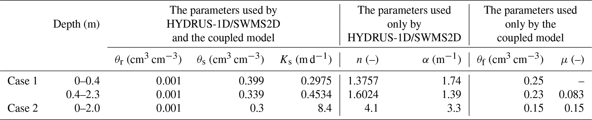
This case was to test the performance of the coupling scheme explained in Sect. 2.4. The case simulated a single field soil profile of the Hupselse Beek watershed in the Netherlands, which was used as a demo in the HYDRUS-1D technical manual (Šimůnek et al., 2008). The soil profile consists of a 0.4 m thick upper layer and a 1.9 m thick bottom layer. The depth of the root zone is 0.3 m. The hydraulic parameters of the two soil layers are presented in Table 1. The surface boundary condition involves actual precipitation and potential transpiration rate as shown in Fig. 3. The groundwater level was initially set at 0.55 m below the soil surface. Only one vertical soil column and one MODFLOW cell were used in the coupled model. The parameters used in the coupled model are also listed in Table 1. The results from HYDRUS-1D were used as the reference of this test case. The stress period ΔT was set as 5 d, and the MODFLOW time step Δt_s and the UBMOD time step Δt_u were both set to be 1 d. The spatial discretization was 0.1 m.

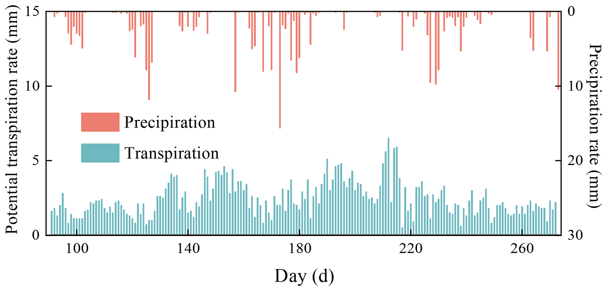
Figure 4 (a) The sketch of the 2-D recharge experiment of case 2. (b) The comparison of the water table between simulated results by the coupled model, SWMS2D, and observation data of case 2.

To figure out the influence of the temporal and spatial discretization as well as the stress period on the simulation results, scenarios with different temporal and spatial resolutions and the stress period of the coupled model were performed. Scenario 1 was set as the same as the above case. The UBMOD time steps of scenario 2 and scenario 3 were 0.5 and 2 d, while other inputs were the same as scenario 1. The spatial discretizations of scenario 4 and scenario 5 were set as 0.05 and 0.2 m, while other inputs were the same as scenario 1. The stress periods of scenario 6, scenario 7, and scenario 8 were set as 8, 10, and 15 d, while other inputs were the same as scenario 1. The eight scenarios were marked as S1–S8.

3.1.2 Case 2: two-dimensional (2-D) water table recharge experiment

This test case was used for model validation in a 2-D unsaturated–saturated flow system. The purpose of the case is to discuss the performance of the model under the condition with large lateral flux in the unsaturated zone. The numerical simulation of our model was compared with the data of a 2-D water table recharge experiment conducted by Vauclin et al. (1979). The experimental data have been used to test the variably saturated flow models (Clement et al., 1994) and coupled unsaturated–saturated flow models (Thoms et al., 2006; Twarakavi et al., 2008; Shen and Phanikumar, 2010; Xu et al., 2012). The 2-D domain is a rectangular sandy soil slab of $\mathrm{6.0}\times \mathrm{2.0}\times \mathrm{0.05}$ m. The initial pressure head is 0.65 m at the domain bottom. At the soil surface, a constant flux of q=3.55 m d⁻¹ is applied at the central 1.0 m, and the remaining soil surface is the no-flux boundary. Because of the symmetry of the flow system, only one-half of the domain (right side) with a size of 3.0 m × 2.0 m × 0.05 was simulated. The setup of the simulation is shown in Fig. 4a. No-flow boundaries were defined on the bottom and the left side, and the specified hydraulic head boundary of 0.65 m was set on the right side. The values of soil hydraulic parameters are listed in Table 1. The simulation period is 8 h. In our coupled model, there were 30 uniform rectangular cells used by MODFLOW, and there were 10 sub-areas defined to represent the unsaturated zone, which were numbered from left to right. The first and last sub-areas covered 0.2 and 0.4 m in the x direction, respectively, and each of the remaining sub-areas covered 0.3 m in the x direction. The first and second sub-areas were used to define the recharge boundary, while the other sub-areas were used to define the no-recharge boundary. The stress period ΔT was set as 1 h, and the initial MODFLOW time step Δt_s and UBMOD time steps Δt_u were set as 0.167 h. The spatial discretization of UBMOD was uniformly 0.1 m. The experiment was also simulated by using SWMS2D, which considered the lateral flow. The mean time step of SWMS2D was set to be 0.0225 h, and 20 200 finite elements were used.

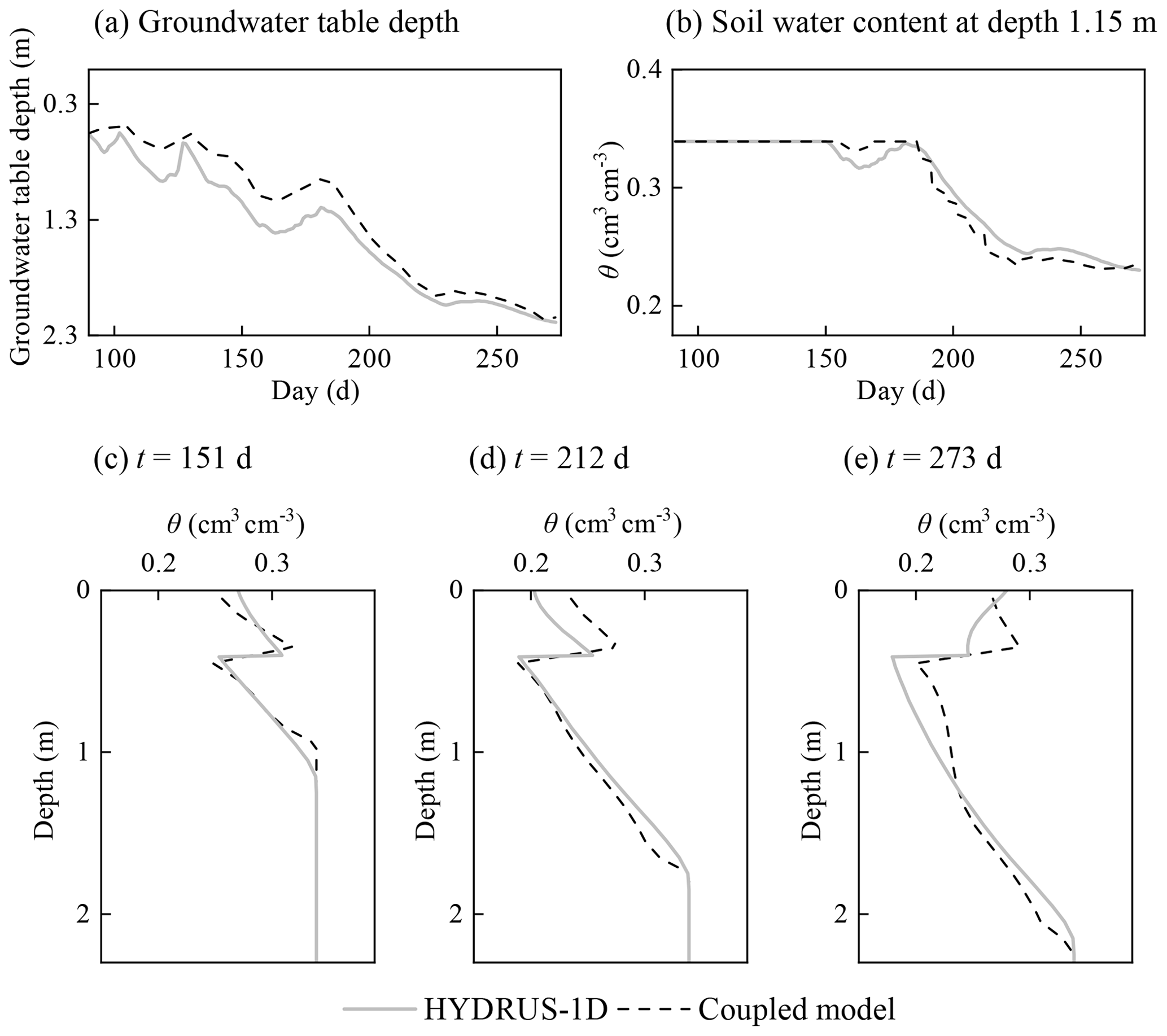
Figure 5 The comparison of the results calculated by HYDRUS-1D and the coupled model of case 1.

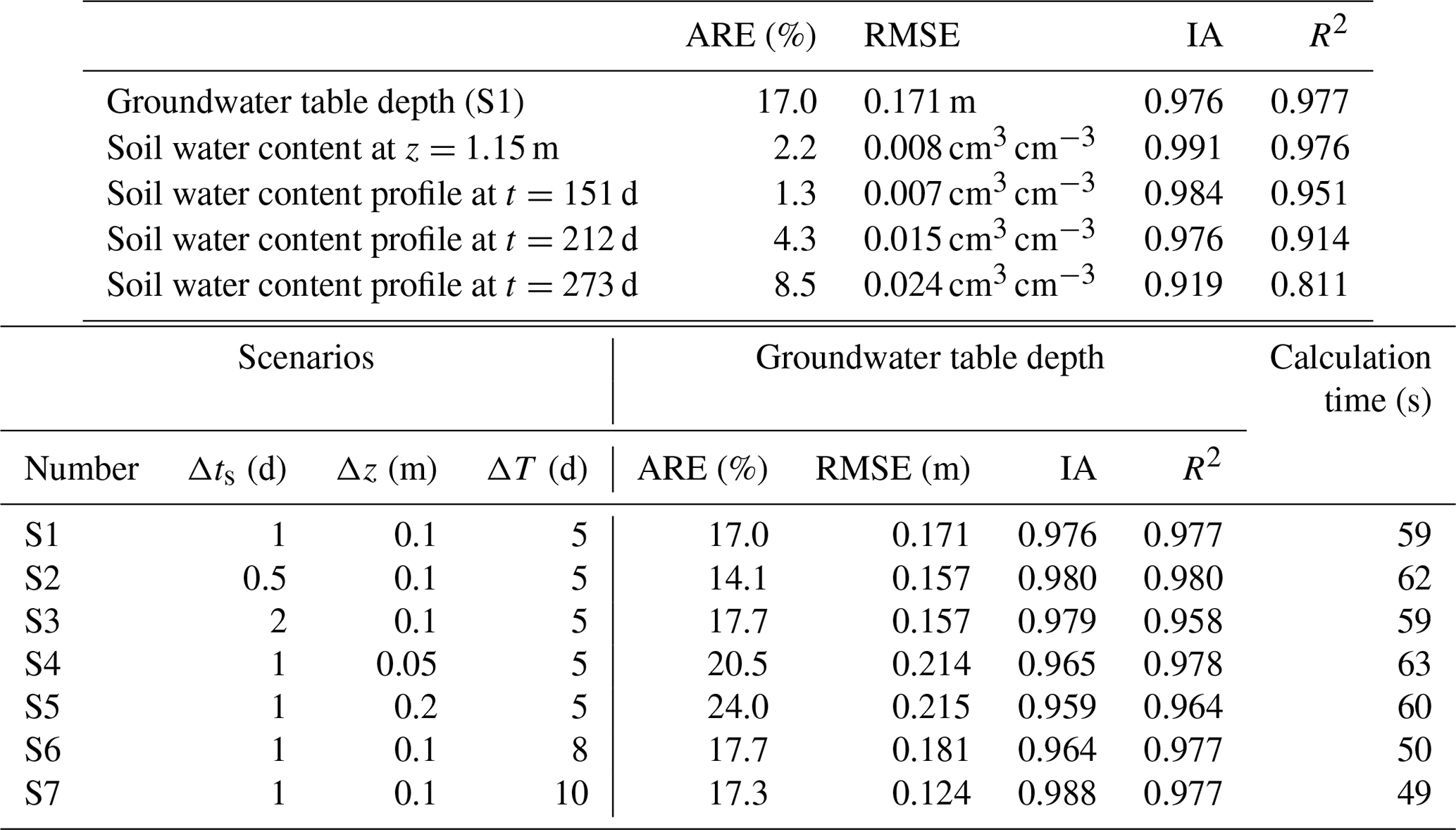
Table 2 The statistical index values of the coupled model of case 1.

3.2 Results and discussions of model performance

3.2.1 Computational accuracy of the coupling scheme

Figure 5 shows the comparison of the results simulated by HYDRUS-1D and the coupled model of case 1. The statistical indexes are listed in Table 2. Figure 5a demonstrates that the groundwater table depth calculated by the coupled model has a similar pattern to that of HYDRUS-1D. The ARE, RMSE, IA, and R² values were 17.0 %, 0.171 m, 0.976, and 0.977. The soil water contents at the depth of 1.15 m over time from the two models are compared in Fig. 5b. The ARE, RMSE, IA, and R² were 2.2 %, 0.008 cm³ cm⁻³, 0.991, and 0.976. The simulated soil water content profiles at different times are shown in Fig. 5c–e and the evaluation indexes demonstrate the satisfactory performance of the model. Moreover, the net groundwater consumption at the end of the simulation period was compared, which is 0.132 m calculated by the coupled model, and it is the same as that from HYDRUS-1D. In general, these results indicate that the coupled model can capture the flow information under the upward flux and the heterogeneous condition.

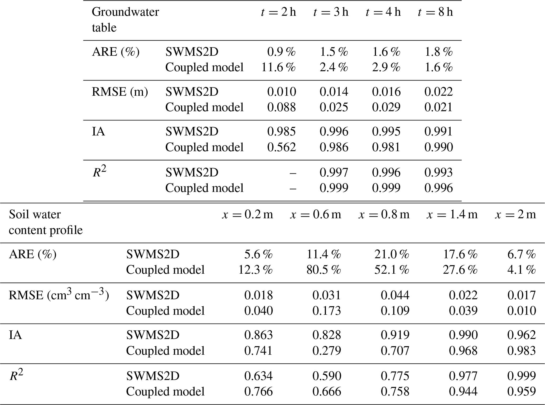
Table 3 The statistical index values of SWMS2D and the coupled model of case 2.

The deviations of groundwater table depth and soil water content from the coupled model and HYDRUS-1D can also be observed in Fig. 5. The deviations are caused by the different model structures of the coupled model and HYDRUS-1D. HYDRUS-1D solves the saturated–unsaturated flow together, and the groundwater table is determined at the depth with the matric potential equaling zero. The soil water content of the capillary fringe above the groundwater table is almost saturated. However, the UBMOD model cannot simulate the capillary fringe. And there is a parameter, the field capacity used to calculate the downward movement of soil water, which is defined under a free drainage condition. So, the coupled model could lead to the lower soil water content in the capillary fringe and higher groundwater table as shown in Fig. 5. And there is another parameter-specific yield used in the coupled model to determine the groundwater table, which is also attributed to the deviation of the groundwater table.

Figure 4b shows the comparison of simulated water tables at four different times using the coupled model and SWMS2D and the observation data in case 2. The index values are listed in Table 3. The coupled model matched the observation data well at the simulation times of 3, 4, and 8 h, with the ARE values smaller than 3 %, the RMSE values smaller than 0.03 m, and the IA and R² values close to 1. The observed and simulated soil water content profiles for the initial and ending times are presented in Fig. 6. The statistical index values are also listed in Table 3. The simulations by the coupled model agree well with the observations at the locations of x=0.2 m, x=1.4 m, and x=2 m (Fig. 6a, d, and e) where the lateral water flow is negligible. The calculated recharge is 3.55 m d⁻¹ per unit area when the flow becomes steady, which equals the input flux. These results demonstrate the accuracy of the coupled model and the reliability of the coupling scheme shown in Sect. 2.4.

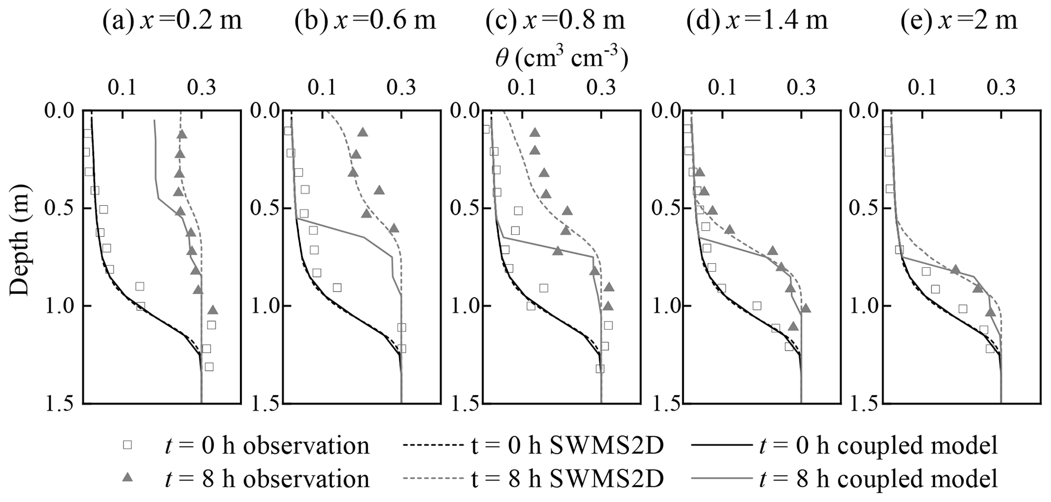
Figure 6 Comparison of soil water content profiles between the simulations from the coupled model, SWMS2D, and the observations at different locations: (a) x=0.2 m; (b) x=0.6 m; (c) x=0.8 m; (d) x=1.4 m; (e) x=2 m.

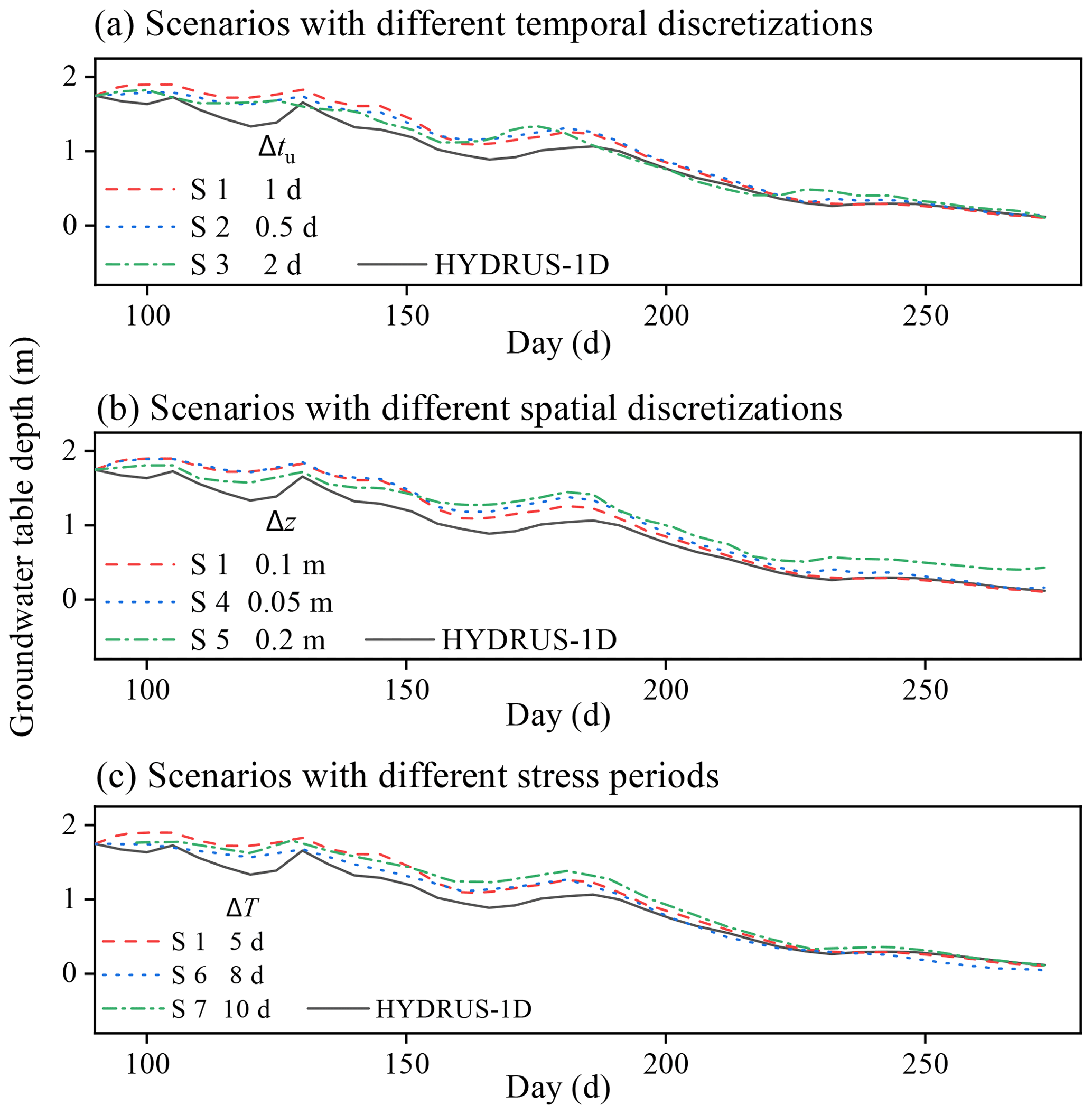
Figure 7 The influence of (a) temporal and (b) spatial discretization and (c) stress period on simulation results.

3.2.2 Influence of the temporal and spatial discretization as well as the stress period on simulation results

The groundwater table depths calculated by scenarios with different temporal discretizations (S1–S3) are compared with those from HYDRUS-1D in Fig. 7a. The statistical index values are shown in Table 2. It can be found that the water table depths calculated by different scenarios have the same variation trend. The ARE values of the three scenarios are smaller than 20 %, and the maximum RMSE value is 0.171 m. The IA and R² values are larger than 0.95. The groundwater table depths calculated by scenarios with different spatial discretizations (S1, S4, and S5) are compared with those from HYDRUS-1D in Fig. 7b. The ARE values of the three scenarios are smaller than 25 %. The maximum RMSE value is 0.215 m. The IA and R² values are larger than 0.95. The water table depths calculated by scenarios with different stress periods (S1, S6, S7, and S8) are compared with those from HYDRUS-1D in Fig. 7c. It should be noted that the model collapsed at the time of 227 d when the stress period is 15 d (S8). The statistical index values for S1, S6, and S7 are shown in Table 2. The ARE and RMSE values of the three scenarios are very similar. Considering the water balance method and empirical formulas adopted in the coupled model, the results calculated by all the scenarios except S8 are acceptable. These results indicate that the temporal and spatial discretizations have slight influence on the modeling results. It should be noted that the impact of the stress period on a certain scale (< 10 d in this case) has no significant impact on the simulation results. However, too large a stress period will cause improper results.

3.2.3 Limitations of the coupled model

Although the coupled model had a sufficient computational accuracy as shown above, there were limitations because of the quasi-3-D assumptions. The coupled model overestimates the water table at the time of 2 h in case 2 as shown in Fig. 4b. This is caused by a significant lateral flow in the unsaturated zone during the early period due to the relatively low initial soil water content condition. Therefore, a portion of the infiltration water in the first and second sub-areas should move in the lateral direction, instead of moving downward to the saturated zone as in the quasi-3-D model. The coupled model thus overestimates the recharge flux and results in a higher water table at the early period. Additionally, the simulated soil water content by the coupled model has poor performance at the locations of x=0.6 m and x=0.8 m (Fig. 6b and c). These two sub-areas are close to the recharge zone and affected by the lateral flow, which is ignored in the coupled model. These phenomena are similar to the results calculated by other quasi-3-D models (Xu et al., 2012; Shen and Phanikumar, 2010). Therefore, the coupled model overestimates the recharge and underestimates the soil water content when the lateral flow cannot be ignored. Its application should be limited to cases in which the soil flow mainly occurs in the vertical direction.

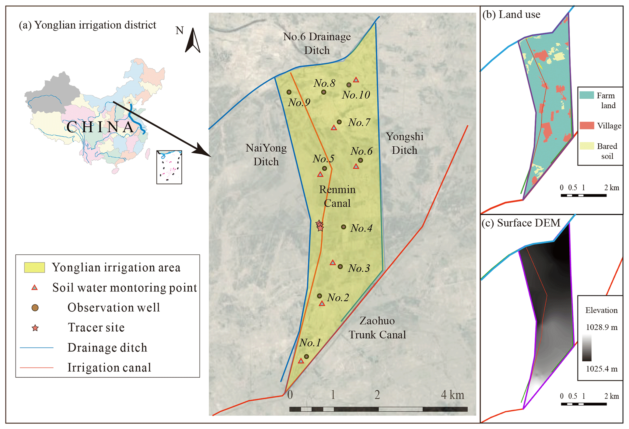
Figure 8 (a) The geographic location of the Yonglian irrigation area. (b) The land use map. (c) The surface DEM.

3.2.4 Water mass balance and computational cost

The mass balance error of the coupled model is small, with the maximum values 0.012 % in case 1 and 0.004 % in case 2, while they are 1.6 % for the HYDRUS-1D model and 0.133 % for the SWMS2D model. The cases were run on a 6 GB RAM, double 2.93 GHz intel Core (TM) 2 Duo CPU-based personal computer. The computational cost of different scenarios in case 1 of the coupled model ranges from 49 to 63 s as listed in Table 2. It is 1.4 s by HYDRUS-1D. The temporal and spatial discretization has slight influence on computational cost, while the stress period has significant influence on the computation cost. The iteration and information exchange are responsible for the high computational cost. For case 2, the computational costs of the coupled model and the SWMS2D model are 46 and 95 s, respectively. The coupled model has a better efficiency compared with the complete 2-D model due to its simpler numerical solutions and coarse discretization in space and time. The advantage of decreasing computational cost will be more obvious when the application scale becomes larger. Generally speaking, the coupled model provides satisfactory mass balance and good computational efficiency.

Figure 9 Daily climate data in the Yonglian irrigation area.

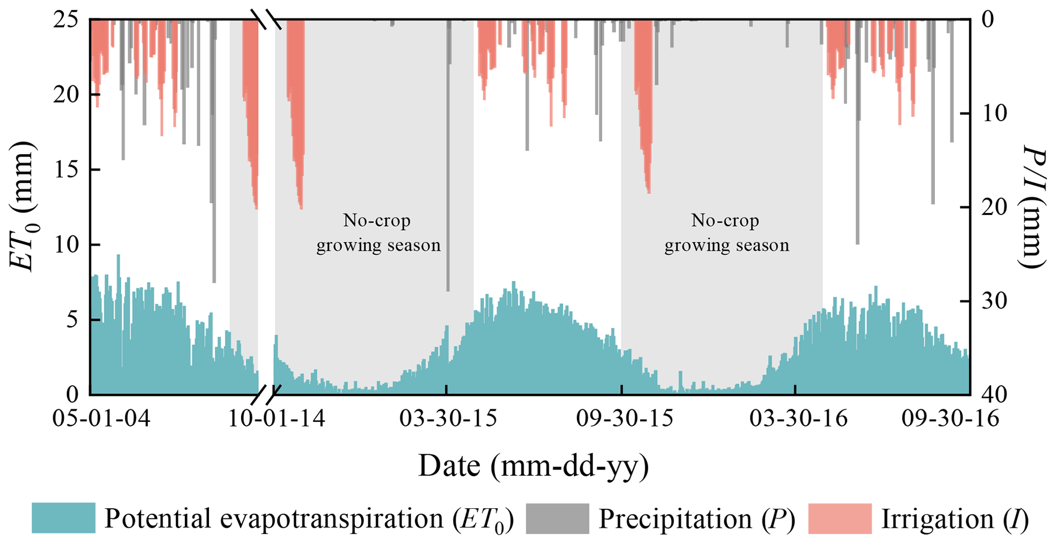
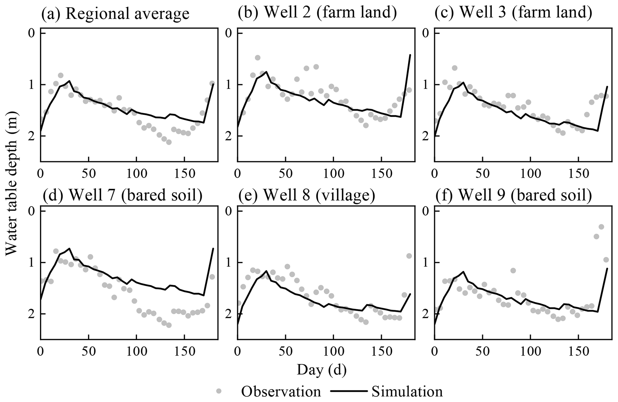
Figure 10 Comparison between simulated and observed water table depth of the real-world application.

4 Real-world application

4.1 Study site and input data

The coupled model was used to calculate the regional-scale groundwater recharge in a real-world case, where the shallow groundwater has significant impact on the soil water movement. Figure 8a shows the location of the study site, the Yonglian irrigation area (107^∘37^′19^′′–108^∘51^′04^′′ E, 40^∘45^′57^′′–41^∘17^′58^′′ N) in Inner Mongolia, China. The irrigation area is 12 km long from north to south and 3 km wide from east to west. The whole domain size is 29.75 km². The ground surface elevation decreases from 1028.9 to 1025.4 m from the southwest to the northeast. A 2-year tracer experiment from 2014 to 2016 was conducted to obtain the groundwater recharge (Yang, 2018), and the experimental locations are shown in Fig. 8a. This irrigation area has well-defined hydrogeological borders by the channel network. Since the Zaohuo Trunk Canal and No. 6 Drainage Ditch are filled with water over the simulation time, the first-kind boundary condition was applied to the two segments. The non-flow boundary condition was used for the other segments. The irrigation water of this area is diverted from the Renmin Canal. This irrigation area was divided into three sub-areas according to the land usage since they own significantly different upper boundary conditions, which are farm land, villages, and bared soil, as shown in Fig. 8b. The crop types in the farm land were not considered for determining the sub-areas. The surface digital elevation model (DEM) is shown in Fig. 8c.

The measured soil water content and groundwater table in the crop growing season from May to October of 2004 were used to calibrate the hydraulic parameters, and the tracer experiment from 2014 to 2016 was used for the groundwater recharge evaluation. A uniform daily rainfall rate was applied to the whole domain. The irrigation water was only applied to the farm land. Due to lack of the weather data in 2004, the potential evapotranspiration ET₀ was calculated by the measured evaporation data from the 20 cm pan (ET₂₀), multiplying by an empirical conversion coefficient. The empirical coefficient is 0.55, which was recommended by Hao (2016) by comparing monthly ET₀ and ET₂₀ with 8 years' data in this area. The ET₀ during 2014 to 2016 was calculated by using the Penman–Monteith equation. The precipitation, irrigation, and ET₀ are shown in Fig. 9. The crop growing season is from May to October, and the rest of the months are no-crop growing season. Based on the hydrogeological characteristics of the study area provided by the Geological Department of Inner Mongolia, the top aquifer within the depth of 7 m is loamy sand and loam with small hydraulic conductivity; an underlying sand aquifer with a thickness of 46 m has high permeability, and the sand aquifer lies on an impervious 1 m thick clay layer. The clay layer was used as the bottom of the simulation domain, and seven different geological layers were used in the MODFLOW model. The first layer was set to be the top aquifer, and the second aquifer was divided into six layers for numerical simulation. Ten groundwater monitoring wells were set in this district, and the groundwater tables were observed every 6 d. Well 1, well 2, well 3, well 5, and well 6 are located in farm land areas, well 4 and well 8 in villages, and well 7, well 9, and well 10 in bared soil areas. Additionally, there are five soil water content monitoring points in the farm land and two points in the bared soil area, as shown in Fig. 8a. Soil water contents within 1 m depth were observed one to three times every month from May to October in 2004.

Five GIS files are prepared as the shapefile files of the study domain, the land usage types, the boundary conditions, and raster files of the surface DEM and initial hydraulic head. There were 150 rows and 50 columns used in the MODFLOW model. The spatial discretization of UBMOD was set to be 0.1 m. The stress period ΔT was set as 5 d, and the MODFLOW time step Δt_s and UBMOD time step Δt_u were set as 1 d.

Table 4 The unsaturated hydraulic parameters of the real-world application.

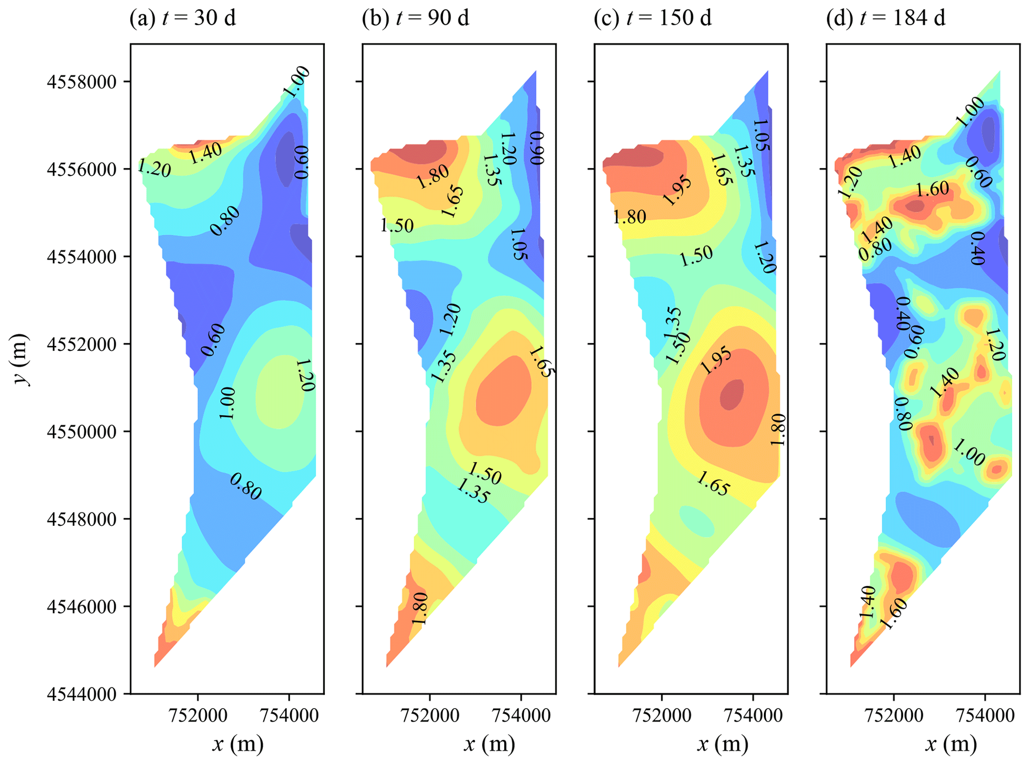
Figure 11 Spatial simulated water table depth at different output times of the real-world application.

4.2 Model calibration results

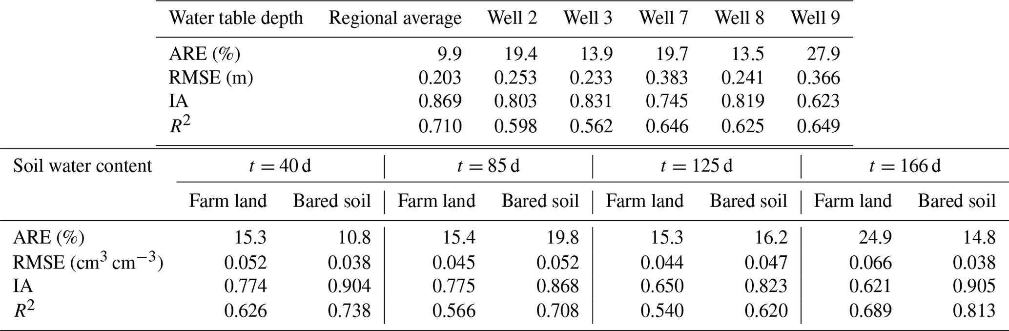
There are two soil types in the first layer as loamy sand and loam. The unsaturated hydraulic parameters of the two soils are listed in Table 4. The hydraulic conductivity of the top aquifer in MODFLOW was set as the same as the unsaturated layer, the hydraulic conductivity of the bottom sand aquifer was set as 3.5 m d⁻¹ during the calibration, and the specific yields of the top and bottom were set as 0.08 and 0.1, respectively. Figure 10 shows the comparison of the simulated and observed water table depths for the whole area and locations of different monitoring wells. The statistical index values are listed in Table 5. It can be found that the ARE, RMSE, IA, and R² values are 9.9 %, 0.203 m, 0.869, and 0.71 for the regional average water table depth. Larger deviations of simulated water table depth can be found for the locations of monitoring wells, with RMSE values ranging from 0.25 to 0.39 m. Figure 11 further shows the spatial distribution of the simulated water table depth at different output times. The increasing trend is obviously found in Fig. 11a to c in the crop growing season, during which the groundwater was consumed by crop transpiration and strong soil evaporation. When the intensive autumn irrigation happened after the 160th day, the water table depth in the farm land decreased rapidly, as shown in Fig. 11d. These results indicate that our model can reasonably simulate the water table depth trend in space and time.

Table 5 The statistical index values of the real-world application.

The recharge during the short term was calculated for further checking the results by comparing the results with those from reference papers. The calculated recharge in farm land during the autumn irrigation (from 16 to 31 October) is 93.3 mm, and the coefficient of recharge from the autumn irrigation is 0.37. Zhang (2011) suggested that the coefficient of recharge from the autumn irrigation is approximately 0.3. Yang (2016) proposed that the coefficient of the recharge from the autumn irrigation is between 0.36 and 0.4. Yu (2017) used the coefficient of recharge from autumn irrigation as 0.33 for the district. The calculated result is consistent with the previous studies. The phreatic evaporation coefficient was estimated during the period from 15 to 30 September with no precipitation or irrigation. The quantity of the recharge from saturated zone to unsaturated zone is 10.1 mm during the period in the farm land. The phreatic evaporation coefficient is 0.179, and the averaged water table depth is 1.51 m during the period. The phreatic evaporation coefficient measured by Wang (2002) is 0.172 at the depth of 1.5 m. The short-term results indicate the validity of the simulation results.

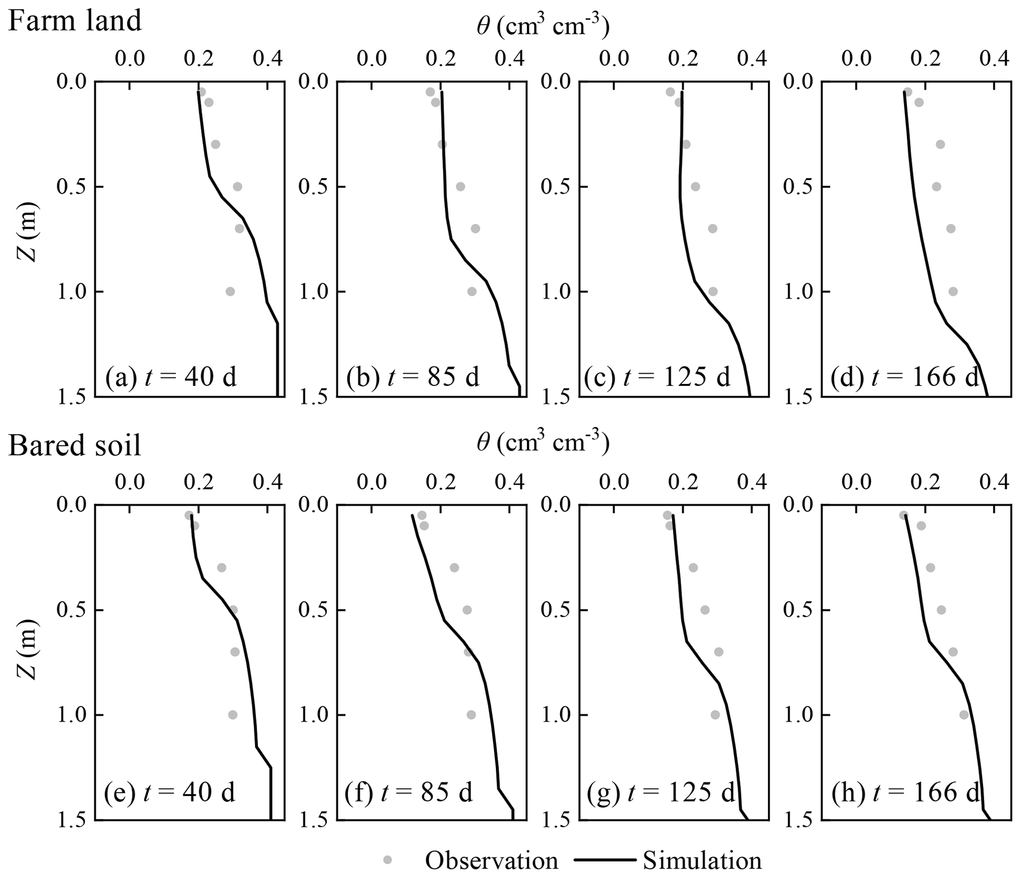
Figure 12 Comparison between simulated and observed regional average soil water content profiles of the real-world application.

Figure 12 shows the comparison between the simulated and average observed soil water content profiles of the farm land and bared soil at different times. The statistical index values are listed in Table 5. The ARE values of the farm land at the times of 40, 85, 125, and 166 d are 15.3 %–24.9 %, the RMSE values 0.044–0.066 cm³ cm⁻³, the IA values 0.621–0.775, and the R² values 0.54–0.689. The corresponding values for the bared soil are 10.8 %–19.8 %, 0.038–0.052 cm³ cm⁻³, 0.823–0.905, and 0.620–0.813, respectively. The larger measured soil water content in the root zone for the farm land can be observed than the simulations, while the simulated soil water content profiles in the bared soil agree well with the observations, as shown in Fig. 12. The reason may be that the sampling locations are at the border of fields, which leads to an overestimation of the soil water content in the root zone due to smaller crop root uptake.

Table 6 The recharge sources and results of the tracer experiment.

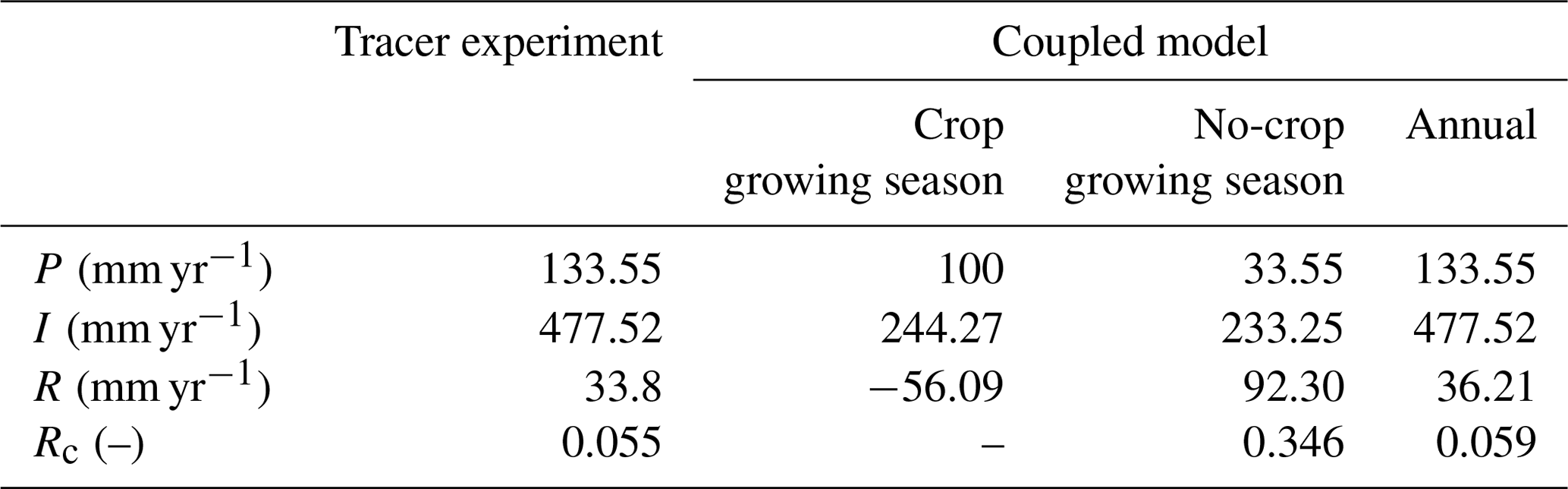
Note: P is the annual precipitation; I is the irrigation water; R is the annual recharge; and R_c is the recharge coefficient, $R_{\mathrm{c}}=R/(P+I)$.

Figure 13 The recharge rate in the farm land calculated by the coupled model.

The computational cost of the real-world application is 120 s, which is efficient considering the scale of the problem.

4.3 Regional groundwater recharge

In the tracer experiment, bromide (Br) was used as the tracer for calculating groundwater recharge. The tracer was injected at 1 m depth at two locations shown in Fig. 8a in October 2014. Based on two sampling locations in October 2015 and 2016, the downward recharge is estimated according to the movement distance of the tracer peak and the average water content from the initial position of the tracer to the final position (Tan et al., 2014). The soil water content at the depth of 1 m is relatively stable according to the measurements and the results of Peng (2015), which ensures the reliability of the experiment. As shown in Table 6, the annual average recharge R is 33.8 mm yr⁻¹, and the recharge coefficient is 0.055 during the period of 2014–2016.

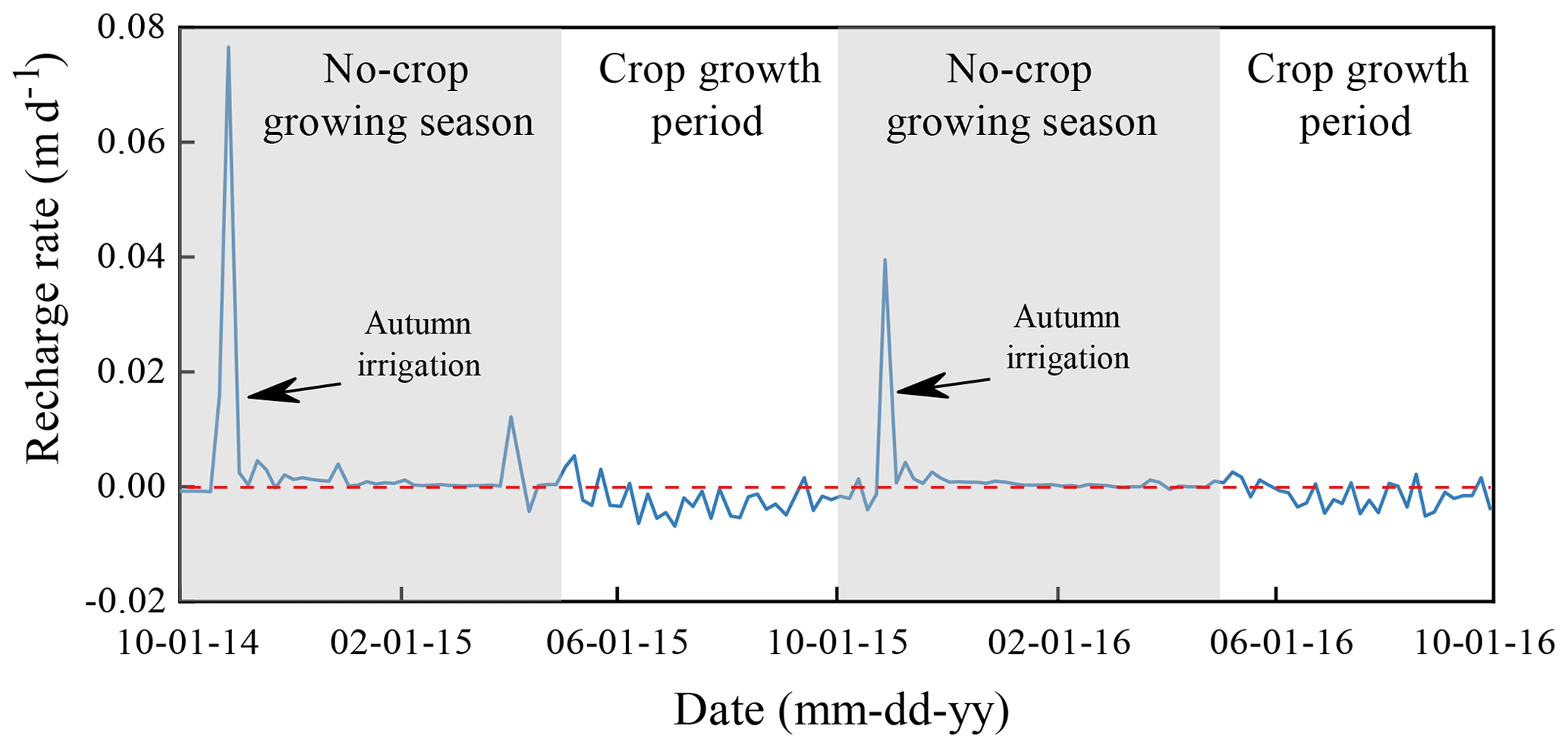
The calibrated coupled model was used to estimate the groundwater recharge from 1 October 2014 to 30 September 2016. Figure 13 shows the time series of simulated recharge rate in the farm land, and Table 6 lists the simulation results. The simulation results indicate that groundwater is recharged in the no-crop growing season and consumed in the crop growing season. The two peak values of groundwater recharge in Fig. 13 are due to the autumn irrigation after harvest for washing salt out. The no-crop growing season provides 92.30 mm yr⁻¹ groundwater recharge over a year and the average recharge coefficient is 0.346, which indicates that the autumn irrigation in the no-crop growing season provides the primary groundwater recharge in the year. In the crop growth season, the recharge is negative, which means that groundwater is consumed by crop transpiration and soil evaporation. As calculated by the coupled model, the annual groundwater recharge is 36.21 mm yr⁻¹ during the period from 1 October 2014 to 30 September 2016 in the farm land, which is similar to the result of the tracer experiment. The results confirm the coupled model for groundwater recharge evaluation, which is helpful for scheduling the irrigation amount in the crop growing season under the water saving policies.

5 Conclusions

This study developed a new quasi-3-D coupled model for the purpose of practical modeling of unsaturated–saturated flow at the regional scale. The UBMOD 1-D water balance model describing the unsaturated soil water flow was integrated with MODFLOW iteratively. A developed framework implemented the modeling procedures and provided the pre- and post-processing tools. The model was evaluated by using both synthetic numerical examples and real-world experimental data. The major conclusions drawn from this research are as follows.

1. The new iteration coupling scheme iteratively integrating a hydrodynamic model with a water balance model is reliable. The vertical net recharge and the depth of the unsaturated zone are effective to be used as the exchange information to couple the unsaturated zone and saturated zone.

2. The satisfactory results in the two testing examples demonstrate the effectiveness of the new quasi-3-D model with an acceptable calculative efficiency and well-maintained saturated zone and unsaturated zone mass balance.

3. The spatial and temporal discretization has slight impact on the simulation results. The stress period should be not too large and it also has slight impact on the simulation results in a certain range.

4. The model gives a satisfactory performance for calculating the groundwater recharge measured from the tracer experiment. The calculated annual groundwater recharge is 36.21 mm yr⁻¹ and the recharge coefficient is 0.059 in the study area.

5. The coupled model should not be used for problems with substantial lateral flow in the unsaturated zone because of the quasi-3-D assumptions used in the model.

6. The coupled model could lead to a higher groundwater table depth since it ignores the capillary fringe.

Appendix A

UBMOD is a water balance model based on a hybrid of numerical and statistical methods. Compared with the traditional ones, the model can simulate upward soil water movement in heterogeneous situations.

There are four major components to describe the soil water movement in the UBMOD model, as shown in Fig. A1. Firstly, the vertical soil column is divided into a cascade of “buckets” and each “bucket” corresponds to a soil layer. The “buckets” will be filled to saturation from the top layer to the bottom layer if there is infiltration, which is referred to as the allocation of infiltration water. Specifically speaking, the infiltration water first fills the top “bucket”, then the excessive infiltration water moves downward to the next “bucket”, until all the infiltration water is allocated in the “buckets”, as shown in Fig. A1a. The governing equation of layer i is

$$\begin{array}{}\text{(A1)}& q_i=min\left(M_i\times \left({\mathit{\theta }}_{\mathrm{s},i}-{\mathit{\theta }}_i\right),I-I_{\mathrm{d},i-\mathrm{1}}\right),\end{array}$$

where i indicates the vertical soil layer, i=1, …, j; q_i is the amount of allocated water per unit area of layer i (L); M_i is the thickness of layer i (L); θ_i is the initial soil water content of layer i (L³ L⁻³); θ_s,i is the saturated soil water content of layer i (L³ L⁻³); I is the quantity of infiltration water per unit area (L); $I_{\mathrm{d},i-\mathrm{1}}$ is the consumed infiltration water per unit area by upper layers for the specific layer i (L); and $I-I_{\mathrm{d},i-\mathrm{1}}$ is the infiltration water applied to the upper boundary of soil layer i (L). The infiltration rate I is input data in the model, and the partitioning of rainfall between infiltration and runoff has not been considered by now. As shown in Fig. A1a, the first three layers are filled to saturation, and the fourth layer is filled with the residual infiltration water.

Secondly, when the soil water content exceeds the field capacity, the soil water will move downward driven by the gravitational potential. The governing equation is

$$\begin{array}{}\text{(A2)}& {\displaystyle \frac{\partial \mathit{\theta }}{\partial t}}=-{\displaystyle \frac{\partial K\left(\mathit{\theta }\right)}{\partial z}},\end{array}$$

where t is the time (T); K(θ) is the unsaturated hydraulic conductivity (L T⁻¹) as a function of soil water content; z is the elevation in the vertical direction (L). The vertical coordinate is positive downward. The unsaturated hydraulic conductivity K(θ) in Eq. (A2) is a function of soil water content θ. The relationship between K(θ) and θ is characterized by empirical formulas for the purpose of simplifying calculation and eliminating the soil hydraulic parameters. These empirical formulas are referred to as drainage functions. The commonly used equations are listed in Table A1.

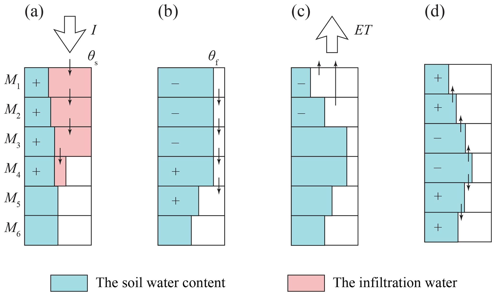
Figure A1 The schematic procedures of UBMOD with (a) the allocation of the infiltration water, (b) the soil water advective movement driven by the gravitational potential, (c) the source/sink terms, and (d) the soil water diffusive movement driven by the matric potential.

Thirdly, the source/sink terms are used to account for soil evaporation and crop transpiration. The governing equation is as follows:

$$\begin{array}{}\text{(A3)}& {\displaystyle \frac{\partial \mathit{\theta }}{\partial t}}=-W,\end{array}$$

where W is the source/sink term (T⁻¹). The Penman–Monteith formula and Beer's law (also known as a Ritchie-type equation) are adopted in UBMOD to estimate the potential soil evaporation E_p and potential crop transpiration T_p. Then E_p and T_p are distributed to each layer based on the evaporation cumulative distribution function and the root density function. The actual soil evaporation and crop transpiration are obtained by discounting E_p and T_p with the soil water stress coefficient.

Lastly, we calculate the diffusive movement driven by the matric potential. The governing equation is

$$\begin{array}{}\text{(A4)}& {\displaystyle \frac{\partial \mathit{\theta }}{\partial t}}={\displaystyle \frac{\partial }{\partial z}}\left(D\left(\mathit{\theta }\right){\displaystyle \frac{\partial \mathit{\theta }}{\partial z}}\right),\end{array}$$

where D(θ) is the hydraulic diffusivity (L² T⁻¹), and $D\left(\mathit{\theta }\right)=K\left(\mathit{\theta }\right)\times \partial h/\partial \mathit{\theta }$, where h is the matric potential (L). The finite-difference method is used to solve the governing equation. A new empirical formula is presented to describe the hydraulic diffusivity D(θ). The expression formula of D(θ) has an exponential form as

$$\begin{array}{}\text{(A5)}& D\left(\mathit{\theta }\right)={\mathrm{10}}^{a\times S\left(\mathit{\theta }\right)+b},\end{array}$$

where S(θ) is the effective saturation (–); a and b are two intermediate parameters. In order to eliminate the parameters, we calculate the hydraulic diffusivity D(θ) of different soils by the van Genuchten model firstly, and then fit the hydraulic diffusivity D(θ) by Eq. (A5). Furthermore, we establish the relationship between the two intermediate parameters (a and b) and the saturated hydraulic conductivity K_s as

$$\begin{array}{}\text{(A6)}& \left\{\begin{array}{l}b=-\mathrm{3.55}+\mathrm{0.55}\times {\log }_{\mathrm{10}}\left(K_{\mathrm{s}}\right)-\mathrm{1.36}\times {\log }_{\mathrm{10}}{\left(K_{\mathrm{s}}\right)}^{\mathrm{2}}\\ a=\mathrm{3.72}+\mathrm{0.61}\times {\log }_{\mathrm{10}}\left(K_{\mathrm{s}}\right)+\mathrm{1.52}\times {\log }_{\mathrm{10}}{\left(K_{\mathrm{s}}\right)}^{\mathrm{2}}\end{array}\right.\end{array}$$

By following the steps above, the hydraulic diffusivity D(θ) of a specific soil type can be estimated with three physical meaning parameters (K_s, θ_s, and θ_r).

Table A1 Empirical drainage functions representing the relationship between the unsaturated hydraulic conductivity K(θ) and soil water content θ.

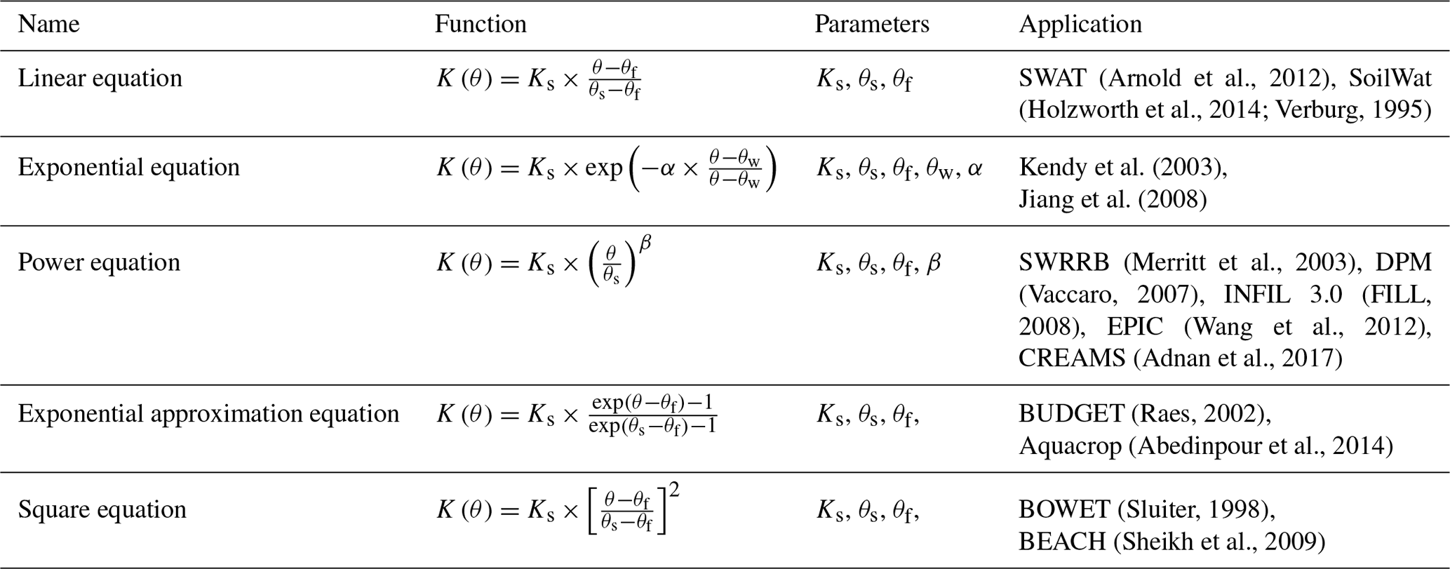
Note: the parameters K_s, θ_s, and θ_f are the saturated hydraulic conductivity (L T⁻¹), the saturated water content (L³ L⁻³), and the field capacity (L³ L⁻³); θ_w is the soil water content at wilting point (L³ L⁻³); α in the exponential equation is a site-specific parameter determined mainly from soil characteristics, and it has an inverse relationship with K_s, and the value ranges between 10 and 30 (Jiang et al., 2008). The parameter β in the power equation ensures K(θ) approaches zero when θ approaches θ_f, and Arnold et al. (1990) proposed an empirical formula as $\mathit{\beta }=-\mathrm{2.655}/\log \left({\mathit{\theta }}_{\mathrm{f}}/{\mathit{\theta }}_{\mathrm{s}}\right)$.

Soil water content is discontinuous at the material interface when a soil profile is heterogeneous. When adopting the van Genuchten model to represent the soil water characteristics, Eq. (A4) can be expressed as

$$\begin{array}{}\text{(A7)}& \begin{array}{rl}& {\displaystyle \frac{\partial \mathit{\theta }}{\partial t}}={\displaystyle \frac{\partial }{\partial z}}\\ & \left(D\left(\mathit{\theta }\right)\left({\displaystyle \frac{\partial \mathit{\theta }}{\partial z}}-\left({\displaystyle \frac{\partial \mathit{\theta }}{\partial {\mathit{\theta }}_{\mathrm{s}}}}{\displaystyle \frac{\partial {\mathit{\theta }}_{\mathrm{s}}}{\partial z}}+{\displaystyle \frac{\partial \mathit{\theta }}{\partial {\mathit{\theta }}_{\mathrm{r}}}}{\displaystyle \frac{\partial {\mathit{\theta }}_{\mathrm{r}}}{\partial z}}+{\displaystyle \frac{\partial \mathit{\theta }}{\partial \mathit{\alpha }}}{\displaystyle \frac{\partial \mathit{\alpha }}{\partial z}}+{\displaystyle \frac{\partial \mathit{\theta }}{\partial n}}{\displaystyle \frac{\partial n}{\partial z}}\right)\right)\right),\end{array}\end{array}$$

where α and n are two parameters in the van Genuchten model. The two terms $\partial \mathit{\theta }/\partial {\mathit{\theta }}_{\mathrm{s}}$ and $\partial \mathit{\theta }/\partial {\mathit{\theta }}_{\mathrm{r}}$ can be easily calculated. The value of $\partial \mathit{\theta }/\partial \mathit{\alpha }$ is close to zero, which can be ignored. A regression formula is developed to characterize the relationship between n and the saturated hydraulic conductivity K_s. The specific equations are shown as follows:

$$\begin{array}{}\text{(A8)}& \left\{\begin{array}{l}{\displaystyle \frac{\partial \mathit{\theta }}{\partial {\mathit{\theta }}_{\mathrm{s}}}}=S\left(\mathit{\theta }\right),\\ {\displaystyle \frac{\partial \mathit{\theta }}{\partial {\mathit{\theta }}_{\mathrm{r}}}}=\mathrm{1}-S\left(\mathit{\theta }\right),\\ {\displaystyle \frac{\partial \mathit{\theta }}{\partial n}}=\left({\mathit{\theta }}_{\mathrm{s}}-{\mathit{\theta }}_{\mathrm{r}}\right)S\left(\mathit{\theta }\right)\\ \left[{\displaystyle \frac{\ln \left(S\left(\mathit{\theta }\right)\right)}{n\left(n-\mathrm{1}\right)}}-{\displaystyle \frac{n-\mathrm{1}}{n^{\mathrm{2}}}}\left(S{\left(\mathit{\theta }\right)}^{n/\mathrm{1}-n}-\mathrm{1}\right)\right.\\ \left.\ln \left(S{\left(\mathit{\theta }\right)}^{n/\mathrm{1}-n}-\mathrm{1}\right)S{\left(\mathit{\theta }\right)}^{-n/\mathrm{1}-n}\right],\\ n=\mathrm{0.9505}+\mathrm{0.8883}{e}^{\mathrm{0.7751}\times {\log }_{\mathrm{10}}\left(K_{\mathrm{s}}\right)}.\end{array}\right.\end{array}$$

Therefore, the diffusive term of the heterogeneous soil can be calculated. With the help of the diffusive term, UBMOD can consider upward soil water movement, which is ignored by most water balance models.