the Creative Commons Attribution 4.0 License.
the Creative Commons Attribution 4.0 License.
 | 09 Apr 2019
Identifying El Niño–Southern Oscillation influences on rainfall with classification models: implications for water resource management of Sri Lanka
Thushara De Silva M.
George M. Hornberger
Seasonal to annual forecasts of precipitation patterns are very important for water infrastructure management. In particular, such forecasts can be used to inform decisions about the operation of multipurpose reservoir systems in the face of changing climate conditions. Success in making useful forecasts is often achieved by considering climate teleconnections such as the El Niño–Southern Oscillation (ENSO) and Indian Ocean Dipole (IOD) as related to sea surface temperature variations. We present a statistical analysis to explore the utility of using rainfall relationships in Sri Lanka with ENSO and IOD to predict rainfall to the Mahaweli and Kelani River basins of the country.
Forecasting of rainfall as the classes flood, drought, and normal is helpful for water resource management decision-making. Results of these models give better accuracy than a prediction of absolute values. Quadratic discrimination analysis (QDA) and classification tree models are used to identify the patterns of rainfall classes with respect to ENSO and IOD indices. Ensemble modeling tool Random Forest is also used to predict the rainfall classes as drought and not drought with higher skill. These models can be used to forecast the areal rainfall using predicted climate indices. Results from these models are not very accurate; however, the patterns recognized provide useful input to water resource managers as they plan for adaptation of agriculture and energy sectors in response to climate variability.
- Article
(5612 KB) - Full-text XML
- BibTeX
- EndNote


The spatial and temporal uncertainty of water availability is one of the major challenges in water resource management. Understanding patterns and identifying trends in seasonal to annual precipitation are very important for water infrastructure management. In particular, forecasts that incorporate such information can be used to inform decisions about the operation of multipurpose reservoir systems in the face of changing climate conditions.
Success in making useful forecasts is often achieved by considering climate teleconnections such as the El Niño–Southern Oscillation (ENSO) as related to sea surface temperature variations and air pressure over the globe using empirical data (Amarasekera et al., 1997; Denise et al., 2017; Korecha and Sorteberg, 2013; Seibert et al., 2017). Also, modes of variability of other tropical oceans can be related to regional precipitation (Dettinger and Diaz, 2000; Eden et al., 2015; Maity and Nagesh Kumar, 2006; Malmgren et al., 2007; Ranatunge et al., 2003; Suppiah, 1996; Roplewski and Halpert, 1996). For example, the effect of the Indian Ocean Dipole (IOD) is identified as independent of the ENSO effect (Eden et al., 2015). Pacific decadal oscillation (PDO), Atlantic multi-decadal mode oscillation (AMO), ENSO, and IOD teleconnections to precipitation have been found by many studies over the globe. Variations in precipitation in the United States are explained by ENSO, PDO, and AMO (Eden et al., 2015; National Oceanic and Atmospheric Administration, 2017; Ward et al., 2014); in African countries by ENSO, AMO, and IOD (Reason et al., 2006); and in southeastern Asian countries by ENSO: Indonesia (Lee, 2015; Nur'utami and Hidayat, 2016), Thailand (Singhrattna et al., 2005b), China (Cao et al., 2017; Ouyang et al., 2014; Qiu et al., 2014), Australia (Bureau of Meteorology, 2012; Verdon and Franks, 2005), and central and south Asia (Gerlitz et al., 2016).
The impact of ENSO and IOD on the position of the intertropical convergence zone (ITCZ) has been identified as a primary factor driving south Asian tropical climate variations. South Asian countries get precipitation from two monsoons from the movements of ITCZ in boreal summer (2∘ N) and boreal winter (8∘ S). The southwestern monsoon (summer monsoon) is during June–August and the northeastern monsoon (winter monsoon) is during December–February (Schneider et al., 2014). Climate teleconnections have been studied for summer monsoons (Singhrattna et al., 2005a; Surendran et al., 2015) and winter monsoons (Zubair and Ropelewski, 2006). A negative correlation of ENSO with the Indian summer monsoon has been identified (Jha et al., 2016; Surendran et al., 2015).
The objective of this study is to explore the climate teleconnection to dual monsoons and inter-monsoons. Water resource management decisions are typically based on precipitation throughout the year, and it is extremely important to explore the possibility that rainfall might be related to teleconnection indices for which seasonal forecasts are available. Sri Lanka is a south Asian country that gets rainfall from two monsoons and two inter-monsoons. We explore ENSO and IOD climate teleconnection to Sri Lanka precipitation throughout the year. Past studies have identified a climate teleconnection linking precipitation to climate indices for several months and monsoon seasons, and shown the importance of these for forecasting rainfall in river basins (Chandimala and Zubair, 2007; Chandrasekara et al., 2017). We extend these analyses across monsoon and inter-monsoon seasons.
Although rainfall anomalies may be correlated strongly with teleconnection indices, the scatter in the data can be large, making predictions from regression models have high uncertainty. However, water managers may act on information about whether rainfall is expected to be abnormally low or high. Seasonal precipitation is generally forecasted in broad categories. For example, the US National Weather Service forecasts seasonal precipitation as above normal, below normal, and normal (National Oceanic and Atmospheric Administration, 2018). The International Research Institute for Climate and Society also forecasts seasonal precipitation as above, below, and near normal (International Research Institute for Climate Society, 2018). We chose to follow a similar approach and investigate river basin rainfall teleconnections to climate indices with classification models. If reasonably accurate relationships can be developed, they will be useful for water resource management. For example, in Sri Lanka decisions about allocations of water for irrigation and hydropower could be improved with estimates of when low rainfall seasons are likely.
Sri Lanka is an island in the Indian Ocean (latitude 5∘55′–9∘50′ N, longitude 79∘40′–81∘53′ E). Mean annual rainfall varies from 880 to 5500 mm across the island. The rainfall distribution is determined by the monsoon system of the Indian Ocean interacting with the elevated land mass in the interior of the country. The country is divided into three climatic zones according to the rainfall distribution: humid zone (wet zone) (annual rainfall > 2500 mm), intermediate zone (2500 mm < rainfall < 1750 mm), and arid zone (dry zone) (rainfall < 1750 mm) (Department of Agriculture Sri Lanka, 2017).
Sri Lanka, a water-rich country, has 103 river basins varying from 9 to 10 448 km2. A large fraction of the water resource management infrastructure of the country is associated with the Mahaweli and Kelani River basins. The catchment areas of the Mahaweli and Kelani are 10 448 and 2292 km2, respectively. The two rivers start from the central highlands. Mahaweli, the longest river, travels to the ocean 331 km in the eastern direction and the Kelani 145 km in the western direction. Average annual discharge volume for the Mahaweli and Kelani basins is 26 368×106 and 8660×106 m3 respectively (Manchanayake and Madduma Bandara, 1999). The Kelani River basin is totally inside the humid zone, whereas the Mahaweli River basin migrates through all three climate zones (Fig. 1).

The temporal pattern of rainfall in Sri Lanka can be divided into four seasons as follows.
-
Generally there is low precipitation across the country from the northeastern monsoon (NEM), which includes most precipitation during January to February. The arid zone of the country receives significant precipitation from the NEM, while the humid zone receives very little rainfall during this period.
-
The whole country receives precipitation from the first inter-monsoon (FIM) during March to April. However, rainfall during this period is not very high across the country.
-
The highest precipitation for the country is from the southwestern monsoon (SWM) during May to September. However, only the humid zone receives high precipitation during this season.
-
The whole country receives precipitation from the second inter-monsoon (SIM) during October to December. Generally, precipitation from SIM is higher than FIM.
The time periods of the NEM and SIM are generally considered to be December to February and October to November, respectively (Department of Meteorology Sri Lanka, 2017; Malmgren et al., 2003; Ranatunge et al., 2003). However, considering the bulk amount of water received from the monsoon, we consider January and February as the period of NEM and October to December as the period of SIM.
Reflecting the rainfall seasons, the country has two agriculture seasons: “Yala” (April–September) and “Maha” (October–March). Because the arid zone receives minimal precipitation during the SWM, the agricultural systems (165 000 ha) developed under the Mahaweli multipurpose project depend on irrigation water during the Yala season. The country depends on stored water to drive hydropower year round. The Mahaweli and Kelani hydropower plants of 810 and 335 MW capacity serve as peaking and contingency reserve power to the power system (Ceylon Electricity Board, 2015). Management of reservoir systems is performed to cater to both irrigation and hydropower requirements.
2.1 Subbasin rainfall (areal rainfall)
Monthly rainfall data for the years 1950–2013 are used for the study (Ceylon Electricity Board, 2017). River basin rainfall was calculated using the Thiessen polygon method (Viessman, 2002). The Mahaweli River basin is divided into 16 Thiessen polygons and the Kelani River basin is divided into 11 Thiessen polygons (Fig. 1). Since this study does not aim to explore rainfall across subbasins, we do not use digital elevation maps to define the subbasins. Considering the importance of subbasins for the reservoir catchment and for water use, eight subbasins are selected for analysis. Morape, Randenigala, Peradeniya, Manampitiya, and Bowatenna represent the major Mahaweli reservoir catchments and irrigation tanks, and Norton Bridge, Norwood, and Laxapana represent the Kelani basin reservoir catchments. The catchment of the major Mahaweli River reservoir cascade (Kotmale, Victoria, Randenigala, Rantambe, Bowatenna) is represented by Morape and Peradeniya located in the humid zone and by Randenigala and Bowatenna located in the intermediate zone. The major arid zone irrigation catchments of the Mahaweli are represented by Manampitiya. The catchment of the Kelaniya reservoir cascade (Norton Bridge and Moussakele) in the humid zone is represented by Laxapana, Norton Bridge, and Norwood.
We calculate the rainfall for the four seasons, NEM, FIM, SWM, and SIM for 64 years of historical data. Rainfall anomalies are calculated by reducing the seasonal mean rainfall (Eq. 1) and standardized anomalies are calculated by dividing the rainfall anomalies by the standard deviation (SD) (Eq. 2).
Here is the average of seasonal rainfall, XANM is the rainfall anomaly, and XS_ANM is the standardized rainfall anomaly.
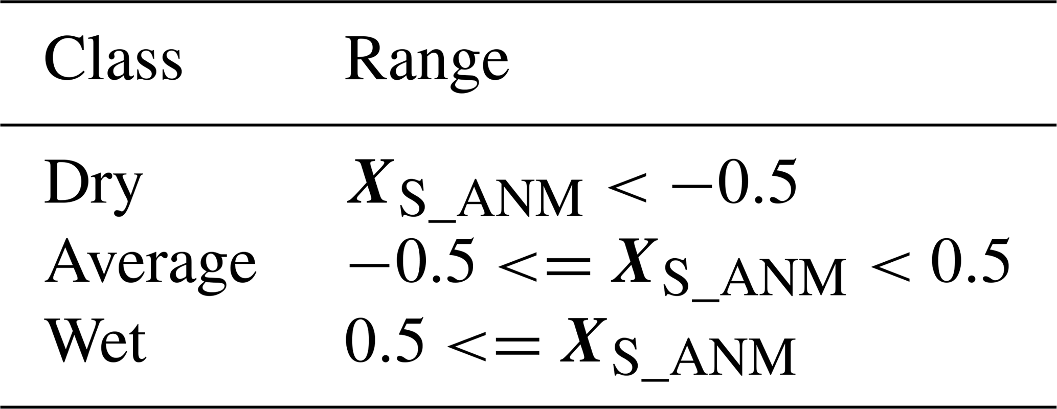
Standardized rainfall anomalies are divided into three classes as dry, average, and wet (Table 1). A normality test for the rainfall data classes is performed using the Shapiro–Wilk test. If the rainfall data are not normally distributed, log (e), square root or square functions are used to transform the data into normally distributed data sets (Fig. A1). Extreme seasonal precipitation has been defined statistically in different ways using statistical thresholds (Easterling et al., 2000; Jentsch et al., 2007; Smith, 2011). We use 0.5 as a threshold to define three classes, which results in fairly evenly distributed data across the three classes (Fig. A2).
2.2 ENSO and IOD indices
The ENSO phenomenon is represented by the multivariate ENSO index (MEI) and NINO34, NINO3, and NINO4 indices, and the Indian Ocean Dipole phenomenon is represented by the dipole mode index (DMI) index. The NINO34, NINO3, and NINO4 indices are based on tropical sea surface temperature anomalies (National Center for Atmospheric Research, 2018), and the multivariate ENSO index (MEI) is based on sea-level pressure, zonal and meridional components of the surface wind, sea surface temperature, surface air temperature, and total cloudiness fraction of the sky (National Oceanic and Atmospheric Administration, 2017). The Indian Ocean Dipole (IOD) is an oscillation of sea surface temperature in the equatorial Indian Ocean between the Arabian Sea and south of Indonesia (Bureau of Meteorology, 2017). The IOD is identified as relevant to the climate of Australia (Power et al., 1999) and countries surrounded by the Indian Ocean in southern Asia (Chaudhari et al., 2013; Maity and Nagesh Kumar, 2006; Qiu et al., 2014; Surendran et al., 2015). The dipole mode index (DMI) is used to represent the IOD capturing the west and eastern equatorial sea surface temperature gradient.
Data used for the analyses are NINO34, NINO3, NINO4, and MEI monthly data from the years 1950–2013 (National Oceanic and Atmospheric Administration, 2017; National Center for Atmospheric Research, 2018) and the DMI monthly data from 1950 to 2013 (HadISST data set, Japan Agency for Marine Earth Science and Technology, 2019). Because we analyzed the data in rainfall seasons, values of the climate indices over the season are averaged. For example for the NEM season, the MEI value is the average of January and February monthly values and for the SWM season, DMI is the average of May, June, July, and September values.
Seasonal values of MEI and DMI were used as the predictors to classify seasons into the three rainfall classes. The total data set is divided into 75 % for training the model and 25 % for testing model performance. Quadratic discriminant analysis (QDA) and classification trees were selected for the analyses. A random forest model also was applied to investigate the reliability of a cross-validated statistical forecast tool based on an advance estimate of MEI and DMI. We used the R programming language to carry out the statistical analyses. R packages caret, tree, randomForest, fitdistriplus, devtools, and quantreg are used for the studies.
3.1 Quadratic discriminant analysis (QDA)
The mathematical formulation of QDA can be derived from the Bayes theorem assuming that observations from each class are drawn from a Gaussian distribution (James et al., 2013; Löwe et al., 2016).
The prior probability πk represents the randomly chosen observation coming from the kth class with density function fk(x). The Bayes theorem states that
In Eq. (3), the posterior probability Pr indicates that observation X=x belongs to the kth class. For p predictors, the multivariate Gaussian distribution density function is defined for every class k (Eq. 4).
In Eq. (2), Σk is the covariance matrix and μx is the mean vector. The covariance matrix (Σk) and mean (μx) for each class are estimated from the training data set (Eqs. 5 and 6).
Substituting a Gaussian density function for the kth class (Eq. 4) into the Bayes theorem and taking the log values, the quadratic discriminant function is derived (Eq. 7). Prior probabilities for class k (πk) are calculated by the frequency of data points of class k in the training data (Eq. 8). For a total number of N points in the training observations, Nk is the number of observations belonging to the kth class.
Covariance, mean, and prior probability values are inserted into the discriminant function (δk(x)) together with the state variables (Eq. 5). The corresponding class is selected according to the largest value of the function. The number of parameters to be estimated for the QDA model for k classes and p predictors is . For this study, the QDA model output is the probability that an observation of a climate category will fall into each of the rainfall classes.
3.2 Classification tree model
For the classification tree model the predictor space is divided into nonoverlapping regions (R1 … Rj). A classification tree predicts each observation as belonging to the most commonly occurring class of the training data regions (James et al., 2013). Recursive binary splitting is used to grow the classification tree.
Classification error rate, Gini index, and cross-entropy are typically used to evaluate the quality of a particular split (James et al., 2013), and in our study we used the first two indices. Classification error rate (E) gives fraction of observations that do not belong to the most commonly occurring class of the training data regions (Eq. 9). However, for the tree growing, the Gini index (G) is considered to be the criterion for splitting into regions (Eq. 10):
In Eqs. (9) and (10), represents the fraction of observations in the mth class that belong to the kth class. The Gini index is considered to be a measure of node purity of the tree model, since small values of the index indicate that node has a higher number of observations from a single class.
The complexity of the trees is adjusted using a pruning process to produce more interpretable results. Complex trees reduce training error by overfitting the training data. Simple trees can be interpreted well; however, selecting a model which can find the pattern of data is important. In order to achieve the low classification error (training error plus testing error), a pruning technique is used. First, grow the very large tree, and sub-tree is obtained by removing the weak links of the tree. Using a tuning parameter to examine the trade-off between complexity of tree and the training error and defining minimum samples for a node, maximum depth of the tree, and maximum number of terminal nodes are some of the pruning methods (Analytical Vidhya Team, 2016). For this study, we defined the maximum number of nodes to obtain the simple tree (pruned tree).
Tree models give the probability that an observation falls into each of the three rainfall classes. The predicted class is assigned based on the highest probability. Tree models handle ties of probability values by randomly assigning the class.
3.3 Random forest
A random forest is an ensemble learning method used for classification and regression problems. The method is based on a multitude of decision trees based on training data with the final model as the mean of the ensemble (Breiman, 2001). Individual trees are built on a random sample of the training data with several predictors from the total number of predictors. Individual trees are built from the bootstrapped training data set.
There are some features that can be tuned to make the better performed random forest model. Maximum number of predictors from the total predictors for individual trees, maximum number of trees, maximum node size of the trees, and minimum sample leaf size are some of these features (Analytical Vidhya Team, 2015). In our study, we use the maximum number of trees as the main tuning parameter.
In a random forest model the importance of the variable is measured as the decrease in node impurity from the splits over the variable. This value is calculated by averaging the Gini index over the multitude of trees with a larger value indicating high importance of the predictor (James et al., 2013).
Monthly rainfall box plots of eight subbasins over the year for 1950–2013 illustrate the seasonal and the spatial variation in rainfall patterns (Fig. 2). The largest fraction of total rainfall in the arid zone occurs at the end of the SIM (December) and during the NEM (January–February) with correspondingly high variability, whereas there is little rainfall in the arid zone during the SWM (May–September) with correspondingly little variability (Fig. 2h). The intermediate zone receives approximately 60 % of total rainfall from the SIM and NEM. Although the variability of the rainfall is low in the intermediate zone, high rainfall can occur in all seasons (Fig. 2c and d). In the humid zone, a large portion of rainfall occurs in SWM and early months of the SIM (October–November). High variability of humid zone rainfall is observed at the end of the FIM (April), in the SWM (May–September), and at the start of the SIM (October) (Fig. 2a, b, e–g).
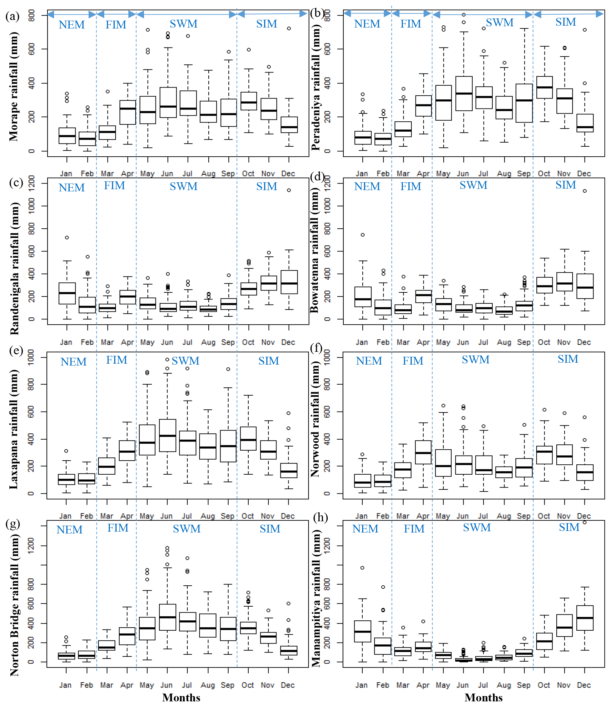
Figure 2Subbasin rainfall for (a) Morape, (b) Peradeniya, (c) Randenigala, (d) Bowatenna, (e) Laxapana, (f) Norwood, (g) Norton Bridge, and (h) Manampitiya. Rainfall seasons are northeastern monsoon (NEM), first inter-monsoon (FIM), southwestern monsoon (SWM), and second inter-monsoon (SIM).
Similar to other investigators, we observe several strong correlations between rainfall anomalies and the climate indices (Tables A1 and A2 and Appendix). Higher correlation values between MEI and rainfall anomalies can be seen compared to the correlation with other ENSO indices (Table 1). In addition, rainfall in the SWM is very important for stations in the humid zone of the country which is the source of a large amount of water stored in reservoirs (Table A2). Correlation coefficients between SWM rainfall at Norton Bridge are negative and strong, −0.31 for MEI (p=0.01) and −0.37 for DMI (p<0.01). The strength of the correlation notwithstanding, the residuals from a regression model indicate that high uncertainty would be associated with any forecast (Fig. 3). Thus, we are led to explore the efficacy of classification methods (Appendix).
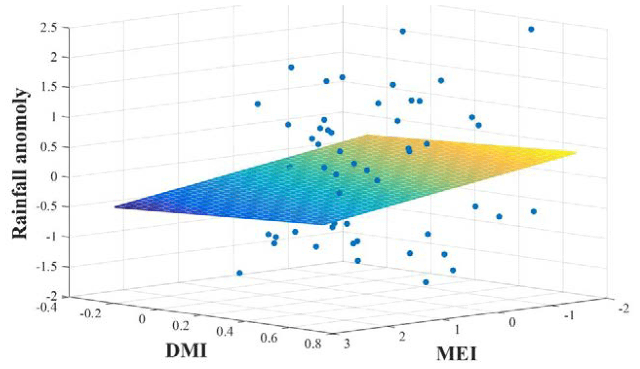
Figure 3Linear regression of rainfall anomaly on MEI and DMI. High values of MEI and DMI are associated with low values of rainfall.
We present classification results for two subbasins, one that has the highest rainfall during the NEM, Manampitiya, and one that has the highest rainfall for the SWM, Norton Bridge (Fig. 4). Norton Bridge represents the areal rainfall of reservoir catchments in the wet zone and Manampitiya represents the rainfall that contributes to irrigation tanks in the dry zone. Results of other subbasins are presented in the Appendix (Figs. A4–A7, Appendix). Because MEI has a higher correlation with rainfall anomalies than other ENSO indices, classification was done with only MEI and MI.
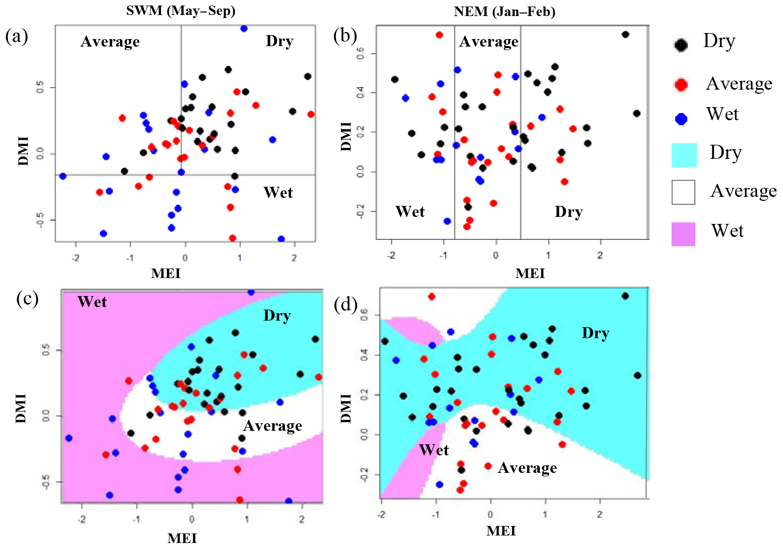
Figure 4Norton Bridge and Manampitiya rainfall classes (dry, average, wet) identified by ENSO and IOD phenomena. (a) Norton Bridge SWM rainfall classification tree model, (b) Manampitiya NEM rainfall classification tree model, (c) Norton Bridge SWM rainfall QDA, and (d) Manampitiya NEM rainfall classification by QDA.
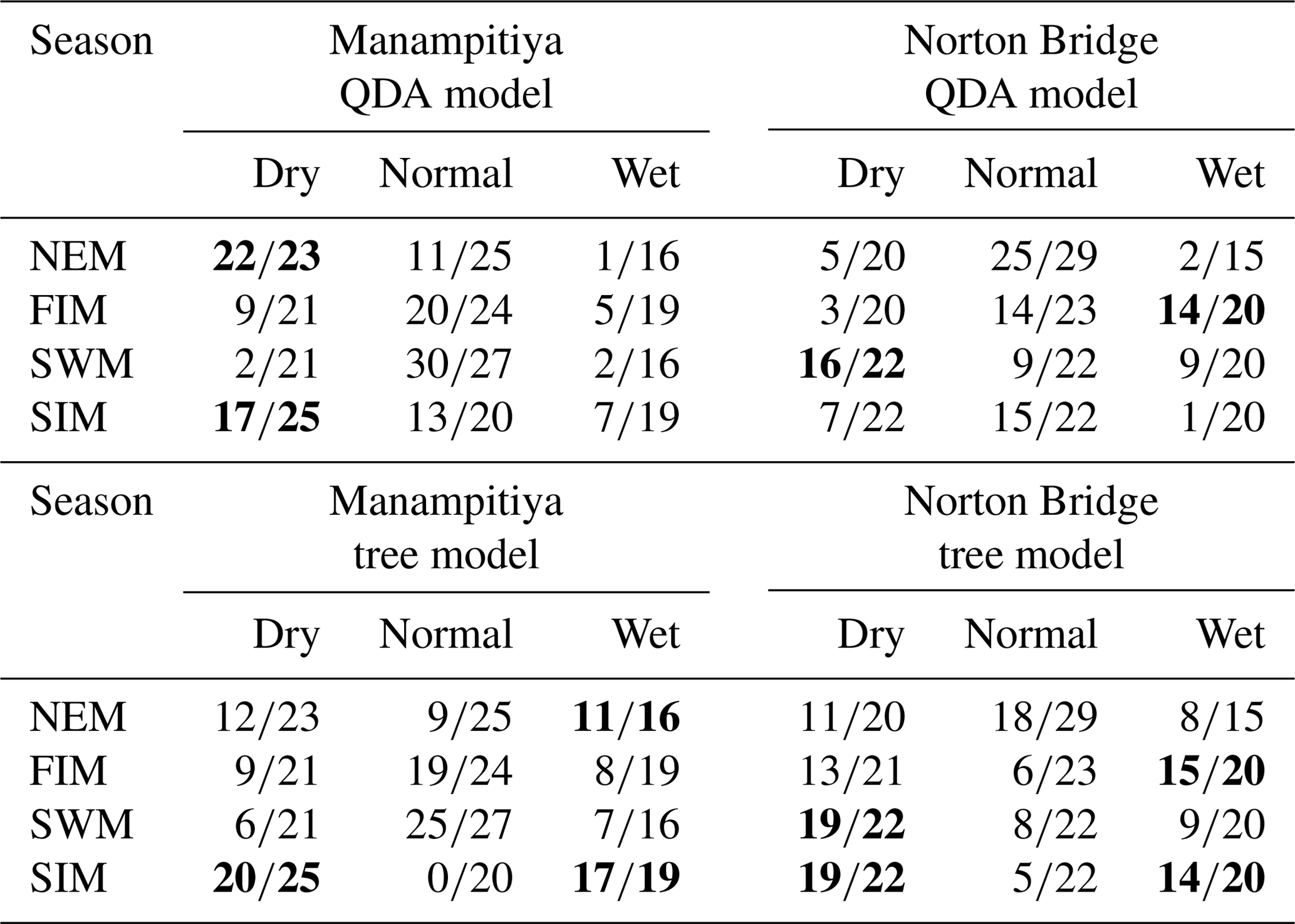
The SWM is a season when the humid zone receives the bulk of rainfall. At Norton Bridge, the occurrences of the dry rainfall anomaly class in the SWM are seen to “clump” in the region of relatively high MEI and DMI. Both the classification tree and the QDA successfully identify the pattern (Fig. 4a and c) with an overall accuracy of 73 %, 19 and 16 correct out of 22 occurrences (Table 2). In the arid zone the NEM season is one of the most important for rainfall. At Manampitiya, the MEI provides the primary variable in the classification, with the dry anomaly class being correctly selected in 52 % by tree model and 95 % with the QDA model. The results suggest that it may be possible to identify seasons when it is expected to be anomalously dry. The correct classification of “average” conditions likely has less importance for water managers. We explored classification using two classes, “dry” and “not dry”. In this case, the classification model again correctly classifies 86 % of the anonymously dry cases and gets more than 69 % of the not dry cases correct (Fig. 5).
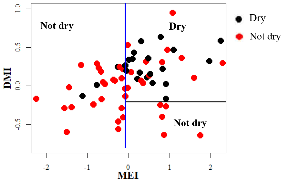
Figure 5Classification tree for Norton Bridge SWM rainfall using two categories (dry and not dry).
Table 2Classification model results. Bold cells indicate where there may be information content with respect to forecasting either dry or wet anomaly classes as judged by a classification success rate of at least two-thirds.
Classification trees are known to be unstable. That is, small changes in the observations can lead to large changes in the decision tree. The random forest approach overcomes the issue by building a “bag” of trees from bootstrap samples. The robustness of the model can then be checked by considering the “out-of-bag” error. The results of the random forest indicate that predictions of three rainfall anomaly classes using MEI and DMI are not feasible (Table 3). The out-of-bag error rate is close to two-thirds, which for three categories is equivalent to a random selection.
Table 3Results of random forest ensemble classification results. Out-of-bag error (OOB) is the classification error calculated from the data not used to fit the tree.
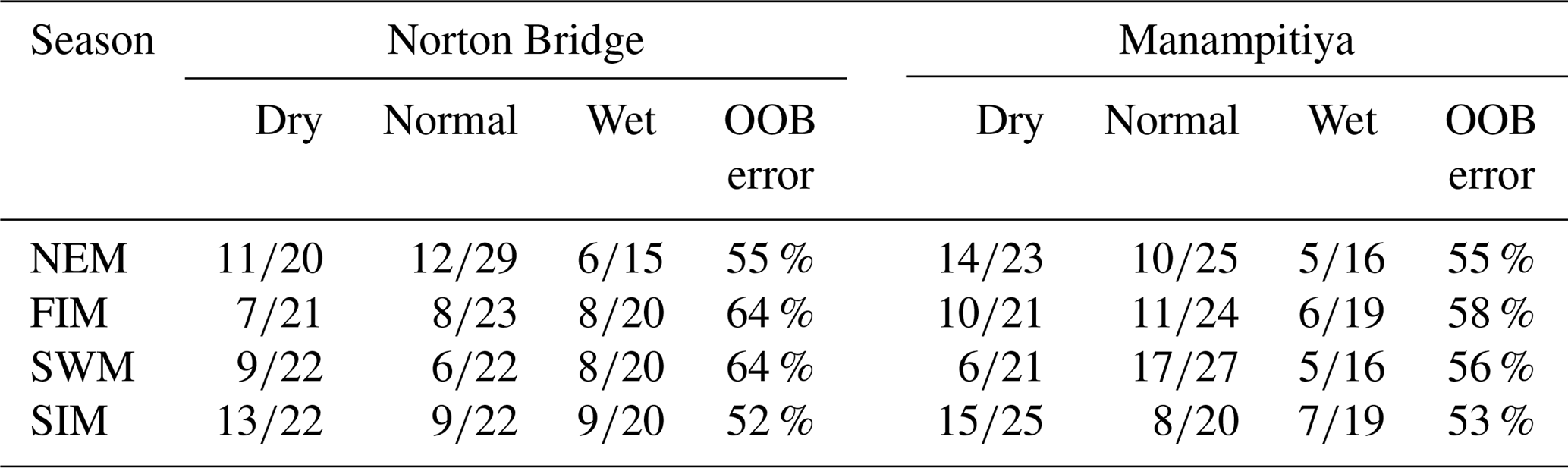
However, the results of the random forest for a classification as either dry or not dry suggest that there may be skill in such a prediction. The out-of-bag error rates for this case range from 22 % to 38 % for Norton Bridge and Manampitiya (Table 3) and from 20 % to 39 % across all stations (Table A7).
Table 4Results of random forest ensemble classification results for two rainfall anomaly classes. Out-of-bag error (OOB) is the classification error calculated from the data not used to fit the tree.

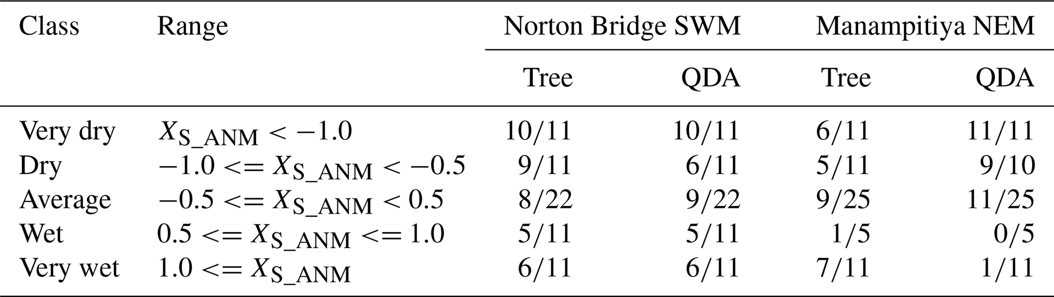
The QDA method produces results that are promising with respect to identification of extreme dry events as indicated by seasonal rainfall (Table 5).
Table 5Classification results for extreme dry (very low rainfall) and wet (very high rainfall) seasons.
Understanding seasonal rainfall variability across the spatially diverse Mahaweli and Kelani River basins is important for irrigation and hydropower water planning. The SWM and SIM are the key rainfall seasons for subbasins in the humid zone (Norton Bridge, Morape, Peradeniya, and Laxapana), delivering 80 % of annual rainfall (Fig. 2a, b, e, f). For the arid zone (Manampitiya) and intermediate zone (Randenigala, Bowatenna) subbasins, the major season is SIM, which delivers more than 40 % of annual rainfall (Fig. 2c, d, h). The arid zone also receives rainfall during the NEM (24 % of annual rainfall at Manampitiya) and the intermediate zone receives rainfall during the SWM (25 %–30 % of annual rainfall at Randenigala and Bowatenna).
Climate teleconnection indices are related to rainfall anomalies observed during the two main growing seasons, Yala and Maha. The Maha agriculture season (October–March) depends on rain from the SIM and NEM. During El Niño events rainfall increases for the first 3 months of the Maha season (SIM: October–December) (Figs. A4, A5, A6, A8) (Ropelewski and Halpert, 1995) and decreases during the last 3 months (NEM: January–March) (Fig. 4b). In the Yala season (April–September), La Niña events enhance the rainfall during the SWM (Figs. 4a, c, A4, A5, A6, A8) (Whitaker et al., 2001). During El Niño events the SWM rainfall is reduced (Figs. 4a, c, A8, A9) (Chandrasekara et.al, 2017; Chandimala and Zubair, 2007; Zubair, 2003). The El Niño impact during the SWM is not as significant as it is during the NEM season (International Research Institute, 2017a). We find, however, that there is an interaction between two teleconnection indices, MEI and IOD for SWM rainfall. During the Yala season there is a high probability of having a drought when both the IOD and MEI are positive (Fig. 5). Also, not having drought is probable when both the IOD and MEI are negative (Figs. 5, A8, A9).
Classification of wet, average, and dry rainfall anomalies using the MEI and DMI indices is successful. For example, a dry SWM season for Norton Bridge (Table 2) and other humid zone stations (Table A4) is classified correctly with greater than 70 % accuracy with QDA and tree models. However, a random forest approach demonstrates that there is little skill in identifying a full wet–average–dry classification. However, a random forest model using only two rainfall categories shows more than 60 % accuracy in identifying dry and not dry classes of key rainfall seasons of the humid zone (Tables 4 and A7). Similarly, for arid zone locations such as Manampitiya, the dry rainfall class identification for NEM and SIM seasons is about 60 % (Tables 4 and A7).
Our statistical classification models can be combined with MEI and DMI forecasts to indicate the season-ahead expectation for rainfall. ENSO forecasts are available from the International Research Institute for Climate and Society (International Research Institute, 2017b) and IOD forecasts are available in the Bureau of Meteorology (BOM), Australian Government (Bureau of Meteorology, 2017). ENSO and IOD predictions are also associated with the uncertainty. Therefore, final forecast accuracy is a combination of the MEI, DMI forecast uncertainties, and model's accuracy rate in each class. Although overall prediction accuracy is not extremely high, a forecast of an anomalously low rainfall season can have value for risk-averse farmers (Cabrera et al., 2007) and can guide plans for hydropower management (Block and Goddard, 2012).
The electricity and agriculture sectors of Sri Lanka heavily rely on Mahaweli and Kelani River water resources so season-ahead forecasts of abnormally low rainfall should be useful for decisions on adaptation measures. For example, water availability of the first 3 months of a growing season is important for crop selection and the extent of land to be cultivated. Hydropower planning and scheduling of maintenance of the power plants can also benefit from season-ahead forecasts. The damage that can occur due to incorrect rainfall forecasts in the agriculture and energy sectors can be minimized with emergency planning during the season, which is the usual practice.
Although the accuracy of predicting low or not low seasonal rainfall is not very high, decisions based on forecasts that are improvements over climate averages should be an improvement over current practices. The accuracy of statistical models can be improved with longer records, which are important to train the classification models. Also, models can be fine-tuned for important shorter periods such as crop planting months and harvesting months for irrigation water planning.
ENSO and IOD phenomena teleconnections with river basin rainfall provide potentially useful information for water resource management. Relationships identified between teleconnection indices and river basin rainfall agree with other research findings. Prediction of seasonal rainfall classes from ENSO and IOD indices can inform water resource managers in reservoir operation planning for both hydropower and irrigation releases.
Codes use for the analysis and generating the graphs can be found at https://github.com/thusharadesilva/Rainfall_Season_Classification.git (De Silva M., 2019).
Areal rainfall data can be found from Ceylon Electricity Board or Mahaweli Authority of Sri Lanka. It is required to obtain the data from either of these organization and it is not possible to make the data publically available. We added data of one station with the codes to test the codes; however, the name is not mentioned to protect the privacy. Climate index data are publically available and references are given.
-
DMI data: Japan Agency for Marine Earth Science and Technology: SST/DMI data set;
-
MEI data: National Oceanic and Atmospheric Administration: El Niño–Southern Oscillation;
-
NINO3, NINO3.4, NINO4 data: National Center for Atmospheric Research: NINO SST indices (NINO 1+2, 3, 3.4, 4; ONI and TNI).
A1 Normality testing
The Shapiro–Wilk's method is used to identify the normality of rainfall
anomaly distribution. The Manampitiya NEM normality test results are given
below as an example.
| Data 1: original data |
| W=0.96675, p value = 0.08185 |
| Data 2: data transformed by square root |
| W=0.98772, p value = 0.7772 |
| Data 3: data transformed by log |
| W=0.91577, p value = 0.0003325 |
Further, from data plots (Fig. A1) and the S-W statistic, we conclude that the square root transformed data are closer to being normally distributed than the other forms.
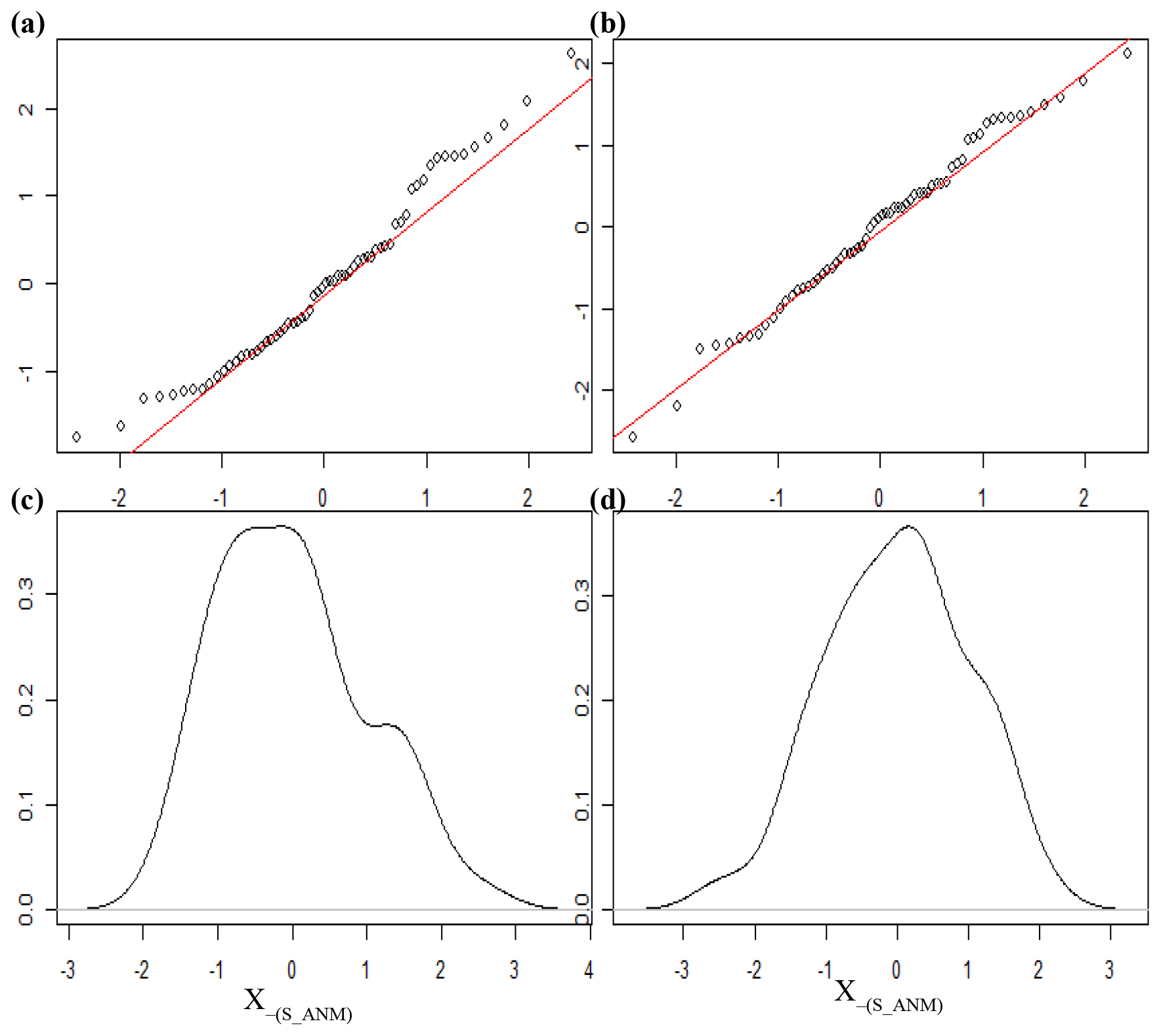
Figure A1Manampitiya NEM standardized data. (a) Original form qqplot, (b) square root form qqplot, (c) original form density plot, and (d) square root form density plot.
A2 Classification of data
Using 0.5 as a threshold for a normal distribution defines portions of the data that are fairly evenly distributed into three categories – about 31 %, 38 %, and 31 % for a normal distribution (Fig. A2). We deemed this a reasonable choice for our analysis.
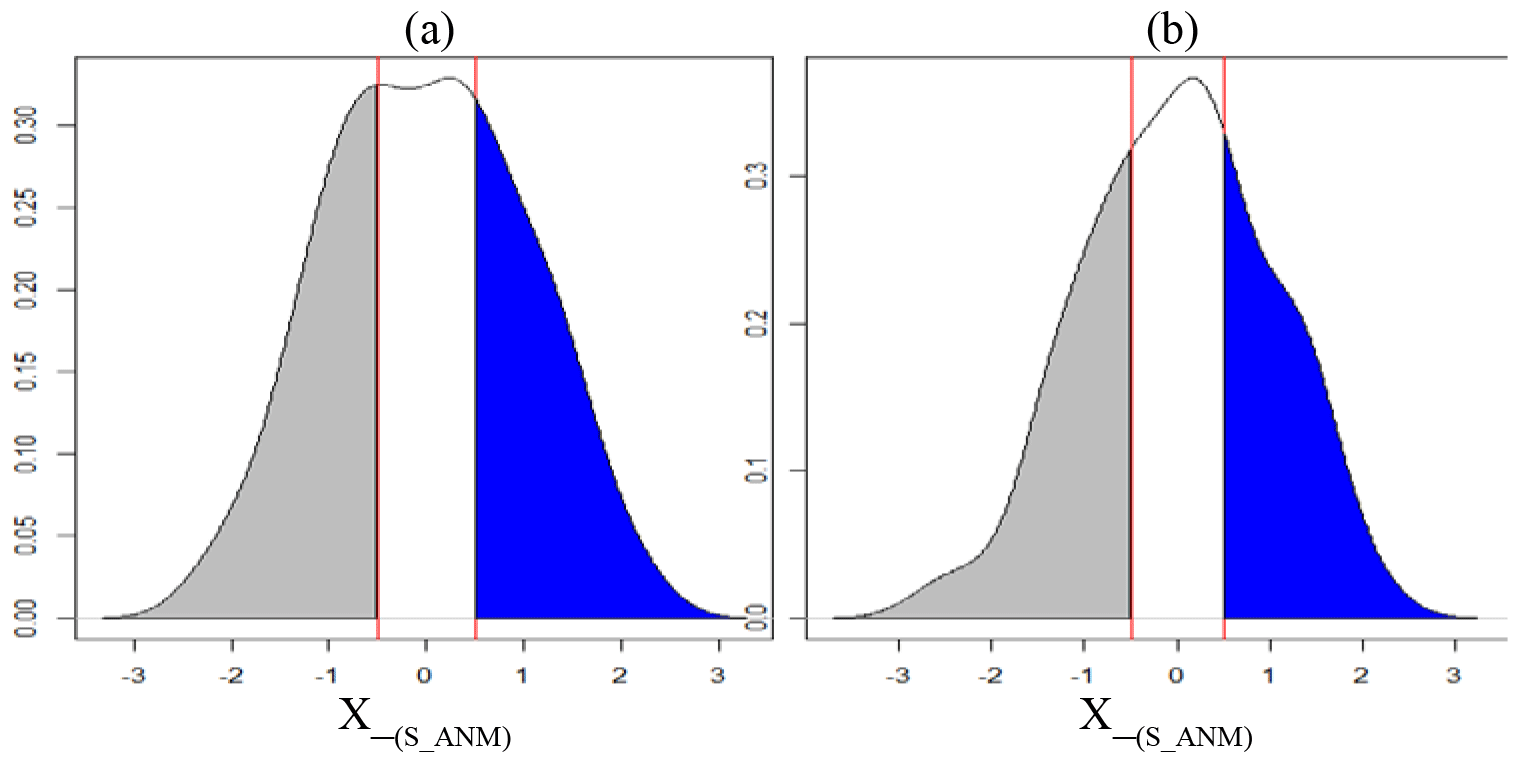
Figure A2(a) Norton Bridge SWM rainfall anomaly distribution; (b) Manampitiya NEM rainfall anomaly distribution.
A3 Correlation analysis with multiple climate indices
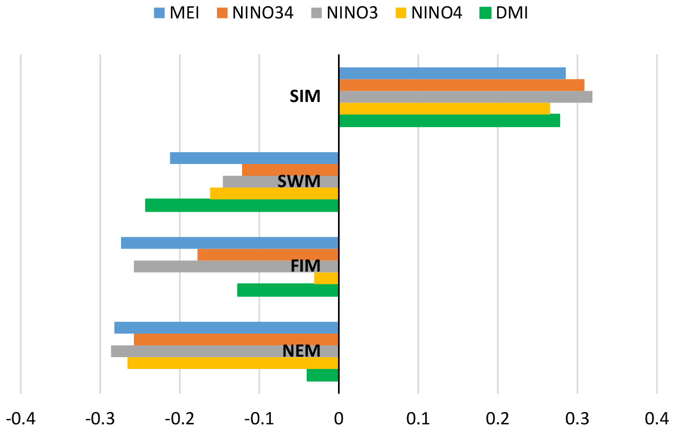
We examined the correlation between rainfall anomalies and multiple climate indices to choose the two climate indices MEI and DMI (Fig. A3, Table A1). The ENSO phenomenon is represented by MEI, NINO34, NINO3, and NINO4 indices. Correlation analysis indicates that MEI, which is estimated using several climate factors such as sea-level pressure, zonal and meridional components of the surface wind, sea surface temperature, surface air temperature, and total cloudiness fraction of the sky (National Oceanic and Atmospheric Administration, 2017), demonstrates higher correlation with rainfall anomalies in subbasins for all rainfall seasons compared to NINO34, NINO3, and NINO4. The Indian Ocean dipole phenomenon is represented by the DMI index, which represents the gradient of the sea surface temperature. Based on the correlation analysis and the content of the indices, we selected MEI as the indicator for ENSO and DMI as the indicator for IOD.
A4 Correlation analysis with MEI and DMI climate indices
Correlation coefficients between rainfall anomalies and MEI and DMI are negative for the NEM, FIM, and SWM seasons and positive for the SIM season. Rainfall anomaly correlations to the DMI are not stronger than the correlations to the MEI. However, there are strong correlations for the anomalies of major monsoons to the subbasins and DMI values. For example, wet subbasins (Morape, Peradeniya, Laxapana, Norwood, Norton Bridge) have a high correlation coefficient between SWM rainfall anomalies and DMI, while dry zone (Manampitiya) and intermediate zone (Randenigala, Bowatenna) subbasins have a high correlation coefficient between NEM and SIM rainfall anomalies.
Classification method classification tree models, random forest, and quadratic discriminant analysis identify the relationship between standardized rainfall anomaly classes (dry, average, wet) and MEI and DMI values (Figs. A4–A7). Positive values of MEI and DMI values resulted in dry or average rainfall class for the NEM, FIM, and SWM seasons. However, for SIM rainfall has wet or average class for the positive values of MEI and DMI. The accuracy of model results is high for the dominant monsoon rainfall seasons of each subbasin (Tables A3–A5). The ensemble model approach with random forest has given a comparatively lower out-of-bag error rate for the dominant monsoons' rainfall anomaly classification (Table A5). For example, for wet zone subbasins such as Norton Bridge, Norwood, Laxapana, Peradeniya, and Morape random forest error rate is lower for the SWM and SIM seasons. Similarly, for dry and intermediate subbasins Manampitiya, Randenigala, and Bowatenna the NEM and SIM rainfall classes' accuracy rate is higher than other rainfall seasons. Also, all three models have a higher accuracy rate in identifying dry events, and the error rate of identifying wet and dry class is also less than 15 % (Tables A3–A5). Further analysis of the two dry and not dry rainfall classes is relevant to the MEI and DMI values with classification tree and random forest methods (Figs. A8 and A9). Classification tree models for two classes have a higher accuracy rate of 65 %–84 % for eight subbasins (Table A6). Random forest out-of-bag error for the two class models varies between 20 % and 39 % and shows higher skill in identifying rainfall classes for major monsoons of the subbasins (Table A7). MEI shows higher variable importance of identifying the rainfall classes compared to the DMI values. In particular, for NEM and SIM, which are important to the dry zone subbasins, importance of MEI is high in the classification. However, some of the wet zone subbasins show equal importance of the DMI variable in identifying two rainfall classes in FIM and SWM (Fig. A10).
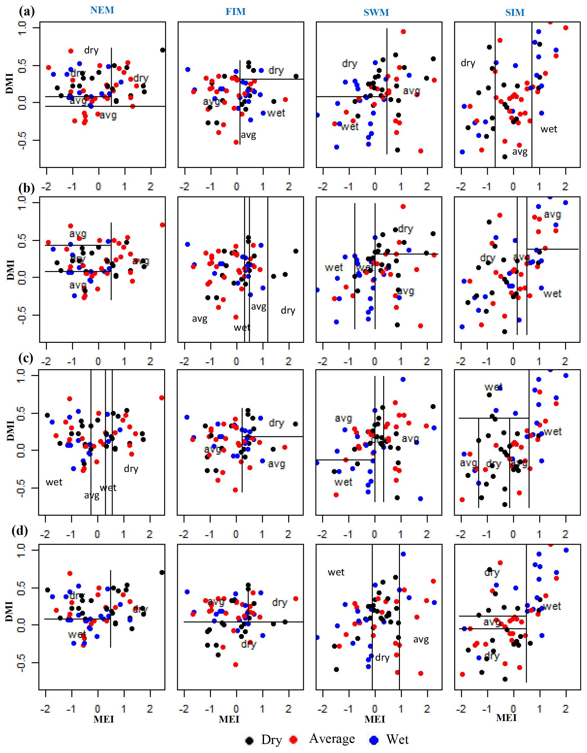
Figure A4Identifying relationships between three rainfall classes (dry, average, wet) and MEI and DMI values using classification tree models. (a) Morape, (b) Peradeniya, (c) Randenigala, and (d) Bowatenna.
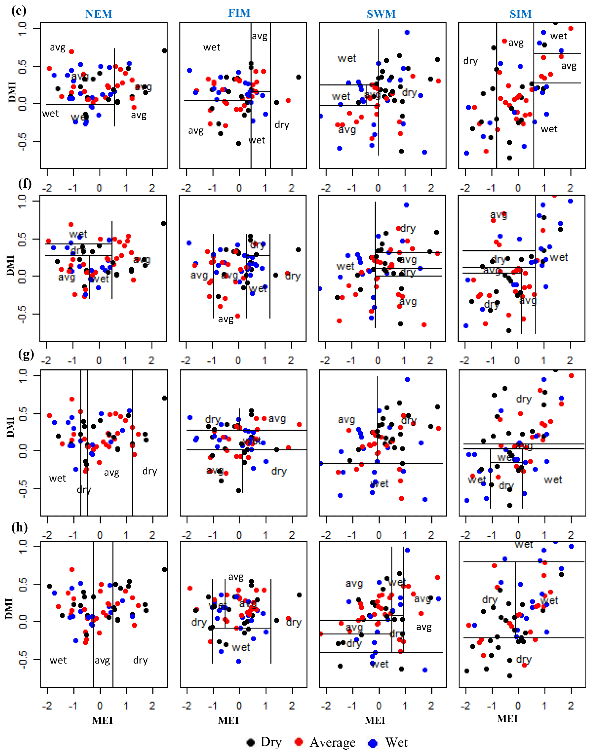
Figure A5Identifying relationships between three rainfall classes (dry, average, wet) and MEI and DMI values using classification tree models. (a) Laxapana, (b) Norwood, (c) Norton Bridge, and (d) Manampitiya.
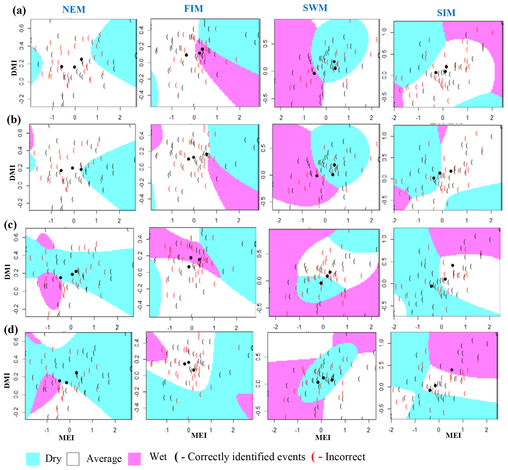
Figure A6Identifying relationships between three rainfall cases (dry, average, wet) and MEI and DMI values using QDA models. (a) Morape, (b) Peradeniya, (c) Randenigala, and (d) Bowatenna.

Figure A7Identifying relationships between three rainfall classes (dry, average, wet) and MEI and DMI values using classification tree models. (e) Laxapana, (f) Norwood, (g) Norton Bridge, and (h) Manampitiya.
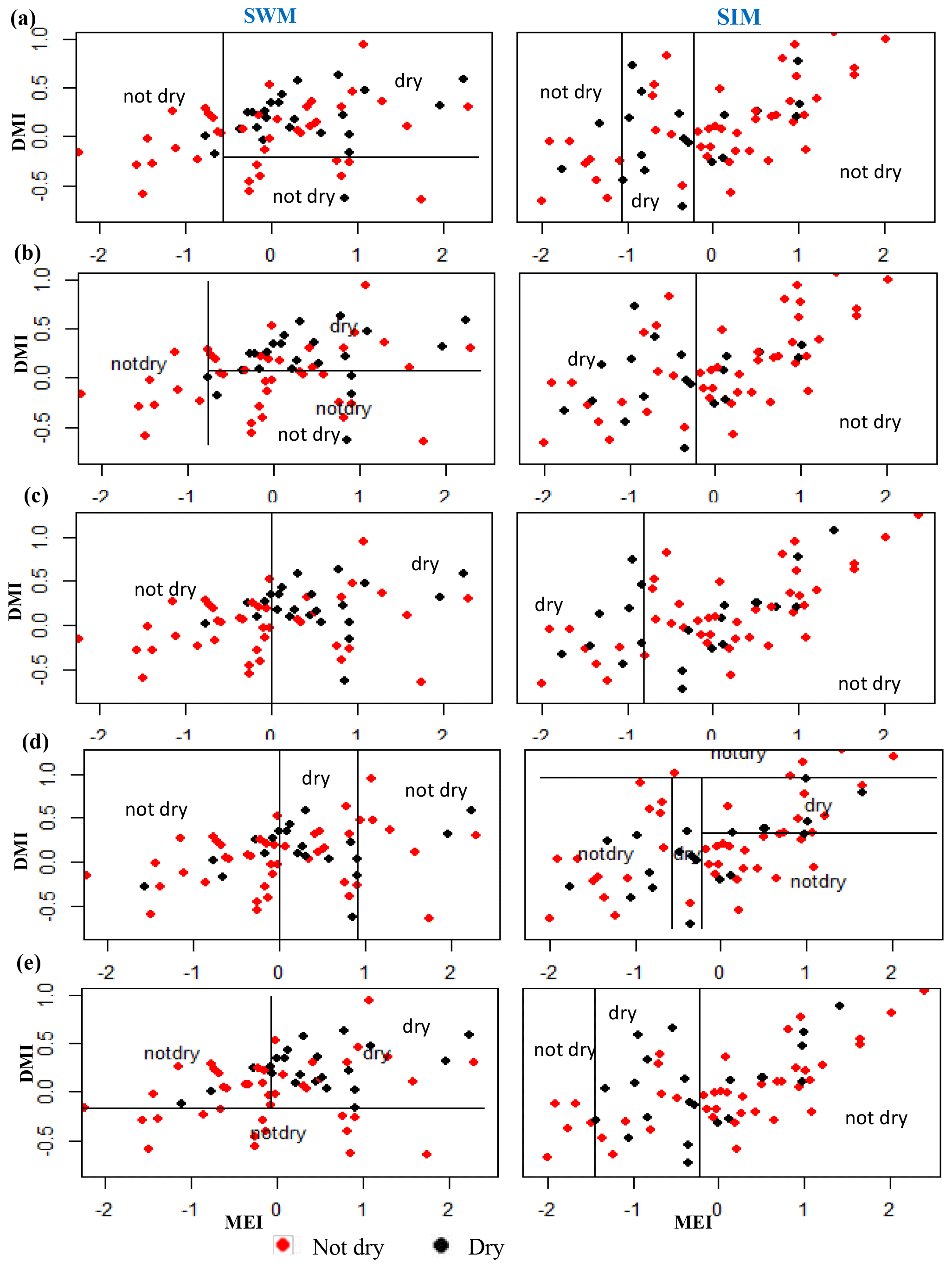
Figure A8Identifying relationships between two rainfall classes (dry, not dry) and MEI and DMI values using classification tree models for dry and intermediate zone subbasins for the NEM and SIM seasons. (f) Randenigala, (g) Bowatenna, and (h) Manampitiya.

Figure A9Random forest importance of variables to identify the dry and not dry classes of rainfall anomalies.
Table A1Correlation analysis of rainfall anomalies and climate indices.
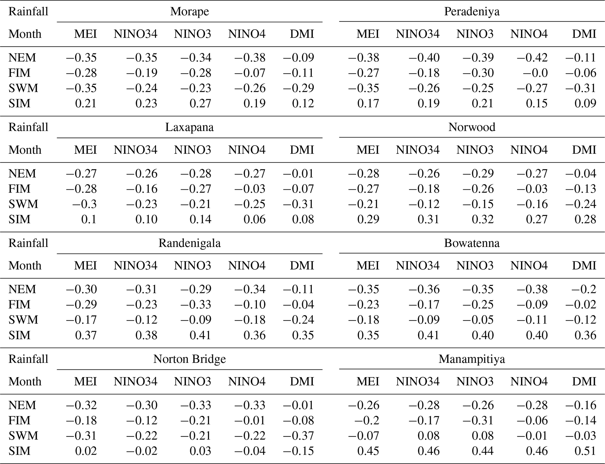
Table A2Correlation between rainfall anomalies and MEI and DMI indices. High correlation coefficients are highlighted.
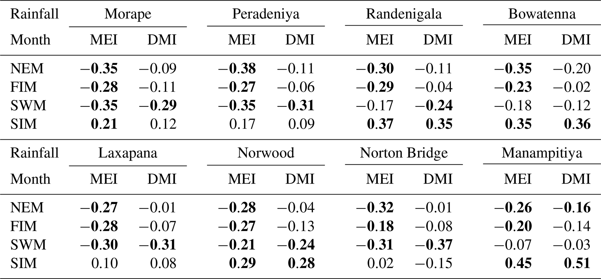
Table A3Classification tree model results. Highlighted cells indicate where there may be information content with respect to forecasting either dry or wet anomaly classes.

Table A4Classification QDA model results. Highlighted cells indicate where there may be information content with respect to forecasting either dry or wet anomaly classes.
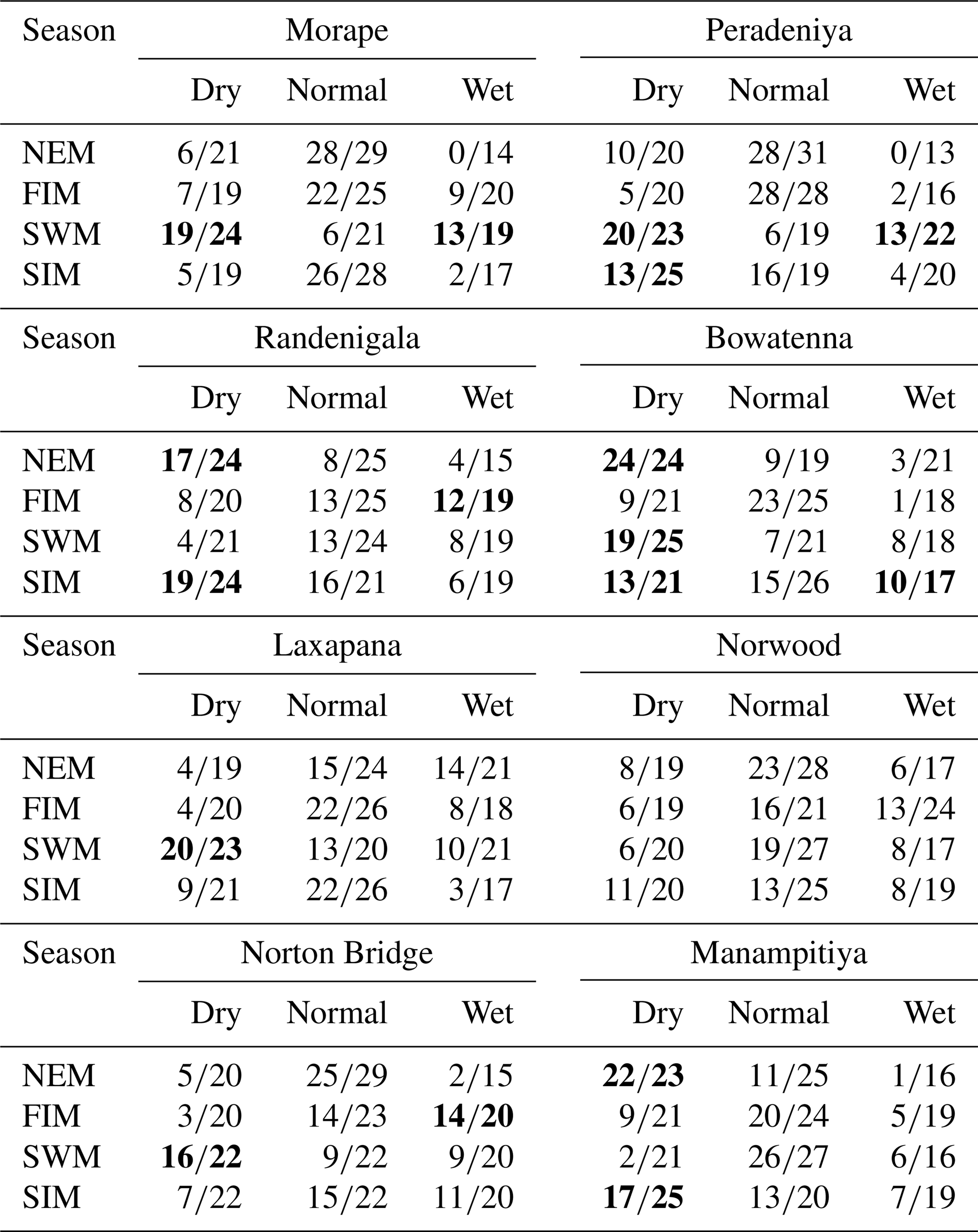
Table A5Random forest model results. Highlighted cells indicate where there may be information content with respect to forecasting either dry or wet anomaly classes.

Table A6Classification tree model results for major rainfall season in the subbasins.


TDM and GMH conceptualized the study and TDM carried out the data analysis. TDM prepared the paper with contribution from GMH.
The authors declare that they have no conflict of interest.
This research is part of a multidisciplinary research initiative called Agricultural Decision-Making and Adaptation to Precipitation Trends in Sri Lanka (ADAPT-SL) at Vanderbilt Institute for Energy and Environment (VIEE). The work is supported by WSC program grant no. NSF-EAR 1204685.
This paper was edited by Wouter Buytaert and reviewed by two anonymous referees.
Amarasekera, K. N., Lee, R. F., Williams, E. R., and Eltahir, E. A. B.: ENSO and the natural variability in the flow tropical rivers, J. Hydrol., 200, 24–39, https://doi.org/10.1016/S0022-1694(96)03340-9, 1997.
Analytical Vidhya Team: Tunning the parameters of your Random Forest model, available at: https://www.analyticsvidhya.com/blog/2015/06/tuning-random-forest-model/ (last access: 12 March 2018), 2015.
Analytical Vidhya Team: A Complete Tutorial on Tree Based Modeling from Scratch, available at: https://www.analyticsvidhya.com/blog/2016/04/complete-tutorial-tree-based-modeling-scratch-in-python/ (last access: 12 March 2018), 2016.
Block, P. and Goddard, L.: Statistical and Dynamical Climate Predictions to Guide Water Resources in Ethiopia, J. Water Resour. Plan. Manage., 138, 287–298, https://doi.org/10.1061/(ASCE)WR.1943-5452.0000181, 2012.
Breiman, L.: Randomforest2001, Mach. Learn., 45, 5–32, https://doi.org/10.1017/CBO9781107415324.004, 2001.
Bureau of Meteorology: Record-breaking La Niña events, Bureau of Meteorology, 26, available at: http://www.bom.gov.au/climate/enso/history/La-Nina-2010-12.pdf (last access: 1 February 2018), 2012.
Bureau of Meteorology: Indian Ocean, POAMA monthly mean IOD forecast, available at: http://www.bom.gov.au/climate/enso/#tabs=Indian-Ocean, last access: 30 March 2017.
Cabrera, V. E., Letson, D., and Podesta, G.: The value of climate information when farm programs matter, Agricult. Syst., 93, 25–42, https://doi.org/10.1016/j.agsy.2006.04.005, 2007.
Cao, Q., Hao, Z., Yuan, F., Su, Z., Berndtsson, R., Hao, J., and Nyima, T.: Impact of ENSO regimes on developing- and decaying-phase precipitation during rainy season in China, Hydrol. Earth Syst. Sci., 21, 5415–5426, https://doi.org/10.5194/hess-21-5415-2017, 2017.
Ceylon Electricity Board: Long Term Generation Expansion Plan 2015–2034, available at: http://pucsl.gov.lk/english/wp-content/uploads/2015/09/Long-Term-Generation-Plan-2015-2034-PUCSL.pdf (last access: 1 September 2017), 2015.
Ceylon Electricity Board: River Basin Hydrology Data, System control branch Transmission Division, Sri Lanka, 2017.
Chandimala, J. and Zubair, L.: Predictability of stream flow and rainfall based on ENSO for water resources management in Sri Lanka, J. Hydrol., 335, 303–312, https://doi.org/10.1016/j.jhydrol.2006.11.024, 2007.
Chandrasekara, S., Prasanna, V., and Kwon, H. H.: Monitoring Water Resources over the Kotmale Reservoir in Sri Lanka Using ENSO Phases, Adv. Meteorol., 2017, 4025964, https://doi.org/10.1155/2017/4025964, 2017.
Chaudhari, H. S., Pokhrel, S., Mohanty, S., and Saha, S. K.: Seasonal prediction of Indian summer monsoon in NCEP coupled and uncoupled model, Theor. Appl. Climatol., 114, 459–477, https://doi.org/10.1007/s00704-013-0854-8, 2013.
Denise, C., Rogers, W., and Beringer, J.: Describing rainfall in northern Australia using multiple climate indices, Biogeosciences, 14, 597–615, https://doi.org/10.5194/bg-14-597-2017, 2017.
Department of Agriculture Sri Lanka: Climate zones of Sri Lanka, available at: https://www.doa.gov.lk/images/weather_climate/Climatezone.jpg, last access: 7 November 2017.
Department of Meteorology Sri Lanka: Climate of Sri Lanka., available at: http://www.meteo.gov.lk/index.php?option=com_content&view=article&id=94&Itemid=310&lang=en, last access: 7 November 2017.
De Silva M., T.: Rainfall_Season_Classification, available at: https://github.com/thusharadesilva/Rainfall_Season_Classification.git, last access: 28 March 2019.
Dettinger, M. D. and Diaz, H. F.: Global Characteristics of Stream Flow Seasonality and Variability, J. Hydrometeorol., 1, 289–310, https://doi.org/10.1175/1525-7541(2000)001<0289:GCOSFS>2.0.CO;2, 2000.
Easterling, D. R., Meehl, G. A., Parmesan, C., Changnon, S. A., Karl, T. R., and Mearns, L. O.: Climate extremes: Observations, modeling, and impacts, Science, 289, 2068–2074, https://doi.org/10.1126/science.289.5487.2068, 2000.
Eden, J. M., Van Oldenborgh, G. J., Hawkins, E., and Suckling, E. B.: A global empirical system for probabilistic seasonal climate prediction, Geosci. Model Dev., 8, 3947–3973, https://doi.org/10.5194/gmd-8-3947-2015, 2015.
Gerlitz, L., Vorogushyn, S., Apel, H., Gafurov, A., Unger-Shayesteh, K., and Merz, B. A.: Statistically based seasonal precipitation forecast model with automatic predictor selection and its application to central and south Asia, Hydrol. Earth Syst. Sci., 20, 4605–4623, https://doi.org/10.5194/hess-20-4605-2016, 2016.
International research institute: ENSO resources, El-Nino teleconnections & La-Nina teleconnections, available at: http://iri.columbia.edu/our-expertise/climate/enso/ (last access: 1 January 2017), 2017a.
International research institute: IRI ENSO forecast, available at: http://iri.columbia.edu/our-expertise/climate/forecasts/enso/current (last access: 1 January 2017), 2017b.
International Research Institute for Climate Society: IRI Seasonal Precipitation Forecast, available at: http://iridl.ldeo.columbia.edu/maproom/Global/Forecasts/NMME_Seasonal_Forecasts/Precipitation_ELR.html, last access: 12 February 2018.
James, G., Witten, D., Hastie, T., and Tibshirani, R.: An introduction to statistical learning., in: Vol. 112, Springer, New York, p. 18, ISBN 978-1-4614-7138-7, https://doi.org/10.1007/978-1-4614-7138-7, 2013.
Japan Agency for Marine Earth Science and Technology: SST/DMI data set, available at: http://www.jamstec.go.jp/aplinfo/sintexf/DATA/dmi.monthly.txt, last access: 1 February 2019.
Jentsch, A., Kreyling, J., and Beierkuhnlein, C.: A new generation of events, not trends experiments, Front. Ecol. Environ., 5, 365–374, https://doi.org/10.1890/1540-9295(2007)5[365:ANGOCE]2.0.CO;2, 2007.
Jha, S., Sehgal, V. K., Raghava, R., and Sinha, M.: Teleconnections of ENSO and IOD to summer monsoon and rice production potential of India, Dynam. Atmos. Oceans, 76, 93–104, https://doi.org/10.1016/j.dynatmoce.2016.10.001, 2016.
Knapp, A. K., Hoover, D. L., Wilcox, K. R., Avolio, M. L., Koerner, S. E., La Pierre, K. J., and Smith, M. D.: Characterizing differences in precipitation regimes of extreme wet and dry years: Implications for climate change experiments, Global Change Biol., 21, 2624–2633, https://doi.org/10.1111/gcb.12888, 2015.
Korecha, D. and Sorteberg, A.: Validation of operational seasonal rainfall forecast in Ethiopia, Water Resour. Res., 49, 7681–7697, https://doi.org/10.1002/2013WR013760, 2013.
Lee, H.: General Rainfall Patterns in Indonesia and the Potential Impacts of Local Seas on Rainfall Intensity, Water, 7, 1751–1769, https://doi.org/10.3390/w7041751, 2015.
Löwe, R., Madsen, H., and McSharry, P.: Objective classification of rainfall in northern Europe for online operation of urban water systems based on clustering techniques, Water (Switzerland), 8, 87, https://doi.org/10.3390/w8030087, 2016.
Maity, R. and Nagesh Kumar, D.: Bayesian dynamic modeling for monthly Indian summer monsoon rainfall using El Niño-Southern Oscillation (ENSO) and Equatorial Indian Ocean Oscillation (EQUINOO), J. Geophys. Res.-Atmos., 111, 1–12, https://doi.org/10.1029/2005JD006539, 2006.
Malmgren, B. A., Hulugalla, R., Hayashi, Y., and Mikami, T.: Precipitatioon trends in Sri Lanka since the 1870s and relationships to El Niño-southern oscillation, Int. J. Climatol., 23, 1235–1252, https://doi.org/10.1002/joc.921, 2003.
Malmgren, B. A., Hullugalla, R., Lindeberg, G., Inoue, Y., Hayashi, Y., and Mikami, T.: Oscillatory behavior of monsoon rainfall over Sri Lanka during the late 19th and 20th centuries and its relationships to SSTs in the Indian Ocean and ENSO, Theor. Appl. Climatol., 89, 115–125, https://doi.org/10.1007/s00704-006-0225-9, 2007.
Manchanayake, P. and Madduma Bandara, C.: Water Resources of Sri Lanka, National Science Foundation, Sri Lanka, available at: http://thakshana.nsf.ac.lk/slstic/NA-202/NA_202.pdf (last access: 1 August 2017), 1999.
National Center for Atmospheric Research: NINO SST Indices (NINO 1+2, 3, 3.4, 4; ONI and TNI), available at: https://climatedataguide.ucar.edu/climate-data/nino-sst-indices-nino-12-3-34-4-oni-and-tni, last access: 1 February 2018.
National Oceanic and Atmospheric Administration: El Nino Southern oscilation, available at: http://www.esrl.noaa.gov/psd/enso/past_events.html (last access: 1 August 2018), 2017.
National Oceanic and Atmospheric Administration: Three Months Outlook, Official Forecast, Climate Prediction Center, National Weather Services, available at: http://www.cpc.ncep.noaa.gov/products/predictions/long_range/seasonal.php?lead=6, last access: 12 February 2018.
Nur'utami, M. N. and Hidayat, R.: Influences of IOD and ENSO to Indonesian Rainfall Variability: Role of Atmosphere-ocean Interaction in the Indo-pacific Sector, Proced. Environ. Sci., 33, 196–203, https://doi.org/10.1016/j.proenv.2016.03.070, 2016.
Ouyang, R., Liu, W., Fu, G., Liu, C., Hu, L., and Wang, H.: Linkages between ENSO/PDO signals and precipitation, streamflow in China during the last 100 years, Hydrol. Earth Syst. Sci., 18, 3651–3661, https://doi.org/10.5194/hess-18-3651-2014, 2014.
Power, S., Casey, T., Folland, C., Colman, A., and Mehta, V.: Inter-decadal modulation of the impact of ENSO on Australia, Clim. Dynam., 15, 319–324, https://doi.org/10.1007/s003820050284, 1999.
Qiu, Y., Cai, W., Guo, X., and Ng, B.: The asymmetric influence of the positive and negative IOD events on China's rainfall, Scient. Rep., 4, 4943, https://doi.org/10.1038/srep04943, 2014.
Ranatunge, E., Malmgren, B. A., Hayashi, Y., Mikami, T., Morishima, W., Yokozawa, M., and Nishimori, M.: Changes in the Southwest Monsoon mean daily rainfall intensity in Sri Lanka: Relationship to the El Niño-Southern Oscillation, Palaeogeogr. Palaeocl., 197, 1–14, https://doi.org/10.1016/S0031-0182(03)00383-3, 2003.
Reason, C. J. C., Landman, W., and Tennant, W.: Seasonal to decadal prediction of southern African climate and its links with variability of the Atlantic ocean, B. Am. Meteorol. Soc., 87, 941–955, https://doi.org/10.1175/BAMS-87-7-941, 2006.
Ropelewski, C. F. and Halpert, M. S.: Quantifying Southern Oscillation–Precipitation Relantionships, J. Climate, 9, 1043–1059, 1996.
Schneider, T., Bischoff, T., and Haug, G. H.: Migrations and dynamics of the intertropical convergence zone, Nature, 513, 45–53, https://doi.org/10.1038/nature13636, 2014.
Seibert, M., Merz, B., and Apel, H.: Seasonal forecasting of hydrological drought in the Limpopo Basin: A comparison of statistical methods, Hydrol. Earth Syst. Sci., 21, 1611–1629, https://doi.org/10.5194/hess-21-1611-2017, 2017.
Singhrattna, N., Rajagopalan, B., Clark, M., and Kumar, K. K.: Seasonal forecasting of Thailand summer monsoon rainfall, Int. J. Climatol., 25, 649–664, https://doi.org/10.1002/joc.1144, 2005a.
Singhrattna, N., Rajagopalan, B., Krishna Kumar, K., and Clark, M.: Interannual and interdecadal variability of Thailand summer monsoon season, J. Climate, 18, 1697–1708, https://doi.org/10.1175/JCLI3364.1, 2005b.
Smith, M. D.: The ecological role of climate extremes: Current understanding and future prospects, J. Ecol., 99, 651–655, https://doi.org/10.1111/j.1365-2745.2011.01833.x, 2011.
Suppiah, R.: Spatial and temporal variations in the relationships between the southern oscillation phenomenon and the rainfall of Sri Lanka, Int. J. Climatol., 16, 1391–1407, https://doi.org/10.1002/(SICI)1097-0088(199612)16:12<1391::AID-JOC94>3.0.CO;2-X, 1996.
Surendran, S., Gadgil, S., Francis, P. A., and Rajeevan, M.: Prediction of Indian rainfall during the summer monsoon season on the basis of links with equatorial Pacific and Indian Ocean climate indices, Environ. Res. Lett., 10, 094004, https://doi.org/10.1088/1748-9326/10/9/094004, 2015.
Verdon, D. C. and Franks, S. W.: Indian Ocean sea surface temperature variability and winter rainfall: Eastern Australia, Water Resour. Res., 41, 1–10, https://doi.org/10.1029/2004WR003845, 2005.
Ward, P. J., Eisner, S., Flo Rke, M., Dettinger, M. D., and Kummu, M.: Annual flood sensitivities to el nintild;O-Southern Oscillation at the global scale, Hydrol. Earth Syst. Sci., 18, 47–66, https://doi.org/10.5194/hess-18-47-2014, 2014.
Whitaker, D. W., Wasimi, S. A., and Islam, S.: The El Niño – Southern Oscillation and Long-Range the Forecastong of Flows in the Ganges, Int. J. Climatol., 21, 77–87, 2001.
Zubair, L.: El Niño-southern oscillation influences on the Mahaweli streamflow in Sri Lanka, Int. J. Climatol., 23, 91–102, https://doi.org/10.1002/joc.865, 2003.
Zubair, L. and Ropelewski, C. F.: The strengthening relationship between ENSO and northeast monsoon rainfall over Sri Lanka and southern India, J. Climate, 19, 1567–1575, https://doi.org/10.1175/JCLI3670.1, 2006.
- Abstract
- Introduction
- Hydrometeorology and climatology of the study area
- Methods
- Results
- Discussion
- Conclusion
- Code availability
- Data availability
- Appendix A: Identifying ENSO influences on rainfall with classification models: implications for water resource management of Sri Lanka
- Author contributions
- Competing interests
- Acknowledgements
- Review statement
- References