Comparative analyses of hydrological responses of two adjacent watersheds to climate variability and change using the SWAT model

Water quality problems in the Chesapeake Bay Watershed (CBW) are expected to be exacerbated by climate variability and change. However, climate impacts on agricultural lands and resultant nutrient loads into surface water resources are largely unknown. This study evaluated the impacts of climate variability and change on two adjacent watersheds in the Coastal Plain of the CBW, using the Soil and Water Assessment Tool (SWAT) model. We prepared six climate sensitivity scenarios to assess the individual impacts of variations in CO₂ concentration (590 and 850 ppm), precipitation increase (11 and 21 %), and temperature increase (2.9 and 5.0 ^∘C), based on regional general circulation model (GCM) projections. Further, we considered the ensemble of five GCM projections (2085–2098) under the Representative Concentration Pathway (RCP) 8.5 scenario to evaluate simultaneous changes in CO₂, precipitation, and temperature. Using SWAT model simulations from 2001 to 2014 as a baseline scenario, predicted hydrologic outputs (water and nitrate budgets) and crop growth were analyzed. Compared to the baseline scenario, a precipitation increase of 21 % and elevated CO₂ concentration of 850 ppm significantly increased streamflow and nitrate loads by 50 and 52 %, respectively, while a temperature increase of 5.0 ^∘C reduced streamflow and nitrate loads by 12 and 13 %, respectively. Crop biomass increased with elevated CO₂ concentrations due to enhanced radiation- and water-use efficiency, while it decreased with precipitation and temperature increases. Over the GCM ensemble mean, annual streamflow and nitrate loads showed an increase of ∼ 70 % relative to the baseline scenario, due to elevated CO₂ concentrations and precipitation increase. Different hydrological responses to climate change were observed from the two watersheds, due to contrasting land use and soil characteristics. The watershed with a larger percent of croplands demonstrated a greater increased rate of 5.2 kg N ha⁻¹ in nitrate yield relative to the watershed with a lower percent of croplands as a result of increased export of nitrate derived from fertilizer. The watershed dominated by poorly drained soils showed increased nitrate removal due do enhanced denitrification compared to the watershed dominated by well-drained soils. Our findings suggest that increased implementation of conservation practices would be necessary for this region to mitigate increased nitrate loads associated with predicted changes in future climate.

1 Introduction

Located in the Mid-Atlantic region, Chesapeake Bay (CB) is the largest and most productive estuary in the United States (US). The Chesapeake Bay Watershed (CBW) covers an area of 166 000 km² and is home to more than 18 million people and 3600 species of plants and animals (Chesapeake Bay Program, 2016). Despite significant restoration efforts, the health of the Bay has continued to deteriorate, primarily due to excessive nutrient and sediment loads from agricultural lands (Rogers and McCarty, 2000). Najjar et al. (2010) suggested that the current water quality problems in the bay are expected to worsen under climate variability and change. General circulation models (GCMs) have projected increases in temperature and precipitation of up to 5.0 ^∘C and 21 %, respectively, by the end of this century in the CB region (Najjar et al., 2009), which could lead to substantial changes in hydrology and nitrogen (N) cycling. For instance, Howarth et al. (2006) reported that greater precipitation is anticipated to increase N loads to CB by ∼ 65 %. With precipitation and temperature changes, elevated CO₂ concentrations affecting stomatal conductance have also been viewed as one of the decisive factors modifying watershed hydrological processes (Chaplot, 2007; Wu et al., 2012a, b).

Numerous studies have been conducted to demonstrate the impacts of changes in CO₂ concentrations, precipitation, and temperature on streamflow and N loads. Elevated CO₂ concentrations are predicted to increase streamflow by reduction of evapotranspiration (ET) that results from a decrease in plant stomatal conductance (Field et al., 1995; Jha et al., 2006; Wu et al., 2012a, b). Jha et al. (2006), for example, showed that a doubling of CO₂ concentration increased water loads by ∼ 36 % in the upper Mississippi River basin. Precipitation increase/decrease has been found to directly affect the rise/fall of streamflow levels (Jha et al., 2006; Ficklin et al. 2009; Wu et al., 2012a; Praskievicz, 2014; Uniyal et al., 2015). Ficklin et al. (2009) found that a change in precipitation of +20 and −20 % led to changes in water loads by nearly +17 and −14 %, respectively, in the San Joaquin River watershed, California. Temperature increase was reported to reduce streamflow during summer seasons due to the intensified ET values, and to increase streamflow during winter seasons due to increased snowmelt (Jha et al., 2006; Ficklin et al., 2009, 2013; Wu et al., 2012a; Praskievicz, 2014). Interestingly, in most studies, the response of N loads to climate variability was found to be similar to the response of streamflow (Ficklin et al., 2009; Wu et al., 2012a; Praskievicz, 2014; Gombault et al., 2015). According to the projected climatic conditions (e.g., elevated CO₂ concentrations, precipitation and temperature increases) illustrated in Najjar et al. (2009), substantial variations in streamflow and N loads are anticipated in the CBW. Therefore, it is important to investigate potential climate change impacts on watershed hydrological processes to efficiently mitigate potential water quality degradation.

Climate change impacts on hydrological processes have not been fully investigated in the CBW region. Howarth et al. (2006) attempted to quantify N loads under modified climate conditions, but their projections relied on the statistical relationships between river discharge/precipitation and N loads. Lee et al. (2015) predicted changes in streamflow and nitrate loads at the outlet of the watershed in response to climate variability (e.g., elevated CO₂ concentrations, precipitation and temperature increase). To cope with climate change-driven modifications, it is imperative to have an understanding of a wide range of changes in hydrological processes (Najjar et al., 2010). A simple projection of aggregated watershed responses (i.e., water quality variables at the outlet of the watershed) would be limited to suggesting conservation practices to reduce climate change impacts. An understanding of internal watershed processes (i.e., water and nutrient transport mechanisms) within a watershed can guide site-specific management plans to aid conservation decision making. In addition, climate impacts on agriculture are extremely important for the CB region because agriculture is the single largest nutrient source to CB and crop growth modified by climate change can substantially impact internal watershed processes (Najjar et al., 2010). However, previous studies have not fully demonstrated climate change impacts on internal watershed processes while considering detailed agricultural management practices.

Moreover, responses of watershed hydrological processes to climate variability and change can vary by watershed characteristics (e.g., land use and soil drainage conditions). For example, several studies showed that watersheds with a greater area of croplands released a higher amount of nitrate than watersheds with less cropland, mainly due to increased input of agricultural N (Jordan et al., 1997; Hively et al., 2011; McCarty et al., 2014). Thus, climate change can lead to greater nitrate export from watersheds with a larger percentage of cropland area, due to increased export of N from fertilizer application. Additionally, different soil characteristics can also lead to different responses in watershed-scale water and N cycles under climate change. A study by Chiang (1971) showed that well-drained soils with a high infiltration rate promote water percolation, increasing groundwater contribution to streamflow. Nitrate leaching is also found to frequently occur in well-drained soils (Lee et al., 2016a). In contrast, poorly drained soils with a low infiltration rate provide anaerobic conditions favorable to denitrification, resulting in nitrate removal in soils and groundwater (Denver et al., 2010; Lee et al., 2016a; Sharifi et al., 2016). For example, prior converted croplands, which are also known as “currently farmed historical wetlands”, and are commonly associated with poorly drained soils, were also shown to have prominent impacts on reducing agrochemical loadings in the CBW region during the winter season, when ET is low and the groundwater table is high (Tiner and Burke, 1995; Denver et al., 2014; McCarty et al., 2014; Sharifi et al., 2016). Artificial drainage systems in agricultural lands are widely developed on poorly drained soils in this region, resulting in an increase in water and nutrient transport to nearby streams through surface runoff (McCarty et al., 2008; Fisher et al., 2010). Therefore, water and nitrate fluxes in watersheds with different soil characteristics are expected to show distinctive responses to climate variability and change.

This study aimed at evaluating the impacts of potential climate variability and change on water and nitrate budgets in two adjacent watersheds on the Coastal Plain of the CBW, using the Soil and Water Assessment Tool (SWAT) model. This process-based water quality model has been widely used to predict climate change impacts on numerous watersheds (Gassman et al., 2007; Uniyal et al., 2015). We prepared six climate sensitivity scenarios to assess the individual impacts of changes in CO₂ concentration (590 and 850 ppm), precipitation (11 and 21 %), and temperature (2.9 and 5.0 ^∘C) increase. This sensitivity analysis was prepared to develop in-depth knowledge and understanding of how each climate factor affects internal watershed processes and crop growth. Then, SWAT simulations were conducted using five GCM projections (referred to as the GCM scenario) to evaluate watershed internal processes and crop growth under foreseeable climate conditions that consider simultaneous changes in CO₂, precipitation, and temperature. We used the GCM projections to describe foreseeable changes, as the combination of climate factors and their interactions could not provide complete climate change/variability information including seasonal and inter-decadal variability (Mearns, 2001). We first assessed climate change impacts on water and nitrate loads by analyzing internal watershed processes and crop growth, and then analyses comparing the two watersheds were conducted to identify critical landscape characteristics that affected nitrate loads. Finally, suggestions were provided regarding conservation practice implementation to improve the resilience of coastal watersheds to future climate change in the CBW region.

2 Materials and methods

2.1 Study area

This study was undertaken on two adjacent watersheds, Tuckahoe Creek Watershed (TCW, ∼ 220.7 km²) and Greensboro Watershed (GW, ∼ 290.1 km²). They are sub-watersheds of the Choptank River Watershed located in the Coastal Plain of the CBW (Fig. 1). The Choptank River Watershed is one of the Conservation Effects Assessment Project (CEAP) Benchmark watersheds of the US Department of Agriculture (USDA)-Natural Resources Conservation Service (NRCS). The US Environmental Protection Agency (USEPA) has listed this watershed as “impaired” under Section 303(d) of the 1972 Clean Water Act, primarily due to the excessive nutrient and sediment loads (McCarty et al., 2008). The two adjacent sub-watersheds have distinctive characteristics considering the distribution of land use and soil drainage conditions (Fig. 2 and Table 1). The TCW is dominated by agricultural lands (54 %) and forest (32.8 %) with well-drained soils, classified as hydrologic soil groups (HSGs) A or B. These soils account for 56 % of the total watershed and 69.5 % of the agricultural lands (Fig. 2). Thus, water and nitrate fluxes tend to be easily percolated and leached into soils and groundwater, and groundwater flow is considered to be a major water pathway for nutrient fluxes to streams in the TCW (Lee et al., 2016a). In comparison, forest (48.3 %) is the major land use type in the GW, followed by agriculture (36.1 %). Soils that are poorly drained (HSGs C or D) occupy 75 % of the total area and 67.2 % of agricultural lands, which results in low infiltration rates and high denitrification potential.

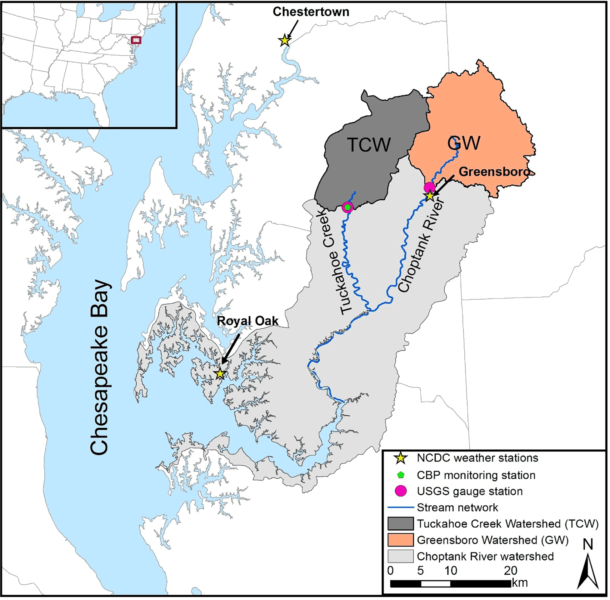
Figure 1 The location of the Tuckahoe Creek Watershed (left) and Greensboro Watershed (right) (adapted from Lee et al., 2016a).

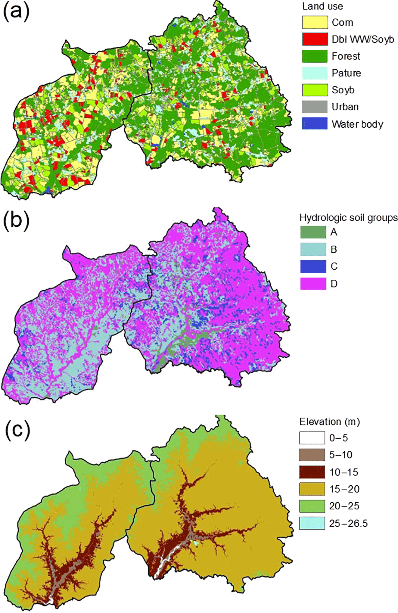
Figure 2 The physical characteristics of the Tuckahoe Creek Watershed (left) and Greensboro Watershed (right); (a) land use, (b) hydrologic soil groups, and (c) elevation (adapted from Lee et al., 2016a). Note: Dbl WW/Soyb stands for double crops of winter wheat and soybean in a year. Hydrologic soil groups (HSGs) are characterized as follows: Type A – well-drained soils with a 7.6–11.4 mm h⁻¹ water infiltration rate; Type B – moderately well-drained soils with 3.8–7.6 mm h⁻¹; Type C – moderately poorly drained soils with 1.3–3.8 mm h⁻¹; Type D – poorly drained soils with 0–1.3 mm h⁻¹ (Netisch et al., 2011).

Table 1 Soil properties and land use distribution of the Tuckahoe Creek Watershed (TCW) and Greensboro Watershed (GW) (adapted from Lee et al., 2016a).

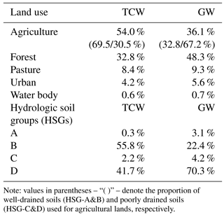
Note: values in parentheses – “( )” – denote the proportion of well-drained soils (HSG-A&B) and poorly drained soils (HSG-C&D) used for agricultural lands, respectively.

2.2 SWAT

The SWAT is a process-based watershed model, developed to assess the impact of human activities and land use on water and nutrient cycles within agricultural watersheds (Neitsch et al., 2011). The SWAT divides a watershed into sub-watersheds using a digital elevation model (DEM), and each sub-watershed is further divided into hydrologic response units (HRUs) based on a unique combination of land use, soil type, and slope. Model simulation is performed at the HRU level, and the simulated outputs aggregated at the sub-watershed and then further at the watershed level through routing processes. The amounts of surface runoff and infiltration are calculated based on the Soil Conservation Service (SCS) curve number (CN) method, and the CN values are updated daily based on soil permeability, land use type, and antecedent soil water conditions. Water infiltrated into soils is either delivered to streams through lateral flow or further percolated into groundwater, when soil water content exceeds field capacity. The groundwater portion is then transported to streams through groundwater flow, percolated into the deep groundwater aquifer, or discharged to the soil profile. The amount of nitrate in soils is increased by nitrification, mineralization of soil organic and crop residue, biological N fixation, and fertilization, and decreased through denitrification and plant uptake (Neitsch et al., 2011). Nitrate fluxes move via surface runoff, lateral flow, percolated water from soil to groundwater, and groundwater flow. Nitrate concentration in the mobile water (i.e., surface runoff, lateral flow, and percolated water) is first determined and then nitrate fluxes in the mobile water are calculated based on the nitrate concentration and the amount of mobile water. Nitrate in groundwater is re-distributed in four ways: remains in the groundwater, recharges to deep groundwater, moves to streams, or discharges to the soils. Nitrate removal by biological and chemical processes in groundwater is simulated by the first-order kinetics. Refer to Netisch et al. (2011) for further details.

The SWAT model has the capability of simulating the impacts of CO₂ concentration on ET and biomass accumulations. The Penman–Monteith method used for this study considers CO₂ effects on ET based on the relationship between plant stomatal conductance and CO₂ concentration:

$$\begin{array}{}\text{(1)}& g_{\mathrm{l},{\mathrm{CO}}_{\mathrm{2}}}=g_{\mathrm{l}}\times [\mathrm{1.4}-\mathrm{0.4}\times ({\mathrm{CO}}_{\mathrm{2}}/\mathrm{330}\left)\right],\end{array}$$

where $g_{\mathrm{l},{\mathrm{CO}}_{\mathrm{2}}}$ is the leaf conductance modified to reflect CO₂ effects, and g_l is the leaf conductance without the effect of CO₂. The equation shows the linear reduction of the leaf conductance with increasing CO₂ and results in a 40 % reduction in leaf conductance for all plants when CO₂ concentration is doubled. According to Eq. (1) elevated CO₂ concentrations decrease plant stomatal conductance and canopy resistance, subsequently reducing ET. Refer to Neitsch et al. (2011) for details on the Penman–Monteith method.

The simulation of crop growth in the SWAT is based on potential heat unit theory. The model considers the impacts of CO₂ concentration on crop biomass growth by modifying the radiation-use efficiency (RUE) of the plant as follows:

$$\begin{array}{}\text{(2)}& \mathrm{RUE}={\displaystyle \frac{\mathrm{100}\cdot {\mathrm{CO}}_{\mathrm{2}}}{{\mathrm{CO}}_{\mathrm{2}}+\exp (r_{\mathrm{1}}-r_{\mathrm{2}}\cdot {\mathrm{CO}}_{\mathrm{2}})}},\end{array}$$

where RUE is the radiation-use efficiency of a plant, and r₁and r₂ are coefficients.

$$\begin{array}{}\text{(3)}& \mathrm{\Delta }\mathrm{bio}=\mathrm{RUE}\cdot H_{\mathrm{phosyn}},\end{array}$$

where Δbio is a potential increase in plant biomass on a given day and H_phosyn is the amount of intercepted photosynthetically active radiation on a given day.

2.3 Baseline SWAT input data

Climate and geospatial data needed for the SWAT simulation are summarized in Table 2. Daily precipitation and temperature were obtained from three meteorological stations operated by the National Oceanic and Atmospheric Administration (NOAA) National Climate Data Center (NCDC) at Chestertown, Royal Oak, and Greensboro, Maryland (USC00181750, USC00187806, and US1MDCL0009, respectively). Due to data unavailability, humidity, wind speed, and solar radiation were generated using the SWAT built-in weather generator (Neitsch et al., 2011). Monthly streamflow data were downloaded from US Geological Survey (USGS) gauge stations on Tuckahoe Creek near Ruthsburg (USGS no. 01491500) and the Choptank River near Greensboro (USGS no. 01491000) (Fig. 1). The USGS LOAD ESTimator (LOADEST, Runkel et al., 2004) was used to generate continuous monthly nitrate loads from nitrate grab sample data (133 samples over the simulation period) that were obtained from the Chesapeake Bay Program (CBP, TUK no. 0181) for the TCW and from USGS gauge station data (USGS no. 01491000) for the GW. The LOADEST is commonly used to generate continuous data from discrete data, and it has been shown to accurately generate water quality variables (Jha and Jha, 2013; Lee et al., 2016b). The land use, soil maps, and DEM were prepared as shown in Table 2.

Table 2 List of the SWAT model input data.

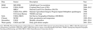
Note: MD-DNR: Maryland Department of Natural Resources, USDA-NASS: USDA-National Agricultural Statistics Service, MRLC: Multi-Resolution Land Characteristics Consortium, USDA-FSA-APFO: USDA-Farm Service Agency-Aerial Photography Field Office, TIGER: Topologically Integrated Geographic Encoding and Referencing, and USDA-NRCS: USDA-Natural Resources Conservation Service.

We identified representative agricultural practices for this region using multiple geospatial data (Lee et al., 2016a). Major crop rotations and their year-to-year placement were derived through analysis of the USDA-National Agricultural Statistics Service (NASS) Cropland Data Layer (CDL) for the period of 2008–2012. We assumed that crop rotation and land use did not change over the simulation period so that agricultural N input did not vary for the baseline and GCM scenarios. Detailed agricultural management information (e.g., the amount, type, and application timing of fertilizer, and planting and harvesting timings of individual crops) was developed through literature review and communications with local experts (Table A1). Detailed information about the development of crop rotation and land management is available in Lee et al. (2016a).

2.4 Baseline SWAT calibration and validation

The SWAT model simulations were performed at a monthly time step for 16 years; this included 2-year warm-up (1999–2000), 8-year calibration (2001–2008), and 6-year validation (2009–2014) periods. The SWAT model was run at a daily time step based on daily climate input data, and daily outputs were aggregated to monthly outputs. It should be noted that due to unavailability of water quality observations prior to 2001, model calibration and validation were initiated from 2001. Compared to past 30-year precipitation data (1981–2010), the climate condition over the calibration period (2001–2008) was shown to include representative wet, dry, and average climate conditions, while the validation period (2009–2014) was dominated by wet conditions. Critical parameters used for model calibration were selected based on previous studies conducted in this region (Sexton et al., 2010; Yeo et al., 2014; Lee et al., 2016a) and allowable ranges of these parameters were derived from the literature as indicated in Table 3. Streamflow parameters were manually calibrated and then nitrate parameters were adjusted following SWAT calibration guidelines (Arnold et al., 2012). A set of parameters that produced the best model performances and fulfilled model performance criteria suggested by Moriasi et al. (2007) were chosen for model validation. Model performance was evaluated using the following statistics: Nash–Sutcliffe efficiency coefficient (NSE), root mean square error (RMSE) standard deviation (SD) ratio (RSR), and percent bias (P-bias).

$$\begin{array}{}\text{(4)}& {\displaystyle }& {\displaystyle }\mathrm{NSE}=\mathrm{1}-\left[{\displaystyle \frac{\sum _{i=\mathrm{1}}^n(O_i-S_i{)}^{\mathrm{2}}}{\sum _{i=\mathrm{1}}^n(O_i-\stackrel{\mathrm{‾}}{O}{)}^{\mathrm{2}}}}\right],\text{(5)}& {\displaystyle }& {\displaystyle }\mathrm{RSR}={\displaystyle \frac{\mathrm{RMSE}}{{\mathrm{SD}}_{\mathrm{obs}}}}={\displaystyle \frac{\left[\sqrt{\sum _{i=\mathrm{1}}^n(O_i-S_i{)}^{\mathrm{2}}}\right]}{\left[\sqrt{\sum _{i=\mathrm{1}}^n(O_i-\stackrel{\mathrm{‾}}{O}{)}^{\mathrm{2}}}\right]}},\text{(6)}& {\displaystyle }& {\displaystyle }P\text{-bias}=\left[{\displaystyle \frac{\sum _{i=\mathrm{1}}^n(O_i-S_i)\times \mathrm{100}}{\sum _{i=\mathrm{1}}^n{O}_i}}\right],\end{array}$$

where O_i is the observed data at time step i, S_i is the simulated output at time step i, $\stackrel{\mathrm{‾}}{O}$ is the mean of observed data over all time steps, and n is the total number of observed data. We also calculated NSE for the natural logarithm of streamflow to evaluate model performance for low flows (Kiptala et al., 2014). In addition, the 95 % prediction uncertainty (95 PPU) band was represented to evaluate model uncertainty (Singh et al., 2014). The 95 PPU was computed based on all simulated outputs generated during the calibration process. The 95 PPU was represented as the range of values between the 2.5 and 97.5 percentiles of the cumulative distribution of simulated outputs.

Table 3 List of calibrated parameters.

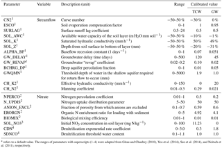
^* refers to a default value. The ranges of parameters with superscripts (1–4) were adapted from Gitau and Chaubey (2010), Yeo et al. (2014), Seo et al. (2014), and Neitsch et al. (2011), respectively.

2.5 Climate sensitivity and GCM scenarios

To evaluate the impacts of climate variability and change on watershed hydrological processes, climate sensitivity and GCM scenarios were prepared as illustrated below (see Sect. 2.5.1 and 2.5.2). The calibrated SWAT model was simulated using the climate sensitivity and GCM scenarios for comparison with baseline water and nitrate budgets.

2.5.1 Climate sensitivity scenarios

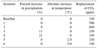
A climate sensitivity analysis aids in identifying the degree or threshold of responses of hydrologic variables to climate-induced modifications, and a sensitivity scenario generally assumes constant changes throughout the year (Mearns, 2001). Following the approach in Mearns (2001), six climate sensitivity scenarios were prepared by modifying the baseline data (1999–2014) to assess individual effects of elevated CO₂ concentrations, precipitation, and temperature on watershed hydrological processes (Table 4). Sensitivity scenarios were designed to change one variable while holding other variables constant throughout the simulations. Baseline precipitation and temperature were modified by percent and absolute changes using anomaly and absolute data, respectively, as illustrated in Najjar et al. (2009). They reported mean temperature and precipitation changes over CB for three future periods (2010–2039, 2040–2069, and 2070–2099) relative to the baseline period (1971–2000) based on GCM outputs (Najjar et al., 2009). We used the maximum increase rate (and value) for 2040–2069 (precipitation: 11 % and temperature: 2.9 ^∘C) and 2070–2099 (precipitation: 21 % and temperature: 5.0 ^∘C) to set the precipitation and temperature sensitivity scenarios. For example, baseline precipitation increased by 11 and 21 % for Scenarios 3 and 4, respectively, and 2.9 and 5.0 ^∘C were added to the baseline temperature for Scenarios 5 and 6, respectively (Table 4). The baseline CO₂ concentration was set as the default value (330 ppm) for simulations. For the first and second scenarios, the baseline CO₂ concentration was replaced with 590 and 850 ppm, respectively. The upper value of 850 ppm was used because GCMs used for temperature and precipitation sensitivity scenarios were forced with the assumption of CO₂ concentration of 850 ppm (Najjar et al., 2009). The lower value of 590 ppm (the average of 330 and 850 ppm) was considered to be the level of CO₂ concentration around the middle of the 21st century.

Table 4 Climate sensitivity scenarios developed by modifying baseline values.

2.5.2 GCM scenario

A GCM-based scenario is the most commonly used method for assessing future climate change impacts (Mearns, 2001). We downloaded projected climate data (e.g., daily precipitation and maximum and minimum temperature) from the World Climate Research Program's (WCRP's) Coupled Model Intercomparison Project5 (CMIP5) archive (Brekke et al., 2013). Five GCM data under the Representative Concentration Pathway (RCP) 8.5 scenario were downloaded (Table A2), because the RCP 8.5 indicates the highest value of CO₂ concentration in the CMIP5. To be consistent with the period of the baseline data (1999–2014), 16-year future data (2083–2098) were used in this study. We further refined GCM data using the delta change method because spatially downscaled data are consistent with historical observations at the global scale, but could be significantly inconsistent at fine spatial scales, such as a watershed (Wang et al., 2014). The delta change method was calculated as follows:

$$\begin{array}{}\text{(7)}& {\displaystyle }& {\displaystyle }{P}_{\mathrm{delta}}={\mathrm{GCM}}_{P\text{-future},\mathrm{monthly}}/{\mathrm{GCM}}_{P\text{-baseline},\mathrm{monthly}},\text{(8)}& {\displaystyle }& {\displaystyle }{T}_{\mathrm{delta}}={\mathrm{GCM}}_{T\text{-future},\mathrm{monthly}}-{\mathrm{GCM}}_{T\text{-baseline},\mathrm{monthly}},\text{(9)}& {\displaystyle }& {\displaystyle }{\mathrm{DGCM}}_{P\text{-future},\mathrm{daily}}={\mathrm{OBS}}_{P\text{-baseline},\mathrm{daily}}\times P_{\mathrm{delta}},\text{(10)}& {\displaystyle }& {\displaystyle }{\mathrm{DGCM}}_{T\text{-future},\mathrm{daily}}={\mathrm{OBS}}_{T\text{-baseline},\mathrm{daily}}+T_{\mathrm{delta}},\end{array}$$

where P_delta and T_delta indicate precipitation (P) and temperature (T) biases in GCM data, respectively, GCM_{future,monthly} and GCM_{baseline,monthly} indicate the monthly average of GCM data for the future (2083–2098) and baseline (1999–2014) periods, respectively, OBS_{baseline,daily} indicates observed daily climate, and DGCM_future,daily indicates unbiased future climate data. We calculated the ensemble mean of delta-change values from the five GCMs, because substantial variations existed among the GCM projections (Shrestha et al., 2012; Van Liew et al., 2012). Then, the SWAT model was simulated using the ensemble mean to predict hydrological processes under future climate conditions. Similar to the baseline scenario, humidity, wind speed, and solar radiation values were generated using the SWAT built-in weather generator owing to data unavailability. We assumed the CO₂ concentration for the GCM scenario to be 936 ppm, as the specified CO₂ concentration under the RCP8.5 scenario (Meinshausen et al., 2011).

2.6 Analyses of simulation outputs

Simulated outputs were summarized at multiple temporal scales (e.g., monthly, seasonal, and annual). Annual averages of streamflow, ET, and nitrate loads were calculated to investigate changes in water and nitrate budgets in response to climate sensitivity and GCM scenarios. The response of crop growth to climate variability and change was also analyzed to show the effects of modified crop biomass on hydrology and the N cycle. For comparative analyses between two watersheds, water and nitrate yields were summarized seasonally for climate sensitivity scenarios (i.e., summer (April–September) and winter (October–March)) and monthly for the GCM scenario. Note that water and nitrate yields indicate the summations of water and nitrate fluxes transported from lands to streams by surface runoff, lateral flow, and groundwater flow. All simulation outputs were normalized by total watershed size.

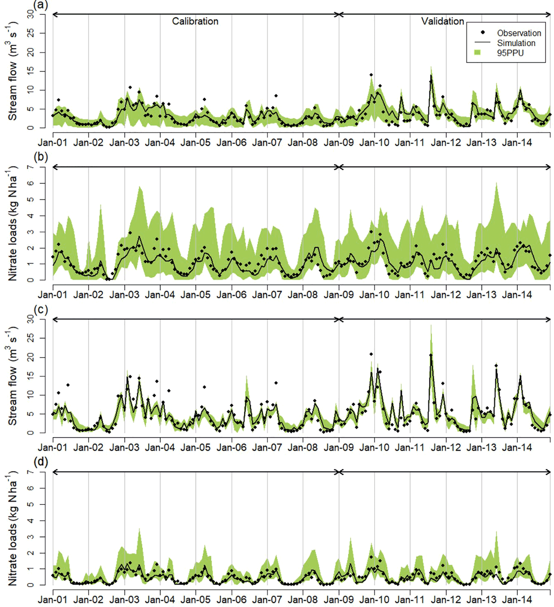
Figure 3 Simulated and observed monthly streamflow and nitrate loads for the (a, b) TCW and (c, d) GW during calibration and validation periods. Note: 95 PPU stands for 95 % prediction uncertainty.

We conducted a statistical analysis to test whether the simulation results under climate sensitivity and GCM scenarios were statistically different from those under the baseline scenario using parametric (paired t-test) and nonparametric (Wilcoxon signed rank) methods. Note that we used monthly outputs (168 samples over 14 years) for this analysis. The statistical significance for the difference was indicated by the p-value.

3 Results and discussions

3.1 Model calibration and validation

Monthly simulations for streamflow and nitrate loads were compared with corresponding observations (Fig. 3). Results show that simulated values for monthly streamflow were in good agreement with observations, but simulated peak streamflows were underestimated relative to observations. This underestimation was attributed to the inherent limitations of the SWAT model and limited climate data to capture local storm effects as it does not account for the intensity and duration of the precipitation (Qiu et al., 2012). Previous studies conducted in this region showed similar results, though the overall simulation results accurately replicated the observations (Yeo et al., 2014; Lee et al., 2016a). Simulated nitrate loads were also well matched with actual observations and the uncertainty band (shown as green in Fig. 3) captured most observations in the two watersheds. Overall, model performance measures fulfilled “good” (e.g., 0.65 < NSE ≤ 0.75) or “very good” (0.75 < NSE) criteria for streamflow and at least “satisfactory” (0.5 < NSE ≤ 0.65) for nitrate loads (Table 5). The model performance measures for low flows (NSE for the natural logarithm of streamflow) also indicated “satisfactory” to “very good” (Table 5). These results demonstrated that the calibrated model replicated actual conditions reasonably well (Moriasi et al., 2007; Arnold et al., 2012).

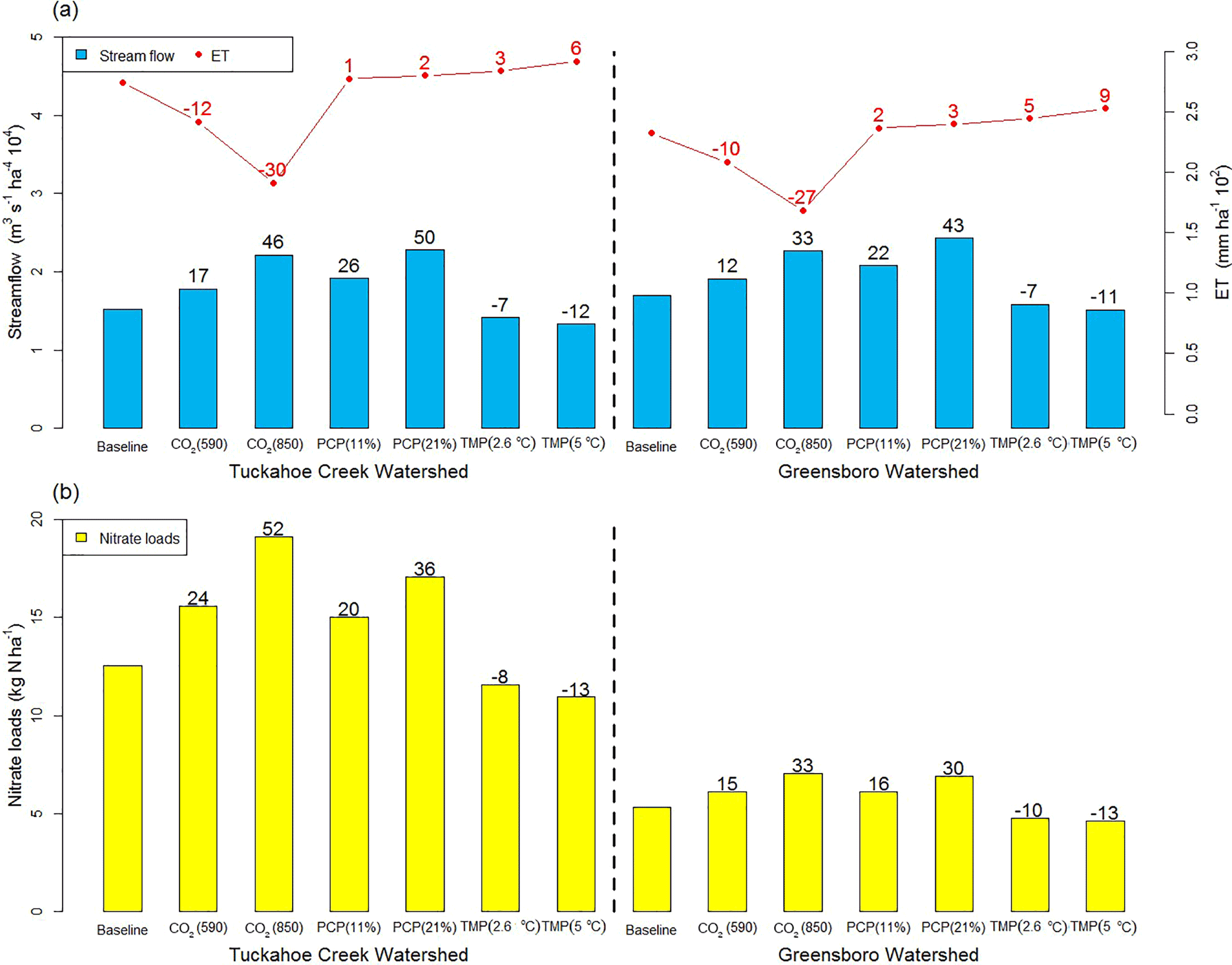
Figure 4 The 14-year average of annual hydrologic variables under the baseline and climate sensitivity scenarios at the watershed scale: (a) streamflow and evapotranspiration (ET), and (b) nitrate loads. Note: the red and black numerical values above the bar and dot graphs, respectively, indicate the relative changes (%) in hydrologic variables for climate sensitivity scenarios relative to the baseline scenario (relative change (%) = (sensitivity scenarios − baseline) ∕ baseline × 100). PCP and TMP stand for precipitation and temperature, respectively.

Table 5 Model performance measures for monthly streamflow and nitrate loads.

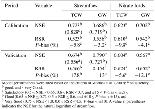
Model performances were rated based on the criteria of Moriasi et al. (2007): ^a satisfactory, ^b good, and ^c very Good.
^a Satisfactory (0.5 < NSE ≤ 0.65, 0.6 < RSR ≤ 0.7, and ±15 ≤ P-bias < ±25),
^b Good (0.65 < NSE ≤ 0.75, 0.5 < RSR ≤ 0.6, and ±10 ≤ P-bias < ±15), and
^c Very Good (0.75 < NSE ≤ 1.0, 0.0 < RSR ≤ 0.5, P-bias < ±10). A value in parentheses indicates the NSE for the natural logarithm of streamflow.

3.2 Responses to climate sensitivity scenarios

3.2.1 Water and nitrate budgets

The 14-year averages of annual hydrologic variables under the baseline and climate sensitivity scenarios are presented in Fig. 4. Elevated CO₂ concentrations (590 and 850 ppm) and precipitation increases (11 and 21 %) led to significant increases in annual streamflow and nitrate loads by 50 and 52 % for the TCW and 43 and 33 % for the GW, respectively, relative to the baseline scenario (p-value < 0.01) (Fig. 4). Elevated CO₂ concentrations lowered plant stomatal conductance, resulting in a decrease in ET of 30 % and thereby increased streamflow and corresponding increases in nitrate loads (Fig. 4). The reduced rate of ET (driven by CO₂ concentrations of 850 ppm) demonstrated in this study is supported by previous studies using SWAT, such as Ficklin et al. (2009, −40 %; 970 ppm) and Pervez et al. (2015, −12 %; 660 ppm). Precipitation increase resulted in a direct increase in streamflow, leading to increased nitrate loads. Compared to the baseline scenario, a temperature increase of 5 ^∘C significantly reduced annual streamflow and nitrate loads by 12 and 13 % for the TCW and 11 and 13 % for the GW (p-value < 0.01), respectively, due to intensified ET (Fig. 4).

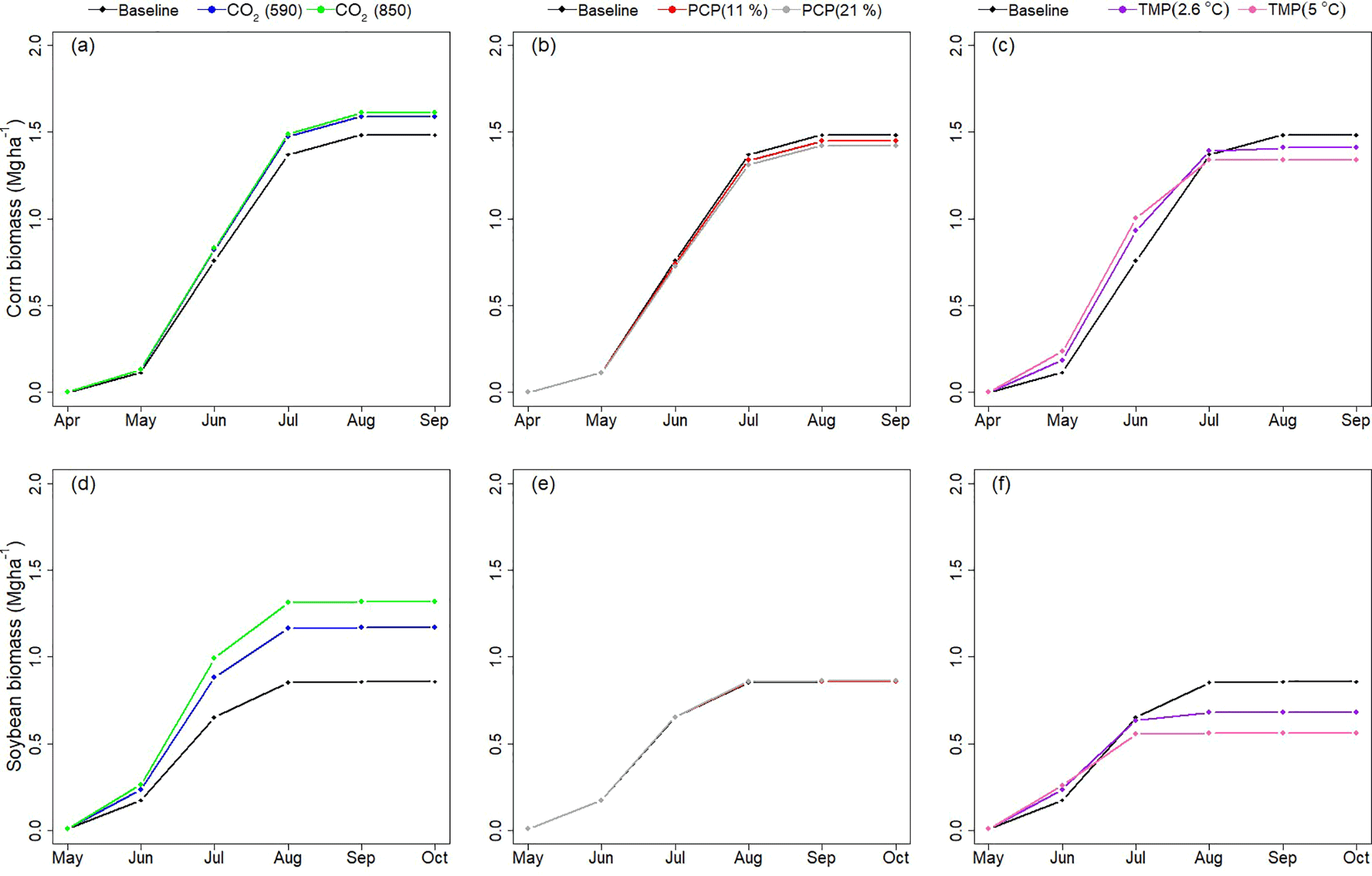
Figure 5 The responses of crop biomass growth to the climate sensitivity scenario: (a–c) corn and (d–f) soybean. Note: PCP and TMP in the legend stand for precipitation and temperature, respectively.

It should be noted that the standard version of SWAT tends to overestimate the impact of CO₂ on reduction of ET (Eckhardt and Ulbrich, 2003). Maximum leaf area index (LAI) is assumed to be constant regardless of variation in CO₂ concentration in SWAT. However, maximum LAI is known to increase with increasing CO₂ concentration (Eckhardt and Ulbrich, 2003). In addition, the degree of reduction in stomatal conductance varies by plant species, which also is not taken into account in the SWAT model. Another model simplification, which increases uncertainty, is the application of the same reduction rate to all plants. For example, C3 crops (soybean and wheat) are known to have less reduction in stomatal conductance with rising CO₂ concentration compared to C4 crops (corn) (Ainsworth and Rogers, 2007). Both factors could contribute to overestimating reduction of ET and resultant increase in streamflow and nitrate loads (Eckhardt and Ulbrich, 2003).

Changes in crop growth under climate sensitivity scenarios had great impacts on water and nitrate budgets. Although precipitation increase resulted in the greatest increase in annual streamflow, annual nitrate loads were greater under elevated CO₂ concentrations (Fig. 4), due to increased crop biomass and high N availability from mineralization of crop residues (Fig. 5a, b). Elevated CO₂ concentrations stimulated crop growth by decreasing water demand and increasing radiation-use efficiency (Abler and Shortle, 2000; Parry et al., 2004). For example, simulated corn and soybean biomass increased from 1.5 and 0.9 Mg ha⁻¹ (baseline concentration of 330 ppm) to 1.6 and 1.3 (CO₂ concentration of 850 ppm) Mg ha⁻¹, respectively (Fig. 5a, b). Increased crop biomass left greater amounts of crop residue following crop harvest (winter seasons: October–March), which contributed to increasing nitrate in soils through mineralization (Lee et al., 2016a). Our simulation results indicated that mineralized nitrate under elevated CO₂ concentrations increased by 27 % for the TCW and 23 % for the GW during winter seasons, compared to the baseline values (Fig. A1). Increased crop residue resulted in greater nitrate loads under elevated CO₂ concentrations than under conditions of increased precipitation. In contrast, temperature increase led to lower crop biomass than the baseline value, due to increased heat stress (Fig. 5c, f). Lower biomass reduced remaining crop residue and subsequently reduced mineralized nitrate by 22 % during winter seasons, compared to the baseline value (Fig. A1). Reduction of mineralized nitrate contributed to decreased nitrate loads in conjunction with intensified ET. Precipitation increase slightly decreased corn biomass because increased precipitation reduced the availability of nutrients for crops (Fig. 5b), leading to increased nutrient stress. However, soybean biomass did not change in response to precipitation increase (Fig. 5e) since soybean crops can generate N through fixation as needed.

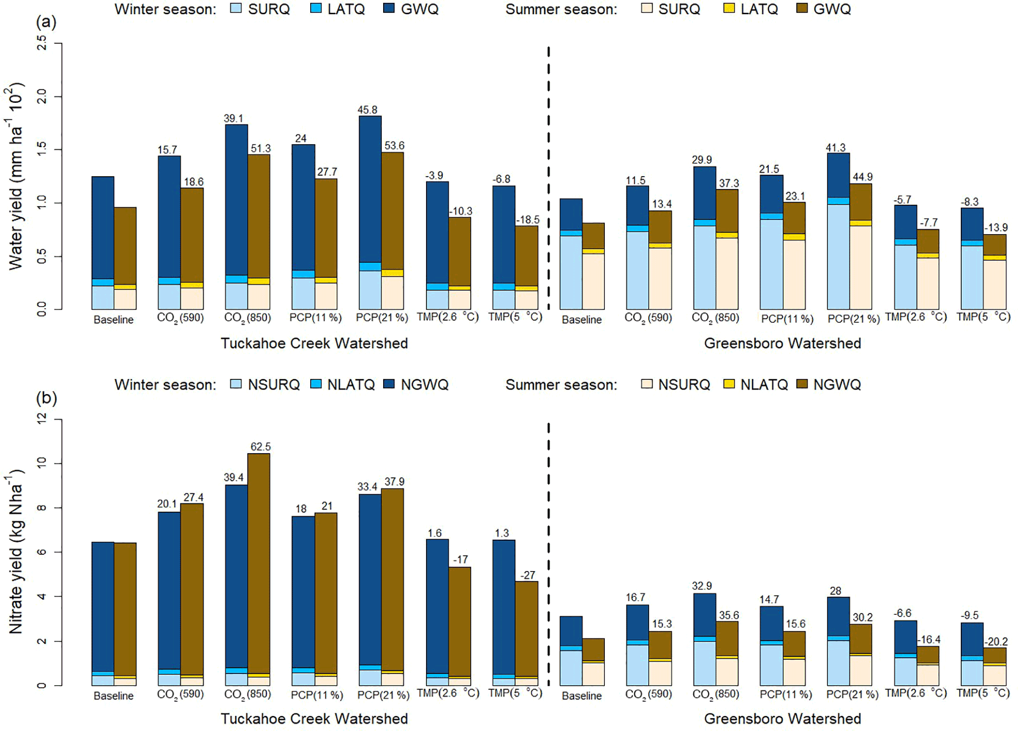
Figure 6 The 14-year average of seasonal hydrologic variables under the baseline and climate sensitivity scenarios at the watershed scale: (a) water and (b) nitrate yields. Note: the number on the bar graph indicates the relative changes (%) in hydrologic variables for climate sensitivity scenarios relative to the baseline scenario. Water and nitrate yields indicate the summations of water and nitrate fluxes transported from lands to streams by surface runoff, lateral flow, and groundwater flow. PCP and TMP stand for precipitation and temperature, respectively. SURQ, LATQ, and GWQ indicate water fluxes transported by surface runoff, lateral flow, and groundwater flow, respectively. NSURQ, NLATQ, and NGWQ indicate nitrate fluxes transported by surface runoff, lateral flow, and groundwater flow, respectively.

3.2.2 Comparative analyses

For the purpose of comparing the two watersheds in response to climate sensitivity scenarios, 14-year averages of seasonal water and nitrate yields were calculated (Fig. 6). Both elevated CO₂ concentrations and precipitation increase led to greater water and nitrate yields for the two watersheds during winter and summer seasons, compared to the baseline scenario. However, the seasonal pattern of nitrate yield differed between the two watersheds. Wintertime water yield was greater than summertime water yield for both watersheds, which was consistent with the seasonal pattern of nitrate yield for the GW. However, summertime nitrate yield increases were greater than wintertime increases for the TCW, apparently due to the difference in percent agricultural lands between the TCW (54.0 %) and GW (36.1 %). Increased water yield could accelerate the export of nitrate added to the watersheds through fertilizer activities, which mainly occurs during summer seasons. Accordingly, increased water yield caused by elevated CO₂ concentrations and precipitation increase induced considerable increase in summertime nitrate yield by ∼ 62.5 % for the TCW, while only moderately increasing yield by ∼ 35.6 % for the GW, which is dominated by forest instead of croplands.

Temperature increase reduced summertime water and nitrate yields by 18.5 and 27 % for the TCW and 13.9 and 20.2 % for the GW, respectively, mainly due to increased water loss by ET (Table A3). Wintertime water yield also decreased for the two watersheds, but changes in wintertime nitrate yield differed between the two watersheds. A decrease of 9.5 % in wintertime nitrate yield was found for GW, but wintertime nitrate yield increased by 1.6 % for the TCW (Fig. 6b), due to modified crop growth patterns and contrasting soil characteristics between the two watersheds. Temperature increase can drive crops to reach maturity earlier while exerting increased heat stress on crops, leading to lower biomass compared to the baseline (Fig. 5c, f). These two factors collectively reduced soil water and nitrate consumption by crops at the end of the growth stage under temperature increase scenarios, subsequently increasing soil water content and nitrate leaching compared to the baseline (Fig. A2). Nitrate leached into groundwater was discharged to streams through groundwater flow during winter seasons. The TCW showed increased nitrate leaching of 1.0 kg N ha⁻¹ compared to the GW, due to a larger percentage of well-drained soils with a high infiltration rate. Different leaching rates between the TCW and GW soils led to a greater increase in wintertime nitrate flux transported by groundwater flow (NGWQ) for the TCW (0.21 kg N ha⁻¹) compared to the GW (0.16 kg N ha⁻¹) (Fig. 6b). However, intensified ET reduced wintertime water and nitrate fluxes transported by surface runoff (SURQ and NSURQ, respectively) for the two watersheds (Table A3), while water fluxes transported by lateral and groundwater flow (LATQ and GWQ, respectively) were rarely changed. Because the majority of water flux was transported by groundwater flow for the TCW and surface runoff for the GW (Fig. 6a), a decrease in SURQ led to a substantial reduction of wintertime NSURQ for GW (0.45 kg N ha⁻¹) with less reduction shown in the TCW (0.12 kg N ha⁻¹), compared to the baseline (Fig. 6b). Therefore, both increased NGWQ and decreased NSURQ during winter seasons collectively led to an increasing pattern of wintertime nitrate yield for the TCW and a decreasing pattern for the GW, compared to the baseline scenario. Note that denitrification was rarely affected by temperature increase because reduced soil water content resulting from increased ET at higher temperatures decreased denitrification.

3.3 Responses to the GCM scenario

3.3.1 Comparison of climate data

The monthly averages of mean temperature and cumulative precipitation under the baseline scenario were compared with the ensemble means of five GCMs (Fig. 7). Projected temperature was constantly higher than the baseline value throughout the year by 3.8–6.2 ^∘C (Fig. 7a). Compared to the baseline, projected precipitation was greater except for May and October (Fig. 7b). Monthly cumulative precipitation was up to 19 mm greater in August and up to 11 mm lower in October, in comparison to the baseline values. Note that the annual average of mean temperature increased from 13.9 ^∘C (baseline) to 18.6 ^∘C (projection), and the annual average of cumulative precipitation also increased from 1221 mm (baseline) to 1322 mm (projection).

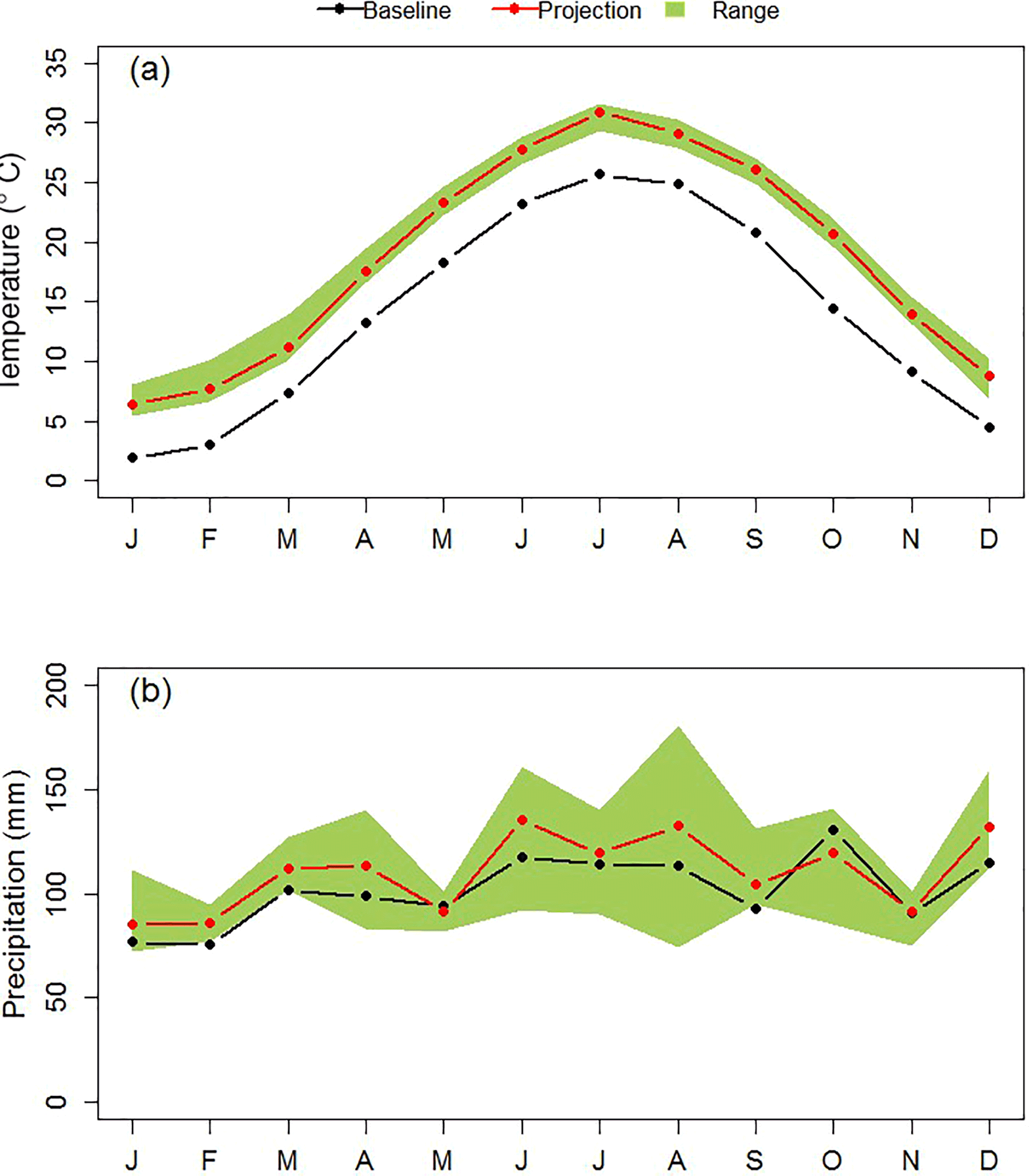
Figure 7 Monthly average of (a) mean temperature and (b) cumulative precipitation for the baseline (2001–2014) and future (2085–2098) periods. Note: “Projection” stands for the ensemble mean of five GCM data, and the range stands for the interval between the maximum and minimum values of five GCM data.

3.3.2 Water and nitrate budgets

Baseline hydrologic variables (e.g., streamflow, ET, and nitrate loads) are compared with the simulated outputs in Table 6. Relative to the baseline scenario, annual streamflow and nitrate loads significantly increased by 70 and 66 % for the TCW and 50 and 56 % for the GW, respectively (p-value < 0.01). These increasing patterns were mainly caused by two factors: (1) increased precipitation and (2) decreased ET resulting from an elevated CO₂ concentration of 936 ppm. Annual precipitation increased by 8 % and elevated CO₂ concentrations reduced ET by 32 % for the TCW and 26 % for the GW (Table 6).

Table 6 The 14-year average of hydrologic variables under the baseline and GCM scenarios.

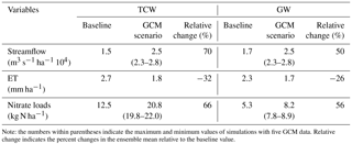
Note: the numbers within parentheses indicate the maximum and minimum values of simulations with five GCM data. Relative change indicates the percent changes in the ensemble mean relative to the baseline value.

3.3.3 Comparative analyses

Responses of the two watersheds to the GCM scenario were compared using the monthly averages of water and nitrate yields as shown in Fig. 8. Relative to the baseline, projected water and nitrate yield was greater over the year. The greatest increase in water yield was observed in August and September when the increased rate of precipitation was greatest. However, the increased rate of nitrate yield was higher in April than other months, due to a significant export of nitrate from fertilizer applications.

The increased rate of nitrate yield (under the GCM scenario relative to the baseline scenario) was 5.2 kg N ha⁻¹ greater overall in the TCW compared to the GW, mainly due to the difference in watershed characteristics (Fig. 8b, d). First, a larger percentage of croplands in TCW led to greater nitrate export from fertilizer application compared to GW with a smaller percent of croplands. This was because increased water yield resulting from an elevated CO₂ concentrations and increased precipitation promoted the export of nitrate in the soil profile (Suddick et al., 2013). For example, nitrate yield increased by 1.4 kg N ha⁻¹ for the TCW and 0.9 kg N ha⁻¹ for the GW in April, when fertilizer application occurred, compared to the baseline. Second, a larger percentage of poorly drained soils in the GW contributed to reducing nitrate yield via greater potential of denitrification, compared to the TCW dominated by well-drained soils, under the GCM scenario. Increased soil water content resulting from an elevated CO₂ concentration of 936 ppm provided anaerobic conditions for denitrification. Compared to the baseline, the GW and TCW showed increased nitrate removal by denitrification of 3.9 and 0.5 kg N ha⁻¹ under the GCM scenario, respectively. Eventually, the GW lost 8.7 kg N ha⁻¹ more nitrate via denitrification than the TCW, which likely led to a lower nitrate yield for the GW.

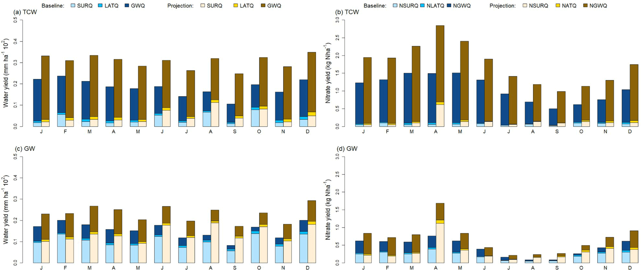
Figure 8 The 14-year average of monthly water and nitrate yields under the baseline and GCM scenarios. Note: the descriptions of abbreviations are available in the caption of Fig. 6.

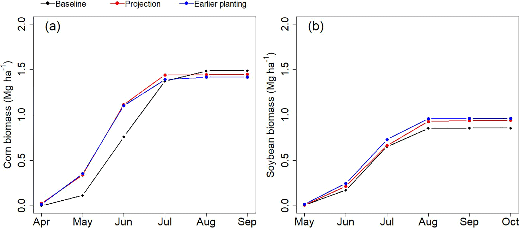
Figure 9 Crop biomass growth under the baseline and GCM scenarios: (a) corn and (b) soybean. Note: “Projection” stands for the simulated biomass planted on the original planting dates under the GCM scenario. Earlier planting indicates the simulated biomass planted 10 days earlier than the original planting dates under the GCM scenario.

4 Implications and limitations

The key results of this study suggest important future research for improving our understanding of climate change impacts on nutrient loads into the CBW. Analysis of climate variability and change impacts on watershed hydrological processes illustrate the close relationship between agricultural activities and future nitrate export in the watershed dominated by croplands, due to excessive export of nitrate from springtime fertilizer application. Changes in crop growth resulting from climate change are likely to alter agricultural activities and associated nitrate loads. Fertilizer application might increase in the future because increased extreme climate conditions (e.g., high-intensity rainfall and flooding) might lead to increased risk of nutrient loss to leaching and runoff, reducing the fertilizer use efficiency of field crops (Suddick et al., 2013). Our simulation indicated considerable increases in nitrate transported by surface runoff (NSURQ) due to increased precipitation in April, when the vast majority of fertilizers were applied (Fig. 8b, d). As a result, projected corn biomass appeared to be 0.03 Mg ha⁻¹ lower than the baseline value, likely due to increased nutrient stress (Fig. 9a). Conversely, soybean biomass increased under the GCM scenario because soybean could accumulate N through biological fixation and elevated CO₂ concentrations contributed to biomass growth (Fig. 9b). To adapt to warmer temperatures, early planting of summer crops could be suggested to increase crop production while reducing heat stress (Woznicki et al., 2015). For example, when planting dates were shifted 10 days earlier, soybean yield increased on average by 0.03 Mg ha⁻¹ (Fig. 9b). Contrary to our expectation, corn yield decreased under the earlier planting date, due to increased nutrient stress resulting from intensified precipitation. Lastly, irrigation patterns could be changed due to decreased ET resulting from elevated CO₂ concentrations. However, there are limited studies investigating projected future agricultural practices. Therefore, it is crucial to investigate potential agricultural activities under climate change scenarios and their projected effects on nitrate loads.

Climate change-driven modifications indicated a potential overall increase in nitrate export. Therefore, the importance of conservation practices aimed at N mitigation would be even more critical in the future. Comparative analyses of two watersheds can provide a practical guideline and have implications for agricultural watersheds in coastal areas in the CBW because our analyses considered climate change impacts on croplands (crop growth, water and nutrient cycling) and nutrient transport mechanisms in the context of detailed agricultural management practices. In addition, the two watersheds showed the typical site characteristics in the coastal watershed, in terms of topographic and soil characteristics, and the agricultural practices commonly used in the southern CBW. Hence, the findings from this study can be applicable to other catchments in the CBW region in preparing climate change adaptation strategies. For example, the effective management of nutrients applied in manure or fertilizer would be even more critical for reducing nitrate export from a watershed dominated by croplands. Winter cover crops, which are widely implemented in this region, would likely show increased value in mitigating agricultural nitrate loss during winter seasons, considering increased N availability and increased wintertime precipitation. In a watershed dominated by poorly drained soils, wetland restoration would be well positioned to enhance denitrification (McCarty et al., 2014), as would be the use of drainage control structures on ditches and tiles draining prior converted croplands (poorly drained areas of the farm landscape).

Note that although forest litterfall can have a significant impact on nutrient cycles (Zhang et al., 2014), the current version of the SWAT model is limited in representing forest impacts (Yang et al., 2016). In our simulation, growth of deciduous trees was simulated for forest areas with the default setting. This setting allowed tree growth to affect water and nutrient cycling via ET and uptake, but simulated tree growth was considerably underestimated compared to actual growth and litterfall was rarely considered (Yang et al., 2016). Hence, our simulation might poorly represent the ecological responses of forests to climate change. Future work should accurately consider forest ecosystems through model improvement.

5 Summary and conclusion

Water quality degradation by human activities on agricultural lands is a great concern on the Coastal Plain of the CBW. This degradation is expected to increase in the future due to changes in climate variability and conditions. Currently, there is limited information about how climate change will influence hydrology and nutrient cycles. This study used the SWAT model to simulate the impacts of potential climate variability and change on two adjacent watersheds in the Coastal Plain of the CBW. The climate sensitivity and GCM scenarios were prepared to assess the individual and combined impact of three climate factors (e.g., increases in CO₂ concentration, precipitation, and temperature). We performed comparative analyses between the two watersheds to demonstrate how key landscape characteristics influence the watershed level response to climate variability and change.

Our simulation results showed that water and nitrate budgets in two watersheds on the Coastal Plain of the CBW were significantly sensitive to climate variability and change. Compared to the baseline scenario, a precipitation increase of 21 % and elevated CO₂ concentration of 850 ppm resulted in increases in streamflow and nitrate loads of 50 and 52 %, respectively. A temperature increase of 5.0 ^∘C reduced streamflow and nitrate loads by 12 and 13 %, respectively. Under the GCM scenario, annual streamflow and nitrate loads increased by 70 and 66 %, respectively, compared to the baseline scenario. Contrasting land use and soil characteristics led to different patterns of nitrate yield between two watersheds. The watershed with a larger percent of cropland showed a 5.2 kg N ha⁻¹ greater increase in the rate of nitrate yield (under the GCM scenario relative to the baseline scenario) compared to the watershed with a lower percent of cropland under the GCM scenario, due to increased export of nitrate derived from fertilizer. Increased nitrate loss by denitrification also contributed to smaller increases in nitrate yield in the watershed dominated by poorly drained soils compared to the watershed dominated by well-drained soils. Based on our results, we suggest that increased implementation of conservation practices, such as nutrient management planning, winter cover crops, and wetland restoration and enhancement, is necessary to mitigate increased nitrate loads facilitated by climate change. These findings may help watershed managers and decision makers establish climate change adaptation strategies for mitigating water quality degradation in areas impaired by excessive agricultural nutrient loadings.

Appendix A

Table A1 Management schedules for the baseline scenario (adapted from Lee et al., 2016a).

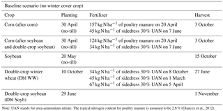
Note: UAN stands for urea-ammonium nitrate. The typical nitrogen content for poultry manure is assumed to be 2.8 % (Glancey et al., 2012).

Table A2 Five general circulation models (GCMs) used to construct the GCM scenario.

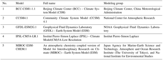
Table A3 Seasonal evapotranspiration (ET, mm ha⁻¹ 10²) under climate sensitivity scenarios (CO₂: carbon dioxide concentration; PCP: precipitation; and TMP: temperature).

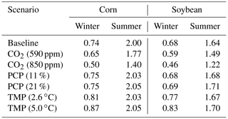
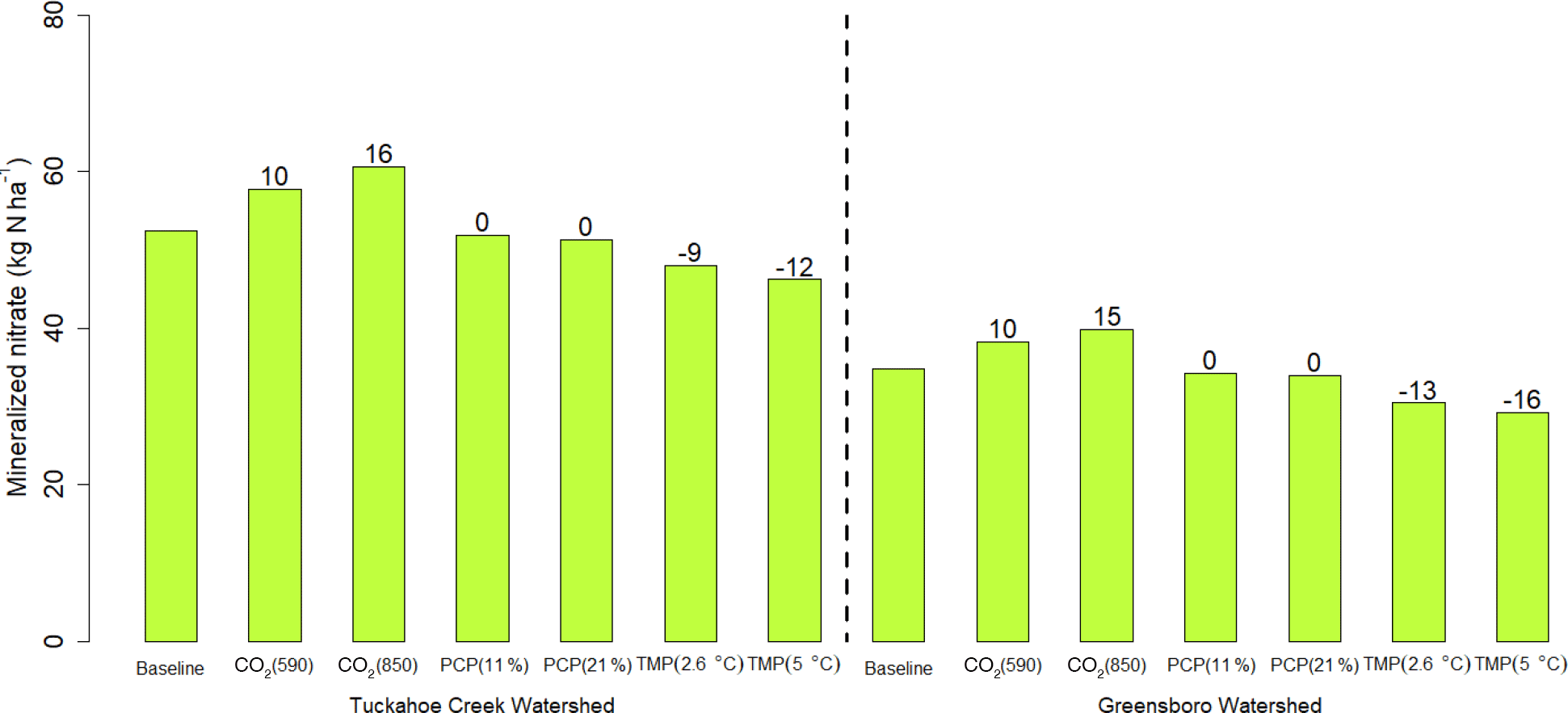
Figure A1 The 14-year average of annual mineralized nitrate during winter seasons (October–March) under the baseline and climate sensitivity scenarios at the watershed scale. Note: the black numerical values above the bar graph indicate the relative changes (%) in hydrologic variables for climate sensitivity scenarios relative to the baseline scenario (relative change (%) = (sensitivity scenarios − baseline) ∕ baseline × 100). PCP and TMP stand for precipitation and temperature, respectively.

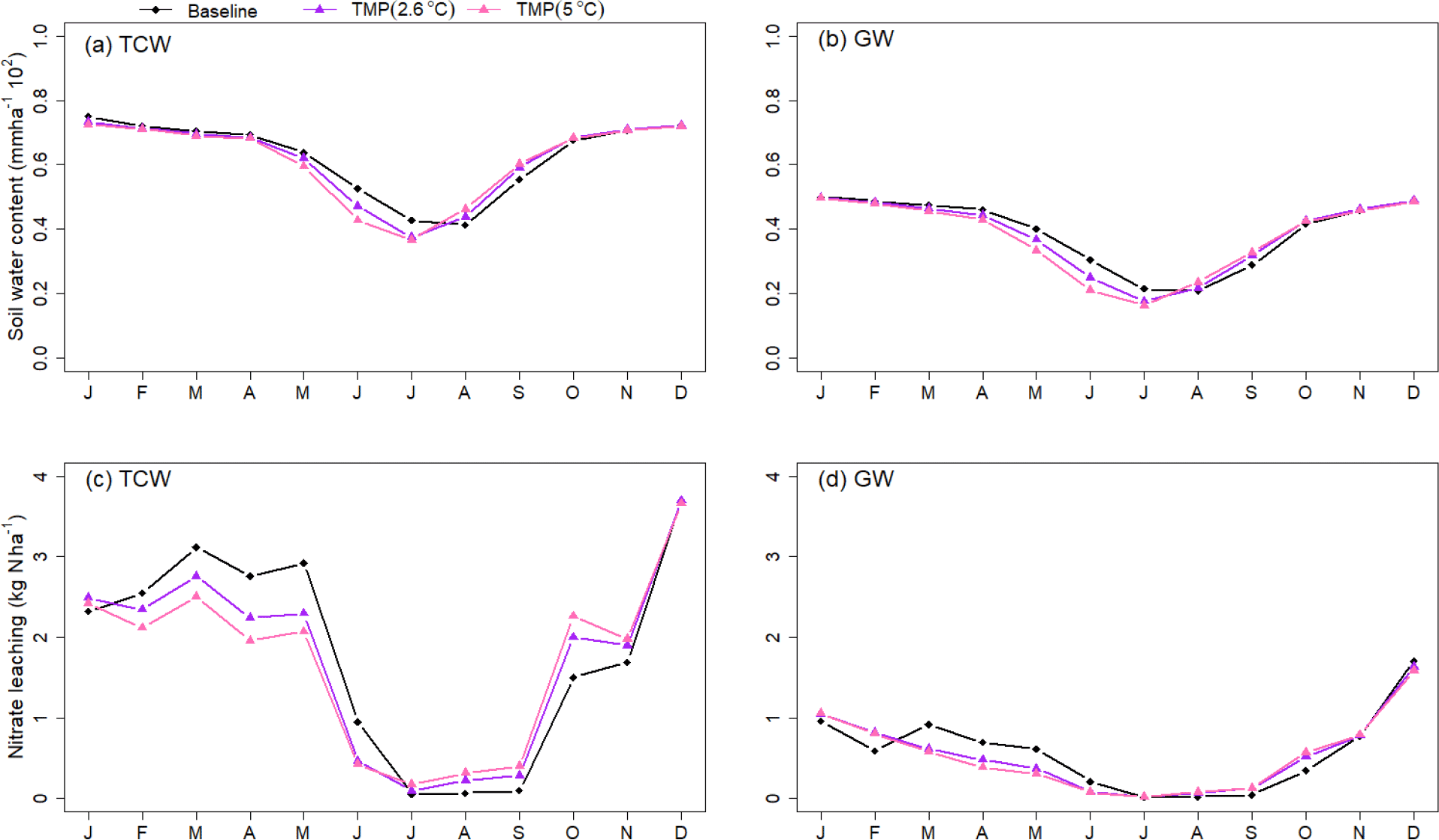
Figure A2 Changes in (a, b) soil water content and (c, d) nitrate leaching under temperature increase for the Tuckahoe Creek Watershed (TCW) and the Greensboro Watershed (GW). Note: TMP stands for temperature.