A conceptual prediction model for seasonal drought processes using atmospheric and oceanic standardized anomalies: application to regional drought processes in China

Reliable drought prediction is fundamental for water resource managers to develop and implement drought mitigation measures. Considering that drought development is closely related to the spatial–temporal evolution of large-scale circulation patterns, we developed a conceptual prediction model of seasonal drought processes based on atmospheric and oceanic standardized anomalies (SAs). Empirical orthogonal function (EOF) analysis is first applied to drought-related SAs at 200 and 500 hPa geopotential height (HGT) and sea surface temperature (SST). Subsequently, SA-based predictors are built based on the spatial pattern of the first EOF modes. This drought prediction model is essentially the synchronous statistical relationship between 90-day-accumulated atmospheric–oceanic SA-based predictors and SPI3 (3-month standardized precipitation index), calibrated using a simple stepwise regression method. Predictor computation is based on forecast atmospheric–oceanic products retrieved from the NCEP Climate Forecast System Version 2 (CFSv2), indicating the lead time of the model depends on that of CFSv2. The model can make seamless drought predictions for operational use after a year-to-year calibration. Model application to four recent severe regional drought processes in China indicates its good performance in predicting seasonal drought development, despite its weakness in predicting drought severity. Overall, the model can be a worthy reference for seasonal water resource management in China.

1 Introduction

Drought is an economically and ecologically disruptive natural hazard that profoundly impacts water resources, agriculture, ecosystems, and basic human welfare (Dai, 2011). In recent years, extreme drought events have had disastrous impacts worldwide. The 2011 eastern African drought led to famine and severe food crises in several countries, affecting over 9 million people (Funk, 2011). As part of the 2011–2014 California Drought, the drought in 2014 alone cost California USD 2.2 billion in damages and 17 000 agricultural jobs (Howitt et al., 2014). China has also suffered from extreme drought events, such as the 2009–2010 severe drought in southwestern China (Yang et al., 2012), 2011 spring drought in the Yangtze River basin (Lu et al., 2014), and 2014 summer drought in northern China (Wang and He, 2015). Because drought is a costly and disruptive natural hazard, reliable drought prediction is fundamental for water resource managers to develop and implement feasible drought mitigation measures. In the present study, drought prediction is restricted to relatively long-term drought, which is associated with season-scale precipitation deficits.

Drought is generally predicted using two types of methods: model-based dynamical forecasting and statistical prediction. Dynamical forecasting primarily relies on computed drought indicators, such as the standardized precipitation index (SPI; McKee and Kleist, 1993), based on forecast precipitation retrieved from seasonal climate forecast systems (Dutra et al., 2013, 2014; Mo and Lyon, 2015; Yoon et al., 2012). Although dynamically predicted precipitation is useful information for drought situations, especially for short-term forecasting 1 month ahead, it also contains high levels of uncertainty and limited skill with respect to long lead times (Wood et al., 2015; Yoon et al., 2012; Yuan et al., 2013). In contrast, statistical drought prediction is an additional source of prospective drought information (Behrangi et al., 2015; Hao et al., 2014). Different from the physical, complex processes in coupled atmosphere–ocean models used for dynamical prediction, statistical drought prediction models are relatively simple but also perform well. They consist of input variables, methodology, and prediction targets (Mishra and Singh, 2011).

Reasons for good and effective performance of statistical models include methodology improvements and drought-related climate indices used as input variables. To date, much attention has been paid to methodology improvements. Taking advantage of probabilistic and temporal-evolution features of input variables, statistical drought prediction models are primarily forced with probability or machine-learning methods, such as the ensemble streamflow prediction (ESP) method (AghaKouchak, 2014), Markov chain- and Bayesian network-based models (Aviles et al., 2015, 2016; Shin et al., 2016), neural network, and support vector models (Belayneh et al., 2014). In addition to method improvement, climate indices represent large-scale atmospheric or oceanic drivers of precipitation, partly responsible for effective model performance. These climate indices include typical atmospheric and oceanic circulation patterns, such as the North Atlantic Oscillation (NAO; Hurrell, 1995) and El Niño–Southern Oscillation (ENSO; Ropelewski and Halpert, 1987), which have been widely used for drought prediction in different seasons and regions (Behrangi et al., 2015; Bonaccorso et al., 2015; Chen et al., 2013; Mehr et al., 2014; Moreira et al., 2016).

Climate indices, such as the NAO index and NINO 3.4 index, are simple, explicit, and widely used. Therefore, they are the primary indices used for drought prediction. Additionally, based on the relationship between drought indices and potential atmospheric or oceanic circulation patterns, some researchers have also discovered large-scale circulation patterns closely related to regional droughts or have structured new drought predictors (Funk et al., 2014; Kingston et al., 2015). For instance, after discovering the two dominant modes of the eastern African boreal spring rainfall variability that are tied to SST fluctuations, Funk et al. (2014) further determined that the first- and second-mode SST correlation structures were related to two SST indices that could be used to predict eastern African spring droughts.

Similarly, potential atmospheric and oceanic circulation patterns, which are closely related to regional droughts, are also used to construct drought predictors in the present study. Considering that the development of drought processes is closely related to the spatial–temporal evolution of large-scale circulation patterns, we constructed predictors based on anomalous spatial patterns. Because precipitation-inducing circulation patterns usually occur in the troposphere, predictors can be built based on sea surface temperature (SST) and 200 and 500 hPa geopotential height (HGT), reflecting information from different levels of the troposphere. Subsequently, all these predictors from different drought processes and the 3-month SPI, updated daily (hereafter, SPI3), were used to calibrate a synchronous stepwise-regression relationship. The model can be forced with dynamically forecast SST and 200 and 500 hPa HGT conditions, indicating that the lead time depends on that of the climate forecast models. Based on predicted prospective 90-day SPI3 curves, we developed angle-based rules for the drought outlook, which can make the drought outlook easily accessible to water resource managers.

Overall, the objective of this study is to build a conceptual prediction model of seasonal drought processes. The essential and important steps are to (1) structure predictors on the basis of drought-related atmospheric and oceanic circulation patterns, (2) build the synchronous statistical predictor-SPI3 relationship forced with reanalysis and operationally forecast datasets, (3) simulate and predict four severe seasonal drought processes in China to investigate model performance, and (4) propose an objective angle-based method for drought outlook.

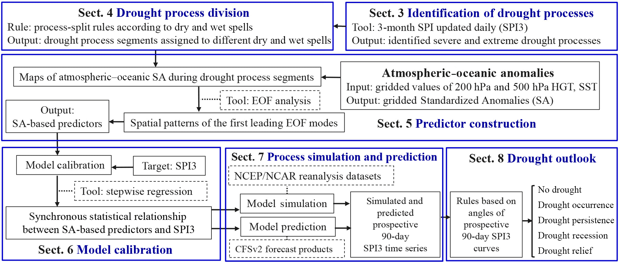
Figure 1 A brief introduction of the sequential procedures described in the sections of this study for drought prediction model construction.

Considering the proposed conceptual model consists of several important parts, a brief but general introduction with sequential procedures is presented (Fig. 1), prior to specific descriptions in Sects. 3–8. In Sect. 3, historical extreme and severe drought processes are identified with SPI3. These drought processes usually go through one or several dry and wet spells, in which precipitation deficit characteristics and circulation patterns vary. Therefore, process-split rules, according to dry and wet spells, are designed to assign drought process segments to different dry and wet spells in Sect. 4. Gridded values in the fields of 200 and 500 hPa HGT and SST are transformed into gridded values of standardized anomalies (SAs) in Sect. 5. Maps of atmospheric–oceanic SAs during drought process segments within the same dry and wet spells are important inputs to the construction of the predictors. After empirical orthogonal function (EOF) analyses are conducted on these SA-based maps, the first leading EOF modes are used to generate predictors (Sect. 5). Further, synchronous statistical relationships between SA-based predictors and SPI3 are calibrated with the stepwise regression method in Sect. 6. The National Centers for Environmental Prediction/National Center for Atmospheric Research (NCEP/NCAR) reanalysis datasets and the NCEP Climate Forecast System Version 2 (CFSv2) operational forecast datasets are used to force the synchronous statistical relationship. Simulated and predicted 90-day prospective SPI3 time series are presented in Sect. 7. With the aid of angle-based rules for seasonal drought outlook, simulated and predicted SPI3 time series are transformed to five types of drought outlooks (Sect. 8), which are easily accessible to water resource managers.

In particular, although drought process predictions in northern, eastern, and southwestern China are all the targets in the present study, only the historical drought processes in northern China are used to introduce the model construction and calibration in Sect. 3–6. Similar procedures were also applied to drought processes in eastern and southwestern China. However, for the sake of conciseness, these procedures, together with intermediate results, are not shown in this study.

2 Data

The precipitation data used were the second-version Dataset of Observed Daily Precipitation Amounts at each 0.5^∘ × 0.5^∘ grid point in China for 1961–2014 (http://data.cma.cn/data/detail/dataCode/SURF_CLI_CHN_PRE_DAY_GRID_0.5.html), which was kindly provided by the Climate Data Centre (CDC) of the National Meteorological Information Centre, China Meteorological Administration (CMA). It was initially used to calculate area-averaged precipitation over northern China, eastern China, and southwestern China (Fig. 2), which are the three Chinese drought regions investigated in this study. They cover areas of approximately 0.69, 0.91, and 1.12 million km², respectively. Atmospheric anomalies were diagnosed with respect to the NCEP/NCAR reanalysis datasets, which has a resolution of 2.5^∘ × 2.5^∘ at 17 pressure levels, extending from January 1948 to the present (Kalnay et al., 1996). The National Oceanic and Atmospheric Administration (NOAA) high-resolution SST dataset, with a spatial resolution of 0.25^∘ × 0.25^∘ and extending from September 1981 to present (Reynolds et al., 2007), was used for SST anomaly analysis.

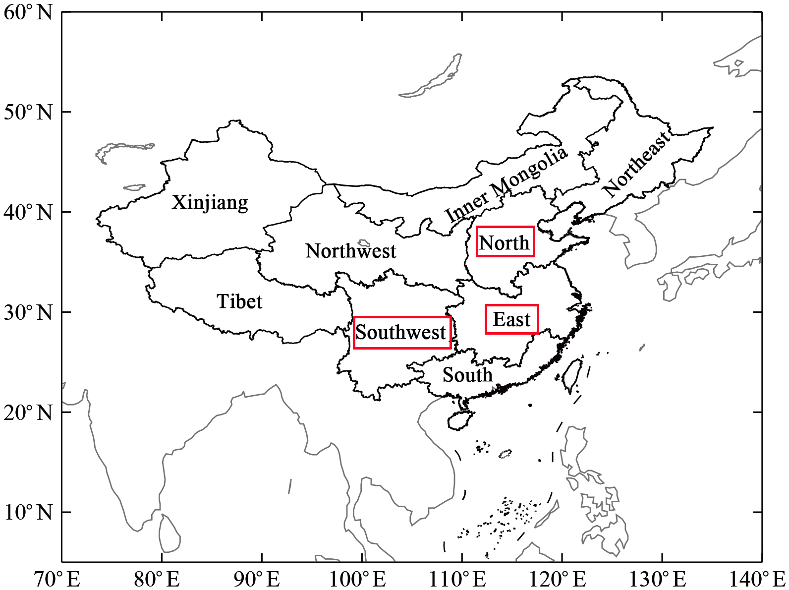
Figure 2 The geographical distribution of China's nine drought regions (black solid curves). The three regions labeled with red boxes are the focus in the present study.

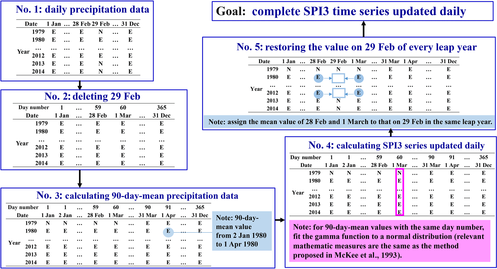
Figure 3 Illustration indicating the steps for calculating daily-updated SPI3. The letter “E” represents value existence, while the letter “N” represents no relevant data.

The NCEP Climate Forecast System Version 2 (CFSv2; Saha et al., 2014) was used to verify operational performance of the proposed conceptual model. Since CFSv2 began on 1 April 2011, some drought processes that occurred before this date were forced with the CFS reforecast output. All the relevant reforecast and forecast datasets are accessible on the website (https://nomads.ncdc.noaa.gov/modeldata/). In particular, we focus on the prospective 90-day seasonal drought process prediction during four severe drought processes in this study. To achieve this, prospective 90-day forecast data subsets for 200 and 500 hPa HGT and SST are retrieved from CFSv2 and CFS products, which are used for the predictor calculation. Details can be found in Sect. S1 in the Supplement.

3 Identification of drought processes

3.1 Three-month SPI updated daily

SPI3 was used as the drought index for seasonal drought recognition and prediction in this study. The calculation period is 1979–2014. The daily area-averaged precipitation datasets were first computed over the three study regions. Traditionally, SPI3 values vary on a monthly timescale, i.e., each month a new value is determined from the precipitation totals of the previous 3 months (McKee and Kleist, 1993). In this study, we chose to update SPI3 daily, which was also recommended by the World Meteorological Organization (2012), i.e., every day a new value is determined from the precipitation totals of the previous 90 days. Specified illustration and details for calculating daily-updated SPI3 are shown in Fig. 3.

3.2 Drought process identification and grade classification

Similar to the rules for SPI grade division recommended by the World Meteorological Organization (2012), the rules in our study are shown in Table 1. Drought processes are identified when the daily SPI3 values are below −0.50 for more than 30 consecutive days.

Each daily SPI3 value for a recognized drought process was assigned to the corresponding SPI3 grade. Starting from the extremely dry grade to the slightly dry grade, the ratio between the duration of a particular SPI3 grade and the total days of the entire drought process is calculated. When the proportion increases beyond 35 %, the corresponding grade is assigned to the entire drought process. For example, as shown in Fig. 4, the proportion of the severely dry days is beyond 35 %. Accordingly, the 2001 summer drought in northern China corresponded to the severe grade.

Table 1 Rules for SPI3 grade classification.

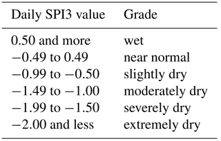
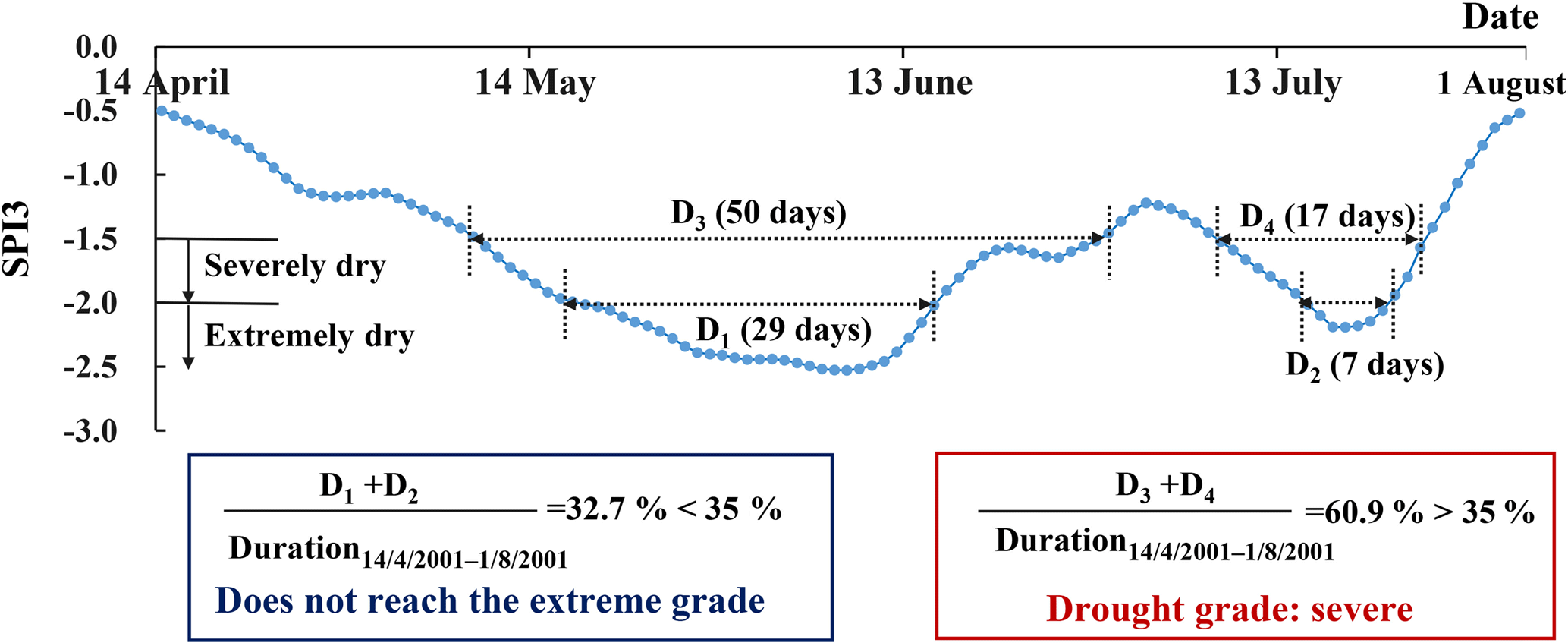
Figure 4 An example of grade classification for one complete drought process: the 2001 summer drought in northern China.

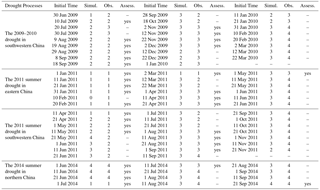
Therefore, we identified severe and extreme drought processes for 1979–2008 in northern China. As shown in Table 2, persistent drought periods from 1997 to 2002 in northern China were found, in agreement with other associated studies (Rong et al., 2008; Wei et al., 2004). Relevant results of identified drought processes in eastern and southwestern China are not shown in the paper.

4 Drought process division according to dry and wet spells

Identified drought processes usually go through one or several dry and wet spells. Different dry and wet spells usually correspond to various precipitation deficit characteristics and atmospheric–oceanic circulation patterns. Therefore, we divided drought processes into different segments according to dry and wet spells, in order to further analyze atmospheric–oceanic anomalies during drought segments within the same dry and wet spells. Additionally, SPI3 on the start date of an identified drought process indicates that SPI3 is initially less than −0.5 and a severe drought process indeed follows, which actually reflects drought-inducing precipitation information for the previous 90 days. Therefore, the start date of the drought process is advanced to the past 90th day, preceding the drought process division. This measure can contribute to introducing early drought-inducing information to predictor construction.

Table 2 Identified severe and extreme drought processes from 1979 to 2008 in northern China.

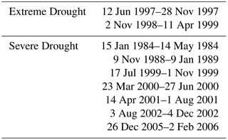
Table 3 Dates of dry and wet spells and their associated proportions of annual total precipitation in northern China. Both Wet–Dry and Dry–Wet represent corresponding transition spells.

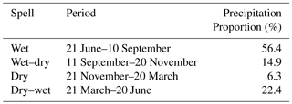
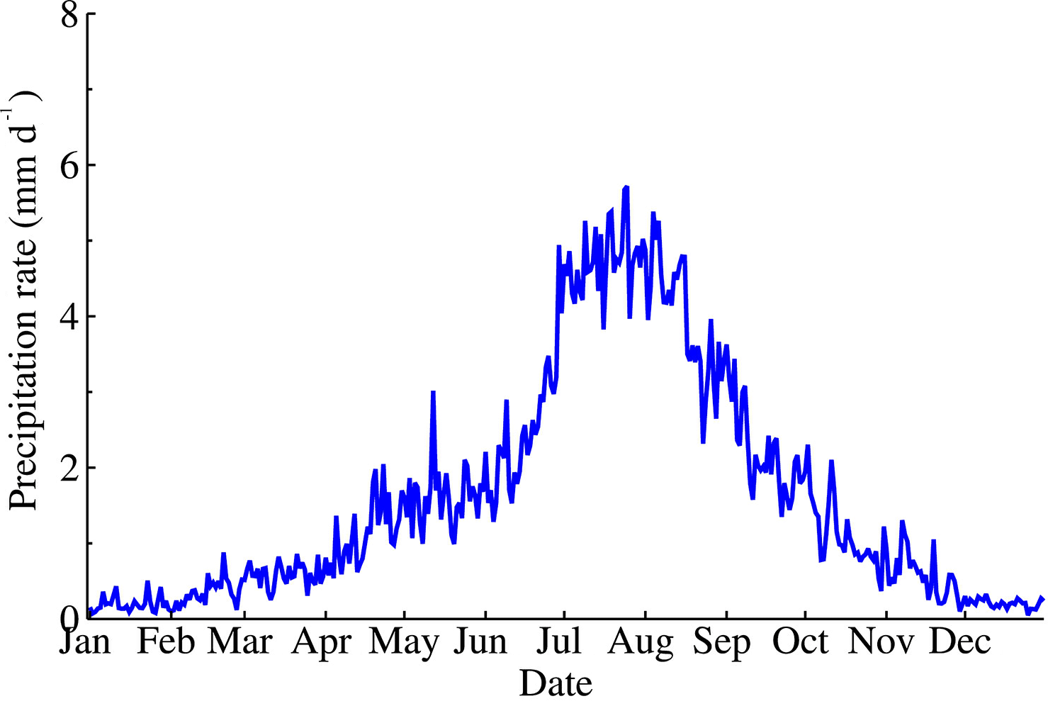
Figure 5 Temporal evolution of daily precipitation rate in northern China, averaged from 1961 to 2010.

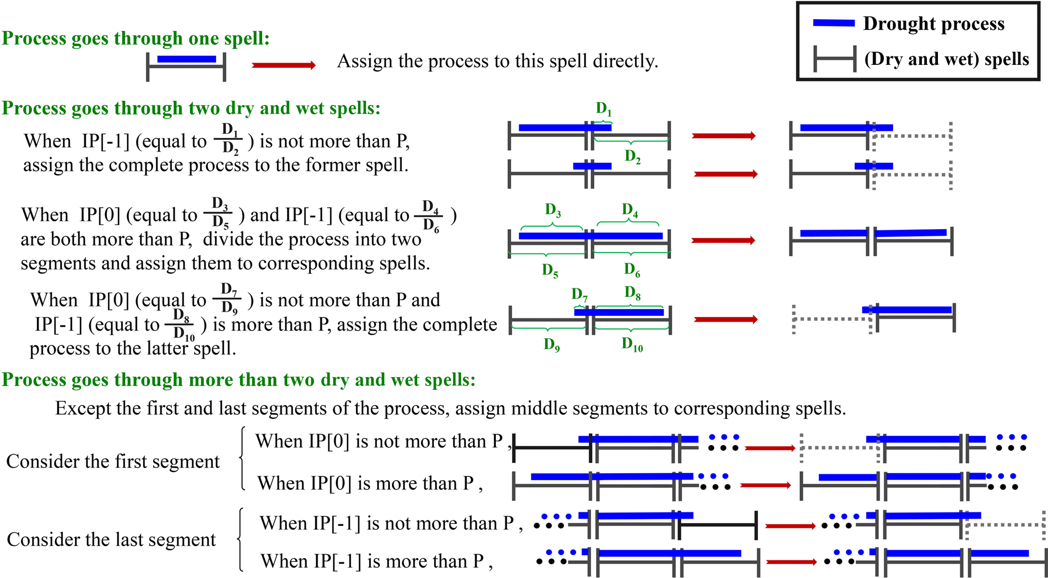
Figure 6 Process-split rules for one drought process according to dry and wet spells. IP represents intersection proportion, while P refers to critical proportion. The terms “IP[0]” and “IP[−1]” express the IP at the start and end segments, respectively.

Table 4 Drought process segments assigned to dry and wet spells during 1979–2008 in northern China.

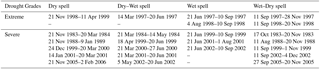
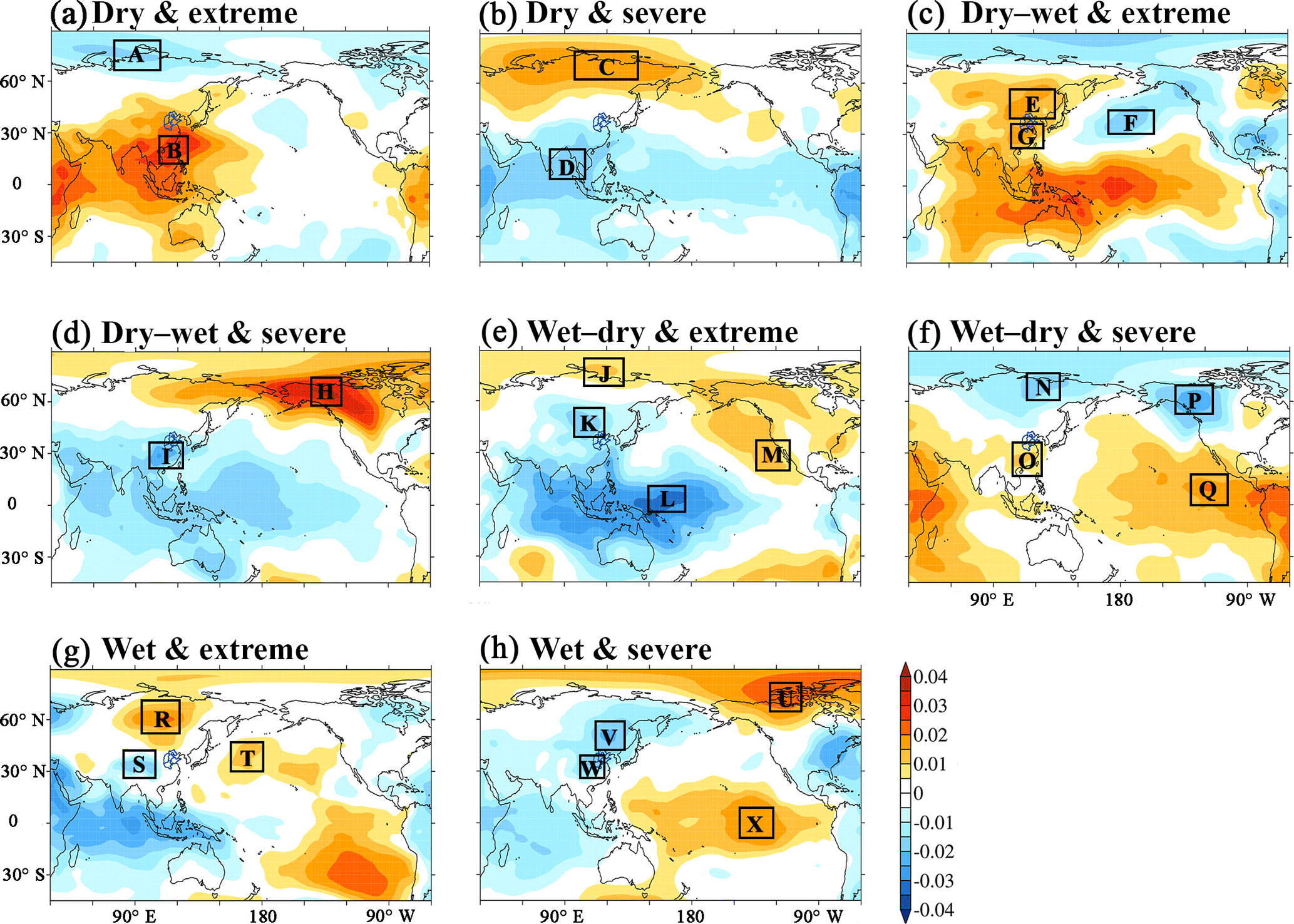
Figure 7 The first leading empirical orthogonal function (EOF) modes of standardized anomalies (SAs) for 500 hPa geopotential height fields (HGT) during all severe and extreme drought process segments during different dry and wet spells in northern China, which is the region described with blue curves. The black boxes outline the selected areas used to structure predictors for northern China, while capital letters refer to the selected area codes.

Using northern China as an example, the specified procedures for the division process are as follows. Similar to general seasonal classification, we divided the annual period into four dry and wet spells (Table 3) according to the temporal evolution of the daily precipitation rate in northern China (Fig. 5). It is evident that the wet spell (one-fourth of the annual duration) accounts for over 50 % of total precipitation, while the dry spell (one-third of the annual duration) accounts for about 6 %.

Based on these dry and wet spells, process-split rules (Fig. 6) are constructed using the intersection proportion (IP) and critical proportion (P, set as 40 %). Herein, IP is the proportion of initial segments accounting for relevant dry and wet spells, and the initial segments (e.g., D₁, D₃, and D₄ in Fig. 6) refer to parts of one drought process split with dry and wet spells. As shown in Fig. 6, one complete process is first transformed into several initial segments according to dry and wet spells. Second, “IP[0]” and “IP[−1]” are calculated, which express IP at the start and end segments, respectively. Third, based on a comparison of IP and P results, these initial segments can be assigned to different dry and wet spells.

Following the process-split rules shown in Fig. 6, we divided these drought processes according to dry and wet spells in northern China (Table 3). Detailed procedures of relevant IP calculations and comparisons can be found in Fig. S1 in the Supplement, while final assignments of initial drought segments are shown in Table 4. In addition, to highlight the importance of extreme droughts, severe and extreme drought segments are considered in turn.

5 Predictor construction

5.1 Atmospheric and oceanic standardized anomalies

To describe atmospheric and oceanic anomalies objectively, we chose the SA method. It was first used to effectively identify high-impact weather events (Grumm and Hart, 2001; Hart and Grumm, 2001). Subsequently, the SA method has also provided significant values for the analysis of extreme precipitation events (Duan et al., 2014; Jiang et al., 2016). In the present study, the SA of a meteorological variable was defined in Hart and Grumm (2001), described as

$$\begin{array}{}\text{(1)}& \mathrm{SA}={\displaystyle \frac{X-\mathit{\mu }}{\mathit{\sigma }}},\end{array}$$

where X represents daily grid-point atmospheric–oceanic circulation pattern variables, which are 200 and 500 hPa HGT and SST in this study. The terms μ and σ are the daily grid-point mean value and daily grid-point standard deviation, respectively. The climatological periods are 1979–2008 for 200 and 500 hPa HGT and 1982–2008 for SST, respectively. For example, with respect to one certain grid point, both the mean 1 January 500 hPa HGT value and associated standard deviation are computed on the 1 January 500 hPa HGT datasets observed during 1979–2008 at each grid point.

5.2 The first EOF leading modes of SA

Empirical orthogonal function analysis (Wilks, 2011) is introduced to decompose spatial–temporal datasets of drought-related atmospheric–oceanic SA into spatially stationary coefficients (leading modes) and time-varying coefficients (principal component). Considering that the first leading EOF modes reflect the largest fraction of drought-related atmospheric–oceanic spatial variability, we focus on them in this study. In addition, in order to highlight the importance of extreme droughts, EOF analysis is conducted on atmospheric–oceanic SAs during severe and extreme drought segments. With the same dry and wet spells and drought grade, SA-based maps during all drought process segments are used for EOF analysis. For example, SA-based maps of 500 hPa HGT during all three severe segments during wet spells in northern China (Table 4) are analyzed with the EOF method, and the first EOF lead mode is shown in Fig. 7h. Identical EOF analysis is conducted on atmospheric–oceanic SA of 200 and 500 hPa HGT and SST during all four dry and wet spells in northern China. Relevant results for northern China are shown in Figs. 7, 8, and S2. In addition, the relevant results of EOF analysis for eastern and southwestern China are different, but for the sake of conciseness, they are not shown in the paper.

Table 5 Predictor-structured results based on the first leading empirical orthogonal function (EOF) modes for SAs of 200 hPa HGT, 500 hPa HGT, and SST fields during different dry and wet spells in northern China. Capital letters refer to the code for selected areas in Figs. 7, 8, and S2. In the term “P_XXX,Y”, P, XXX, and Y refer to predictors, atmospheric or oceanic elements, and the code of new predictors, respectively.

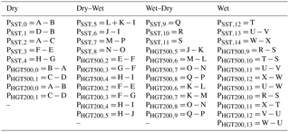
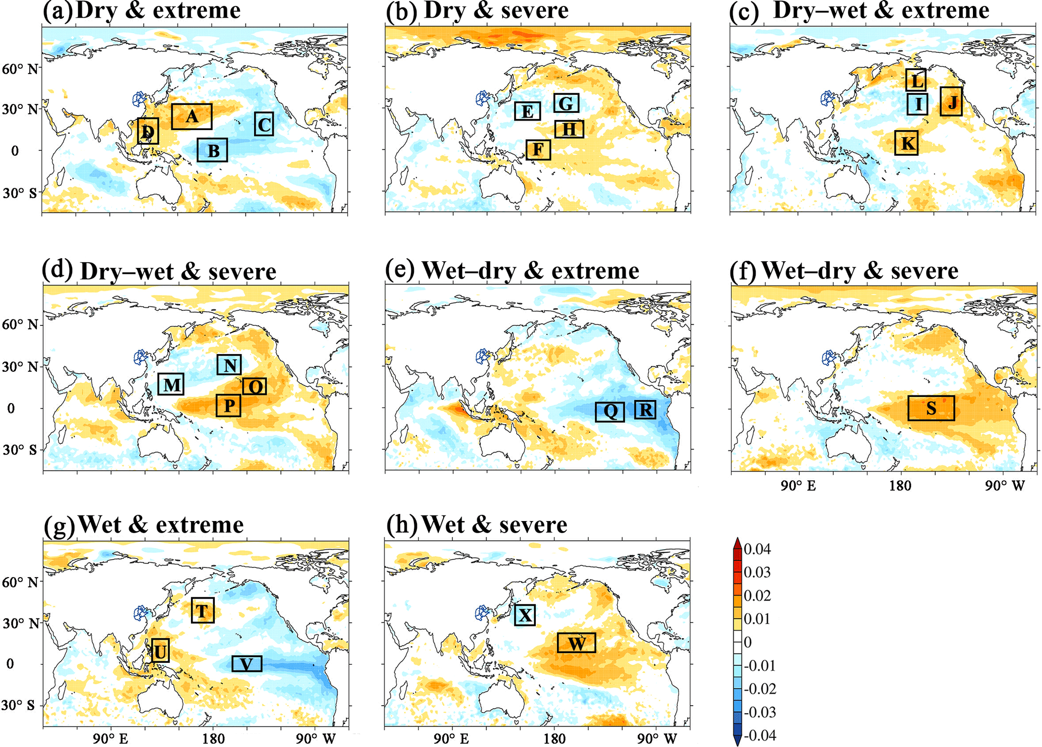
Figure 8 Same as Fig. 7, but for standardized anomalies (SAs) of SST fields associated with droughts in northern China.

5.3 Pattern-based predictor construction

Positive and negative pattern areas in the first EOF leading modes are used to build predictors, which resemble the pattern-based definition of atmospheric teleconnection indices (Wallace and Gutzler, 1981). As shown in Fig. 7a, a large area of positive pattern (region B) occurs over southeastern China, while a negative pattern area (region A) appears to the north of Eurasia. Generally, the predictor is area-averaged over all gridded SA-based variables in selected areas, such as A and B, considering the reversed signs indicated with different colors. Results from the pattern-based predictor construction are shown in Table 5.

Table 6 Statistical parameters of stepwise-regression equations used for prediction during different calibration periods in northern China.

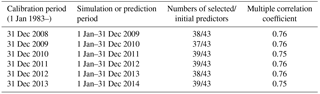
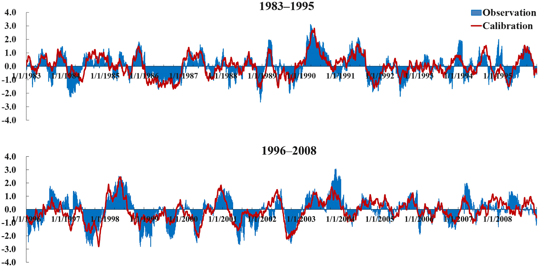
Figure 9 Temporal evolution of observed and calibrated SPI3 during the calibration period between 1 January 1983 and 31 December 2008 in northern China.

As shown in Fig. 7, the spatial pattern of different phases in the 500 hPa HGT fields were adequately considered, including low–high latitude differences (e.g., P_HGT500,0 in Table 5) and ocean–continent differences (e.g., P_HGT500,3 in Table 5). In addition, the spatial pattern of different phases surrounding the prediction-targeted region (e.g., regions R, S, and T in Fig. 7g) was intentionally used to construct predictors, such as P_HGT500,9 and P_HGT500,10 in Table 5. Because the first EOF modes of 200 hPa HGT (Fig. S2) were similar to those of 500 hPa HGT, the specified illustrations were not shown here but were considered in the analysis. Additionally, the positive and negative pattern areas in the Pacific SST SA fields were also used, especially in the subtropical gyre zone (Fig. 8a–d) and El Niño region (Fig. 8e and f). Furthermore, some regions, such as the El Niño Regions R, Q, and S, were separately used for the construction of the predictors. In addition to the predictors constructed for northern China (Table 5), different predictor-structured results for eastern and southwestern China were also obtained but not shown in the paper.

6 Model calibration

6.1 Synchronous statistical relationship

Stepwise regression (Afifi and Azen, 1972) is a method for fitting multiple linear regression models, in which a predictive variable is considered for addition to or subtraction from a set of explanatory variables according to statistically significant extent or loss. In this study, it is used to build the synchronous statistical relationship between all 90-day-accumulated SA-based predictors and the prediction target SPI3. SA-based predictors are calculated with the NCEP/NCAR reanalysis dataset (Kalnay et al., 1996). Essentially, the conceptual model, aimed at seasonal drought process prediction, is a synchronous stepwise relationship.

6.2 Rolling calibration year by year

To meet the practical requirements of operational service departments, model calibration is also running year by year (Table 6). For example, the seasonal drought prediction model, calibrated from 1 January 1983 to 31 December 2011, is used for initial daily prediction time in the entire 2012 year. For every initial drought prediction in the year 2013, the corresponding drought model is calibrated from 1 January 1983 to 31 December 2012. In addition, detailed information about selected predictors and relevant coefficients can be found in Table S1 in the Supplement.

The calibration period increases year by year, therefore, the number of samples used for calibration also increases year by year. Multiple correlation coefficients in six drought prediction models are no less than 0.75. Statistical parameters and their total numbers show slight changes across the six calibration experiments (Table 6). Furthermore, calibrated SPI3 curves are almost consistent with the observation data (Fig. 9), especially with respect to turning points and trends. Different parameter sets and results of model calibration for eastern and southwestern China are not shown in the paper.

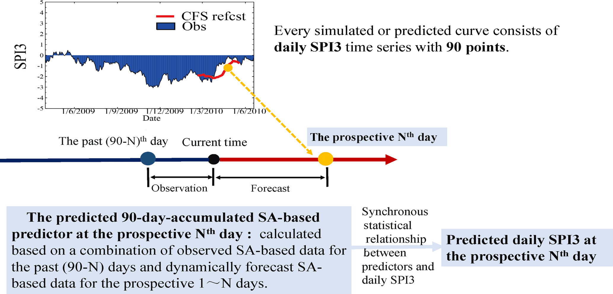
Figure 10 Illustration about how to calculate the prospective 90-day daily SPI3 time series. ”Reforecast” is denoted by ”refcst”.

7 Drought process simulation and prediction

7.1 Model forcing

Because the conceptual model is essentially a synchronous statistical relationship, the model itself has no lead time. Therefore, model simulation and prediction have to be further forced with reanalysis and forecast datasets. During the periods of model simulation, the synchronous statistical relationship is forced with the NCEP/NCAR reanalysis dataset. For model prediction, it is operationally forced with CFSv2 forecast datasets, together with the NCEP/NCAR reanalysis dataset. Therefore, the lead time for the conceptual model depends on that of the climate forecast models.

In particular, because we focus on the prospective 90-day drought process prediction (predicted daily SPI3 time series with 90 points), it is necessary to illustrate how to calculate every forecast point (daily SPI3). As shown in Fig. 10, predicted daily SPI3 at the prospective Nth day is originally based on a combination of observed and dynamically forecast SA-based data. The computation of these SA-based data follow Sect. 5.1, and the observed data are also retrieved from the NCEP/NCAR reanalysis data. In addition, when the lead time is longer, more dynamically forecast data are included and corresponding daily SPI3 value contains larger uncertainty.

Figure 11 Temporal evolution of observed and simulated SPI3 processes during the period from 1 January 2009 to 31 December 2014. The black boxes in (a)–(c) indicate the 2014 summer and autumn drought in northern China, 2011 spring drought in eastern China, 2009–2010 drought in southwestern China, and 2011 summer drought in southwestern China. Red curves refer to simulated SPI3, while curves filled with light blue represent observed SPI3.

7.2 Drought processes simulated with the NCEP/NCAR reanalysis datasets

To assess model performance of severe seasonal droughts, we take four recent drought processes in southwestern China, eastern China, and northern China as examples. First, southwestern China experienced two severe droughts (the black boxes in Fig. 11c). Although the simulated SPI3 does not reach its peak during the 2009–2010 drought, it indicates the state transformation from drought occurrence to persistence and eventually to relief. In terms of the 2011 summer drought in the southwestern China, the simulated SPI3 indicates that the state remains wet and gradually becomes wetter, indicating no valuable information consistent with observations. Nevertheless, during the phase of drought recession, the simulated development is quite similar to the observed development. This comparison indicates that the conceptual model performs well in development but is weak in severity. This distinct feature also appears in the simulation of the 2011 drought in eastern China (the black box in Fig. 11b) and 2014 drought in northern China (the black box in Fig. 11a).

Figure 12 Simulation and prediction results of four recent severe drought processes in China. Every unfilled curve represents simulated or predicted prospective 90-day SPI3, with an interval of initial prediction time of about 10 days. The curves filled with blue refer to observed SPI3. Dark red and bright red curves refer to SPI3 predicted with CFSv2 and CFS products, respectively. Light green curves represent SPI3 simulated with the NCEP/NCAR reanalysis datasets. Every simulated or predicted curve consists of daily SPI3 time series with 90 points. ”Reforecast” is denoted by ”refcst”.

7.3 Drought processes predicted with the CFSv2 forecast datasets

Compared with drought simulation, operationally predicted results may bring some uncertainties into the prospective drought processes. As shown in Fig. 12b, predicted curves perform worse than the simulated curves near the peak of the 2011 eastern China drought, as the prospective observation tendency is rising rather than decreasing. However, in the other three droughts, the predicted curves are good at indicating drought development to some different degrees, resembling the simulated results quite well. For example, the presented operationally reforecast curves indicate drought occurrence, persistence, and relief during the 2009–2010 drought in southwestern China (Fig. 12a).

8 Drought outlook

8.1 Angle-based rules

Compared with the predicted prospective SPI3 time series, the drought outlook is a convenient and valuable attachment product for water resource managers. To create the drought outlook, angle-based rules are developed to transform the predicted prospective 90-day SPI3 curves into different drought tendencies. Three essential technical points are as follows.

First, some variables must be defined to describe drought development. Similar to the slope of curves, angles of predicted 90-day SPI3 curves are used to describe the prospective drought situation. Generally, positive angles of SPI3 curves indicate wetter tendencies, while negative angles represent drier tendencies.

The second is two general classifications of drought outlook on the basis of the current drought situation. For no current drought (see sketch map I in Fig. 13), the prospective situation tends to be no drought or drought occurrence. In this case, a critical angle α₁ can be used to help distinguish between these two types of drought outlook. A calculated SPI3 curve angle α that is less than α₁ results in the prospective development of drought occurrence; otherwise, the non-drought situation persists. Similarly, for a current condition of being in drought (see sketch map II in Fig. 13), a comparison of critical angles α₂ (equal to zero) and α₃ defines the other three types of drought outlook, which are drought persistence (α less than α₂), drought recession (α more than α₂, but less than α₃), and drought relief (α more than α₃).

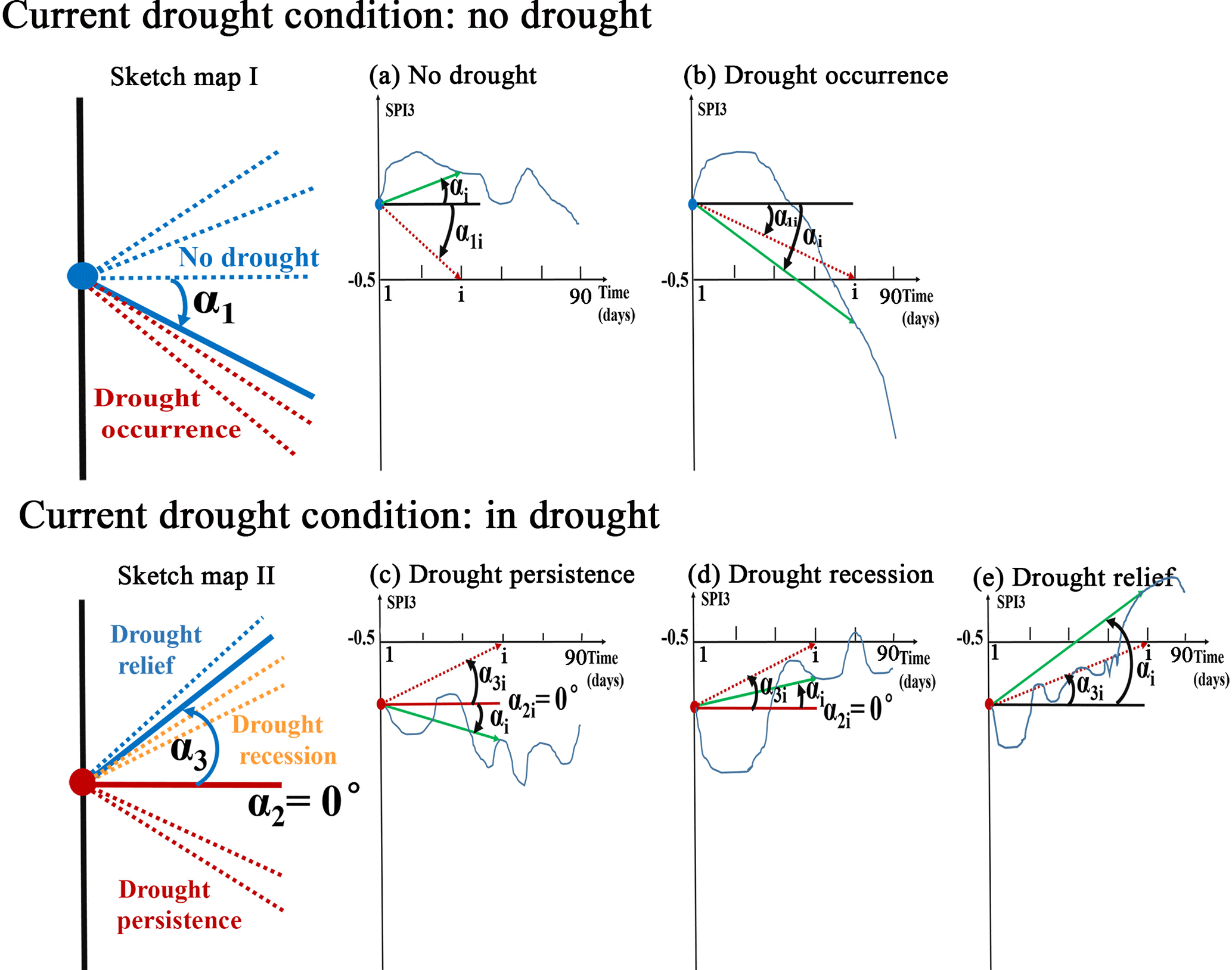
Figure 13 Rules of drought outlook based on angle comparison of prospective 90-day SPI3 curves. Sketch maps I and II show general drought outlook based on the current drought situation. Panels (a)–(b) and (c)–(e) express different situations of drought outlook associated with the rules regarding critical angles in Table 7.

Table 7 Specific rules for drought outlook based on angle comparison. R1 represents the ratio of days when α_i is less than the critical angle α_1i(α_3i) to the total 90 days. R2 represents the proportion of specific days in the period to the predicted prospective 46–90 days. In R2 calculation, these specific days meet the criteria that α_i is greater than critical angle α_3i.

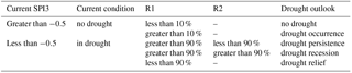
Table 8 Simulation assessment of recent severe drought processes in China forced with the NCEP/NCAR reanalysis datasets. The numbers 0–4 in the below table represent different drought states: no drought (0), drought occurrence (1), drought persistence (2), drought recession (3), and drought relief (4). As well as this, the abbreviation “Simul.” and “Obs.” represent the simulated and observed drought outlooks, respectively. The abbreviation “Assess.” in the column refers to whether the simulation and observation agree or not.

Third, it is necessary to explain the practical calculation for curve angles and how to conduct an angle-based drought outlook. Except the constant critical angle α₂ (equal to zero), both α₁ and α₃ represent angles between the horizontal line and arrow from the original point (initial prediction time) to the points on the time axis (see red dashed arrowed lines in Fig. 13a–e). Similarly, α represents angles between the horizontal line and arrow from the original point to the points on the predicted SPI3 curve (see green solid arrowed lines in Fig. 13a–e). However, considering the predicted period of SPI3 time series is prospectively 90 days, curve angle α_i and critical angles α_1i, α_2i and α_3i ($i=\mathrm{1},\mathrm{2},\mathrm{\dots },\mathrm{90}$) can be calculated. Finally, according to the angle-based rules shown in Table 7, a drought outlook can be performed.

8.2 Simulated and predicted results

Following the method in Sect. 8.1, drought outlook is conducted based on angle comparison of the simulated prospective 90-day SPI3 curve (Table 8). Simulations at every initial time are real-time corrected with the current situation. In terms of the 2009–2010 drought in southwestern China and the 2011 summer drought in eastern China, the simulated drought outlook performs well with respect to drought occurrence, persistence, and recession before 2 December 2009 and 1 May 2011. In addition, the simulation of the 2011 drought in southwestern China performs well in August 2011. The 2014 summer drought in northern China lasts for a relatively short time, resulting in an observed drought outlook that maintains a state of drought relief during the first month of the drought process. Even so, the simulation can also capture it. Additionally, these four drought outlooks remain weak in simulating the development of drought relief after 31 January 2010, 11 May 2011, 11 September 2011, and 21 July 2014, respectively. Weak performance in simulating severity leads to the development of drought recession rather than drought relief.

For predicted drought outlooks, operationally predicted results (Table 9) in southwestern China and eastern China are relatively similar to the simulated ones (Table 8). In comparison, predicted drought outlook during the first month of the 2014 drought in northern China performs worse than simulated results.

9 Discussion

Considering that the development of drought processes is closely related to the spatial–temporal evolution of atmospheric and oceanic anomalies, a conceptual prediction model of seasonal drought processes is proposed in our study. Despite its weakness in predicting drought severity, the model performs well in simulating and predicting drought development. Because the proposed model is a new attempt, several associated discussion issues are as follows.

Table 9 Same as Table 8 but for predicted results forced with the operational output from CFSv2. The abbreviation “Predi.” represents the predicted drought outlook. The abbreviation “Assess.” in the column refers to whether the prediction and observation agree or not.

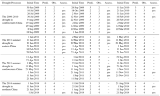
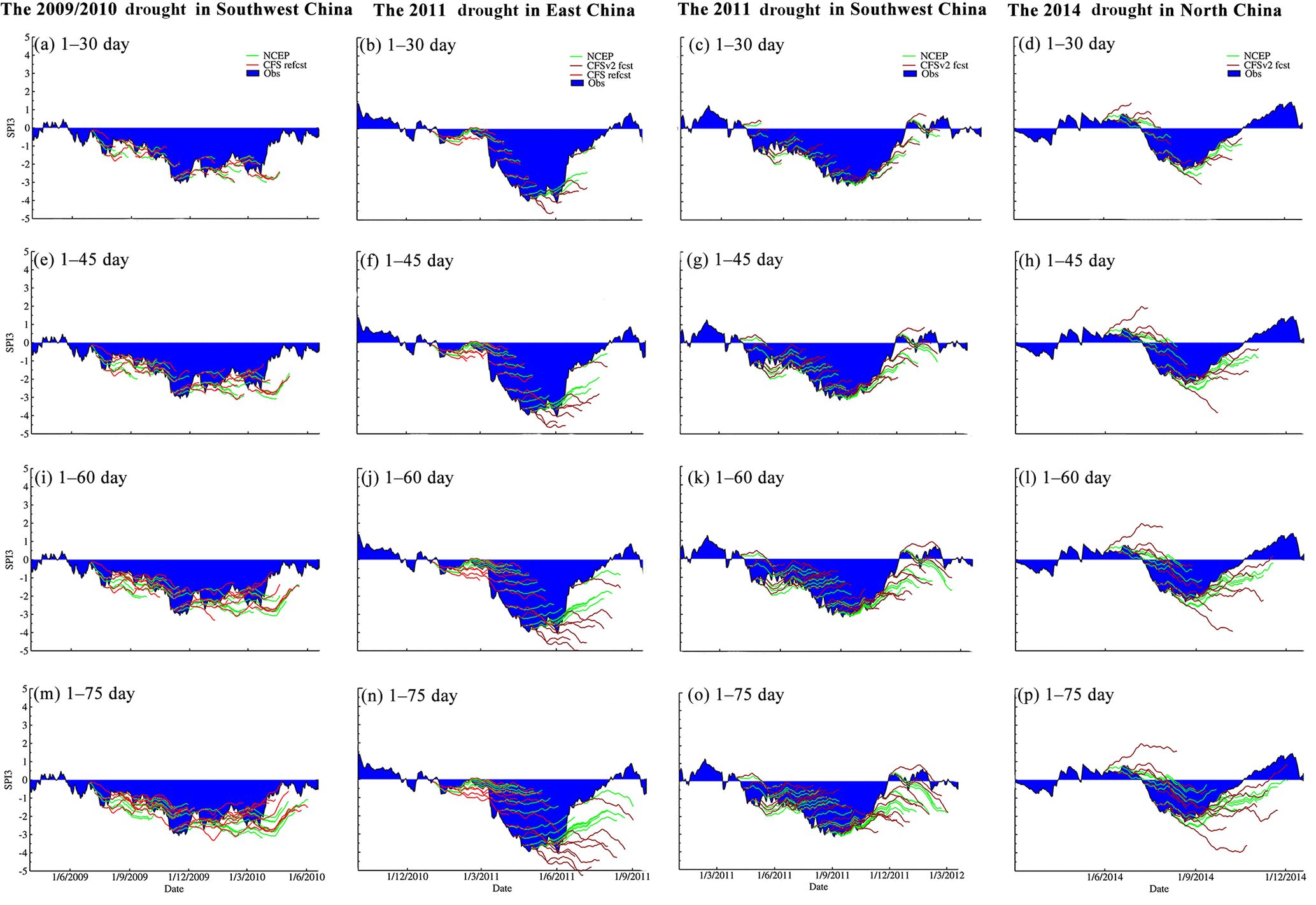
Figure 14 Same as Fig. 12 but for different predicted periods, which are namely the prospective (a)–(d) 1–30-day, (e)–(h) 1–45-day, (i)–(l) 1–60-day, and (m)–(p) 1–75-day periods. “Reforecast” is denoted by “refcst” and “forecast” by “fcst”.

First, process prediction and outlook of seasonal drought are the focus of our study. To date, a considerable number of studies have focused on predicting discrete drought classes (Aviles et al., 2016; Bonaccorso et al., 2015; Chen et al., 2013; Moreira et al., 2016) and the probability of drought occurrence within certain classes (AghaKouchak, 2014, 2015; Hao et al., 2014). Compared with these studies, prediction of regional drought processes is another valuable attempt, which is beneficial from the moving window of SPI3 extended from 1 month to 1 day. It performs relatively well in predicting the development of seasonal drought processes (Fig. 12). In addition, it can indicate drought occurrence, persistence, and relief relatively well (Tables 8 and 9), which is meaningful for seasonal water resource management.

Second, the proposed model is essentially one stepwise-regression equation. Despite its simplicity, it incorporates drought-related spatial and temporal information as integrally as possible. Because precipitation-related synoptic systems appear in the troposphere, SST, 500 hPa HGT, and 200 hPa HGT are chosen as representatives of the low, middle, and upper levels of the troposphere, respectively. Furthermore, all drought process segments assigned to different dry and wet spells are used for EOF analysis within the same dry and wet spells (shown in Sect. 5.2). Therefore, adequate drought-related spatial–temporal information has been included in these drought predictors.

Third, the reasons for acceptable performance of operationally predicted results need to be illustrated. Compared with those forced with the NCEP/NCAR reanalysis datasets (green curves in Fig. 12), the predicted developments of drought processes forced with CFSv2 or CFS datasets (red curves in Fig. 12) are relatively similar, especially with respect to the former segment of every predicted prospective 90-day SPI3 curve. Essentially, the 90-day-accumulated SA-based predictors strengthen the good performance of operational use. This indicates that observed information from atmospheric and oceanic anomalies are involved to different degrees (Fig. 10). With the incorporation of observed data, its operational application provides relatively accurate and valuable information. However, it is also worthwhile to investigate how changing the length of the predicted period can make predicted drought processes relatively accurate and acceptable, such as the prospective 1–30-day or the prospective 1–60-day periods. The relevant comparison results with different predicted periods are shown in Fig. 14. It appears that the 2009–2010 drought in southwestern China and 2014 drought in northern China can be predicted and simulated well even for the prospective 1–75-day period. In contrast, the prospective 1–45-day period may be a feasible and acceptable lead time for simulation and prediction of the 2011 droughts in southwestern China and eastern China, after which the simulated and predicted developments clearly change.

Fourth, the weak performance in predicting the severity of drought, including drought peak and drought relief, is an important issue. Similar to the concluding remarks regarding a probabilistic drought prediction model, the weak performance in predicting the severity of the drought peak is due to the typical problem of an inherent averaging effect depressing the extremes (Behrangi et al., 2015). With the help of real-time correction from operational application, the prediction of drought peaks can be improved. In addition, the prediction of drought relief should also be considered. As listed in both Tables 8 and 9, the simulated and predicted results for drought relief are unsatisfying. This weak performance may be associated with precipitation-causing weather patterns during drought relief. They are unsteady and change dramatically compared with those features during drought persistence. Because the period of drought relief is a relatively short phase of the drought process, the relevant information may not be involved in the first EOF modes (Sect. 5.2). Generally, three measures for potential improvement are as follows. (1) More secondary EOF modes, including precipitation-causing circulation patterns during drought relief, can be incorporated when building initial predictors. (2) The rapid change index (Otkin et al., 2015) could be introduced to describe temporal changes during drought relief on subseasonal timescales. (3) The empirical factor can be introduced to improve drought-relief prediction. The predicted SPI3 during the phase of drought relief could be multiplied by empirical factors to strengthen drought relief development.

Fifth, it is necessary to explain the method of predictor construction. The predictor-structured method in our study is similar to the definition of teleconnection indices (Wallace and Gutzler, 1981). It is more goal-directed, because these structured predictors are directly related to synchronous atmospheric–oceanic anomalous circulation patterns during different drought segments within the same dry and wet spells. However, to design geographical ranges of anomalous areas and combine them is subjective, which leads to considerable uncertainties. Accordingly, an objective anomaly-recognized method with explicit critical values needs to be developed. This will contribute to auto-run feasibility of this conceptual prediction model without artificial interaction.

The sixth issue to illustrate is synchronous SST anomalies used in EOF analysis and model construction. Traditionally, SST anomalies a few months ahead influence the subsequent regional droughts. However, it is also feasible and common that synchronous SST anomalies are used in the investigation of regional drought events in southwestern China (Feng et al., 2014), the Yangtze River basin (Lu et al., 2014), and northern China (Wang and He, 2015), which may shape synchronous drought-related circulation patterns. In addition, this is convenient for operational application, while forecast SST and 200 and 500 hPa HGT can be retrieved together from CFSv2 products simultaneously.

Finally, the timescale of the drought index needs to be explained. SPI3 is the index used for drought identification and prediction in the study, which provides a seasonal estimation of precipitation and tends to be a good indication of soil moisture conditions as the growing season begins in some primary agricultural regions worldwide (WMO, 2012). However, to meet operational requirements of seasonal hydrological forecasting, the indices such as 6-month up to 24-month SPI can be also used for hydrological drought analyses and applications (WMO, 2012). With the increasing timescale of SPI, its lead time with given accuracy requirements might be longer, together with the smoother temporal evolution. Accordingly, atmospheric and oceanic anomalies used for model calibration need to be changed from 90-day accumulated to 6- or 24-month accumulated.

10 Conclusions

Drought prediction is fundamental for seasonal water management. In this study, we constructed a conceptual prediction model of seasonal drought processes based on synchronous standardized anomalies of 200 and 500 hPa geopotential height and sea surface temperature; we considered that drought development is closely related to the spatial–temporal evolution of large-scale atmospheric–oceanic circulation patterns. We used northern China as an example to introduce the method and used four recent severe regional drought processes in China for model application. This model can be used for seamless drought prediction and drought outlook, forced with seasonal climate forecast models. The main process is as follows. (1) A 3-month SPI updated daily (SPI3) was used to capture severe and extreme drought processes. (2) Empirical orthogonal function analysis was applied to SA of 200 and 500 hPa HGT and SST during drought process segments within the same dry and wet spells. Subsequently, spatial patterns of the first EOF modes were used to structure SA-based predictors. (3) The synchronous stepwise-regression relationship between SPI3 and all 90-day-accumulated SA-based predictors were calibrated using the NCEP/NCAR reanalysis datasets. (4) To achieve a prospective 90-day drought outlook, we further developed an objective method based on angles of the predicted prospective 90-day SPI3 curves. (5) Finally, simulation and prediction of seasonal drought processes, together with drought outlook, were forced with the NCEP/NCAR reanalysis datasets and the NCEP Climate Forecast System Version 2 (CFSv2) operationally forecast datasets, respectively. Model application during four recent severe drought processes in China revealed that the model is good at development prediction but weak in severity prediction. These results indicate that the proposed conceptual drought prediction model is another potentially valuable addition to current research on drought prediction.