Global 5 km resolution estimates of secondary evaporation including irrigation through satellite data assimilation

A portion of globally generated surface and groundwater resources evaporates from wetlands, waterbodies and irrigated areas. This secondary evaporation of “blue” water directly affects the remaining water resources available for ecosystems and human use. At the global scale, a lack of detailed water balance studies and direct observations limits our understanding of the magnitude and spatial and temporal distribution of secondary evaporation. Here, we propose a methodology to assimilate satellite-derived information into the landscape hydrological model W3 at an unprecedented 0.05^∘, or ca. 5 km resolution globally. The assimilated data are all derived from MODIS observations, including surface water extent, surface albedo, vegetation cover, leaf area index, canopy conductance and land surface temperature (LST). The information from these products is imparted on the model in a simple but efficient manner, through a combination of direct insertion of the surface water extent, an evaporation flux adjustment based on LST and parameter nudging for the other observations. The resulting water balance estimates were evaluated against river basin discharge records and the water balance of closed basins and demonstrably improved water balance estimates compared to ignoring secondary evaporation (e.g., bias improved from +38 to +2 mm yr⁻¹). The evaporation estimates derived from assimilation were combined with global mapping of irrigation crops to derive a minimum estimate of irrigation water requirements (I₀), representative of optimal irrigation efficiency. Our I₀ estimates were lower than published country-level estimates of irrigation water use produced by alternative estimation methods, for reasons that are discussed. We estimate that 16 % of globally generated water resources evaporate before reaching the oceans, enhancing total terrestrial evaporation by 6.1×10¹² m³ yr⁻¹ or 8.8 %. Of this volume, 5 % is evaporated from irrigation areas, 58 % from terrestrial waterbodies and 37 % from other surfaces. Model-data assimilation at even higher spatial resolutions can achieve a further reduction in uncertainty but will require more accurate and detailed mapping of surface water dynamics and areas equipped for irrigation.

1 Introduction

The generation of surface and groundwater resources is commonly conceptualized one-dimensionally as the net difference between precipitation, evaporation (including transpiration) and soil storage change. However, some part of the generated “blue” water (Falkenmark and Rockström, 2004) subsequently inundates floodplains, accumulates in wetlands and freshwater bodies or is extracted for irrigation. A fraction of that water will evaporate in this second instance. This “secondary evaporation” directly reduces the remaining blue water resources available for ecosystems and economic uses downstream but also increases the use of water by terrestrial ecosystems before discharging into the oceans. At the global scale, our understanding of the magnitude and spatiotemporal distribution of secondary evaporation is limited by a lack of detailed water balance studies and direct observations. Until recently, land surface models have ignored lateral water transport and secondary evaporation altogether or provide a rudimentary description. This is understandable, given the complexity and computational challenge in simulating the lateral redistribution and secondary evaporation of water at the global scale. However, it is increasingly clear that the lateral redistribution of water cannot be ignored in global water resources analyses (Oki and Kanae, 2006; Alcamo et al., 2003), carbon cycle analyses (Melton et al., 2013) and regional and global climate studies (e.g., Thiery et al., 2017).

Even approximate numbers on the importance of secondary evaporation in the global water cycle are not available. Oki and Kanae (2006) derived global bulk estimates of gross evaporation from lakes, wetlands and irrigation (combined 10.1×10¹² m³ yr⁻¹) but their estimate was based on modelling only and included both primary and secondary evaporation. There have been some studies estimating irrigation water requirements at the global scale (Döll and Siebert, 2002; Wada et al., 2014; Siebert and Döll, 2010), but these studies were based on idealized modelling, did not attempt to separate between primary and secondary evaporation and did not consider other sources of secondary evaporation.

There have been attempts to use satellite observations to estimate the importance of secondary evaporation at a regional scale. For example, Doody et al. (2017) used MODIS-based evaporation estimates (Guerschman et al., 2009) over Australia to delineate areas receiving lateral inflows. They used ancillary data to attribute these to surface water inundation, irrigation and groundwater-dependent ecosystems. At the global scale, Wang-Erlandsson et al. (2016) used satellite-based evaporation estimates from several sources to infer rooting depth, which provided some insight into the spatial distribution of surface and groundwater-dependent ecosystems.

Historically, three contrasting approaches have been followed to estimate evaporation. These are water balance modelling, inferencing from land surface temperature (LST) remote sensing and estimating based on the remote sensing of vegetation. All three approaches rely on meteorological data and effectively involve a land surface model of some description, albeit of variable complexity. Hybrids between the three approaches have also been developed over time to mitigate respective weaknesses (Glenn et al., 2011). For example, the dynamic simulation of the soil water balance can provide a valuable constraint on satellite-based evaporation estimates in water-limited environments, provided that precipitation is the only source of water for evaporation and accurate precipitation estimates are available (Glenn et al., 2011; Miralles et al., 2016). However, where there are additional sources of water or unexpected soil moisture dynamics, applying this constraint can degrade evaporation estimates.

Beyond dynamic hydrological models, evaporation products based more closely on the remote sensing of vegetation implicitly account for the effect of lateral water redistribution on transpiration but often do not account for open water evaporation (Yebra et al., 2013; Zhang et al., 2016), with exceptions (Guerschman et al., 2009; Miralles et al., 2016). Satellite-observed LST has a direct, physical connection to the surface heat balance and through the overall surface water and energy balance can provide a constraint on evaporation estimates. Several techniques have been developed to infer evaporation from LST, and many successful applications at local scale have been documented (Kalma et al., 2008). Over larger areas, the application of LST-based methods is complicated by the need for the time-of-overpass estimates of radiation components, air temperature and aerodynamic conductance (Kalma et al., 2008; Van Niel et al., 2011). There are promising developments that can overcome some of these challenges (Anderson et al., 2016), although they are yet to be fully evaluated.

Arguably, the most promising approach to evaporation estimation is to combine water balance modelling, LST remote sensing and the remote sensing of vegetation within a model-data fusion framework. Such an approach still involves modelling and the assumptions inherent to it, but the greater use of observations should mitigate errors arising from the modelling. This prospect motivated the present study.

1.1 Aim

Our objective was to develop a methodology to assimilate optical and thermal observations by the MODIS satellite instruments into a 0.05^∘ resolution global hydrological model to estimate evaporation and to evaluate the quality and quantitative accuracy of the resulting estimates as much as possible. Based on the resulting estimates, we wished to answer the following questions:

• What is the magnitude of secondary evaporation of surface and groundwater resources in the global and regional water cycle?

• What is the magnitude of irrigation evaporation and how does it relate to the total agricultural water withdrawals?

• What are the contributions of secondary evaporation from irrigation, permanent waterbodies, ephemeral waterbodies and other surfaces?

• Is secondary evaporation likely to have a noticeable impact on the global carbon cycle and climate system?

2 Materials and methods

The methodology of our experiment includes two mostly separate components (Fig. 1). The assimilation component integrates various MODIS products into the global hydrological model to estimate the dryland water balance and secondary evaporation. Subsequently, in an offline analysis, the estimates of secondary evaporation were combined with the mapping of irrigated crops to estimate a minimum irrigation requirement. Explained below are details on the model, the data assimilation procedure, the estimation of irrigation water use and the different ways in which the results were evaluated. Details on the data used in the analysis can be found in the supplement to this article.

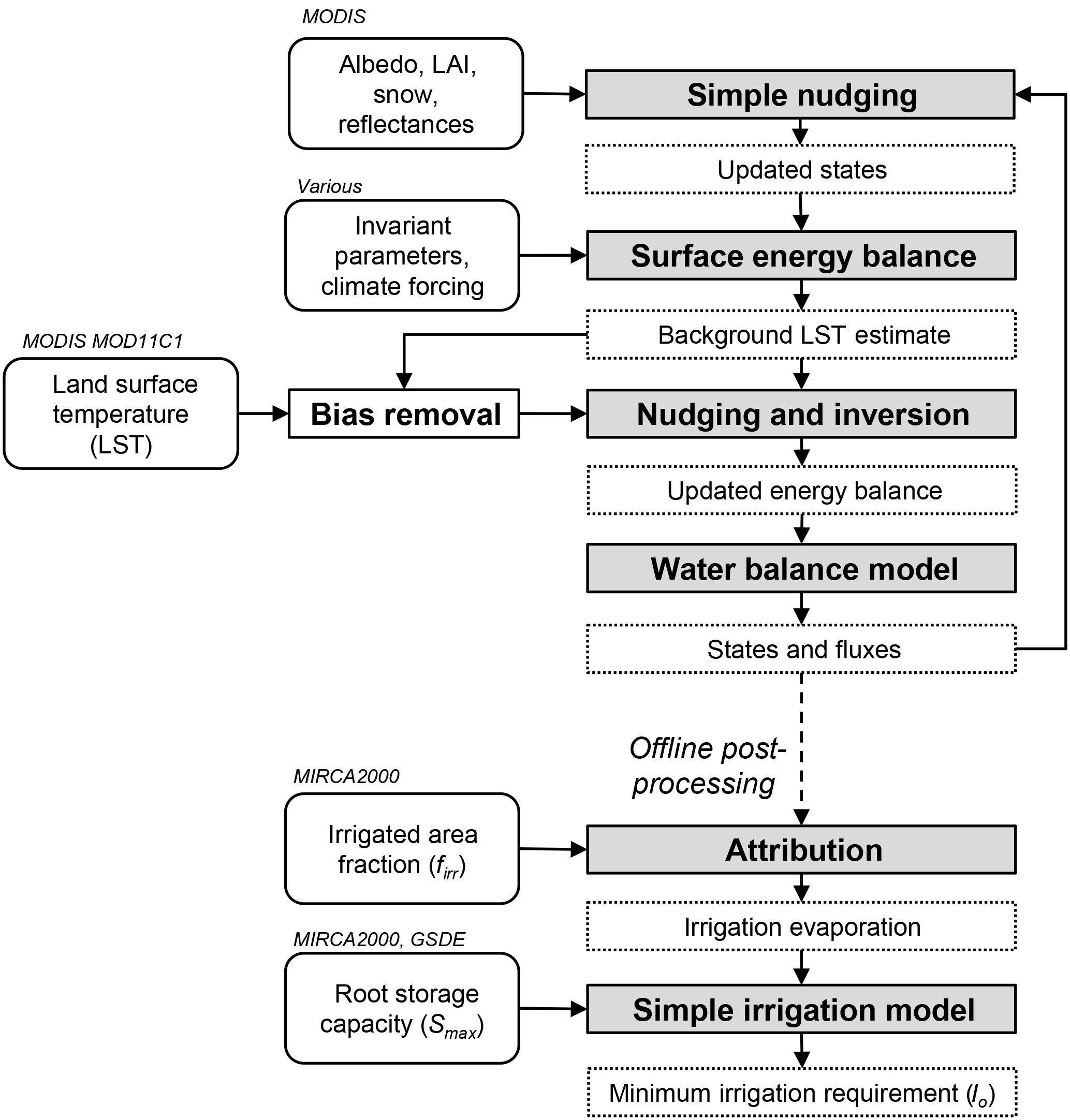
Figure 1 Illustration showing the processing steps and data used in each step. Acronyms relate to the input data that are described in the text.

2.1 Global water balance model description

The World-Wide Water model (W3) version 2 is an evolution of the AWRA-L and W3RA group of models. The AWRA-L model is used operationally for water balance estimation across Australia at 0.05^∘ resolution by the Bureau of Meteorology. An overview of the operational AWRA-L model (version 5) can be found in Frost et al. (2016b) with details on the scientific basis in Van Dijk (2010). Very briefly, the model operates at daily time step and is grid-based. Each cell is conceptualized to represent several parallel, small, identical catchments. The soil column is conceptualized as a three-layer unsaturated zone overlaying an unconfined groundwater store, from which capillary rise can occur. The unsaturated soil water balance and corresponding water and energy fluxes can be simulated separately for hydrological response units (HRUs) that each occupy a fraction of the grid cell. The surface energy and water balance is simulated using the Penman–Monteith model. The evaporative fluxes from transpiration, unsaturated soil, saturated soil and surface water are simulated subject to the overall constraint of potential evaporation E₀ within the same Penman–Monteith framework. Wet canopy evaporation is simulated outside this constraint for reasons described in Van Dijk et al. (2015), using a dynamic canopy version of the event-based Gash model (Van Dijk and Bruijnzeel, 2001; Wallace et al., 2013). Sub-grid parameterizations are applied to simulate the area fractions with surface water, groundwater saturation and root water access to groundwater dynamically, based on the hypsometric curves (i.e., the cumulative distribution function of elevation) for each grid cell (Peeters et al., 2013).

The W3 (version 2) model is a global implementation of AWRA-L (version 5) at the same 0.05^∘ resolution. Important differences are as follows. Separate HRUs were not considered, however the water balance of permanent waterbodies is calculated separately. Global gridded climate time series and surface, vegetation and soil parameterization data were used, including MSWEP v1.1 (Beck et al., 2017) precipitation estimates and other meteorological data from the WFDEI v1 dataset (Weedon et al., 2014). Monthly precipitation and air temperature climatology data at 30${}^{\prime \prime }$ from the WorldClim dataset (Hijmans et al., 2005) were resampled to 0.05 and 0.25^∘. Subsequently, the ratio and difference between the data at the finer and coarser resolution, respectively, were applied to the forcing data. Global datasets were also used to parameterize the distribution of different land surface types (Bicheron et al., 2008) and the properties of vegetation (Simard et al., 2011), soil (Shangguan et al., 2014) and aquifers (Gleeson et al., 2014; Beck et al., 2015). We used the cumulative distribution function of Height Above Nearest Drainage (HAND; Nobre et al., 2015) for each grid cell instead of hypsometric curves, which we derived from high-resolution global digital elevation models.

Five model parameters that were both relatively uncertain and influential were calibrated and regionalized by climate and land cover type class, using large global data sets of site measurements evaporation, near-surface soil moisture and a global dataset of catchment streamflow records (the parameters represent proportional adjustments to initial estimates of, respectively, maximum canopy conductance, relative canopy rainfall evaporation rate, soil evaporation, saturated soil conductivity and soil conductivity decay with depth). Differences less relevant here include the addition of a snow–water balance model with parameters from Beck et al. (2016) and grid-based river routing using a flow direction based on HydroSheds (Lehner et al., 2008) where available, and HYDRO 1k elsewhere. A range of W3-simulated water and energy balance terms has been made publicly available as part of “Tier-2” of the EartH2Observe project (Schellekens et al., 2017). The AWRA-L and W3 models have received extensive evaluation, demonstrating realistic estimates of evaporation, soil moisture, deep drainage, streamflow and total water storage (e.g., for more recent implementations, Tian et al., 2017; Frost et al., 2016a; Beck et al., 2016; Holgate et al., 2016).

The W3 model used here is not the only suitable modelling framework for the approach described. A similar method could be applied with other local or global models. The main requirements are that the model has a coupled water and energy balance model that simulates LST, and that it is amenable to data assimilation.

2.2 Data assimilation

All data assimilated here were derived from NASA's Moderate Resolution Imaging Spectroradiometer (MODIS) instruments. The data included albedo, reflectance, the leaf area index (LAI) and LST. We followed the following steps, except in the case of the LST. First, the MODIS band reflectances (product MCD43C4.005) were used to estimate the vegetation cover fraction and canopy conductance following Yebra et al. (2015, 2013). The surface water extent was estimated following Van Dijk et al. (2016). MODIS albedo (MCD43C3.005), the snow cover fraction (MCD43C4.005) and MODIS GLASS LAI product (Xiao et al., 2014) were used in their original form. Next, seven model states were updated using a simple nudging scheme. For each state, the observation and model error estimates were based on an assessment of the noise in the observational data, the expected dynamic rate of change and the expected skill of the model. The resulting “gain” factors (i.e., the relative weight of observations) varied from 0.5 for the LAI and snow fraction to 0.99 for surface water fraction (reflecting the low skill in the model to accurately predict surface water extent changes at 0.05^∘ resolution). The updated states were also used dynamically to update six related parameters of diagnostic model equations, including a parameter relating vegetation cover fraction to canopy conductance, another relating vegetation cover to LAI and four parameters relating the surface state to the albedo.

The approach to assimilate LST observations was different. In this case, the dynamic model was run one time step forward to produce a background estimate of the surface energy balance and evaporation flux. The corresponding average daytime LST (T_s, K) was estimated from the average daytime sensible heat flux (H, W m⁻²) as

$$\begin{array}{}\text{(1)}& T_{\text{s}}=T_{\text{a}}+{\displaystyle \frac{H}{{\mathit{\rho }}_{\text{a}}{c}_{\text{p}}{g}_{\text{a}},}}\end{array}$$

where T_a is air temperature (K), ρ_a air density (kg m⁻³), c_p specific heat capacity (J kg⁻¹ K⁻¹) and g_a(u) aerodynamic conductance (mm s⁻¹). The latter is a function of wind speed scaled by the wind speed measurement and vegetation height, respectively, following Thom (1975).

The poor characterization of spatial gradients in radiative exposure, air temperature and wind speed in areas with relief can cause a poor relationship between the observed and modelled LST (Kalma et al., 2008). Fortunately, secondary evaporation primarily occurs in regions with low relief. Therefore, data assimilation was only attempted for areas with an average slope of less than 3 % (calculated from the higher-resolution DEM). This threshold was empirically found to include a large majority of observed surface water inundation and mapped irrigation areas.

A second challenge relates to the inconsistency between the observation time-of-overpass LST and the model-predicted mean daytime LST. We assumed that the time-of-overpass and mean daytime LSTs will have different spatial averages but share a near-identical spatial pattern of deviations from the spatial averages. This assumption also helps to remove systematic bias, which is the largest source of error in the MODIS LST estimates used here (MOD11C1.006; Wan, 2015). Previous assessments report errors in MODIS that are within 0.7 K under conducive atmospheric conditions but can increase to 3 or 4 K due to errors in atmospheric correction that tend to cause a similar level of bias over a larger area (Wan et al., 2004; Wan, 2008; Wan and Li, 2008; Hulley et al., 2012).

In the assimilation step, first the median observed and the modelled LST were calculated for all low-relief grid cells within a spatial window of 15^∘ latitude and longitude and were subtracted from the respective gridded LST values to remove systematic bias. Subsequently, we calculated the difference between resulting observed and modelled LST values. The calculated difference was reduced by up to 1 K to conservatively allow for uncertainty in the assumptions and errors in the observations. Next, the model LST was updated with the remaining difference towards the MODIS-observed LST. An updated latent heat flux (λE^′ in W m⁻², the prime indicating the updated variable) can be calculated from an inverted version of the energy balance equation as

$$\begin{array}{}\text{(2)}& \mathit{\lambda }{E}^{\prime }=A-H^{\prime }=A-{\mathit{\rho }}_{\text{a}}{c}_p{g}_{\text{a}}\left(T_{\text{s}}^{\prime }-T_{\text{a}}\right)\end{array}$$

where A is available energy (W m⁻²). To ensure physical consistency within the model context, λE^′ was constrained to positive values below or equal to E₀. Temporal consistency was ensured by recording the ratio λE^′ ∕ λE and using it to adjust simulated λE for subsequent days until a new LST observation was available. Finally, E was calculated through division by the latent heat of vaporization λ. A fundamental assumption in this approach is that the partitioning between λE and H can be improved with information on LST but that the estimate of available energy A is correct.

To illustrate the data assimilation, a time series of observations and model results for a 0.05^∘ grid cell in the Nile delta in Egypt are shown in Fig. 2. This grid cell was chosen because it represents one of comparatively few grid cells worldwide deemed to be 100 % equipped for irrigation in global mapping (although the annual maximum NDVI derived from Landsat suggests that only 80 %–81 % of the area is in fact irrigated; see Fig. 2a). The processing steps are illustrated by a comparison of observed, background and analysis LST estimates for the year 2002 (Fig. 2b), the resulting sensible heat flux (Fig. 2c) and daily evaporation (Fig. 2d). Corresponding temporal patterns in the evaporative fraction (E ∕ E₀) show that data assimilation brings the temporal pattern of the evaporative fraction in close agreement with the satellite-observed vegetation cover fraction (Fig. 2e), which provides a largely independent consistency test.

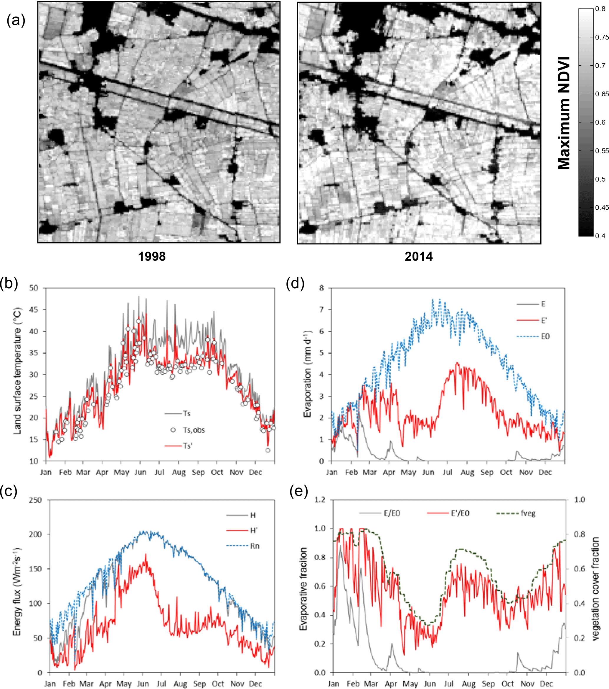
Figure 2 Illustration of method to assimilate MODIS land surface temperature observations. Data shown are for 2002, for a 0.05^∘ grid cell in the Nile River delta, Egypt (centred 31.075^∘ N, 30.325^∘ E) and panels represent the following: (a) Maximum normalized difference vegetation index (NDVI) derived from Landsat imagery provided by Google Earth Engine, suggesting that effectively 81 % and 80 % of the grid cell was cropped in 1998 and 2014, respectively; (b) Land surface temperature, with background (T_s, grey line), observed (T_s,obs, circles) and analysis ($T_{\text{s}}^{\prime }$, red line) estimates for the grid cell with average bias across the 15^∘ window removed; (c) Sensible heat flux, with background (H, grey) and analysis (H^′, red) estimates along with net radiation (R_n, blue); (d) Evaporation, with background (E, grey) and analysis (E^′, red) estimates and potential evaporation (E₀, blue) and (e) Evaporative fraction, with background (E ∕ E₀, grey) and analysis (E^′ ∕ E₀, red) and, for comparison, vegetation cover fraction derived from MODIS NDVI (f_veg, green).

2.3 Irrigation water use estimation

For irrigated areas, the long-term average difference between precipitation and total evaporation derived from data assimilation provides an estimate of the importance of additional water inputs. However, it cannot be interpreted directly as an estimate of irrigation water requirements, much less as an estimate of water withdrawals. This is because precipitation and crop water requirements are both unevenly distributed in time, and there is limited water storage capacity in the crop root zone. Additional water is lost from the root zone through drainage and runoff, which will need to be compensated by additional irrigation inputs. This field-level irrigation inefficiency does not necessarily change the long-term net water balance, since provided that total precipitation and evaporation do not change, the additional inputs will equal the additional runoff and drainage. However, such inefficiencies do need to be accounted for when estimating the total amount of irrigation water required (Siebert and Döll, 2010).

The estimation of total field-level irrigation water requirements is sensitive to assumptions about the capacity for added water to remain stored in the root zone and about irrigation strategies (e.g., pursuing a stable low or high soil moisture or paddy water level, suboptimal or soil moisture deficit irrigation, flood irrigation or partial drip irrigation and so on). Here, we estimated a minimum field-level irrigation requirement (I₀ in mm), which can be taken as a conservatively low estimate of irrigation that represents highly efficient irrigation practices. The estimation of I₀ was done after and entirely separate from the data assimilation process. Therefore, what follows had no bearing on the estimation of secondary evaporation.

We used global mapping by crop type to estimate I₀ using a plausible range of published assumptions about water storage capacity. It was assumed that irrigation is just sufficient to replenish lost water without any direct drainage or runoff losses. That is, losses only occur when precipitation exceeds available storage capacity. Following Siebert and Döll (2010), we estimate the available root zone storage capacity (S_max in mm) for the irrigated crop type N=1.26 from the estimated harvested area (A_i in ha) of each as contained in the MIRCA2000 dataset (Portmann et al., 2010). These numbers are combined with assumed rooting depth (z_i) and the allowable fraction depletion of available soil water p_i (Allen et al., 1998) for each crop type as proposed by Siebert and Döll (2010). The plant available water content (θ_a) was estimated using global soil property data (Shangguan et al., 2014), calculated as the difference between θ at field capacity and the permanent wilting point assumed to correspond to water potential values of −3.3 and −150 m, respectively. This is represented by the procedure

$$\begin{array}{}\text{(3)}& S_{\text{max}}={\displaystyle \frac{\sum A_i{z}_i{p}_i}{\sum A_i}}{\mathit{\theta }}_{\text{a}}{f}_{\text{irr}},\end{array}$$

where f_irr is the fraction of the grid cell area that is equipped for irrigation (Portmann et al., 2010). This method produced a global average root zone storage of 51 mm per unit of irrigated land, with 90 % of values between 10–85 mm and values depending primarily on the value of z_i.

Because we have observation-based estimates of evaporation, we do not simulate the influence of soil water status on evaporation. Instead, we propagate a simple water balance model forced with evaporation estimates. In other words, the change in soil moisture storage from one day (S_t) to the next (S_t+1) is the net result of gross rainfall onto the irrigated area (P_irr), evaporation from the irrigated area (E_irr), the minimum irrigation water application required (I₀) and drainage (D), with storage and cumulative daily fluxes in mm. This is represented by the equation

$$\begin{array}{}\text{(4a)}& S_{t+\mathrm{1}}=S_t+P_{\text{irr}}-E_{\text{irr}}+I_{\mathrm{0}}-D.\end{array}$$

Partial rainfall (P_irr) is proportional to the irrigation fraction and grid cell rainfall (P), such that

$$\begin{array}{}\text{(4b)}& P_{\text{irr}}=f_{\text{irr}}P.\end{array}$$

It is assumed that any increase in the estimate of evaporation ($E^{\prime }-E)$ from data assimilation is due to irrigation, where this occurs. Therefore, E_irr is given by

$$\begin{array}{}\text{(4c)}& E_{\text{irr}}=f_{\text{irr}}E+\left(E^{\prime }-E\right).\end{array}$$

Any soil water additions exceeding the maximum storage capacity (S_max) are assumed to become drainage, and irrigation is assumed to be just enough to prevent S<0, such that

$$\begin{array}{}\text{(4d)}& I_{\mathrm{0}}=max\left(E_t-P_{\text{irr}}-S_t,\mathrm{0}\right);\end{array}$$

$$\begin{array}{}\text{(4e)}& D=max\left(S_t+P_{\text{irr}}-E_t-S_{max},\mathrm{0}\right).\end{array}$$

Rainfall interception losses are included in E. Surface runoff and residual drainage are assumed negligible when S<S_max. This is an important simplification but is consistent with the definition of a minimum irrigation requirement estimate that reflects optimal efficiency. The daily water balance model was evaluated with an initial state of S=S_max and propagated from 2000 to 2014. The first year was not used in subsequent calculations to allow for artefacts from the initial state chosen.

2.4 Evaluation of basin water balance

One test of the accuracy of secondary evaporation estimates is to evaluate whether their inclusion in the basin water balance improves agreement with observations. The difference between the E^′ derived from data assimilation and the background estimate E is interpreted to be derived from lateral inflows and can be represented by

$$\begin{array}{}\text{(5a)}& E_{\text{lat}}=E^{\prime }-E.\end{array}$$

For any basin, the total net amount of discharge from the basin (Q_n) is the result of the gross amount of streamflow generated in all tributaries (Q_g) minus secondary evaporation of flows downstream (E_lat) and the change in storage derived from those flows (ΔS_lat), represented by

$$\begin{array}{}\text{(5b)}& Q_{\text{n}}=Q_{\text{g}}-E_{\text{lat}}-\mathrm{\Delta }{S}_{\text{lat}}.\end{array}$$

Natural storage variations in soil and groundwater and river channel storage are explicitly simulated by the model and are not included in ΔS_lat. Storage changes in other surface waterbodies (e.g., lakes and reservoirs), river–groundwater exchanges and induced soil or groundwater storage changes directly related to inundation or irrigation (including pumping) would affect ΔS_lat. It is assumed here that the magnitude of ΔS_lat is negligible compared to the other terms if fluxes are averaged over the period 2001–2014. This needs to be considered when interpreting results for individual basins.

We used discharge data for large basins to evaluate whether our estimates of E_lat improved the overall agreement between the modelled and observed Q_n. The river discharge data used were drawn from the global database of end-of-river discharge records compiled by Dai et al. (2009). This includes data for 925 rivers worldwide. Out of these, we considered only basins for which more than five years of data were available during 1995–2014. This longer period was adopted because few basins had sufficient measurements after 2000. To avoid errors arising from differences in the delineation of basins, we rejected basins with a catchment area of less than 100 000 km² and those with a reported drainage area that was more than 25 % different from the DEM-derived basin area at the river mouth. For the remaining 38 large basins the temporal and area-average discharge was calculated and compared to the modelled Q_n and Q_g (all in mm yr⁻¹).

Closed or endorheic basins represent a special case where Q_n=0 and can also be used to construct a water balance. The 0.05^∘ flow direction grid was used to delineate all internally draining basins located between 72^∘ N and 60^∘ S (further towards the poles, the DEM is affected by land ice). Adjoining endorheic basins were merged into contiguous regions to avoid incorrect basin delineation. From the resulting regions, all those with a surface area greater than 50 000 km² were extracted, resulting in 13 contiguous regions. For these regions, Eq. (5b) was evaluated and compared to the expected Q_n=0.

The LST data assimilation changes evaporation without adjusting other water balance terms and hence does not conserve mass balance. In both open and closed basins, this can produce a positive or negative Q_n from Eq. (5b). A difference between the estimated and observed Q_n can occur for four reasons; Q_g is underestimated, E_lat overestimated, ΔS_lat is non-negligible or (for discharging basins only) the recorded Q_n is in error.

2.5 Evaluation of apparent irrigation water use

Evaluating estimates of secondary evaporation due to irrigation is challenging. Direct observations of evaporation from irrigated land are not widely available, represent point observations and include primary evaporation. At the basin or country level, estimates of irrigation water use can be categorized as “bottom-up” or “top-down” estimates. Bottom-up estimates require the scaling of the estimated crop water use to field-level irrigation requirements. Top-down estimates involve estimating large-scale withdrawals (e.g., by the differencing of discharge measurements along a river reach or measured bulk diversions) and accounting for “project” or scheme losses along the distribution network (Bos and Nugteren, 1990). Both approaches have large uncertainties but provide estimates of the order of magnitude of irrigation water use.

Bottom-up estimates of irrigation water use at the global scale and for individual countries are available from previous studies (Siebert et al., 2010; Wada et al., 2014; Siebert and Döll, 2010). They involve soil-vegetation water balance modelling. Similar to the approach used here, these methods require assumptions about root zone storage capacity, the rate of drainage of water from the root zone, the permissible range of root zone soil moisture and the efficiency of irrigation. Unlike the approach used here, they furthermore require assumptions about evaporation, usually following FAO's crop factor approach (Allen et al., 1998) to model crop water use. The resulting one-dimensional irrigation water requirement estimates are subsequently extrapolated spatially with mapping of areas equipped for irrigation (e.g., Portmann et al., 2010), using assumptions about the number of crop rotations and the area factually irrigated. Each of these assumptions introduces errors and uncertainties. Nonetheless, a comparison with these studies should provide insight into the method developed here.

An important source of uncertainty in our estimation of the large-scale I₀ is due to the diffuse spatial distribution of irrigated areas, which is further amplified in current mapping products. The mapping of areas equipped for irrigation contained in the MIRCA2000 dataset (Portmann et al., 2010) was done at 0.08^∘ grid resolution and linearly interpolated to 0.05^∘ resolution in this study. Even at this high resolution, a large proportion of total irrigable land occupies only a small fraction of a grid cell (Fig. 3).

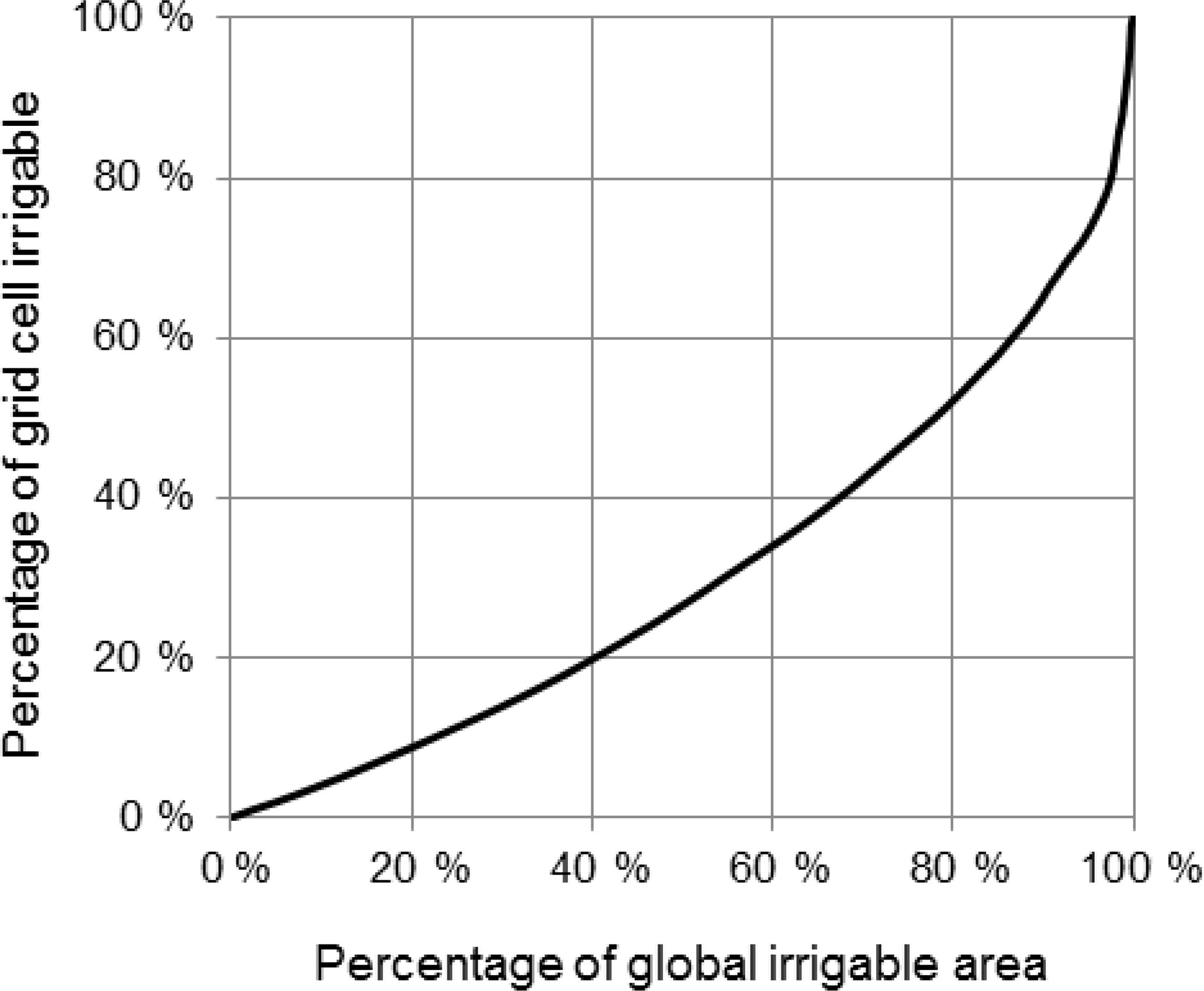
Figure 3 Cumulative distribution curve or quantile plot describing the degree to which the global irrigable area is concentrated. It shows that at 0.05^∘ grid resolution, almost half of the total global irrigable area occupies less than 25 % of a grid cell.

The degree of concentration differs between countries for two reasons. Firstly, the true distribution of irrigation land varies. For example, irrigation tends to be concentrated in large surface water irrigation schemes (e.g., the Nile delta and Indus floodplains) but can be highly distributed where supplementary irrigation water is drawn from unregulated streams or groundwater. Secondly, the quality, resolution and predictive value of information related to irrigation area varies widely, which affects the accuracy of mapping (Portmann et al., 2010). The distribution of irrigation land introduces uncertainty in the attribution of E^′ in grid cells of small fractions of irrigated land. We expect that the fraction of a grid cell that needs to be irrigated to create a measurable LST signal may be around 10 % but will vary spatially depending on the LST contrast between irrigated and non-irrigated land. To account for this uncertainty, we calculated the mean I₀ (Eq. 4) per unit irrigation area for all grid cells with more than 1, 2, 5, 10 and 25 % of the area equipped for irrigation. These estimates were subsequently multiplied with the total area equipped for irrigation in each country. The coefficients of variation among the five estimates was calculated as a measure of estimation uncertainty.

The AQUASTAT database (FAO, 2017) provides country-level estimates of agricultural water withdrawal (W in km³ yr⁻¹) from the surface and groundwater. (Domestic and industrial withdrawals are not considered because a large fraction of these withdrawals is not evaporated but returned to the environment.) The estimates are derived by different methods for different countries and likely include both bottom-up and top-down techniques. Estimates also relate to different periods or years. Despite these uncertainties, they currently represent official international statistics for each country. Any comparison of field-level irrigation water application (I₀) and large-scale water withdrawal (W) needs to account for inefficiencies in the entire water distribution network, both on- and off-farm. These include evaporation, leakage and return flow. `Project efficiencies' that express the ratio of I<sub>0</sub> over W can be estimated in principle, but this requires detailed ancillary data (Bos and Nugteren, 1990). In their global modelling study, Siebert and Döll (2010) proposed ratios range from 0.25 for irrigation dominated by paddy rice to 0.70 for efficient crop irrigation methods in Canada, Northern Africa and Oceania. We did not assume values but instead calculated an `apparent' bulk project efficiency for each country, by dividing the ratio of the modelled I₀ over W reported in AQUASTAT. The plausibility of the resulting values was subsequently interpreted within the framework developed by Bos and Nugteren (1990).

2.6 Secondary evaporation and the global water cycle

Total secondary evaporation was estimated as the sum of open water evaporation plus the difference $E^{\prime }-E$ , representing the difference between the modelled primary evaporation E for a situation where precipitation is the only source of water (the background estimate) and the total evaporation E^′ resulting from LST assimilation (the analysis estimate). The resulting estimate of total secondary evaporation is a hypothetical, model-based quantity. Evaporation in the absence of lateral flows is counterfactual and not necessarily accurately estimated by the model, particularly in humid environments. Furthermore, all open water evaporation was included in secondary evaporation; we did not attempt to estimate the evaporation that might have occurred from the surface had it not been covered by water.

The difference $E^{\prime }-E$ was distributed dynamically in proportion to the magnitude of each of three evaporation terms (i.e., transpiration, soil evaporation and open water evaporation; wet canopy evaporation was left unchanged). A component of secondary evaporation was attributed to irrigation following the method described earlier. The remainder could be attributed to permanent waterbodies, ephemeral waterbodies and a residual component that includes any evaporation from replenished wetlands and floodplains as well as any use of groundwater sources beyond those simulated by the model to occur from shallow groundwater (Peeters et al., 2013).

3 Results

3.1 Basin water balance

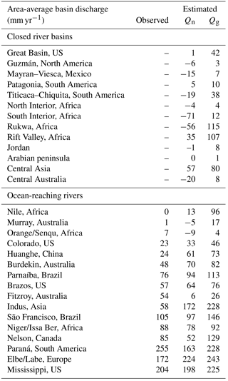
The combined surface area of the 51 basins used in evaluation (38 ocean-draining and 13 closed basins) was 63 million km² or 47 % of the ice-free land surface area (Fig. 4). For each region, the period-average measured discharge (zero in the case of closed basins) was compared with the modelled Q_g and Q_n (Fig. 5, Table 1). Overall, accounting for secondary evaporation produced a very small improvement in the correlation between observed and estimated discharge (Fig. 5a, b). However, the largest error contribution was from basins with high discharge rates, where secondary evaporation represents a small fraction of Q_g. A clearer improvement in the agreement was found for basins with less than 300 mm yr⁻¹ net discharge (Fig. 5c, d). The explained variance (R²) increased from 0.67 to 0.71, and there was a reduction of the bias from +38 to +2 mm yr⁻¹. Water balance estimates were improved considerably for several basins, including the Indus river (“I” in Fig. 5c, d), Nile river, the Great Basin in the USA and the African Rift valley (Table 1). The agreement could not improve where Q_g estimates were already lower than observed, such as the Paraná and Fitzroy Rivers (“P” and “F” in Fig. 5c, d). Water balance estimates for some closed basins were also degraded, evident from negative Q_n values (e.g., the South Interior and Rukwa basins in southern Africa), implying that Q_g was underestimated, secondary evaporation overestimated, or both (Table 1).

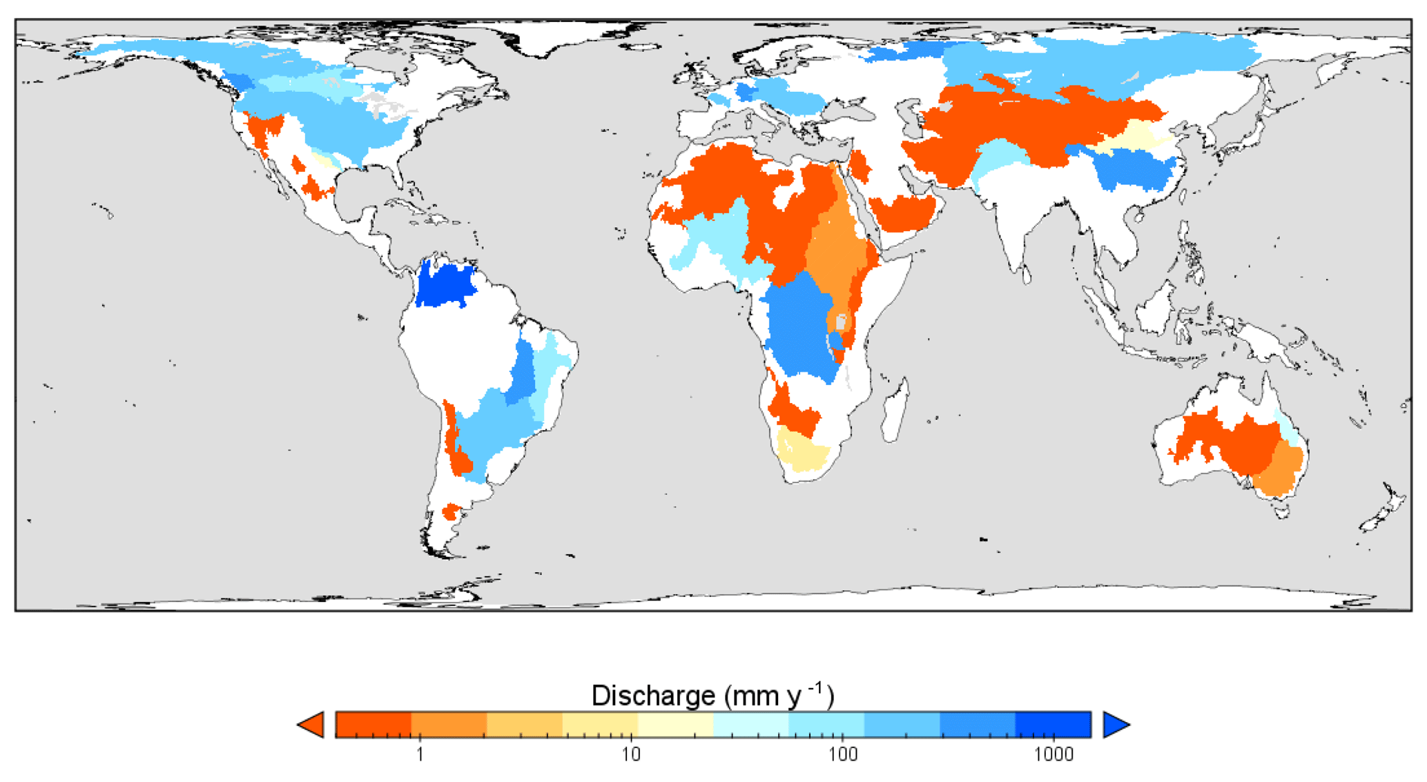
Figure 4 Extent and area-average annual discharge for the 38 ocean-draining (orange to blue) and 13 closed basins (dark orange) used in the evaluation. The two darkest blue colours indicate a discharge in excess of 300 mm yr⁻¹.

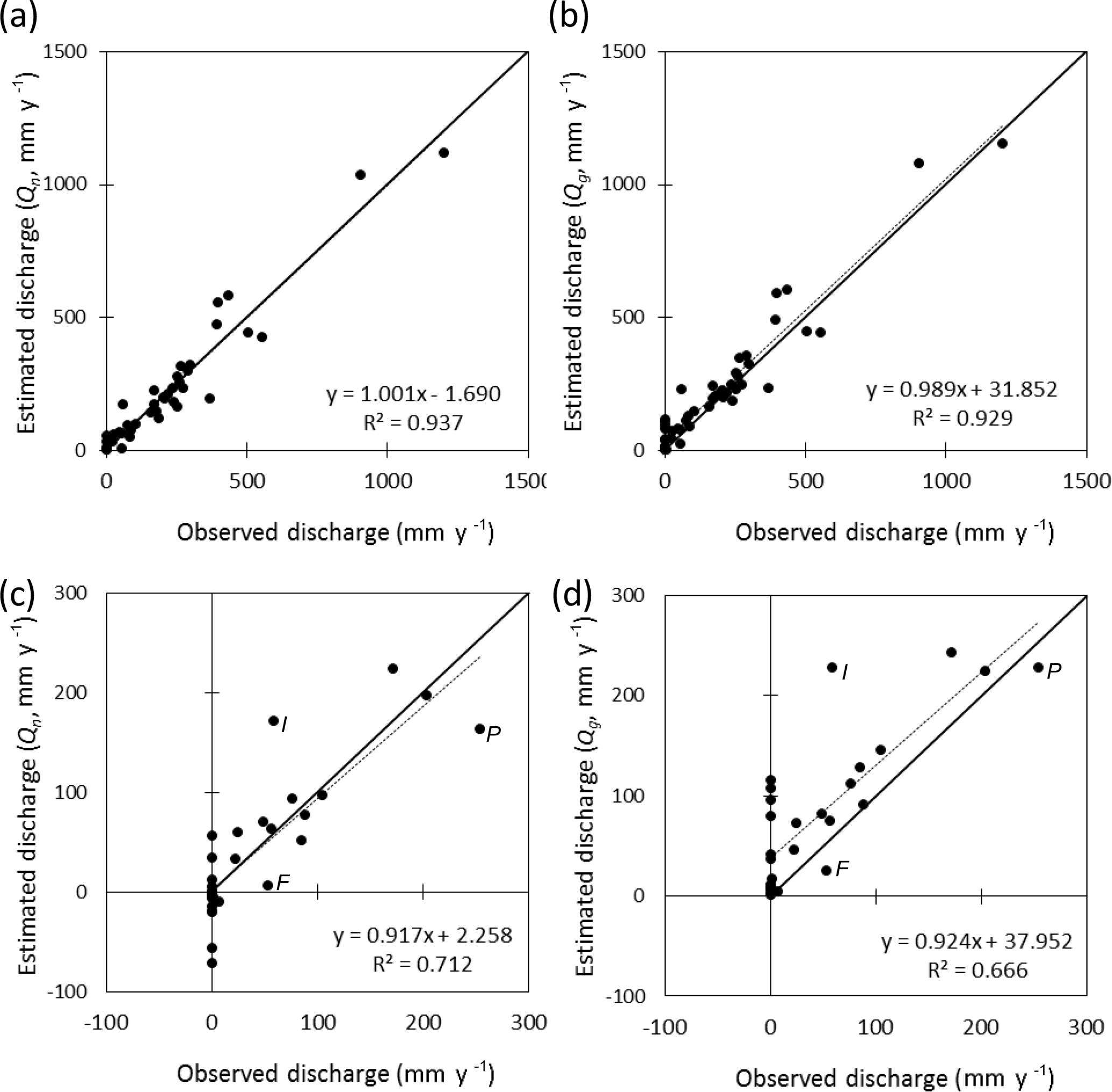
Figure 5 Comparison of observed basin-average discharge (mm yr⁻¹) for large basins that are internally draining (i.e., zero discharge) or have adequate station discharge data, respectively, with model estimates of (a) net discharge (Q_n), that is, gross discharge (Q_g) minus secondary evaporation and (b) Q_g only. Panels (c) and (d) represent data for discharge below 300 mm yr⁻¹ only (cf. Table 1). Letters indicate the Indus (I), Paraná (P) and Fitzroy (F) River.

Table 1 Area-average discharge (mm yr⁻¹) for selected basins as observed and estimated by the model in the presence (Q_n) and absence (Q_g) of secondary evaporation, respectively. Listed data for basins with discharge less than 300 mm yr⁻¹ only (cf. Fig. 5c, d).

3.2 Irrigation water requirements

Spatiotemporal estimates of I₀ at 0.05^∘ and daily time step were aggregated to country-level estimates in km³ yr⁻¹ (Table 2). Also calculated were the coefficient of variation in I₀ estimates (CV${}_{I_{\mathrm{0}}})$ caused by the treatment of “mixed pixels” in irrigation mapping, FAO-reported annual W and the apparent project irrigation efficiency. Global I₀ for 2001–2014 was 680 km³ yr⁻¹ (standard deviation 110 km³ yr⁻¹). This value is lower than estimates of contemporary irrigation water use reported in the literature of 1092 km³ yr⁻¹ (Döll and Siebert, 2002), 1180 km³ yr⁻¹ (Siebert and Döll, 2010) and 994–1179 km³ yr⁻¹ (Wada et al., 2014). Estimates of I₀ listed for seven countries by Döll and Siebert (2002) were all higher than those found here (Table 2) and even more than double for the USA (112 vs. 48 km³ yr⁻¹) and Spain (21 vs. 5.1 km³ yr⁻¹). Quoted independent estimates were 113 km³ yr⁻¹ for the USA (Solley et al., 1998) and 15 km³ yr⁻¹ for Spain (J. A. Ortiz cited in Döll and Siebert, 2002).

Table 2 Irrigation water withdrawal (W) as reported to FAO for the 20 countries with largest agricultural withdrawals, along with the estimated minimum field-level irrigation requirement (I₀), the coefficient of variation in I₀ estimates (CV${}_{I_{\mathrm{0}}})$ and the apparent project efficiency (I₀ ∕ W).

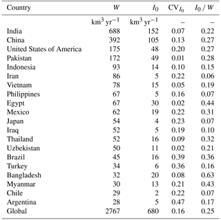
Figure 6 Comparison of country-level agricultural water withdrawal (W) (FAO, 2017) and estimated minimum irrigation requirement (I₀) expressed as (a) total volume and (b) depth per unit area of area equipped for irrigation for countries with >1 km³ yr⁻¹ withdrawals (N=91). Dotted lines show apparent project efficiencies between the two quantities. Countries indicated in (a) are Egypt (EG), Pakistan (PK), United States (US), China (CN) and India (IN), and in (b) Cambodia (KH), Senegal (SN), Mauritania (MR), United Arab Emirates (AE), Chile (CL) and the Philippines (PH).

The I₀ explains 96 % of the variance in W by country (Fig. 6a), but total variance is dominated by only four countries, and the area equipped for irrigation explains already explains 86 % of the variance. Volumes were divided by the total area equipped for irrigation to normalize for these effects. The normalized I₀ explained 38 % of the variance in the normalized W (Fig. 6b). A high correlation between the two is not necessarily to be expected, as country-average project efficiencies will vary (represented by the lines in Fig. 6b). For example, a low efficiency is inferred and would be expected in the Philippines, where irrigation is dominated by paddy rice agriculture, whereas higher efficiencies would be expected in large schemes in arid countries such as Egypt and Mauritania. Nonetheless, apparent efficiencies are generally lower than would be expected based on benchmark estimates provided by Bos and Nugteren (1990). For example, using global volumes of I₀ and W, a project efficiency of 0.25 is calculated. This is lower than estimates of 0.36–0.43 assumed in previous studies (Döll and Siebert, 2002; Wada et al., 2014; Siebert and Döll, 2010). Physically impossible or implausible project efficiencies were also calculated for some countries, including Cambodia (I₀ ∕ W>1) and the United Arab Emirates and Chile (I₀ ∕ W<0.1) (Fig. 6b). Possible explanations for this will be discussed.

3.3 Secondary evaporation and the global water cycle

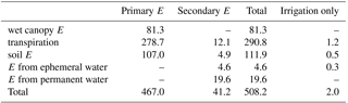
We estimate that secondary evaporation contributed 41.2 mm yr⁻¹ or 8.1 % to the total evaporation from the global land area during 2001–2014 (Table 3), equivalent to 5.4 % of terrestrial precipitation (759 mm yr⁻¹) and 16 % of generated streamflow (258 mm yr⁻¹). Globally, only a very small percentage of all secondary evaporation (5 %) was due to irrigation. Overall more important pathways for secondary evaporation were evaporation from permanent waterbodies (48 %), enhanced transpiration associated with wetland vegetation or greater-than-predicted groundwater uptake (27 %), soil evaporation (11 %) and evaporation from ephemeral waterbodies (10 %). Surface and groundwater inputs enhance global plant transpiration by an estimated 12.1 mm yr⁻¹, representing a 4.4 % increase. Of this increase, 10 % can be attributed to irrigation.

Table 3 Estimates of annual primary and secondary evaporation (E in mm yr⁻¹) components for 2001–2014 expressed as water depths across the global terrestrial area (149×10⁶ km²).

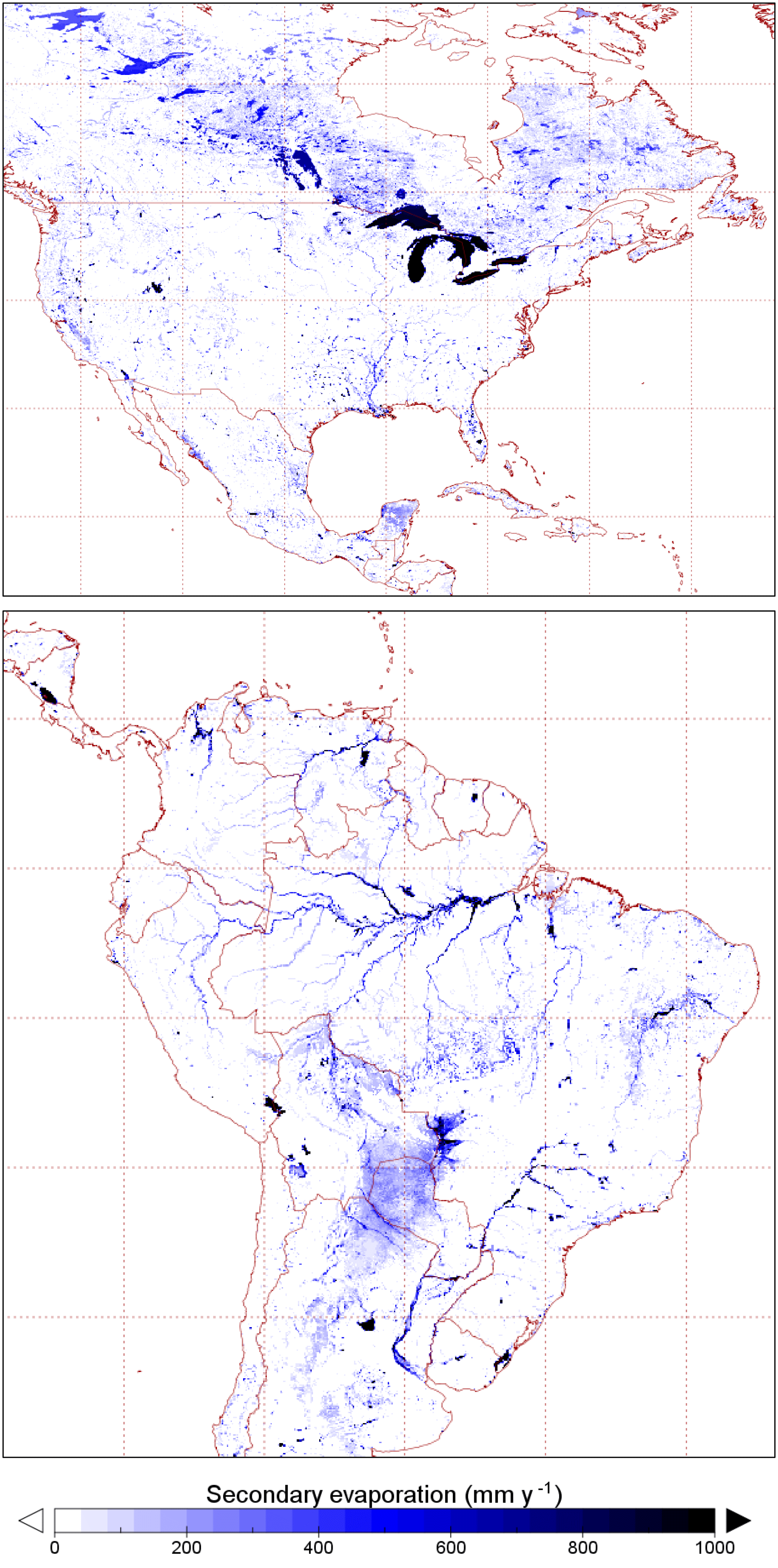
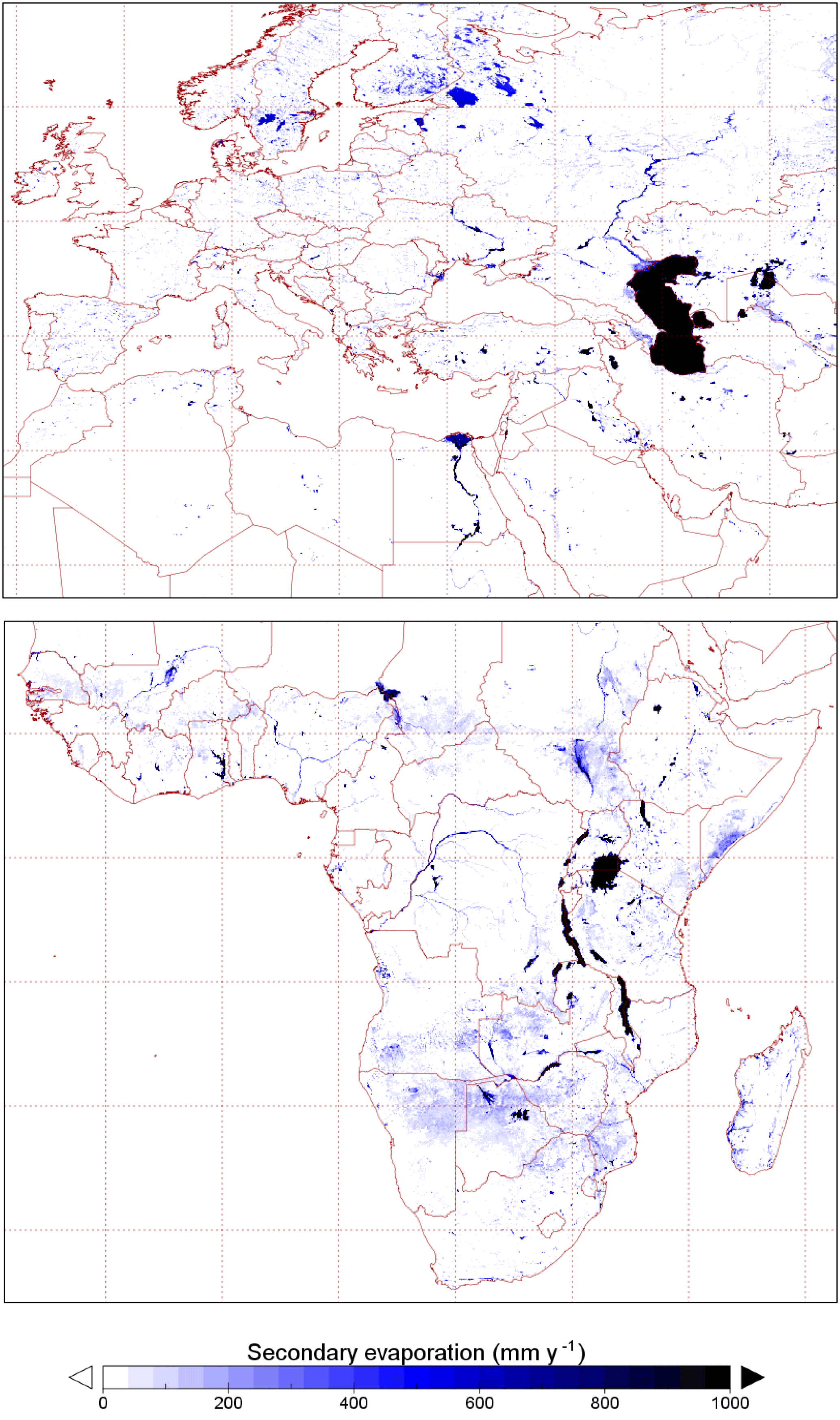
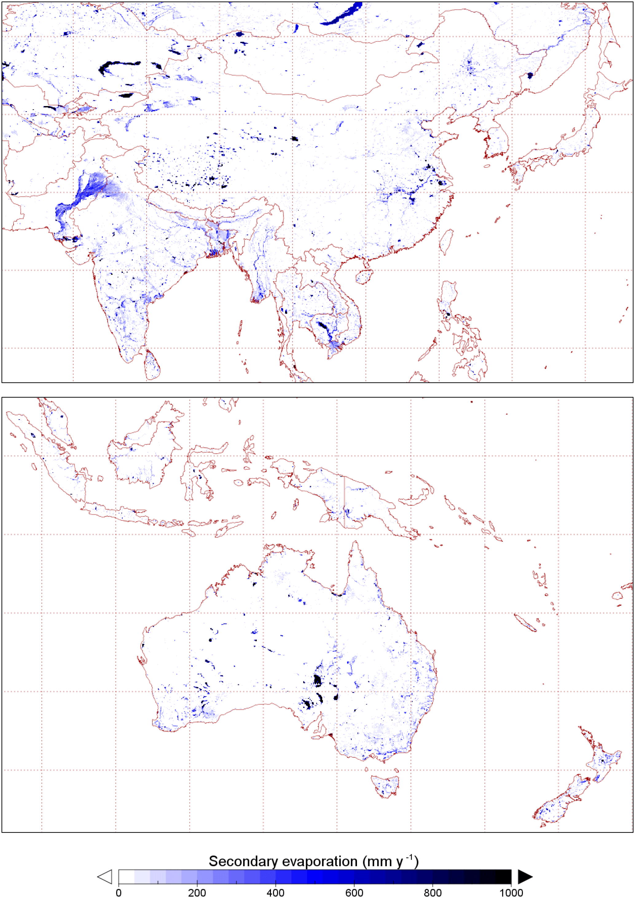
The spatial distribution of evaporation from irrigation areas (Fig. 7a) and permanent waterbodies (Fig. 7b) largely reflects the irrigation and water mapping input data, respectively. The spatial distribution of other sources of secondary evaporation provides some new insights (Fig. 7c). Globally, some areas with the greatest secondary evaporation volumes include receiving floodplains in tropical monsoonal regions. The main regions in South America include the Gran Chaco and Pantanal plains and the Amazon floodplains (Fig. 8). The main regions in Africa the Southern Interior basin in Botswana and surrounding countries (including the Okavango delta and other wetlands) and the floodplains of the White Nile river in South Sudan and the Inner Niger delta (Fig. 9). Other areas with high secondary evaporation rates include the Yucatán peninsula in Mexico (Fig. 8), the boreal wetlands and ephemeral lakes of Canada and Scandinavia (Figs. 8 and 9, respectively) and the salt lakes and floodplains of inland Australia (Fig. 10).

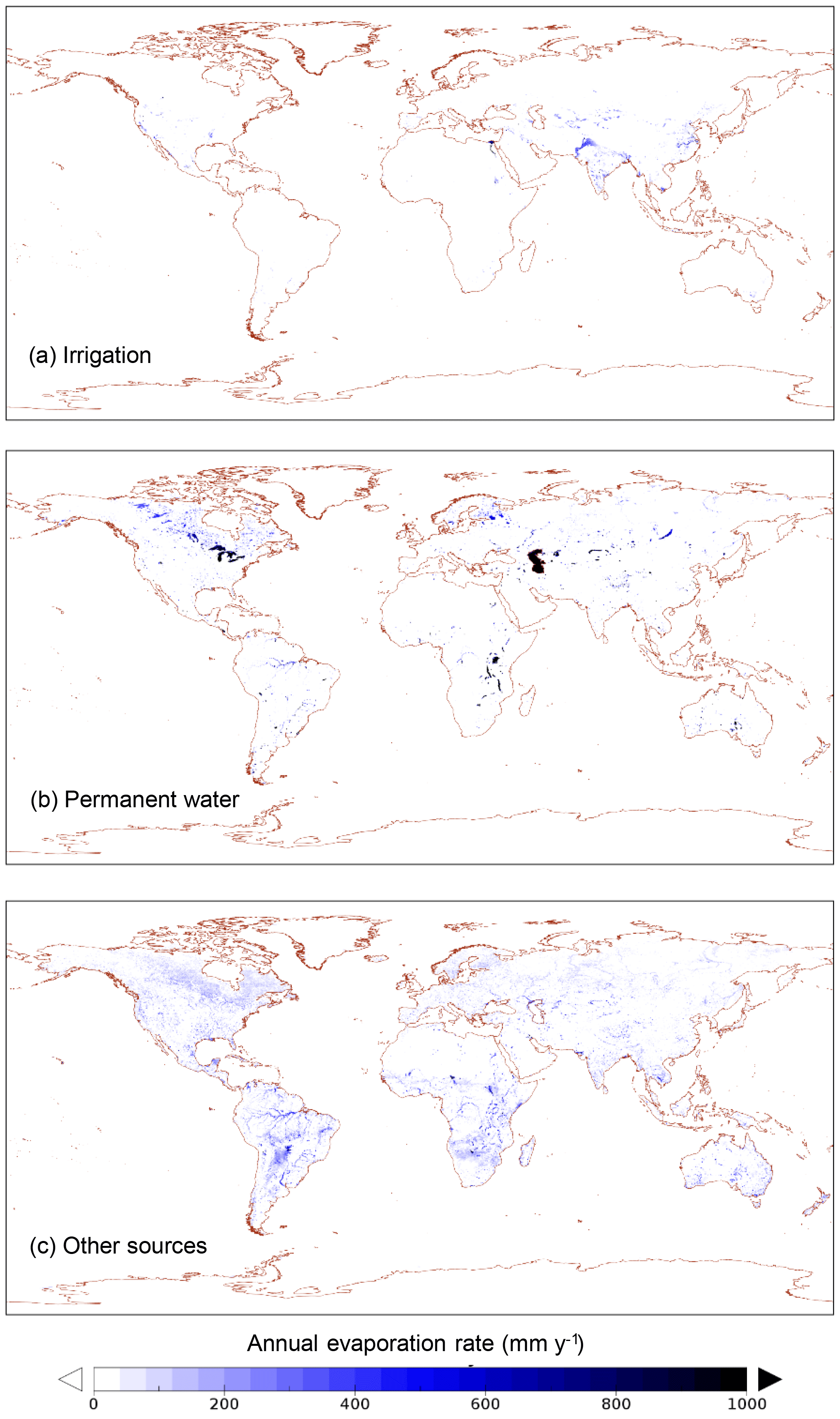
Figure 7 Spatial distribution of estimated secondary evaporation losses derived from (a) irrigation, (b) permanent waterbodies and (c) other sources, including wetlands and floodplains.

Figure 8 Spatial distribution of secondary evaporation losses in the Americas.

Figure 9 Spatial distribution of secondary evaporation losses in Eurasia and Africa.

Figure 10 Spatial distribution of secondary evaporation losses in eastern Asia and Oceania.

There is a pronounced seasonal cycle in secondary evaporation at the global scale (Fig. 11). The rate of secondary evaporation is more than 2 times higher in the northern summer than in northern winter. This is primarily due to the greater rate of evaporation from the many surface waterbodies in formerly glaciated regions, including the American Great Lakes, as well as a higher rate of evaporation from the Caspian Sea. By contrast, secondary evaporation in regions located wholly or partially in the Southern Hemisphere show a much less pronounced seasonal cycle and a greater influence of water availability. Averaged over time, each of the regions considered makes a similarly sized contribution to secondary evaporation globally (10 %–24 %) with the exception of Antarctica (0.4 %).

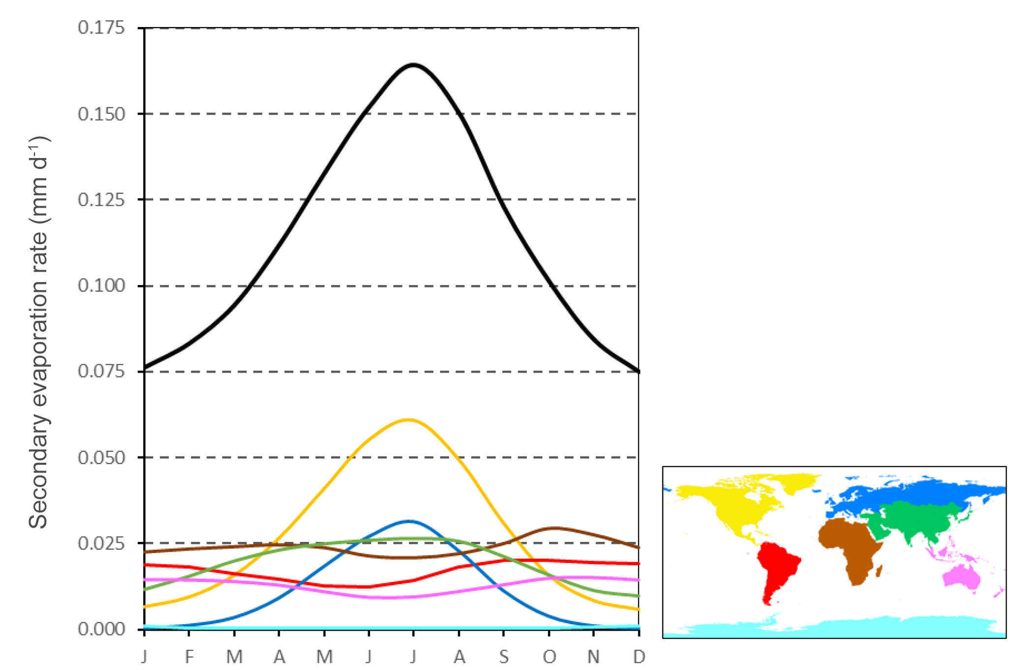
Figure 11 Average (2001–2012) seasonal cycle of secondary evaporation at the global scale (black line) and the contribution from different regions (colours corresponding to the map). All rates are expressed in mm d⁻¹ for the global land area.

4 Discussion

4.1 Uncertainties in evaporation estimation

The uncertainty in estimates of secondary evaporation arises from three main sources: (1) estimation of “background” evaporation E; (2) estimation of surface water evaporation; and (3) estimation of total evaporation E^′ by LST assimilation. A formal assessment of error in each of these terms is not possible for lack of observations and will vary in space and time. Below we discuss what we expect to be the main sources of uncertainty in each component.

An error in background model E may be compensated by data assimilation, but still leads to an error in the estimated secondary evaporation, calculated as $E^{\prime }-E$. The main sources of error in E vary as a function of environmental conditions and the quality and density of the measurements on which the meteorological forcing data are based. In water-limited environments, the most likely sources of error in E are errors in precipitation estimates and the simulation of water availability in the root zone. The quality of precipitation estimates is relatively poor in many of the world's dry regions (Beck et al., 2017). Information on the ability of vegetation to access deeper soil moisture and groundwater is important, particularly in ephemerally wet systems, but is not available at the global scale. In humid environments, the most likely sources of error in E are in the estimation of rainfall interception losses, the net available energy for evaporation and surface conductance. As part of earlier model development, background E was compared with estimates derived from flux tower observations and compared with alternative ET estimation methods (Yebra et al., 2013; and supplement to this article). These evaluations showed no systematic bias in E and a standard difference of 135–168 mm yr⁻¹ across sites. This total difference also includes errors in the flux tower-derived estimates (e.g., due to a lack of energy balance closure) and differences arising because the tower footprint is not representative of the grid cell.

Observation-based estimates of large-area evaporation (i.e., $>\mathrm{0.05}{}^{\circ }$) from waterbodies, wetlands and irrigated areas are scarce. Some site measurements of wetland and irrigation evaporation have been published (e.g., Guerschman et al., 2009) but typically reflect an environment with very high spatial variation and therefore often cannot easily be compared to estimates at 0.05^∘. A coordinated effort that collates observations of secondary evaporation and combines these with historical time series remote sensing imagery (cf. Fig. 1a) to generate estimates at a more representative spatial scale would appear necessary and valuable.

Errors in the estimation of surface water evaporation are the combined result of errors in the estimation of open water evaporation rate and the mapping of surface water extent. Open water evaporation rate was estimated using the Priestley and Taylor (1972) approach. An important uncertainty in this approach is that it does not account for strong contrasts in near-surface water temperatures. The surface water extent was mapped using 8-day MODIS shortwave infrared (SWIR) reflectance composites (Van Dijk et al., 2016). Systematic overestimation of water extent can occur in low-relief regions with very low SWIR reflectance (e.g., lava fields), whereas underestimation can occur in regions with a dense elevated canopy that prevents water detection (e.g., floodplain forests or mature flooded crops). Values of the updated λE^′ were constrained to positive values below or equal to potential evaporation E₀. Therefore, any gross underestimation of E₀ by the model due to errors in meteorological forcing data would have resulted in an underestimation of the true evaporation rate.

The LST assimilation mitigates estimation errors in background and open water evaporation but is also subject to uncertainties of its own. The technique developed here relies on the assumption that there is a perfect correlation between spatial LST anomalies at the time-of-overpass (around 10:00 local time) and daytime (sunrise–sunset) average values, at least for the low-relief areas where LST was assimilated. A systematic bias in the global estimates of governing variables (radiation, air temperature and humidity, wind speed) are likely to be less problematic than spatially variable differences in those low-relief areas. Spatial differences in the temporal rate of LST change can arise, for example, from spatial differences in heat storage capacity and aerodynamic conductance (Kalma et al., 2008). Furthermore, we assumed a constant, maximum bias-adjusted error of 1 K in the difference between observed and model background LST. Each of these choices could have affected the efficacy of the assimilation.

Nonetheless, the assessment of temporal patterns in E^′ (such as in Fig. 1e) and the spatial patterns in secondary evaporation (Figs. 6–9) agree with known areas receiving lateral inflows (e.g., wetlands) or irrigation. Less expected were the widespread high secondary evaporation rates in the northern Yucatán peninsula in Mexico and the Southern Interior in southern Africa. The northern Yucatán peninsula is a low-lying region with karst geology where forest trees are known to access shallow groundwater (Bauer-Gottwein et al., 2011). The Southern Interior includes several terminal wetlands (e.g., the Okavango delta) and has unconsolidated alluvial deposits that contain productive aquifers (MacDonald et al., 2012). It is plausible that at least some of the vegetation has access to deeper soil moisture or groundwater. In both cases, the background evaporation estimate (E) is constrained by precipitation and the corresponding simulated presence of soil- and groundwater within the root zone (E). Any underestimation of E leads to an increased estimate $E^{\prime }-E$ and therefore an increased estimate of secondary evaporation without necessarily implying that all the water involved is derived from lateral inflows. An alternative measure of the importance of secondary evaporation is $E^{\prime }-P$ (Fig. 11). These results suggest that period-average E^′ exceeds P in the order of 100 to 200 mm yr⁻¹. For the Southern Interior basin, we found an apparent overestimation of ca. 72 mm yr⁻¹ (Table 1), which supports that at least some of this difference is realistic. The underestimation of precipitation may also partially explain these differences. We analyzed global water cycle reanalysis data integrating GRACE gravity observations from an earlier study (Van Dijk et al., 2014) for a largely overlapping period (2003–2012) to test this. For the African Southern Interior, the reanalysis demonstrated a clear increasing trend in subsurface storage (+12.3 mm yr⁻¹) that was not reproduced by an ensemble of models (+2.0 mm yr⁻¹). This suggests that the global precipitation estimates used by models were indeed too low for this period, as also concluded by Van Dijk et al. (2014). For the Yucatán peninsula, a slight storage decrease (−3.3 mm yr⁻¹) was inferred from the reanalysis, whereas the model ensemble suggested a slight increase (2.7 mm yr⁻¹). This does not indicate any underestimation of precipitation. A net use of groundwater does appear plausible in this case, though likely not of sufficient magnitude to explain the secondary evaporation rates estimated here.

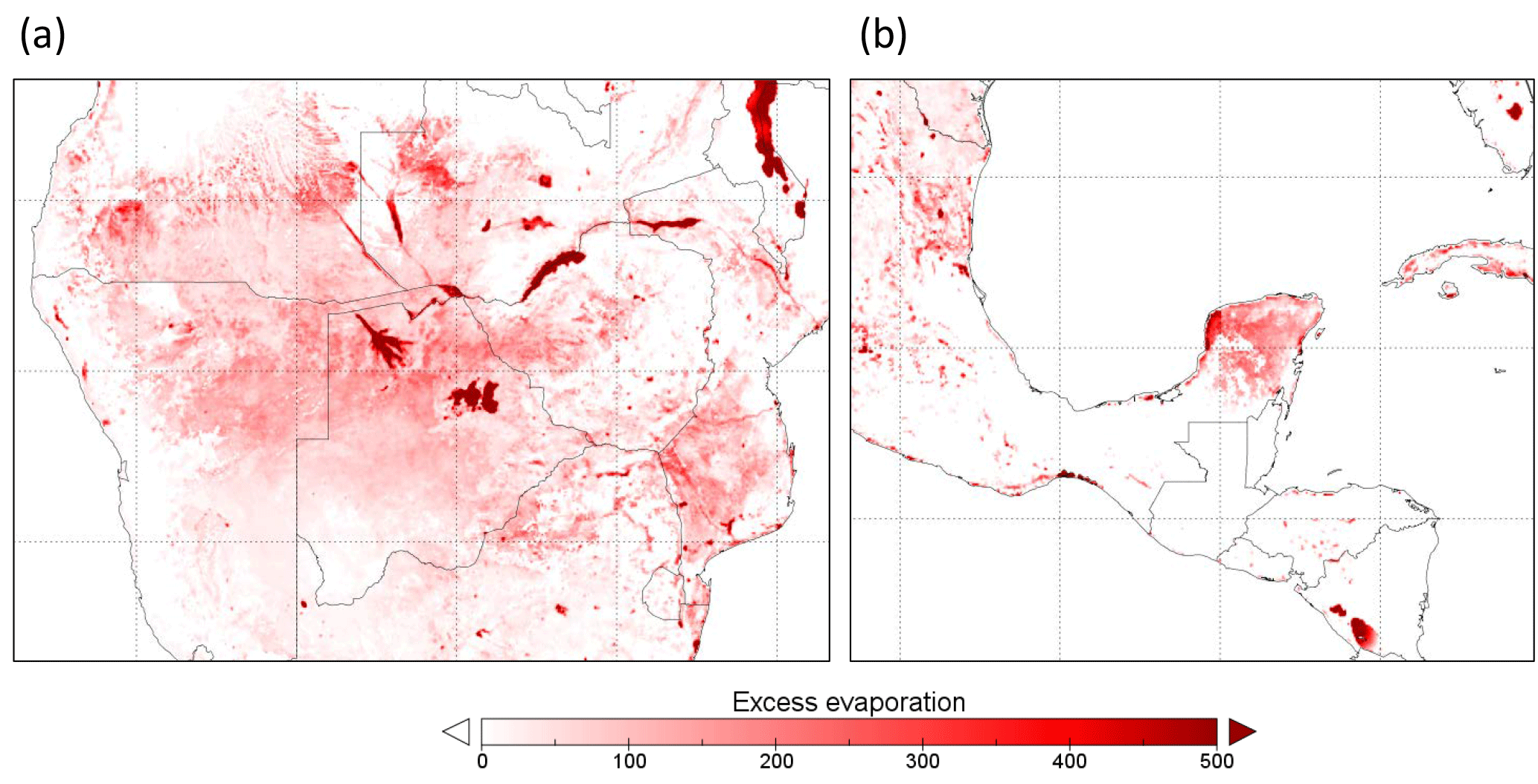
Figure 12 Mean difference between total evaporation and precipitation for 2001–2014 for (a) Botswana, (b) the Yucatán peninsula and surrounding areas.

4.2 Uncertainty in irrigation water requirement estimation

The total estimate of the minimum irrigation water requirement (I₀) at the global scale was about a third lower than previous model-based estimates (Siebert et al., 2010; Wada et al., 2014; Siebert and Döll, 2010). There are some likely explanations for this. Firstly, the diffuse distribution of areas equipped for irrigation (Fig. 3) means that the LST signal from irrigation will likely have been too small to estimate the associated I₀ correctly everywhere. An insufficient LST signal is most likely for grid cells and countries with a temperate, humid climate and highly distributed irrigation, such as the US, where our estimate of I₀ was twice as small as published previously. Conversely, irrigation evaporation estimates should be more accurate in hot, arid regions with large and concentrated irrigation, such as Egypt's Nile delta (Fig. 1). The temporal pattern of the evaporative fraction for this grid cell corresponds well with that of the vegetation cover (Fig. 1e) and reaches values that appear realistic, even more so when considering that only around 80 % of the grid cell was irrigated (Fig. 1a).

Second, previous studies have estimated crop water use (and I₀ from that) using the FAO method of Allen et al. (1998). This method assumes a crop growing well, which is unaffected by ineffective or insufficient irrigation, unfavourable weather, nutrition and soil, pests and diseases or other growth-limiting factors. The resulting crop water use estimates are likely to represent idealized conditions and may be higher than actual water use.

Third, errors in irrigation area mapping are also likely to have played a role. It is noteworthy that the MIRCA2000 mapping used here (Portmann et al., 2010) indicated that 100 % of the grid cell in Fig. 1a was equipped for irrigation. This is not the case, as most unirrigated areas are settlements. Previous studies assumed the entire area was available for irrigation and this difference alone caused their I₀ estimates for this particular grid cell to be 25 % higher. While these numbers relate to a single grid cell, they serve to demonstrate that incorrect mapping of irrigation areas can have a considerable impact on I₀ estimates. In another example, any irrigation outside the grid cells indicated as having at least some irrigable area in the MIRCA2000 mapping would be wholly attributed to non-irrigation forms of secondary evaporation.

Despite these caveats, it is highly likely that true irrigation water application is greater than our estimate I₀, as it was defined as a hypothetical quantity that might occur under conditions of optimally efficient irrigation. Previous studies have made similar assumptions. In reality, field-level irrigation efficiency is reduced by additional drainage below the root zone and any surface runoff that may occur. Further uncertainties are introduced through the necessary assumptions about rooting depth and root zone storage capacity. The comparison with FAO-reported W estimates suggests project efficiencies that are lower than those assumed in previous studies, but the overall correlation between country I₀ and W volumes was high and cannot solely be attributed to differences in irrigated area (Fig. 6). A comparison of country I₀ and W expressed as area-average rates indicates contrasts in project efficiency that are expected in several cases. In other cases, values are outside a plausible range. At least some of these poor estimates are likely related to the aforementioned inaccuracies in irrigation mapping (e.g., Chile and the United Arab Emirates in Fig. 6b).

Overall, the method developed here shows a promising approach for estimating irrigation water use. Estimation at an even higher spatial resolution should help to detect the LST signal more accurately where irrigation areas are dispersed and will thus produce better estimates of E^′. This provides a powerful argument in support of “hyper-resolution” water balance observation and modelling (Wood et al., 2011). All satellite-derived inputs are available at a resolution that is about an order of magnitude finer (500–1000 m) than used here, and computational data assimilation at this resolution is also already feasible. The main impediment is the resolution and quality of irrigation area mapping, which is required to attribute secondary evaporation to irrigation and other sources. The E^′ estimates themselves may assist in mapping, along with information on temporal vegetation patterns and open water mapping and relief, among others. This is an avenue we hope to pursue in future.

4.3 Importance of secondary evaporation in the global water cycle

Our analysis suggests that secondary evaporation makes a meaningful contribution to global evaporation (8.1 %) and reduces the amount of discharge to the oceans by ca. 16 %. At the global scale, irrigation is responsible for only a small fraction of this reduction (ca. 5 %), with the remainder occurring from waterbodies and wetlands. These global averages hide significant regional variation. For example, irrigation plays an important role in the evaporation of river flows in the Nile, Indus and Murray–Darling basins, where most of the discharge is evaporated before reaching the ocean. About half of the total global secondary evaporation is from permanent freshwater bodies, including from some very large waterbodies such as the Caspian sea, the Great Lakes and the African Rift Valley lakes.

There is a strong seasonal cycle in secondary evaporation at the global scale, driven by evaporation from extensive surface waterbodies in formerly glaciated regions in the Northern Hemisphere. This illustrates the profound impact that glaciation has had on regional landscape hydrology and its influence at the global scale.

We estimated global terrestrial evaporation to be 508 mm yr⁻¹ per unit land area or 75.5×10¹² m³ yr⁻¹ total for 2001–2014, made up of 467 mm yr⁻¹ or 69.6×10¹² m³ yr⁻¹ primary evaporation and 41.2 mm yr⁻¹ or 6.1×10¹² m³ yr⁻¹ secondary evaporation. This is close to estimates derived from previous studies. For example, Miralles et al. (2016) reported 13 estimates of terrestrial E derived from a variable combination of satellite observations and modelling, with an average value of 69.2×10¹² m³ yr⁻¹ and coefficient of variation (CV) of ±10 %. Schellekens et al. (2017) reported a mean of 74.5×10¹² m³ yr⁻¹ (CV of ±6 %) for an ensemble of ten state-of-the-art global hydrological models and land surface models. Some of these differences are attributable to the differences in total area and period considered, but the different datasets also include secondary evaporation losses to different degrees. Given that these represent 8 % of total evaporation, such inconsistencies help to explain differences between estimates.

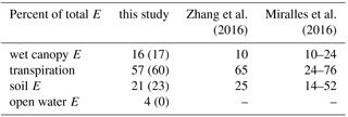
The partitioning between primary evaporation components is within the range of recently published estimates, though it is noted that those ranges are broad (Table 4). Secondary evaporation is fully responsible for open water evaporation and has no impact on wet canopy evaporation; both are a logical consequence of the way these terms are conceptualized. It is estimated that global transpiration and soil evaporation are both enhanced by about 4.5 % due to secondary evaporation of surface and groundwater resources. Irrigation is responsible for a tenth of this increase, with the remainder due to natural processes. Because of the coupling between transpiration and carbon uptake, it can be assumed that these enhancements will increase the global carbon uptake by a similar proportion. Once again, these small contributions apply at global scale, but there are strong differences locally and regionally.

Table 4 Estimated percentage of total (or primary between brackets) terrestrial evaporation (E) contributed by different pathways, compared with estimates from two recent studies.

Thiery et al. (2017) simulated the global impact of irrigation using coupled land surface and atmosphere models. They estimated an evaporation increase from irrigation of 418 km³ yr⁻¹, which was of a similar magnitude to the 300 km³ yr⁻¹ we found. Despite this small contribution to total global evaporation, their modelling did predict small but meaningful reductions in high-temperature extremes over and near large irrigation areas; irrigation rates tend to be highest during hot and dry conditions. To the best of our knowledge, there have been no studies on the impact of wetlands and waterbodies on regional and global climates so far. Given that we estimate these other forms of secondary evaporation to be 20 times greater than that from irrigation, their impact on the atmosphere should be significant.

5 Conclusions

We presented a methodology to assimilate thermal satellite observations into the global hydrological model W3 at a resolution of 0.05^∘ to estimate the secondary evaporation of surface and groundwater resources. In addition, we used a simple irrigation water balance model to estimate the minimum irrigation requirement (I₀) globally. Our main conclusions are as follows:

1. The method developed produces realistic temporal and spatial patterns in secondary evaporation. Accounting for secondary evaporation measurably improved water balance estimates for large closed and open basins, reducing bias in the overall water balance closure from +38 to +2 mm yr⁻¹.

2. Our I₀ estimates were lower than country-level estimates of irrigation water use produced by other model estimation methods for three reasons. Firstly, at the 0.05^∘ resolution, much of global irrigated land occupies only a small part of individual grid cells and may not reduce LST sufficiently to be accurately estimated. Second, our I₀ estimates reflect actual evaporation, which can be lower than idealized crop water use estimates used in previous studies. Third, spatial errors in irrigation area mapping directly affect the attribution of secondary evaporation to irrigation. Overall, actual irrigation application will most likely be higher than estimated here but possibly lower than reported previously.

3. The role of irrigation water use in secondary evaporation is minor at the global scale, accounting for 5 % of total secondary evaporation and 0.4 % of total terrestrial evaporation. Nonetheless, water withdrawals and irrigation evaporation are an important part of the water balance in some regions.

4. Around 16 % of globally generated water resources evaporate before reaching the oceans or from closed basins, enhancing total terrestrial evaporation by 8.8 %. Of this secondary evaporation, 5 % is evaporated from irrigation areas, 58 % from waterbodies and 37 % from other surfaces.

5. Lateral inflows of surface and water resources were estimated to increase global plant transpiration by ca. 4.5 %. The impact on global carbon uptake would be expected to be of similar magnitude. Previous studies have predicted that irrigation evaporation affects regional and global climate. Given evaporation from wetlands and permanent waterbodies is an order of magnitude larger, their impact on the climate system should be pronounced.

There is scope for further improvement in accounting for natural and anthropogenic secondary losses by applying the model-data assimilation approach developed here at higher resolution. This is conceptually straightforward and computationally achievable. Key developments required include more accurate and detailed dynamic observational data on surface water dynamics and more accurate mapping of areas equipped for irrigation.